INTRODUCTION
Understanding floristic patterns and explaining processes that control the distribution of species is an important issue for both scientific and practical goals, particularly in tropical forests. Among the different mechanisms considered to explain rain-forest diversity, soil filtering is often highlighted. In Amazonia, the influence of soil properties on tree communities is frequently addressed at local scale through studies that focus on extreme soil conditions, such as white sands or varzea (Fine et al. Reference FINE, GARCIA-VILLACORTA, PITMAN, MESONES and KEMBEL2010, Fortunel et al. Reference FORTUNEL, PAINE, FINE, KRAFT and BARALOTO2014, Wittmann et al. Reference WITTMANN, HOUSEHOLDER, PIEDADE, DE ASSIS, SCHÖNGART, PAROLIN and JUNK2013). More subtle influences due to moderate variation in soil drainage or chemical composition have also been demonstrated in terra firme forests (Haugaasen & Peres Reference HAUGAASEN and PERES2006, Pélissier et al. Reference PÉLISSIER, DRAY and SABATIER2002, Sabatier et al. Reference SABATIER, GRIMALDI, PREVOST, GUILLAUME, GODRON, DOSSO and CURMI1997, ter Steege et al. Reference TER STEEGE, JETTEN, POLAK and WERGER1993).
However, the relative importance of soil filtering on overall rain-forest diversity is very difficult to estimate due to the scarcity of large-scale data on soil properties (Higgins et al. Reference HIGGINS, RUOKOLAINEN, TUOMISTO, LLERENA, CARDENAS, PHILLIPS, VASQUEZ and RÄSÄNEN2011, Phillips et al. Reference PHILLIPS, VARGAS, MONTEAGUDO, CRUZ, ZANS, SANCHEZ, YLI-HALLA and ROSE2003, Sollins Reference SOLLINS1998). In fact, the soil filtering effect has rarely been directly tested at large scale but is usually approximated from old and inaccurate maps, coarse soil maps (Réjou-Méchain et al. Reference RÉJOU-MÉCHAIN, FAYOLLE, NASI, GOURLET-FLEURY, DOUCET, GALLY, HUBERT, PASQUIER and BILLAND2011) or through indirect co-variables such as geological substrate (Fayolle et al. Reference FAYOLLE, ENGELBRECHT, FREYCON, MORTIER, SWAINE, REJOU-MECHAIN, DOUCET, FAUVET, CORNU and GOURLET-FLEURY2012) and topographic position (Couteron et al. Reference COUTERON, PÉLISSIER, MAPAGA, MOLINO and TEILLIER2003). Geomorphology has also been proposed as an efficient proxy for predicting soil properties (Sombroek Reference SOMBROEK2000) because it incorporates the combined effects of geology, climate and erosion on soil development. As a matter of fact, the influence of geomorphological features on rain-forest diversity has often been reported in different Amazonian regions (Figueiredo et al. Reference FIGUEIREDO, COSTA, NELSON and PIMENTEL2014, Higgins et al. Reference HIGGINS, RUOKOLAINEN, TUOMISTO, LLERENA, CARDENAS, PHILLIPS, VASQUEZ and RÄSÄNEN2011, Phillips et al. Reference PHILLIPS, VARGAS, MONTEAGUDO, CRUZ, ZANS, SANCHEZ, YLI-HALLA and ROSE2003) and linked to variation in soil properties or in the chemical composition of the parent material. However, geomorphological features also represent the varying sensitivity of regions to ancient surface processes and global changes (Thomas Reference THOMAS2012) that have driven morphogenesis. They can then be assumed to reflect Quaternary history or more ancient biogeographical events that may have directly influenced species dispersal and ecosystem functioning. In this view, the influence of geomorphology on rain-forest composition would be mainly linked to divergence in forest dynamics (Hammond Reference HAMMOND and Hammond2005) and species migration.
In a previous paper, we demonstrated the significant influence of geomorphology on floristic patterns at regional and landscape scales in French Guiana (Guitet et al. Reference GUITET, PÉLISSIER, BRUNAUX, JAOUEN and SABATIER2015) using large forest inventories and a precise geomorphological map, but we did not assess to what extent this influence may be driven by soil filtering. In this study, we used the same large dataset (3132 plots, 0.2-ha in size) combined with 421 soil cores to assess the relationships between geomorphological features, soil properties and forest composition in French Guiana. Using variance partitioning to quantify and factor out the environmental effects on the rain forest composition, we tested the hypothesis that current edaphic filtering is not enough in itself to explain the influence of geomorphology on floristic composition and that a significant share of floristic variation accounted for by geomorphic features is caused by other processes such as species migration history and long-term dynamics.
METHODS
Study area
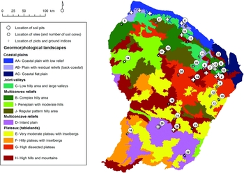
French Guiana occupies 85000 km² in the eastern part of the Guiana Shield, north of Brazil. The climate is equatorial with a short dry season (< 3 mo) and rainfall ranging from 2000 to 4000 mm y−1. The territory is usually described as a smooth plateau inclined from south to north with a mean altitude of 140 m asl. In fact, it exhibits various geomorphological landscapes (Guitet et al. Reference GUITET, CORNU, BRUNAUX, BETBEDER, CAROZZA and RICHARD-HANSEN2013): plains (A) on the coast extended by valley networks in the interior (C); multi-convex reliefs dominated by more or less regular hills in north-west (B, I, J); more or less dissected plateaux in the south-east (E, F, G) interrupted by multi-concave reliefs (D) and by isolated ‘mountains’ (H) that rarely exceed 800 m (Figure 1). It developed on an old Precambrian plutonic and volcanic basement (2.2–1.9 Gy) with a northern coastal belt of sedimentary rocks (Quaternary deposits in the coastal lowlands, rare Precambrian sandstones, conglomerates and quartzite formations). Intact and managed rain forests cover more than 90% of the territory.
Locations of the 33 study sites, with soil samples and forest inventories, and of the 24 soil pits in French Guiana. The colours on the base map indicate the different geomorphological units described in Guitet et al. (Reference GUITET, CORNU, BRUNAUX, BETBEDER, CAROZZA and RICHARD-HANSEN2013). The studied sites are indicated by white circles and the number of soil cores by sites is given in the circles. Locations of plot surveys are indicated by little diamonds. Locations where pits were dug are indicated by white crosses.

Floristic data
The data we used to characterize floristic composition came from forest inventories conducted by ONF (French National Forest Agency) between 2006 and 2013 (Figure 1). These data were presented and analysed in a previous paper (Guitet et al. Reference GUITET, PÉLISSIER, BRUNAUX, JAOUEN and SABATIER2015) that highlighted the influence of geomorphological landscapes on floristic patterns. All palm trees and trees with a stem diameter at breast height (dbh, i.e. at 1.3 m from the ground or above the buttresses if any) > 20 cm were inventoried on 3132 plots, 0.2 ha in size (20 × 100 m) along 111 2.5- to 3-km-long transects at 33 different sites distributed throughout French Guiana (Figure 1). The total dataset included 123906 trees belonging to 51 families and 221 taxa (species or group of species corresponding to a vernacular name). Twenty-nine per cent of the individuals could be identified to species, 64% only to genus and 6% only to family (Guitet et al. Reference GUITET, PÉLISSIER, BRUNAUX, JAOUEN and SABATIER2015). The taxonomic consistency of these forest inventory data was cross-checked using botanical data and double-blind determination. These data proved 83% accuracy at the family level and 74% accuracy at the most precise taxa level. They provided correct estimates of Gini–Simpson beta-diversity at both local and regional scales (Guitet et al. Reference GUITET, SABATIER, BRUNAUX, HERAULT, AUBRY-KIENTZ, MOLINO and BARALOTO2014).
Soil dataset
Three types of soil data were collected over the region (Figure 1): (1) 3132 ground indicators systematically documented in the inventory plots and used to identify locally extreme soil conditions, such as swamps; (2) 421 soil cores (with a 7-cm-diameter hand-auger to a depth of 1.2 m) located along the 111 transects and used to identify soil types on terra firme; (3) 24 soil pits (1.5 m in depth) located away from our transects at representative points with respect to the dominant geology, climate and topography, which provided local reference soil characteristics.
Ground ecological indicators
The 3132 plots were georeferenced using GPS (Garmin 76CSx). For each plot, we recorded the presence of ecological indicators of waterlogged soils (Couteron et al. Reference COUTERON, PÉLISSIER, MAPAGA, MOLINO and TEILLIER2003), such as the presence of typical species as Euterpe oleracea (Arecaceae) and Rapatea paludosa (Rapateaceae), pneumatophores (i.e. respiratory roots) and peat; or very shallow soils indicated by granitic outcrops and superficial duricrust covered by typical low-canopy forest (<15 m) with very abundant lianas (Paget Reference PAGET1999). This survey yielded 188 plots on waterlogged soils assumed to be entirely covered by Gleysols (and rare Histosols), 39 plots mainly situated on shallow soils and assumed to be covered by Petric/Petroplinthic Plinthosol (and rare Leptosols), and 2905 plots on deep well-drained terra firme soils, including some heterogeneous plots (i.e. 307 plots partly on shallow or waterlogged soils).
Soil cores
We sampled 421 soil cores along the 111 transects. The locations were selected in the field as being representative of the variability of topographic positions and of the geological substrate at each site. All the soil cores were georeferenced using GPS and assumed to represent the 0.2-ha plots where they were located. For each soil core, seven layers were described in the field (0–10 cm, 10–20 cm and every 20 cm up to 1.20 m) using a standardized protocol documenting soil moisture, colour, texture (by touch), quantity of roots, the nature and quantity of coarse elements, redox features and concretions. We also assessed soil drainage capacity in the field using a standard protocol adapted to local soil features (Boulet Reference BOULET and GERDAT1983, Sabatier et al. Reference SABATIER, GRIMALDI, PREVOST, GUILLAUME, GODRON, DOSSO and CURMI1997), which enabled us to classify soils with deep vertical drainage >1.2 m (DVD), slow drainage due to red alloterite at a depth <1.2 m (Alt), superficial lateral drainage (DLS) or blocked drainage with temporary hydromorphy (UhS for ‘uphill systems’ and DhS for ‘downhill systems’ depending on their topographic position) and soils with superficial permanent hydromorphy (HS). Samples were systematically collected in each soil core at 20-cm intervals from the surface to a depth of 120 cm and dried as soon as possible for laboratory analyses.
Soil pits and laboratory analyses
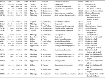
Soil pits had previously been dug in the framework of a permanent plot network and were located at representative points with respect to the geological substrate, topographic position and local climate. We selected 18 pits at 11 sites to represent the variability of soil types. We completed the dataset by digging six additional soil pits at three new sites (Table 1). Pit depths ranged from 105 to 180 cm, average 150 cm, for 1.5 × 1-m pits. We described soil pits using a standard national protocol (Baize & Jabiol Reference BAIZE and JABIOL1995).
Characteristics of soil pits used as reference for soil types in French Guiana including location (coordinates in WGS 84 UTM 22N), depth (cm) of the profile, classification in the World Reference Base (WRB – version 2014) and characteristics of their environment regarding topographical position on the field, geomorphological landscape, geological substrate and approximate annual rainfall (mm y−1).

All the soil samples were analysed at the CIRAD laboratory in Montpellier, France. Analyses were conducted on all soil pit profiles and on a representative sub-sample of soil core profiles. We analysed the percentage of five classes of particle size (clay, fine silt, coarse silt, fine sand, coarse sand), the relative volume of coarse fragments, and carbon and nitrogen content in all the samples. We also analysed pH (water), total phosphorus, available phosphorus (Bray2), CEC and exchangeable bases (using the Metson method at pH 7) in all the soil pit profiles but only in the uppermost soil core horizon (i.e. 0–20 cm). We completed the analyses with Fe/Al/Si extraction by CBD, oxalate and pyrophosphate, total elements (Si, Ca, Mg, K, Na, Fe, Al, Ti, Mn), pH (KCl1N) in all the soil pit profiles. We then computed several soil property indices used in the WRB key: C/N, ∆pH (pH KCl – pH water), ΣB (Caexch + Mgexch + Naexch + Kexch), ECEC (S+Alexch), CEC and ECEC for clay, Feox/FeCBD, ΣRB (CaO + MgO + Na2O + K2O). We also computed the redness rating (RR; Torrent et al. Reference TORRENT, SCHWERTMANN, FECHTER and ALFEREZ1983) and added the water dispersible clay determination when it was useful to distinguish ferralic and argic horizons. All data are available from the authors on request.
Statistical analyses
Soil classification
We used the most recent version of World Reference Base (WRB) to classify our soil profiles (IUSS 2014). Soil pits were classified based on the properties of the diagnostic horizons detected with laboratory analyses and/or morphological criteria observed in the field. We indicated the reference soil group (RSG) of each soil, and associated qualifiers that made it possible to distinguish major variations in the characteristics of the main RSG classes (see Quesada et al. Reference QUESADA, LLOYD, ANDERSON, FYLLAS, SCHWARZ and CZIMCZIK2011, who detailed the most useful qualifiers for Amazonian soils).
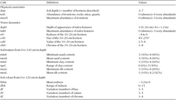
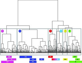
As diagnostic horizons could not be directly assessed to classify the soil cores with the field description, we used an indirect approach based on multivariate analyses. We computed 20 synthetic ordinal indices on physical constraints, water drainage, chemical composition and variation in particle size distribution (Appendix 1). Physical constraints were described by the soil depth and the abundance of very coarse fragments (mainly parental material and ironstone). Water drainage and chemical composition were described using the abundance of redox features but also variation in soil colour that indicate waterlogging (Blavet et al. Reference BLAVET, MATHE and LEPRUN2000), organic matter content (Wills et al. Reference WILLS, BURRAS and SANDOR2007) and haematite content (Torrent et al. Reference TORRENT, SCHWERTMANN, FECHTER and ALFEREZ1983). Particle size distribution was described on the basis of texture that we assessed by touch and calibrated according to laboratory analyses using specimens. We normalized these 20 variables and applied a principal component analysis (PCA) to summarize the information that structured the data in a few synthetic axes. We then used the scores obtained for the 421 soil cores on the PCA axes with eigenvalues >1 (following the Kaiser–Guttman criterion in order to keep the most possible significant variance, Borcard et al. Reference BORCARD, GILLET, LEGENDRE, Borcard, Gillet and Legendre2011) to categorize the cores using hierarchical classification (HC) with the Ward algorithm. HC made it possible to aggregate the soil samples according to their similarity and provided a complete classification tree that we cut in order to obtain the same number of clusters as the number of soil classes identified in the soil-pit dataset.
To classify these clusters with respect to WRB types, we used laboratory analyses of composite samples obtained by mixing two to five samples taken at the same depth, the same site and the same cluster among the soil-core samples in order to get sufficient material for laboratory analyses. We made at least three composites for the main classes to check for homogeneity of intra-class properties and we compared the classes using non-parametric Kruskal–Wallis tests and multiple HSD-Tukey tests for pairwise comparisons (Hollander & Wolfe Reference HOLLANDER, WOLFE, Hollander, Wolfe and Chicken1973).
Partitioning the influence of soil and geomorphology on forest composition
To assess the influence of soil properties on floristic composition and to compare the effects of soil types and geomorphological landscapes on beta-diversity, we used the same analytical framework as in Guitet et al. (Reference GUITET, PÉLISSIER, BRUNAUX, JAOUEN and SABATIER2015), based on a unified variance decomposition strategy (Pélissier & Couteron Reference PÉLISSIER and COUTERON2007). We used non-symmetric correspondence analysis (NSCA), i.e. specific versions of the broader concept of redundancy analysis (RDA), to partition between-plot species diversity (or beta-diversity) along ordination axes using a metric directly related to Simpson diversity (Pélissier et al. Reference PÉLISSIER, COUTERON, DRAY and SABATIER2003). NSCA emphasizes the most common species, thereby revealing variation in the main floristic background of species assemblages along the most prominent ordination axes. We then performed canonical and partial canonical analyses (Legendre & Legendre Reference LEGENDRE and LEGENDRE1998) to quantify the proportion of diversity (sensu Simpson) explained, or not, by external variables. Referring to the Simpson metric above, these analyses are known as NSCAIV (IV being ‘on Instrumental Variables’) for the canonical analyses, and pNSCAIV for the partial analyses (Couteron et al. Reference COUTERON, PÉLISSIER, MAPAGA, MOLINO and TEILLIER2003). The ratio between the sum of the eigenvalues (i.e. variance) of the floristic tables obtained by NSCAIV with respect to soil factors as instrumental variables, and that obtained by the general NSCA, gives the proportion of diversity explained by the soil effect. Combining pNSCAIV with soil factors as instrumental variables and NSCAIV with geomorphological landscapes gave us the proportion of diversity not explained by the soil effect but by geomorphology.
We also used ANOVA-like pseudo-F ratios and restricted randomization procedures to test the effect of soils and geomorphology on the abundance of each taxon (Couteron & Pélissier Reference COUTERON and PÉLISSIER2004). In order to properly take into account long-distance autocorrelation in large-scale beta-diversity patterns that proved to be partly explained by geomorphology (Guitet et al. Reference GUITET, PÉLISSIER, BRUNAUX, JAOUEN and SABATIER2015), we tested the soil effect in a nested design, i.e. by randomizing the plots' floristic composition between soil types within sites. All analyses were performed using R statistical software version 3.0.
We applied this analytical framework at the family level (family-by-plot table) and at the most precise taxonomic level (taxa-by-plot table). We tested the soil effect by considering the classification of soil types with respect to WRB, and the drainage-capacity classes, independently.
We first applied these analyses only to the plots in which soil cores were collected (deep terra firme soils). Second, we also added plots whose soil properties could be unequivocally inferred from field ecological indicators: waterlogged soils classified as hydromorphic soils (SH) based on drainage capacity and as Gleysol on WRB (even if they may include rare Histosols); shallow soils classified as superficial drainage (DLS) based on drainage capacity and as Petric/Petroplinthic Plinthosols in WRB classes (even if they may include rare Leptosols). However, to get the same sampling effort for all soil types we did not use all the 227 plots corresponding to these very thin or very hydromorphic soils but we introduced a systematic sub-sampling (i.e. 24 plots on wetlands and five plots on shallow soils) in order to respect the relative frequency of these extreme soils in the different landscapes and avoid unbalanced sampling.
RESULTS
Soils classification and properties
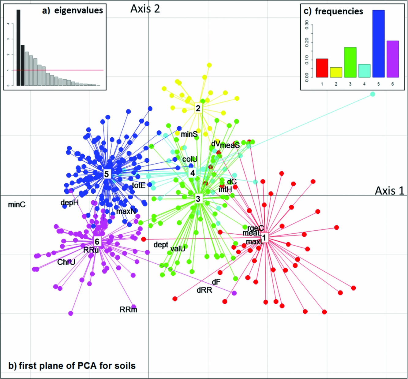
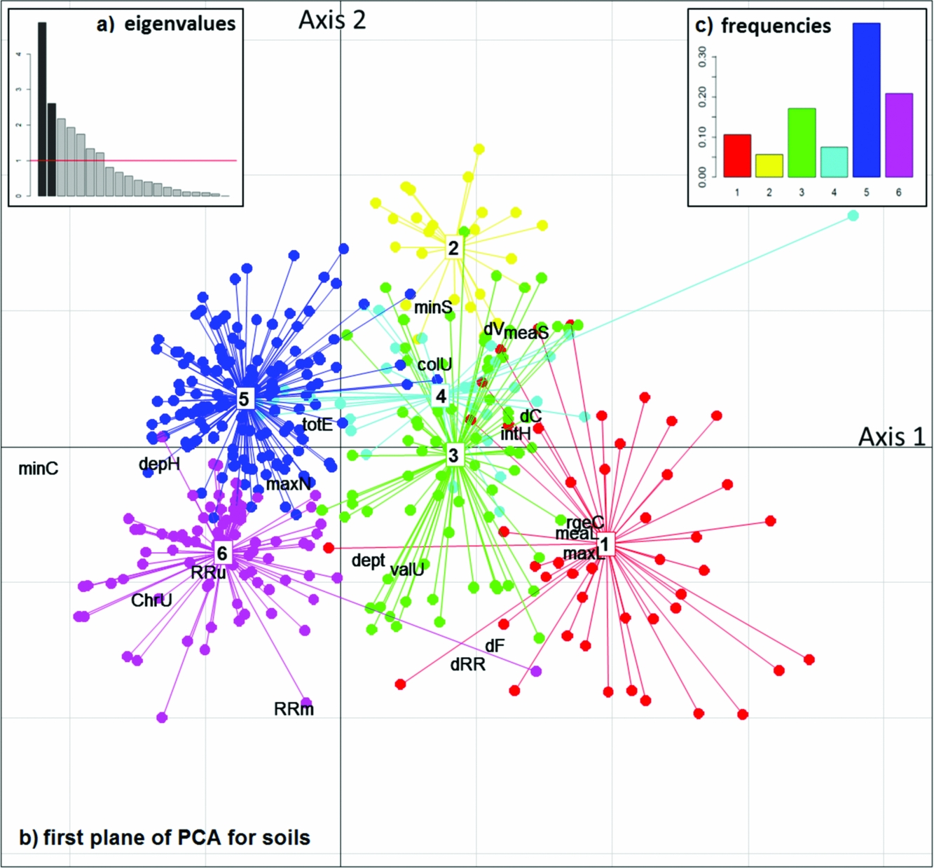
PCA revealed seven notable axes accounting for 80% of total variance (Figure 2). The HC using these seven axes identified six soil types (w1 to w6 – Appendix 2) that were clearly separated on the two first axes of the PCA except for cluster w4, which was better segregated on the third axis (Figure 2). The detailed results of laboratory analyses of the 13 composite samples representing these six clusters are available from the authors on request.
Principal Component Analysis (PCA) based on 20 descriptive variables used for classification of 421 soil cores collected in French Guiana. The two first eigenvalues in dark grey on the histogram (a) total 37% of variance. The projections of the 20 variables on these two main axes (b) are annotated with the codes given in Appendix 1. The points indicate the projections of the soil cores and are coloured according to the six classes defined with hierarchical clustering in Appendix 2. First axis sorts soils with high clay content (minC) and without any signs of hydromorphy (depH) from the most silty or sandy soils (meaL and meaS) showing hydromorphic indices (intH). It opposes on the negative side, Haplic Ferralsols (class 5 in blue) and Geric Ferralsols (class 6 in magenta), that are the most frequent classes as indicated on the barplot (c), to the other types on the positive side. The second axis opposed the soils with the most reddish (RRm) or contrasted colours (dRR, dF) with lots of loam (maxL), classified in the Plinthosols and Cambisols (class 1 in red), to the most sandy (minS) soils with pale upper horizons (colU) especially the rare Arenosols (class 2 in yellow) and Gleyic/Stagnic Acrisols (class 4 in cyan). Acrisols (class 3 in green) have intermediate characteristics.
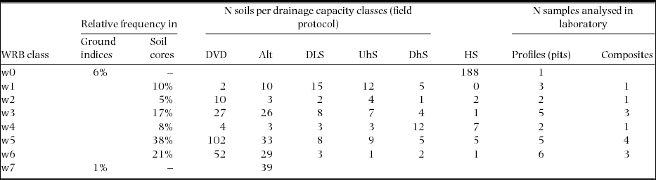
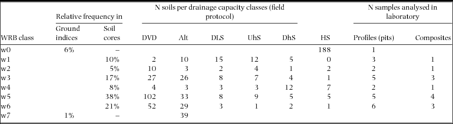
More than half of the soil cores (59%) represented by seven composites were classified in the dominant WRB group of Ferralsols (Table 3, w6 and w5) and associated with 11 profiles among our 24 soil pits. The second group was Acrisols with 25% of soil cores and four composites (w4 and w3) associated with seven profiles. The rest (16% of soil cores for two composites) corresponded to the six other profiles classified in more constraining soil types belonging to Arenosol and Podzol (w2), or Cambisol and Plinthosol (w1).
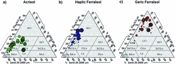
Among the dominant group of Ferralsols, we distinguished two sub-groups: w6 for Geric Ferralsols (Clayic) and w5 for Haplic Ferralsols. The Geric Ferralsols (Clayic) were characterized by a homogeneous high clay content (i.e. >45%) in almost all layers up to 1.20 m deep (Figure 3). The other Ferralsols had a lower clay content with heavy clay texture only in the deepest horizons or very stable clay content from the surface to depth. They contained less than 15% silt in the first 1.20-m layer. By contrast Acrisols had lower clay content (<45%) in all layers, with a marked increase in clay content from the surface to depth (+15–20%) and significant variation in silt content (<30%). Two sub-groups were distinguished among the Acrisols according to redness and the presence of shallow hydromorphic mottles indicating a Gleyic or Stagnic properties: w3 for Haplic Acrisols and w4 for Gleyic or Stagnic Acrisols. Arenosols and Podzols characterized by sandy or sandy loam texture with very low chemical fertility (i.e. CEC < 0.2 cmolc kg−1 and ΣBase < 1.2 cmolc kg−1) were associated with the type w2. Cambisols which had a poorly weathered underlying horizon with high silt content (> 50%) were mixed with Plinthosols characterized by sub-surface Fe-rich layers that contained more than 40% indurated concretions and corresponded to the type w1 marked by very contrasted colours.
Particle size distribution for the three main World Reference Base (WRB) soil groups in French Guiana in the ISSS triangle (International Soil Science Society). Laboratory analyses for soil pit samples are plotted on the triangle with different sizes indicating the depth of the sample in the profiles. For Acrisols (a) clay never exceeds 45% but silt increases with depth: the texture changes from loamy-sand (LoSa) or sandy-clay-loam (SaClLo) in the upper horizons to clay-loam (ClLo), loamy-clay (LCl) or sandy-clay (SaCl) in depth. For Haplic Ferralsols (b) the clay also increases with depth but silt never exceed 20%: texture changes from the sandy-clay (SaCl) in the upper horizons to heavy clay (HCl) in the depth. For Geric Ferralsols (c), the texture is heavy clay (HCl) from surface to depth.

We also compared the drainage capacity of the six soil core classes (gathering UhS, DhS and DLS in one class – Table 2) and observed consistent and significant differences in their distribution within soil groups (χ² = 102, df = 5, P < 0.001). On the one hand, all Ferralsols (w5 and w6) showed good drainage capacity, whereas Gleyic/Stagnic Acrisols (w4) and Cambisols/Plinthosols (w1) had low drainage capacity (Multiple Tukey's test, P < 0.001).
Frequency of the soil types based on World Reference Base (WRB) and drainage classification for our different datasets (soil cores, ground indices and samples for laboratory analysis) in French Guiana: w0 = Gleysol, w1 = Cambisol or Plinthosol, w2 = Arenosol, w3 = Haplic Acrisol, w4 = Stagnic or Gleyic Acrisol, w5 = Haplic Ferralsol, w6 = Geric Ferralsol, w7 = Petroplinthic Plinthosol or Leptosol. DVD = deep vertical drainage >1.2 m, Alt = slow drainage due to red alloterite at a depth <1.2 m, DLS = superficial lateral drainage, UhS = blocked drainage in uphill systems, DhS = blocked drainage in downhill systems, HS = soils with superficial permanent hydromorphy.
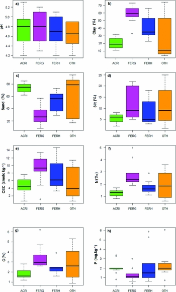
We compared the chemical properties of the three main soil classes, mixing soil pits and composite soil samples (Figure 4, nine samples for Geric Ferralsols, nine for Haplic Ferralsols and 11 for all Acrisols). We focused on carbon, nitrogen, CEC and extractable phosphorus content (method Bray2) in the upper horizon (0–20 cm) that characterize soil fertility. Carbon and nitrogen were significantly more abundant in Ferralsols and especially in Geric Ferralsols than in Acrisols (respectively χ² = 17 and 18, df = 2, P < 0.001 for both). CEC was more variable but still significantly higher in Geric Ferralsols than in Acrisols (χ² = 9, df = 2, P < 0.05). There was no significant difference between soil classes in phosphorus content that was very low in all samples (χ² = 5, df = 2, P = 0.085).
Variability of soil properties in the upper horizon (0–20 cm) between the main soil classes from laboratory analyses of 24 soil pits and 13 soil composites collected in French Guiana. Box-plots indicate the distribution (mean and standard deviation) for the different soil classes (ACRI = Acrisols, FERG = Geric Ferralsols, FERH = other Ferralsols, OTH = other soils) and for the different variables including pH (a), clay content (b), sand content (c), silt content (d), Cation Exchange Capacity (e), nitrogen (f), organic carbon (g) and available phosphorus (h). Whiskers indicate the range and points indicate the extreme values.

Relationship between soils and landscapes
A comparison of the distribution of field ecological indicators for the 3132 plots with Kruskal–Wallis tests revealed significant differences in the frequency of extreme soils between geomorphological landscapes, particularly for Gleysols (χ² = 131, df = 9, P < 0.001). Gleysols were more frequent on plains (18% in type A) and merely infrequent on irregular multiconvex reliefs (3% in type B), moderate plateaux (3% in type E) or mountainous reliefs (4% in type H). Conversely, shallow soils were generally rare (<1%) but more frequent in these three landscape types (χ² = 62, df = 9, P < 0.001) especially on type B irregular multiconvex reliefs (4%) and type H mountainous relief (2%).
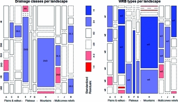
Deep soil types were not equally distributed among landscapes as demonstrated by the distribution of soil types inferred from soil cores (Figure 5, χ² = 181, df = 9, P < 0.001). Plinthosols and Cambisols were particularly abundant in irregular multiconvex landscapes (type B) and in coastal plains (A) but quite rare on high reliefs (H). Arenosols were mainly located in flat areas as coastal plains (A) or multiconcave reliefs (D). Acrisols were also particularly abundant on multiconcave reliefs (D) and regular multiconvex reliefs (I and J). Stagnic and Gleyic acrisols were also frequent on low and regular multiconvex reliefs (I). Conversely, Geric Ferralsols were particularly abundant on all plateaux and high reliefs (type E to H) and Haplic Ferralsols, especially on high reliefs (H) and high plateaux with inselbergs (type F).
Frequency of deep dry soil types per landscape among the 421 soil cores collected in French Guiana. The width of the columns is proportional to the number of samples in the landscape indicated by the letters and described in Figure 1. In each column, height of the rectangles is proportional to soil class frequency in the landscape. Dark shades indicate major deviation from a Chi-square distribution (P < 0.01) and pale shades indicate limited deviation from Chi-square distribution (P < 0.05). Blue indicates positive deviation (frequency higher than expected) and red negative deviation (frequency lower than expected) and white is not significant. Drainage classes (a) vary from deep vertical drainage >1.2 m (DVD) to slow drainage (Alt), superficial lateral drainage (DLS), blocked drainage (UhS for uphill systems and DhS for downhill systems) and soils with superficial permanent hydromorphy (HS). WRB types (b) correspond to Plinthosols or Cambisols (w1), Arenosols (w2), Haplic Acrisols (w3), Gleyic or Stagnic Acrisols (w4), Haplic Ferralsols (w5) and Geric Ferralsols (w6).

Similarly, drainage varied considerably between landscape types (Figure 5, χ² = 24, df = 9, P < 0.005). High reliefs (type H) and moderate plateaux (type E) had the highest proportion of soils with deep vertical drainage. Conversely, low reliefs had the worst drainage: plains and low regular multiconvex reliefs (type I) had significantly less deep drainage and a high frequency of hydromorphic soil (HS) or lateral superficial drainage (DLS); multiconcave reliefs (type D) and joint valleys (type C) had lots of superficial hydromorphy in down-hill positions (DhS); type B (irregular multiconvex landscapes) combined frequent superficial drainage with temporary hydromorphy in uphill positions (UhS).
Effect of landscape and soils on forest composition
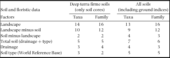
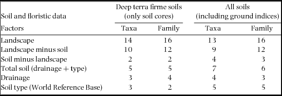
Landscape effects explained from 13% to 16% of the inter-plot variance at the family level and from 10% to 14% at the most precise taxonomic level (Table 3). The proportion of inter-plot variance explained by soil effects ranged from 5% to 6% at the family level and 5% to 7% at the most precise taxon level. The effects of drainage and soil type were highly complementary for deep terra firme soils (only 1% of variance shared), but logically more redundant when we included the extreme soils (2% of variance shared). After factoring out soil effects, landscape effects remained important, about 12% at the family level and from 9% to 10% at the most precise taxon level.
Percentage of Simpson's beta-diversity computed by variance partitioning and explained by soil filtering (effect of drainage and/or soil type) and by geomorphological landscape for different taxonomic levels (family or most precise taxon level) for tree communities in French Guiana.
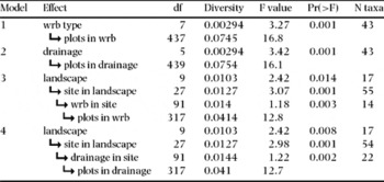
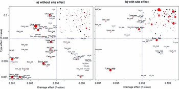
When soil effects were tested alone in the ANOVA-like tests (i.e. models 1 and 2, Table 4), we found 43 taxa whose abundance was significantly explained by drainage (P < 0.05) and 43 influenced by soil types, including 24 shared taxa (Figure 6, Appendix 3).
Results of ANOVA-like test of different models testing soil effects independently (models 1 and 2) or testing landscape, site and soil effects in a nested framework (models 3 and 4) for tree communities in French Guiana. All tests used Simpson metrics. In all cases, total diversity accounted for 0.968 and residual diversity (i.e. intra-plot variance) accounted for 0.89. N taxa indicated the number of taxa with abundances significantly influenced by the tested effect (with P < 0.05). The arrows  indicate that the effects are nested.

Significance of the effects of soils for the 199 species or groups of species (SGS) inventoried in French Guiana and available in the dataset. The 199 SGS are plotted as a function of the P-value of the ANOVA-like tests for drainage and WRB type of soils. Red dots indicate SGS whose abundances are also significantly influenced by landscape. The graph (a) shows the results obtained when effects are tested independently (model 1 and 2). The graph (b) shows the results obtained when the effects of the landscape and soil are tested together and removing site effects (models 3 and 4). Labels indicate the code for SGS listed in Appendix 3.

When landscape effects were tested jointly with soil effects, including sites as permutation compartments to take spatial correlation into account (models 3 and 4, Table 4), all effects remained significant (P < 0.05). The landscape effect was almost the same when tested jointly with drainage or with soil types (df = 9, F = 2.42, P < 0.008). The list of species significantly influenced by landscapes was similar with 17 taxa for both tests including 16 shared taxa (P < 0.05). In these models, drainage significantly accounted for the abundance of only 22 taxa (P < 0.05) and soil type significantly accounted for the abundance of 14 taxa (P < 0.05) (Figure 6, Appendix 3).
DISCUSSION
Soil properties and geomorphological landscapes are highly interdependent
The analysis of our large soil dataset highlighted significant variability of soil properties across French Guiana and confirmed the hypothesis of a strong relationship between geomorphology and soils. Well-drained ferralsols appear to be largely dominant in French Guiana, and represented more than 50% of all our samples, especially in the main geomorphic area corresponding to plateaux, and in the oldest areas corresponding to mountainous landscapes (Figure 5). This situation is consistent with the hypothesis that Ferralsols are widespread on old stable pre-Cambrian basements as generally acknowledged in Amazonia (Quesada et al. Reference QUESADA, LLOYD, ANDERSON, FYLLAS, SCHWARZ and CZIMCZIK2011). However, we observed significant heterogeneity within this group due to variation in clay content (Figure 3). Ferralsols with heavy clay content correspond to the Geric sub-group. They were shown to have higher CEC, C and N contents in the upper horizon than other Ferralsols but slower drainage due to the degradation of the micro-structure (Figures 4, 5). Acrisols were the second most frequent soil type in our samples, like in the rest of Amazonia (Quesada et al. Reference QUESADA, LLOYD, ANDERSON, FYLLAS, SCHWARZ and CZIMCZIK2011). They were mainly concentrated in multiconvex reliefs locally called ‘demi-orange’ that correspond to a geomorphological surface that has undergone significant physical erosion, resulting in a series of small hills (Migon Reference MIGON2009). Acrisols are also frequent in the southern multiconcave reliefs. According to Fritsch et al. (Reference FRITSCH, BOCQUIER, BOULET, DOSSO and HUMBEL1986) in northern Guiana, Acrisols correspond to ancient Ferralsols transformed by erosion (rejuvenation) or eluviation (clay impoverishment), in areas that were subjected to a recent tectonic disequilibrium. They were shown to contain more sand and their upper horizons to contain less carbon and nitrogen than Ferralsols (Figure 4). They also had lower CEC than Geric Ferralsols but contained a little more phosphorus, even if the absolute value was still low. Acrisols are also more poorly drained than Ferralsols with frequent superficial lateral drainage or Gleyic/Stagnic properties (Figure 5). All these characteristics are consistent with observations by Quesada et al. (Reference QUESADA, LLOYD, ANDERSON, FYLLAS, SCHWARZ and CZIMCZIK2011) in the Amazonian basin. More constraining soils, like Gleysols, Cambisols, Plinthosols and Arenosols, were encountered in the coastal plain, and in joint valleys but also in very irregular multiconvex reliefs (Plinthosols on type B) and inland multiconcave reliefs (Arenosols on type D). Gleysols and Plinthosols may result from the transformation of Acrisols related to groundwater oscillations as described by Fritsch et al. (Reference FRITSCH, HERBILLON, DO NASCIMENTO, GRIMALDI and MELFI2007) on the older sediment of the upper Amazon basin. Stagnating water and/or the accumulation of iron concretions in superficial horizons constrains root prospecting in these two types of soil. Arenosols and Cambisols correspond respectively to the oldest and youngest stages of the weathering process undergone by Ferralsols (Quesada et al. Reference QUESADA, LLOYD, ANDERSON, FYLLAS, SCHWARZ and CZIMCZIK2011). Arenosols result from the evolution of Ferralsols after kaolinite weathering. Their coarse soil texture limits their water-holding capacity during the dry season and the nutrients available for the vegetation. Cambisols develop directly on fresh rock exposed by landslides. Their depth and soil structure is generally limited by the presence of shallow saprolites (Ferry et al. Reference FERRY, FREYCON and PAGET2003, Paget Reference PAGET1999). In both cases, available phosphorus is concentrated in the upper horizon and slightly more abundant than in Geric Ferralsols (Figure 4).
In conclusion, the WRB soil classes combined with drainage classes made it possible to describe the variability of the main soil types encountered in the region. The soil variability encountered here is only part of the whole soil diversity described in Amazonia (Quesada et al. Reference QUESADA, LLOYD, ANDERSON, FYLLAS, SCHWARZ and CZIMCZIK2011). Even though the chemical fertility gradient (especially phosphorus, CEC) was rather limited in our study, physical constraints, drainage quality and the nutrient content of the upper horizons were sufficiently contrasted to enable floristic differentiation.
Edaphic filter alone cannot explain the geomorphic control over forest composition
Even if heterogeneous soil distribution confirmed that the different geomorphological landscapes correspond to different assemblages of soil types, our results highlight the fact that the influence of geomorphological landscapes on forest composition involves much more than only a soil filtering effect. It probably also embodies many other relevant processes.
In fact, floristic variance partitioning (i.e. Simpson's beta-diversity) showed that soil filtering has a significant impact on the forest composition at a large scale (Table 4), even if our environmental gradient is quite limited in comparison with the usual studies performed in Amazonia, which focus on highly contrasting habitats, like white sands or varzeas versus terra firme (Haugaasen & Peres Reference HAUGAASEN and PERES2006, Stropp et al. Reference STROPP, VAN DER SLEEN, ASSUNÇAO, DA SILVA and TER STEEGE2011). The soil filtering effects we detected are very consistent with previous results demonstrating the relationship between floristic composition, topography and soil properties at local scale in three experimental sites in French Guiana (Couteron et al. Reference COUTERON, PÉLISSIER, MAPAGA, MOLINO and TEILLIER2003, Morneau Reference MORNEAU2007, Sabatier et al. Reference SABATIER, GRIMALDI, PREVOST, GUILLAUME, GODRON, DOSSO and CURMI1997). The list of taxa influenced by drainage was highly consistent with the list obtained in these studies and included many taxa known to be restricted to hydromorphic soils as well as taxa known to be intolerant to water soil saturation (Appendix 3). Drainage capacity appears to be an influential factor with strong distinction between waterlogged and terra firme soils as demonstrated by Morneau (Reference MORNEAU2007) at Paracou. Drainage capacity also explains the significant change in floristic composition from terra firme soils with deep drainage to terra firme soils with temporary water-saturation as demonstrated by Couteron et al. (Reference COUTERON, PÉLISSIER, MAPAGA, MOLINO and TEILLIER2003) at Counami and Sabatier et al. (Reference SABATIER, GRIMALDI, PREVOST, GUILLAUME, GODRON, DOSSO and CURMI1997) at Piste de St Elie. The species whose abundances are significantly influenced by drainage confirmed some ecological preferences previously reported at these few sites (Appendix 3). However our forest inventory data probably underestimate intra-generic differences. This may prevent our analysis from revealing radiation within large genera such as Eschweilera or Licania for example. The effect of the type of WRB partly overlaps with the effect of drainage because drainage capacity depends on the textural and structural properties of soils that are included in horizon diagnostics. However, it also includes the influence of chemical composition and fertility and is correlated with the abundances of 16 supplementary species that are not concerned by drainage effect.
Finally, the effect of soil filtering partly overlaps with the effect of the geomorphological landscape, in the sense that a large share of this effect vanished when we factored out landscape types (Table 3). Landscape types actually express most of the observed influence of soil types on floristic composition. Yet the converse does not hold since soil types explained only about 25% of total influence of geomorphological landscapes on forest composition at the family level and about 30% at the most precise taxon level. Even if extreme soils inferred from field ecological indicators are relatively rare (<10% of total plots), their influence significantly increased the effect of the soil in the analyses. However, even in this case, the fraction of variance explained by soils is not sufficient to explain the landscape effect. On the contrary, we can conclude that geomorphological landscapes quite efficiently reflect the main variation in regional soil cover as they capture 60% of the soil filtering effects due to soil variation within the deep terra firme soil group. On the other hand, landscape types are not sufficient to represent local extreme conditions as this fraction decreases from 60% to 40–50% when highly constrained soils are taken into account.
Limits of the study and future outlook
Three factors may limit the power of our analysis. First, the small number of available plots (N = 445) and trees (N = 18057) with respect to the number of taxa (N = 199). However, as the proportion of variance explained by geomorphological landscapes is of the same order of magnitude in this sub-sample as in the complete sample (Nplot = 3132) we previously used (Guitet et al. Reference GUITET, PÉLISSIER, BRUNAUX, JAOUEN and SABATIER2015), we can assume that this dataset is sufficient to correctly estimate environmental effects on the floristic composition. However, the actual power of ANOVA-like tests applied species-by-species is probably lower because of the lack of replicates within sites (i.e. a maximum of 29 plots per site). In fact, in this study, the landscape effect significantly accounted for the abundance of only 16 taxa when the site effect was taken into account, whereas it proved capable of explaining the abundance of 80 taxa when tested under the same framework with the complete dataset (Guitet et al. Reference GUITET, PÉLISSIER, BRUNAUX, JAOUEN and SABATIER2015).
Secondly, the taxonomic resolution of our floristic data is often limited to the generic level because of the taxonomic resolution of vernacular names. However phylogenetic niche conservatism (Wiens & Graham Reference WIENS and GRAHAM2005) may reduce the noise due to mixing different species in the same vernacular name. Indeed, recent articles proved that niche conservatism is deeply marked in the phylogeny of tropical evergreen forest trees, and that species from the same family show on average more similar adaptive trends (Hardy et al. Reference HARDY, COUTERON, MUNOZ, RAMESH and PÉLISSIER2012). Moreover, functional and phylogenetic similarities are strongly related in the French Guiana tree communities, such that phylogenetic proximity of species reflects the niche overlap (Baraloto et al. Reference BARALOTO, HARDY, PAINE, DEXTER, CRUAUD, DUNNING, GONZALEZ, MOLINO, SABATIER, SAVOLAINEN and CHAVE2012). As a consequence, groups of species in the same genus, that are gathered under the same vernacular name because of similar trunk/leaf morphology, bark/wood characteristics and timber use, are supposed to be quite homogeneous in terms of niche, even if exceptions due to recent species divergence may exist (Couteron et al. Reference COUTERON, PÉLISSIER, MAPAGA, MOLINO and TEILLIER2003). Moreover our measures of diversity, based on Simpson's metrics and on ratio (i.e. between over total diversity) and used to estimate habitat filtering, are expected not to change with the taxonomic resolution, even in the absence of niche conservatism (Munoz et al. Reference MUNOZ, RAMESH and COUTERON2014). Indeed, when applying our framework on a reduced floristic table using only the reliable taxa at the species resolution (corresponding to 29% of the trees), we verified that habitat filtering measured at the species resolution was equal to the estimate based on the total dataset mainly at the genus resolution (i.e. 7%) and not very different from the result at the family level (i.e. 6% – result not shown). Consequently, the coarse taxonomic resolution of our forest inventory data is not a critical problem and proved to be well-adapted when one measures diversity in Simpson's metrics (Guitet et al. Reference GUITET, SABATIER, BRUNAUX, HERAULT, AUBRY-KIENTZ, MOLINO and BARALOTO2014). We can then assume that the relative proportions of variance explained by the different environmental factors we considered are correctly estimated.
The last limiting factor is linked to the combination of mass effects and local spatial auto-correlation (Phillips et al. Reference PHILLIPS, VARGAS, MONTEAGUDO, CRUZ, ZANS, SANCHEZ, YLI-HALLA and ROSE2003) that may result from the relative homogeneity of the soils at several sites (i.e. the frequency of the dominant class >50% at 14 sites for soil types and at 16 sites for drainage). In fact, where sites are dominated by deep well-drained ferralsols, the edaphic filter on the minority soils may be masked by the important seed sources of dominant species with quite large niche amplitude that used to dominate this type of habitat (Pélissier et al. Reference PÉLISSIER, COUTERON, DRAY and SABATIER2003). This may explain why soil has an impact on the distribution of 62 taxa out of 199 when tested alone, whereas they impacted a more restricted and quite different list of taxa when we controlled for spatial auto-correlation by means of the site effect in the test (Table 4).
Nevertheless, the weak influence of soil filtering that we detected at a large scale is consistent with the results of several previous studies. In fact, niche effect (including soil and climate) rarely explains more than 10–12% of beta-diversity when studied at a large scale (Chust et al. Reference CHUST, CHAVE, CONDIT, AGUILAR, LAO and PEREZ2006, Réjou-Méchain et al. Reference RÉJOU-MÉCHAIN, PÉLISSIER, GOURLET-FLEURY, COUTERON, NASI and THOMPSON2008). This supports the hypothesis that only early-successional stages of forest communities are strongly influenced by niche effects and that mature forests are more neutral (Réjou-Méchain et al. Reference RÉJOU-MÉCHAIN, MULLER-LANDAU, DETTO, THOMAS, LE TOAN, SAATCHI, BARETTO-SILVA, BOURG, BUNYAVEJCHEWIN and BUTT2014). It also supports the hypothesis that soil filtering produces significant floristic variation even if only a minority of taxa displays significant variation in abundance with variation in soil properties (Vleminckx et al. Reference VLEMINCKX, DROUET, AMANI, LISINGO, LEJOLY and HARDY2015).
Finally, the fact that geomorphology explains broad-scale patterns of forest diversity independently of soil filtering effects reinforces the interpretation linking geomorphological landscapes to long-term forest change. In fact, the regional drivers that shaped geomorphological landscapes (local tectonics, global and regional climate changes, marine transgressions) have a direct effect on meta-community dynamics and species dispersion by creating corridors, barriers, fragmentation or refuges (Haffer Reference HAFFER2008) and by modifying forest dynamics (Hammond Reference HAMMOND and Hammond2005, ter Steege et al. Reference TER STEEGE, Hoorn and Wesselingh2010). Consequently, each geomorphological landscape can be viewed as an indicator of a long ecological and biogeographic trajectory, which is specific to the region and that directly and indirectly shaped forest composition via neutral migration limitation effects, niche effects and complex interactions between the two processes over long periods of time (Leibold et al. Reference LEIBOLD, HOLYOAK, MOUQUET, AMARASEKARE, CHASE, HOOPES, HOLT, SHURIN, LAW, TILMAN, LOREAU and GONZALEZ2004). A precise and systematic analysis of geomorphological features may be the best way to advance our understanding of patterns of diversity in tropical forests.
ACKNOWLEDGEMENTS
We wish to thank the French Forest Agency (ONF), the Guianese National Park (PAG), the French Ministry of the Environment's ECOTROP programme (Paysages et Biodiversité), and the European Union's PO-FEDER program (HABITATS) for funding this study. We would also like to thank Fabrice Benedet for organizing the database, and all the colleagues who participated in soil pits opening and description: Mathilde Desprez, Jerome LeFol, Dominique Paget and Bruno Ferry.
APPENDICES
List of the 20 indicators used to classify soil cores in Principal Component Analysis (PCA) and based on descriptions of the soil samples realized on the field in French Guiana during our study. The codes indicated in the first column are those used in Figure 2. Colour indices were computed using Munsell code values and soil texture indices were calibrated using laboratory analyses of 20 specimens used as references.

Classification tree of our 421 soil cores obtained after Principal Component Analysis (PCA) and Hierarchical Clustering (HC). The terminal branches correspond to soil cores and are merged regarding the similarity between samplings. The tree is cut to provide six clusters indicated by the coloured symbols and numbers (i.e. w1 to w6). The coloured boxes indicate the extreme positions of the soil cores that were mixed in the composite samples (designated with letter codes) and used for laboratory analyses to interpret the clusters (available from the authors on request).

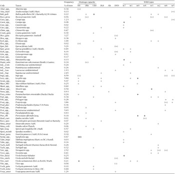
ANOVA-like tests for the effects of soil filtering on the abundance of the 199 tree taxa inventoried in French Guiana. Only taxa with a significant P-value (P < 0.05) for ANOVA-like tests are included. Signs symbolize the results of comparison tests based on Tukey HSD (honest significant difference). + indicates that the abundance is significantly higher in the class than in all other classes; − indicates that the abundance is significantly lower in the class than in all other classes; parentheses indicate that the abundance is significantly higher or lower in the class than some other classes (but not all). Codes for species are those used in Figure 6. Codes for soil types are w0 for Gleysols, w1 for Plinthosols & Cambisols, w2 for Arenosols, w3 for Haplic Acrisols, w4 for Gleyic or Stagnic Acrisols, w5 for Haplic Ferralsols, w6 for Geric Ferralsols and w7 for Leptosols and Petroplinthic Plinthosols. Codes for drainage capacity: DVD for deep vertical drainage >1.2 m, Alt for slow drainage due to red alloterite at a depth <1.2 m, DLS for superficial lateral drainage, UhS for blocked drainage in uphill systems, DhS for blocked drainage in downhill systems, HS for soils with superficial permanent hydromorphy.