


We consider the relationship between the preferences of American voters and those of their elected U.S. legislators, namely, the senators and members of the U.S. House who collectively represent them. We seek to understand what might be termed the federal representation process, a process wherein the preferences of American voters generate a set of federal legislators with their own preferences, which in turn generate aggregate House and Senate preferences. Given that the dominant political parties in the country are polarized, how does this process work? To answer this question, we characterize the extent to which there is congruence between the preferences of voters and the preferences of their corresponding members of Congress. We also characterize the extent to which there is congruence between aggregate American voter preferences and aggregate preferences at the congressional chamber level.
These dual characterizations reflect the fact that one can conceptualize the federal representation process as operating at two levels. At a micro-level, individual voters elect members of Congress, and accordingly, one can inquire whether a given voter is adequately represented by senators and a particular representative. At a macro-level, the collection of senators and representatives specify chamber aggregates such as the Senate median, and in this light, one can consider whether a representative American voter, say, the median American voter, is represented in the two chambers of Congress.
As we show, our analysis of the federal representation process highlights a distinct lack of congruence between federal legislators and their constituencies. We show that this lack of congruence is due to the fact that both senators and House members are politically extreme compared to the voters who put them in office. Our evidence implies that micro-level congruence is not a feature of the contemporary federal representation process and that, in particular, this process has what one might call a leapfrog aspect to it.
To best understand this idea, consider a hypothetical election in a congressional district in conjunction with two alternative scenarios. In the first scenario, voters choose between candidates who closely approximate the district median voter; in this scenario, incumbent House members and those who want to replace them have converged to district medians. In a contrasting second scenario, House members are political extremists, and elections are contests between two poles, one on the political left and one on the right. In the latter scenario, when a right-leaning representative is replaced, his or her replacement is a left-leaning extremist. When this sort of replacement occurs in a congressional district, the district median voter is leapfrogged: left-leaning partisans much prefer the new representative to the old, whereas right-leaning partisans feel the opposite, and moderates remain relatively poorly represented both before and after.
Our evidence suggests that what we are calling leapfrog representation—the first scholar, we believe, to identify a pattern like this in Congress was Fiorina (Reference Fiorina1974)—operates at the congressional district and state levels. Although we cannot say exactly why this is the case, the evidence we bring to bear on our analysis of representation suggests that elected officials tend to represent the preferences of engaged voters more than they do disengaged voters and, furthermore, that engaged voters tend to be relatively extreme. We measure an individual's level of political engagement by his or her donating behavior, and we show that there is more congruence between donators and their representatives in Congress than between nondonators and the elected officials who represent them.
Leapfrog representation causes distortion at the micro-level, and we show that there is a corresponding distortion in representation at the House level. In this analysis, we consider two Congresses, the 109th and the 110th. As we will show, we find that the 109th House was too conservative compared to the median American voter, and the 110th House was too liberal. In short, the median American voter was leapfrogged at the aggregate House level. We do not see evidence of leapfrogging in the Senate, and we suspect that this is attributable to the greater insulation from public opinion afforded this chamber. Indeed, one of the motivating ideals of the Senate was that, as noted in Federalist No. 63, “It may be suggested, that a people spread over an extensive region cannot, like the crowded inhabitants of a small district, be subject to the infection of violent passions, or to the danger of combining in pursuit of unjust measures.” Here, “a people spread of an extensive region” refers to the residents of a state, and “crowded inhabitants of a small district” refers to members of a congressional district. Moreover, in Federalist No. 62, it is written that, “The mutability in the public councils arising from a rapid succession of new members, however qualified they may be, points out, in the strongest manner, the necessity of some stable institution in the government.” In other words, the Senate, due to its longer term length (six years) compared to that of the U.S. House (two years), is intended to be less volatile and more moderate than the House.Footnote 1 Our evidence, drawn from the transition from the 109th Congress to the 110th, is consistent with this intention.Footnote 2
We next discuss various theories of representation, and following that, we explain how we engage our key research questions about representation and the representation process. We then present our statistical model, describe the data we use to fit it, and discuss results. We end with caveats and suggestions about future research.
VOTER REPRESENTATION BY ELECTED OFFICIALS
There are few questions as fundamental to democratic politics as those pertaining to preferences and representation. To the extent that representation is a feature of the U.S. polity at the federal level, it presumably flows from the country's regular elections that staff key institutional positions in Washington, DC. Nonetheless, simply because regular elections occur does not mean that the officials who win these elections represent voters and that Americans writ large are represented in Congress or by the president.Footnote 3
Theoretical Literature on Representation
What one might call the standard argument as to why elected officials should be expected to represent their constituents can be found in Downs (Reference Downs1957), who argues that candidate competition under suitable regularity conditions is sufficient to guarantee that a single-member electoral district is represented by an official who locates at the district's median voter. The literature on candidate competition, median convergence, and so forth is extensive (e.g., Alesina and Rosenthal Reference Alesina and Rosenthal1996; Calvert Reference Calvert1985; Wittman Reference Wittman, Enelow and Hinich1990), and see Gerber and Lewis (Reference Gerber and Lewis2004) for a review.
Beyond theoretical work that is rooted in spatial voting (e.g., Enelow and Hinich Reference Enelow and Hinich1984, Reference Enelow and Hinich1990) and the median voter theorem (Black Reference Black1958), there are other reasons to believe that elected officials should represent their constituents.Footnote 4 Because elected officials are members of electorates themselves and presumably have been socialized under circumstances largely similar to those of their constituents, one might expect them to have views in common with such people (Erikson and Tedin Reference Erikson and Tedin2001). Elected officials may be representative of the public because they believe this to be a job responsibility (Miller and Stokes Reference Miller and Stokes1963).
Other theories, though, highlight the virtues of a looser relationship between voters and their representatives. For example, some elected officials may regard themselves as independent trustees, tasked with forming expertise in policy areas that transcend the abilities of most members of the public. With this expertise, elected officials make what they believe to be the best decisions on behalf of their electorates, regardless of public opinion (Canes-Wrone, Herron, and Shotts Reference Canes-Wrone, Herron and Shotts2001; Jacobs and Shapiro Reference Jacobs and Shapiro2000). There may also be a middle ground wherein the extent of representation depends on the issue or the context in which an elected official finds him- or herself. For example, on a very salient issue over which elected officials do not have private information, representatives may privilege their electorates. On a more obscure issue or on a issue where the expertise of elected officials dominates the information available to constituents, representatives may act like independent trustees (Wahlke et al. Reference Wahlke, Eulau, Buchanan and Ferguson1962). Finally, there may be a dynamic element to the relationship between representatives and constituents (e.g., representatives who have just been elected to a long term in office may be less responsive to their electorates than politicians facing an immediate and tough reelection challenge) (Elling Reference Elling1982).
Possible virtues notwithstanding, there are a variety of reasons to think that the representation process is not as simple as the median voter theorem might suggest. Federalism as implemented in the United States divides governmental authority between national and state governments; it allocates most election-related functions to states; and, consequently, election laws and customs vary widely across congressional districts and states (e.g., Kimball Reference Kimball2003). Moreover, the contemporary campaign finance system in the United States protects incumbents from voter retribution and thus has the potential to weaken the relationship between elected officials and their constituents (Miller Reference Miller1999; Zimmerman and Rule Reference Zimmerman and Rule1998). Variance in the extent to which voters are informed about government policy choices can induce nonmedian convergence (Baron Reference Baron1994), and, finally, the fact that access to the ballot box is not universal (Keyssar Reference Keyssar2000) and that certain types of voters tend to have unusually high invalid vote rates (Herron and Sekhon Reference Herron and Sekhon2005; Tomz and van Houweling Reference Tomz and van Houweling2003) militate against a simple representation process in which district median voters are guaranteed to be represented by legislators in Congress.
Empirical Evidence on Representation
Miller and Stokes (Reference Miller and Stokes1963) were among the first to measure quantitatively the extent of congruence between U.S. representatives and members of their districts. In particular, they compared constituency opinions garnered from survey instruments with legislators' (as well as their opponents') opinions and also measured the correlations between constituency opinions and legislators' roll call votes. Miller and Stokes uncovered evidence of representation more strongly on some issues (e.g., civil rights) than on others (e.g., foreign policy, social welfare) and found that election winners were more representative than election losers on matters of social welfare. Miller and Stokes received substantial methodological criticism on the grounds that the degree of actual correspondence between legislators and constituents cannot be correctly measured by a simple correlation coefficient (Achen Reference Achen1977; Erikson Reference Erikson1978).
Achen (Reference Achen1978) revisited Miller and Stokes' (Reference Miller and Stokes1963) analysis and investigated the extent of representation across three theoretically informed empirical measures of association: proximity (the distance between representatives and constituents), centrism (how well a representative minimizes this distance holding constant constituency opinion), and responsiveness (how well a constituency's ideological leanings predict a representative's views). Achen (Reference Achen1978) argued that civil rights opinions were not more accurately represented than other issue dimensions and that winners were not more representative than losers in congressional elections. In another critique of Miller and Stokes, Erikson (Reference Erikson1978) found that, once sampling error is taken into account, the extent of representation is much greater than originally claimed.
In contrast to the aforementioned individual-level focus on representation, in which voters and representatives are compared, some scholars look to aggregate data including, opinion poll results to understand whether government policy outcomes can be attributed to public preferences. There is evidence that a strong correspondence exists in this way (Erikson, MacKuen, and Stimson Reference Erikson, MacKuen and Stimson2002; Stimson, MacKuen, and Erikson Reference Stimson, MacKuen and Erikson1995), although it may be changing over time (Ansolabehere, Snyder, and Stewart Reference Ansolabehere, Snyder and Stewart2001; Jacobs and Shapiro Reference Jacobs and Shapiro1997; Monroe Reference Monroe1998). Evidence also points to a balancing effect whereby too much pressure by elected officials in one ideological direction will move public sentiment in the opposite direction (Erikson, Mackuen, and Stimson Reference Erikson, MacKuen and Stimson2002; Stimson Reference Stimson2004; Wlezien Reference Wlezien1995, Reference Wlezien1996).
Within studies of representation, there is movement toward comparing voters' preferences with legislator roll call voting behavior (i.e., with legislator ideal points). For example, Ansolabehere, Snyder, and Stewart (Reference Ansolabehere, Snyder and Stewart2001) scale the roll call votes of elected representatives and compare resulting ideal point estimates to district presidential vote shares; they find evidence of representation, but it is uneven and varies depending on district and election characteristics over time. Clinton (Reference Clinton2006) examines the relationship between legislator roll call voting behavior and congressional district–level measures of voter ideology; he also highlights the unevenness in legislator responsiveness to constituency preferences. Ansolabehere, Snyder, and Stewart (Reference Ansolabehere, Snyder and Stewart2001) and Clinton (Reference Clinton2006) use methodologies close to ours, as does Jessee (Reference Jessee2009) in his study of representation, which we discuss in detail later.
Representation and Ideal Points
If we conceptualize legislators as having ideal points that drive their roll call voting choices, then we should think similarly about voters. The advantage of thinking about underlying preferences in terms of ideal points is that, under suitable conditions, ideal points can be compared in a proximate sense. That is, we can ask if two ideal points are “close to” one another and thus can inquire about distances between legislators and voters rather than focusing on correlations. If we are interested in studying how well a senator represents his or her state, say, we need to be able to describe measures of proximity between the hypothetical senator and the voters whom he or she represents in Congress.
Ideal points, drawn from the spatial theory of voting, are best thought of as reflecting preferred policy choices in a given policy space. Assuming that the American policy space is unidimensional and aligned left to right, then each voter and elected official can be thought of as having a unidimensional ideal point such that individuals with politically left views have ideal points smaller in a numerical sense than those with politically right views. A given individual's ideal point describes how left or right the individual believes government policy should be.
Individual ideal points, whether they are from legislators or voters, are latent insofar as they inform individuals' choices, but themselves are not directly observable. Empirically speaking, scholars use observed political choices (e.g., does a given individual support or not support abortion rights?) to estimate numeric ideal points on the real line. The statistical techniques used to do this borrow heavily from psychometrics. Psychometricians commonly employ what are called item response models to evaluate the test-taking capabilities of individuals who have answered numerous questions (called items) on a test. Relatedly, political researchers use observed political choices (parallel to test questions) to estimate the left–right locations of legislators or voters.
Ideal point estimates can only be measured or scaled in a relative fashion. For a psychometrician who uses an item response model to estimate intelligence rankings based on the outcomes of test questions, resulting estimates of test-taking abilities show how well a given student performs relative to his or her peers. For political researchers, estimates of left–right ideal points based on observed political choices show how much to the left or the right an individual is relative to other individuals.
Poole and Rosenthal (Reference Poole and Rosenthal1997) revolutionized congressional research by using item response models to estimate the relative ideological leanings of members of Congress using roll call voting choices, and work in this vein has yielded what are called NOMINATE scores. Relatedly, Ansolabehere, Snyder, and Stewart (Reference Ansolabehere, Snyder and Stewart2001) scale ideal points for members of Congress using a technique devised by Heckman and Snyder (Reference Heckman and Snyder1997), along with an adjustment recommended by Groseclose, Levitt, and Snyder (Reference Groseclose, Levitt and Snyder1999) to allow for intertemporal comparability; Londregan (Reference Londregan2000) builds an agenda model into an ideal point estimation framework; and, in recent years, substantial developments have been made in the estimation of ideal points that use Bayesian statistical methods to recast parameter estimation problems into missing data problems (Bafumi et al. Reference Bafumi, Gelman, Park and Kaplan2005; Clinton, Jackman, and Rivers Reference Clinton, Jackman and Rivers2004; Jackman Reference Jackman2001; Martin and Quinn Reference Martin and Quinn2002). Bayesian approaches to ideal point problems have been applied in many different contexts (e.g., Bailey Reference Bailey2007; Clinton, Jackman, and Rivers Reference Clinton, Jackman and Rivers2004; Epstein et al. Reference Epstein, Herron, O'Halloran and Park2007; Martin and Quinn Reference Martin and Quinn2002, Reference Martin and Quinn2007).Footnote 5
A key limitation of ideal point estimation results from the fact that, as noted previously, ideal points are only defined relatively. If, say, one has a set of ideal point estimates for members of the Senate and a set for members of the U.S. House, then these two sets of ideal points will not in general be comparable. When two sets of ideal points are not comparable, it is said that they do not reside in a common policy space. To address our question about representation under polarized parties, both in its micro and macro forms, we need ideal point estimates for both elected officials and voters, and, importantly, we need these ideal points to reside in a common policy space. We now describe the data that we use to scale or locate in a common policy space the president, senators, representatives, and a nationally representative collection of voters.
DATA REQUIREMENTS FOR IDEAL POINT ESTIMATION
Ideal point estimation typically draws on responses to individual-level, binary questions. A binary question is one that has two possible outcomes, often but not necessarily “yes” and “no.” Roll call votes fit this paradigm—if voting, a legislator can either vote in favor of a bill or against it—and survey questions can be binary as well if phrased in an appropriate way. Thus, to estimate legislator, presidential, and voter ideal points in a comparable way, we draw on three linked data sets, each of which contributes binary choices for different groups of individuals.Footnote 6
Binary Choices for Members of Congress
For members of the House and Senate, our set of binary choices consists of all recorded roll call votes cast during the 109th (2005–06) and 110th Congresses (2007–08).Footnote 7 Such roll call votes form the basis of the well-known NOMINATE scores for members of Congress.
Some congressional roll call votes are procedural (e.g., cloture votes in the Senate), and others are up-or-down votes on pieces of legislation. Furthermore, some recoded Congressional votes are on conference committee reports that, by construction, are voted on in both the House and the Senate. Because a conference committee vote is identical in both the House and the Senate, such votes allow us to link the ideal point estimates of senators and representatives. Intuitively speaking, a conference vote is like a test question that appears on two tests, one taken by members of the Senate and one by members of the House. The existence of conference votes allows us to scale senators and House members relative to one another. Beyond conference votes, we treat all other congressional roll calls as being unique to a given chamber.
There were 1,210 recorded roll call votes in the 109th House, 645 in the 109th Senate, 1,865 in the 110th House, and 657 in the 110th Senate.Footnote 8 These numbers include every recorded vote taken in the 109th and 110th Congresses, independently of whether the vote sheds light on underlying legislator preferences. We treat 14 conference votes from the 109th House and 109th Senate as identical in both chambers, and similarly we treat 12 conference votes from the 110th Congress in this way.Footnote 9 After combining conference votes across chambers, there are 1,819 roll call votes from the 109th Congress and 2,510 from the 110th.
There were four legislators from the 109th House who became members of the 110th Senate. We assume that these legislators had identical ideal points in these two chambers.Footnote 10
Binary Choices for the President
Although the president is not a member of Congress and therefore does not vote on legislation or on procedural matters, Congressional Quarterly collects presidential positions on pieces of proposed legislation. As Poole and others have done, we treat these presidential positions as “votes” when they exist. This allows us to estimate the ideal point of George W. Bush and, importantly, to locate Bush's ideal point in the same policy space as that containing the ideal points of members of Congress.
That the president during the 109th Congress took positions on legislation in both the Senate and the House means that George W. Bush helps link the ideal point estimates of senators and representatives. For example, in the 109th Senate, Congressional Quarterly determined that the president took positions on 115 roll calls, approximately 18% of the recorded votes in the chamber. In the 109th House, this figure is 86, approximately 7% of recorded votes.
The 2006 Cooperative Congressional Election Study and Binary Choices for Voters
To estimate the ideal points of American voters, we use survey responses to questions posed by the Cooperative Congressional Election Study (CCES). The CCES was an Internet survey asked of more than 33,000 individuals. It focused on representation and electoral competition, and it involved researchers from 33 institutions who contributed questions to be asked of CCES respondents.Footnote 11 Each CCES participating institution was assigned an individual pool of respondents, and each pool was asked a set of institution-specific questions. Furthermore, all CCES respondents were asked a set of common questions, what in CCES parlance is called the “common content.” The CCES data set used here is based on respondents from three different pools, those of Dartmouth College, Massachusetts Institute of Technology (MIT), and University of California, San Diego (UCSD).
For our CCES respondents—meaning respondents from the Dartmouth, MIT, and UCSD pools—we draw on questions from both the common content and institution-specific questions that we expect to be informed by respondents' liberal (left) or conservative (right) predilections. The CCES questions that we consider dealt with a variety of issues, including respondent self-reported positions on stem cell research, minimum wage, appropriate use of the U.S. military, immigration, and so forth.
The key to our use of the CCES is as follows. The Dartmouth and MIT institution-specific pools asked CCES respondents to take positions on roll call votes as if they were members of Congress; by design, some of these roll call votes took place in the Senate and some in the House. Moreover, the CCES common content included several questions that were based on actual roll calls from the 109th Congress.Footnote 12 We treat CCES respondent positions on so-called roll call questions as if they were actual votes. We treat responses to CCES questions not linked to congressional roll call votes as CCES-only votes (i.e., as votes that took place in a chamber that consists of only CCES respondents). CCES roll call questions allow us to link survey respondents and representatives, whereas CCES-only questions give us more information on which to scale respondents.Footnote 13
For example, CCES respondents were asked in the common content whether they believed that it was reasonable for the U.S. military to be used to ensure an adequate supply of oil. CCES respondents either said it was reasonable or it was not, and we treat each respondent's self-reported position on this military question as if it corresponded to a vote. There was not a corresponding congressional roll call on the matter of using the U.S. military to ensure an oil supply, and thus the oil supply question can be thought of as a CCES-only vote just as many votes in the 109th House were House-only votes and many votes in the 109th Senate were Senate-only votes.
Whenever possible, the order of our CCES roll call questions was randomized. This is most relevant to the Dartmouth pool that contained the majority of the CCES roll call questions; the order of the Dartmouth questions was always randomized. Furthermore, whenever possible, the order of the “favor” or “oppose” response to roll call questions was randomized; “don't know” was maintained as a third category.Footnote 14 For a complete list of CCES questions used in this study, see Appendix A.
The CCES was given to nonvoters as well as voters, and in theory, this could allow us to distinguish ideal points of American voters from ideal points of American nonvoters. Nonetheless, for sampling reasons discussed in Appendix B, we focus here on voters only. To the extent that CCES coverage of nonvoters improves in the future, the research design described here will foster comparisons of voters and nonvoters.
Being a relatively new survey instrument and an Internet-based one at that, it is important to understand how the CCES is similar to and differs from existing political surveys, e.g., the American National Election Study (NES) and the National Exit Poll (NEP).
According to Table 1, the 2006 CCES differs from the 2004 NES in two pronounced ways: its respondents are too highly educated, and it contains too many voters. Regarding the first point, it does not hold uniformly among all education categories (i.e., the CCES has fewer respondents with postgraduate education compared to the NES). Nonetheless, the CCES suffers from a dearth of respondents without a high school education. Because the CCES is an Internet survey, this may reflect a wealth-based digital divide.
Comparing the CCES 2006 and the NES 2004

Notes: This table compares all 2006 CCES respondents (weighted) to all 2004 NES respondents (weighted). CCES, Co-operative Congressional Election Study; NES, National Election Study.
Notwithstanding the validity of this explanation, what might be the consequences of an overeducated sample? If educated respondents tend to be more knowledgeable about politics and hold extreme positions (e.g., Abramowitz and Saunders Reference Abramowitz and Saunders2008; Converse Reference Converse2006; Jennings Reference Jennings1992; Saunders and Abramowitz Reference Saunders and Abramowitz2004; Stimson Reference Stimson1975), then our findings (to come) about voter polarization are conservative. Namely, we argue shortly that members of Congress are too extreme for their constituencies; with the CCES education bias in mind, the difference we find between voters and legislators may actually be smaller than the difference that actually exists. All survey biases are unfortunate, but a bias that makes a key result conservative is arguably tolerable.
The same sort of conclusion presumably applies to voters as opposed to nonvoters. If the former are excessively energized politically and hence extreme, then our results on voter polarization, which we describe shortly, are conservative.
Another bias that may make our results conservative has its origins in the nature of the CCES as drawing on a volunteer sample. Clearly, all respondents who participated in the CCES chose to engage via the Internet with an electronic survey instrument. Are these individuals more politically engaged than those for whom volunteering for the CCES is anathema? Quite possibly, and, if so, it is intuitive that they are more politically extreme as well. If such a volunteer response bias leads to an overrepresentation of political extremists, then it again follows that our results on the (large) disparity between voters and members of Congress are conservative.
With respect to the previously mentioned 2006 NEP, Abramowitz (Reference Abramowitz2010, 67–68) finds that, “On most characteristics, including race, gender, and income, the [2006] CCES sample was very similar to the NEP sample. Most importantly, the party division of the vote for the House of Representatives in the CCES sample was identical to the party division of the vote in the NEP sample and matched the actual party division of the vote in the election.” However, Abramowitz notes that the CCES includes more political independents compared to the NEP. We see elements of this in Table 1, although this might reflect a change in the number of independents prior to the 2006 elections.
Jacobson (Reference Jacobson2007b) compares the 2006 CCES to a telephone study conducted by the Center for Survey Research at Indiana University to the 2006 NEP discussed briefly here and to a 2006 pilot survey conducted by the NES.Footnote 15 Jacobson notes that the CCES overrepresents voters, but, importantly, he finds very similar results for his analyses of vote choice and political preferences, regardless of which of the four studies he relies on.
Overall, then, the evidence is that the 2006 CCES is not appreciably different from other commonly used polls, except in its overrepresentation of voters in conjunction with a probable sophistication bias. We already discussed the sorts of biases that these two problems may yield, and we comment on them later as well when we present results.
Bridging Institutions
As implied by the preceding discussion, the key to our research design is bridging institutions and voters in a way that allows common space ideal point estimates to be generated. We invoke the word “bridging” as used by Bailey (Reference Bailey2007), who compares ideal points of the president, senators, representatives, and Supreme Court justices. Bailey scales the votes and positions of these actors using, among other things, items that cross institutions (i.e., congressional legislation that incorporates a position on a Supreme Court case). This parallels our use of CCES roll call question, and Table 2 summarizes how we bridge institutions and voters.
Bridging Institutions and Voters

CCES, Cooperative Congressional Election Study.
Beyond the methods detailed in Table 2, the CCES provides several additional opportunities for bridging. For example, on the common content, CCES respondents were asked if overall they supported or did not support the policies of George W. Bush. We assume that Bush supports himself, and Bush approval then bridges voters and the president.Footnote 16
STATISTICAL MODEL
We combine observed congressional roll calls, presidential positions, and CCES respondent votes, and this yields a set of 4,391 unique votes—here we use the word “votes” as shorthand for actual roll call votes, roll call questions, presidential positions, and so forth. If we calculate for each CCES respondent the number of votes in which he or she participated, then we find that the median respondent voted on 15 of these with a sample mean of approximately 16. In theory, a single vote could be voted on by all members of Congress, the president, and all CCES respondents. In practice, though, this does not occur: most of our votes are institution specific and voted on by senators, representatives, or CCES respondents. The total number of votes in our data set or what is called our roll call matrix is 1,652,291. The number of rows is 8,848, and this includes legislators, voters, and the president.
Akin to Jessee (Reference Jessee2009), we estimate a one-dimensional, Bayesian item response model based on the following formulation:

where y ij ∈ {0, 1} denotes individual j's choice on issue i; αi is the so-called difficulty parameter for issue i; βi is the so-called discrimination parameter for issue i; and θj is individual j's ideal point. By issue, i we mean here roll call i or CCES survey question i (or both, if the CCES survey question asked respondents to take positions on a congressional roll call). A roll call i could be a House-only vote, a Senate-only vote, a House-Senate conference vote, a House vote on which CCES respondents took positions, a CCES question on which we have no House or Senate responses, and so forth. An individual j could be a senator, a representative, George W. Bush, or a CCES respondent. We assume that ideal points are unidimensional (i.e., θj is a scalar). As reviewed in Levendusky, Pope, and Jackman (Reference Levendusky, Pope and Jackman2007), this type of unidimensionality is a standard assumption in both theoretical and empirical studies of presidential elections, congressional elections, and studies of Congress.
There are three parameters in Equation (1). The ideal point θj for individual j reveals the liberalness or conservativeness of an actor. Without loss of generality, we orient our θj values so that relatively small values are associated with politically left preferences and relatively large values with politically right preferences. The discrimination parameter βi reveals how well an item (e.g., a 109th House roll call vote) discriminates between liberals and conservatives. The intuition behind βi is as follows. If for a given vote i we have βi = 0, then the probability that individual j votes in favor of issue i is not a function of j's ideal point θj (i.e., βi = 0 implies that ideology does not discriminate for issue i). If, though, βi > 0, then larger ideal points (i.e., more conservative preferences) lead to greater probabilities of support on issue i for individuals with ideal points greater than zero. A similar statement applies when βi < 0. The difficulty parameter on issue i, αi, reveals the ideal point at which a legislator would be indifferent toward favoring or opposing the legislation.Footnote 17
The complete Bayesian item response model yields a posterior that is the product of a standard logit model likelihood—the likelihood is itself a product of probabilities based on all issues i over all individuals j—multiplied by a series of prior densities. We estimate our model using Martin and Quinn's MCMCpack function in the R statistical computing environment.Footnote 18 A handful of survey questions asked of CCES respondents have more than two possible responses, and these items are collapsed to be dichotomous. See Appendix A for details.
Ideal points lack an absolute alignment, and we resolve this problem in three ways. First, we fix the ideal points of Representative David Wu from Oregon (a Democrat) and Representative Chris Chocola from Indiana (a Republican) to be −1.0 and 1.0, respectively. Second, we constrain the ideal points of selected senators and representatives based on their having taken consistently liberal or conservative positions during their respective congressional careers. In particular, our negative ideal point senators, all of whom are Democrats, are Barbara Boxer (California), Richard Durbin (Illinois), Diane Feinstein (California), John Kerry (Massachusetts), and Barack O'bama (Illinois); positive ideal point senators, all of whom are Republicans, are Saxby Chambliss (Georgia), Orrin Hatch (Utah), John McCain (Arizona), and John Sununu (New Hampshire). Negative ideal point representatives, all of whom are Democrats, are John Conyers (Michigan), Bill Delahunt (Massachusetts), Rosa Delauro (Connecticut), John Dingell (Michigan), Barney Frank (Massachusetts), Dennis Kucinich (Ohio), John Larson (Connecticut), Charles Rangel (New York), Jan Schakowsky (Illinois), and Maxine Waters (California); and positive ideal point representatives, all of whom are Republicans, are Charlie Bass (New Hampshire), Roy Blunt (Missouri), Tom Cole (Oklahoma), Tom Delay (Texas), Dennis Hastert (Illinois), Bob Inglis (South Carolina), Ray Lahood (Illinois), Pete Sessions (Texas), and John Shimkus (Illinois).Footnote 19
Third, we constrain the ideal points of a set of CCES respondents who gave consistently liberal or conservative responses on ideological, party identification, presidential approval, Iraq war, and abortion positions.Footnote 20 The three sets of constraints described here ensure that our policy space is correctly oriented.
With respect to members of Congress, we assume that all legislators who were members of both the 109th and 110th Congresses had identical ideal points during the two sessions. This identifying assumption allows us to place the ideal points of new congressional legislators (i.e., members of the 110th Congress who were not in office during the 109th Congress) in the policy space that contains CCES respondents, Bush, and members of the 109th Congress.Footnote 21 Our assuming that legislators have fixed preferences across time is a key decision, one that is strongly supported by Poole and Romer (Reference Poole and Romer1993), Poole and Rosenthal (Reference Poole and Rosenthal1997), and Poole (Reference Poole2007). We know of no evidence in favor of the idea that there are systematic changes in legislator ideology levels across time. Even the vast majority of the literature on congressional shirking finds no evidence that members of Congress change their ideology levels in their last terms of office (e.g., Carson et al. Reference Carson, Crespin, Jenkins and Wielen2004; Lawrence Reference Lawrence2007).Footnote 22
Normal priors were assigned to voter ideal points based on five-point ideology levels, and legislators had priors based on party identification.Footnote 23 Multivariate normal, diffuse priors were assigned to the various difficulty and discrimination parameters.Footnote 24
RESULTS
The end product of estimating our Bayesian item response model is, among other things, a collection of distributions for the various ideal points that we care about. For instance, our model produces 500 draws from the posterior distribution of the ideal point of Senator Jim Webb, the elected Democratic senator from Virginia who in November 2006 defeated incumbent Republican Senator George Allen in what was a hotly contested race. The average of the 500 draws from the Webb posterior distribution is −0.938, and this number represents our estimate of Webb's ideal point. A 95% credible interval for Webb's ideal point is −1.09, −0.801), and one can get a sense of the consequence of Webb's defeating Allen by examining Allen's estimated ideal point. This latter estimate is 1.66 with a 95% credible interval of (1.43, 1.92). This large change—a 95% credible interval for the change is (2.31, 2.289), and note that the interval does not include zero—reflects the replacement of a Republican senator by a Democrat. Our item response model allows us to estimate the marginal posterior distribution of the ideal points of institutional actors (e.g., all members of Congress) and our voters, as well as the posterior distribution of various functions of these actors' ideal points (i.e., the median American voter or the median senator).
Consistency Checks on Voter Ideal Point Estimates
Before detailing our micro- and later macro-level results on the federal representation process, we consider a set of internal consistency checks on our data and the results of our Bayesian statistical model. As noted previously, the CCES is an Internet-based survey and is a relatively new contributor to political research; these checks, therefore, constitute useful evidence that the survey results on which our results are based should be considered compelling. All results from this point onward that in any way involve voters are weighted as described in Appendix B.
Systematic Answers to Roll Call Questions. Some of our key roll call questions are rather complicated, and we need to ensure that, among other things, CCES respondent answers to these questions are systematically generated as opposed to being dominated by noise. With this in mind, we estimated for each of our roll call questions a logistic regression model where support for a roll call was regressed against indicator variables for party identification and ideological self-placement. In all cases, we found very strong and intuitive results (a complete set of results is available from the authors). For example, on the Patriot Act roll call question, CCES respondents who identified as Democrats were, ceteris paribus, unlikely to support the renewal of the Patriot Act. Self-reported Republicans, ceteris paribus, had the opposite reaction. Similarly, CCES respondents who self-identified as liberals were disproportionately unlikely to support the Patriot Act, and self-reported conservatives were disproportionately likely to support it. We would not have uncovered results like these if CCES respondents had randomly chosen their roll call question answers, if respondents had consistently picked “favor” or “oppose” for reasons having nothing to do with policy preferences, or if they always voted in line with their own senators and/or representatives. We can thus say with very strong confidence that on our roll call questions, CCES respondents acted in a way that was consistent with their self-reported ideological positions.
Correlations between Estimated Ideal Points and Related Variables. We also calculated correlations between estimated ideal points of CCES respondents and a seven-point party identification measure from the CCES common content; for the latter, each CCES respondent was asked to rate him- or herself as a strong Democrat, weak Democrat, Democratic leaner, independent, Republican leaner, weak Republican, or strong Republican. The correlation between our estimated ideal points and the seven-point party identification variable was approximately 0.766. Similarly, we calculated the correlation between estimated CCES respondent ideal points and a five-point ideology measure from the common content—this latter measure asked CCES respondents to rate their preferences as either “Very liberal,” “Liberal,” “Moderate,” “Conservative,” or “Very Conservative.” The correlation between estimated ideal points and five-point ideology was approximately 0.753. These high numbers indicate that our scaling exercise is generating results that are consistent with other CCES respondent features.Footnote 25
Estimated Ideal Points and CCES Vote Choices. Next, we estimated a series of bivariate logistic regression models in which a voter's estimated ideal point was used to predict vote choice on various CCES items (i.e., whether the United States should stay in Iraq). We found in these models that voter ideal points predicted respondent choices very well and with extremely high levels of confidence. See Table 3 for selected regression results (a complete set of results is available from the authors).
Voter Ideal Points and Survey Responses

Notes: This table contains logistic regression results for bivariate models in which the independent variable is a voter's estimated ideal point. White standard errors are in parentheses. CCES, Cooperative Congressional Election Study.
For instance, we regressed the CCES items that addressed whether the United States should stay in Iraq on our estimated voter ideology values. The resulting slope estimate of −6.41 is easily significant at conventional confidence levels. The sign of this estimate is also intuitive: large ideology values are associated with conservative preferences, and we can see from the “Response” column of Table 3 that the more conservative we estimate a voter to be, the less likely that he or she was to answer “No” to the CCES's stay-in-Iraq question.
As is clear from Table 3, the estimated slope estimates are logically signed, and some have quite large magnitudes, thus connoting high discrimination. Sample sizes vary because not all voters “voted” on all CCES questions. Regardless, the results in Table 3 imply that the estimated voter ideal points are substantively meaningful both for CCES items that are linked to congressional votes (e.g., the Patriot Act) and for CCES-only items (e.g., was Iraq a mistake?).Footnote 26
Correlation between State Median Ideal Point and Bush 2004 Vote Share. We calculated the correlation between George W. Bush's two-party vote share in the 2004 presidential election and the ideal point of the median voter in each state. If our ideal points are indeed capturing the political preferences of voters and if these preferences map into actual choices like observed votes made in a real election, then we should expect to see a positive correlation between observed Bush vote share at the state level and the ideal point of a state's median voter. The correlation between these two variables is approximately 0.538. Moreover, if we calculate this correlation when restricting our attention to the states that had at least 40 CCES respondents—we restrict our attention in this way because these states presumably have more accurate median voter estimates than some of our states with only a few CCES respondents—then the correlation between Bush two-party vote share and the ideal point of a state's median voter rises to approximately 0.758. Both numbers, particularly the latter, suggest that CCES respondents are providing meaningful answers to our questions, that their answers correspond to actual behaviors, and that our scaling model is capturing these answers in a compelling way.
Voters and Their Legislators in Congress
Our first key result pertains to micro-level representation (i.e., the relationship between voters and the House members and senators who represent them). We start with the House.
Figure 1 depicts the locations of House members from the 109th Congress for a collection of 36 states, those with at least 40 weighted voters. A comparable plot from the 110th Congress is qualitatively very similar and not shown. Each state in Figure 1 is associated with a horizontal line, and each line contains gray hash marks for members of Congress, as well as an “M” for a state's median voter, a “D” for a state's median Democratic voter, and an “R” for a state's median Republican voter.
Voters and House Members from the 109th Congress

We see from Figure 1 that states traditionally regarded as politically conservative (e.g., Indiana, Mississippi, Utah) have median voters far to the right. Although the median voter seems a bit far to the left in several states (e.g., Colorado, Kentucky), in most instances, left-leaning median voters are found in states traditionally believed to be liberal (e.g., Massachusetts, Minnesota, Washington).
What is most striking about Figure 1 is the extremism of members of the U.S. House as compared to state median voters and state median partisan voters. Of course, the “D” and “R” locations in the figure connote state-level voters as opposed to Congressional District–level voters, but the point about extremism holds regardless. Consider California (CA), the first state in Figure 1. In California, every Democratic representative is more liberal than the median Democratic California voter, and similarly, every Republican representative is more conservative than the median California Republican voter. We know that 50% of California Democrats lie to the right of “D” in the top line of Figure 1, and similarly, 50% of Republicans to the left of “R.” Clearly, these rather conservative Democrats and liberal Republicans are not being represented in their districts, regardless of the districts in which they happen to live.
Turning now to districts themselves, another way to conceptualize the extremism in House members is captured in the left side of the top panel of Table 4 (we discuss the right side of the top panel and the lower panel shortly). Among other things, Table 4 reports by party and by Congress the fraction of voters who are more extreme than their corresponding House members. In particular, a Democrat who resides in a district represented by a Democratic member of Congress is considered extreme if his or her ideal point lies to the left of his or her representative; similarly, a Republican in a district represented by a Republican member of Congress is considered extreme if his or her ideal point lies to the right of his or her representative. For the purpose of calculating fraction of extreme members, Democratic (Republican) voters who live in districts represented by Republican (Democratic) members of Congress are not germane.Footnote 27
Voters, Partisanship, and House Member Ideal Points

Note: This table describes relationships between voter and representative ideal points as well as aggregate counts. For the column titled “Fraction Extreme,” among Democratic (Republican) districts, a Democratic (Republican) voter is said to be extreme if his or her ideal point is to the left (right) [i.e., less than (greater than)], that of his or her representative. The distance columns in the table are taken over all congressional districts (“All Districts”) or over partisan districts (“Partisan Districts”). With respect to the latter, for Democratic (Republican) voters, a partisan district is one that is represented by a Democratic (Republican) representative. The various sample size (“Count”) columns in the table are sums of weights. For instance, there were 2,216 weighted Democratic voters in the sample. Because the voter pool did not change between the 109th and 110th Congresses, the sample size is not repeated in the table. Similarly, there were 1,053 weighted Democratic voters who lived in districts represented by Democratic representatives. Note that 132 CCES respondents have an unknown (i.e., missing) donator status, and hence the sum of Democratic (Republican) donators plus Democratic (Republican) nondonators is strictly less than the sum of all Democrats (Republicans).
What is apparent from the top panel of Table 4 is that very few voters—less than 10%—are more extreme than their representatives. This is true across both political parties and across both Congresses, the 109th and 110th, studied here. Table 4 is consistent with the idea that House members lie in the tails of voter preference distributions.
What might explain the political extremism of House members? One possible explanation is districting: U.S. House districts can be redrawn every ten years based on population changes in the United States, and it is well known that the drawing of boundary lines is an intensely political process. One might conjecture that House districts are drawn in a way that magnifies the extremism of House members, perhaps to protect incumbents who want to remain in office.
This argument—extremism due to districting—is not compelling. To see why districting cannot explain House member extremism, consider Figure 2, which is a comparable plot to that seen previously but for the 109th Senate as opposed the 109th House. As before, a 110th Senate plot is qualitatively identical and hence not shown.
Voters and Senators from the 109th Congress

One can see from Figure 2 that senators in the 109th Congress were very extreme compared to statewide median voters (“D”) and to statewide median partisan voters (“D” and “R”). There are a few states with somewhat more moderate senators—for example, Ohio and Philadelphia—but these states are the exception and not the rule. Indeed, at a micro-level the basic rule, so to speak, is that state median voters are not represented by their senators.
This fact, that senators do not represent state medians, is straightforward to show with Bayesian credible intervals. For each senator in each session among our 36 large states, we calculated a 95% credible interval for the difference between the senator's ideal point and the median of his or her state. Then we checked to see how many of these 36 × 2 × 2 = 144 intervals contained zero. The answer: none.
Perhaps this result reflects the fact that senators are similar to partisan median voters as distinct from state median voters. To this end, for every senator from the 109th and 110th Congress, we calculated 95% Bayesian credible intervals for the difference between the senator and the median of his or her statewide copartisans. For instance, the copartisans of Democratic Senator Dick Durbin of Illinois are the Illinois CCES voters who reported being Democrats.
Restricting attention to sets of copartisans that number at least 40 (weighted), we find that almost all senators are significantly more extreme than their respective copartisans. There were 40 such states in the 109th and 110th Congresses,Footnote 28 and specific results are as follows. For the 109th Senate, 33 of 40 senators were significantly more extreme than their copartisans, and in the 110th Senate, 31 of 40 were similarly more extreme.Footnote 29
We thus see from the arguments described previously and from Table 4 that members of Congress are politically extreme compared to state and district median voters and even to partisan medians. The similarity between the House and the Senate here suggests that districting is not the cause of political extremism in Congress insofar as both the House and Senate contain extreme members, yet only one chamber is regularly redistricted. We note that McCarty, Poole, and Rosenthal (Reference McCarty, Poole and Rosenthal2009)'s detailed study of whether redistricting politics (known popularly a gerrymandering) leads to polarization in Congress finds little evidence that it does.
An alternative explanation for extremism in Congress is that House members (and senators as well) cater to the most engaged voters in their districts and these voters happen to be relative extremists. To assess this claim, we measure engagement based on political donations, and we note that the CCES asked its respondents whether they donated to political campaigns during the 2006 election. In light of this, the lower panel of Table 4 breaks down Democratic and Republican voters into donators and nondonators.
With respect to fraction extreme (recall that for purposes of calculating Democratic fraction extreme, we look only at congressional districts represented by Democrats, and similarly for Republicans), we see that there are more extremist donators than extremist nondonators. Similarly, in terms of the distances described in Table 4, we see that, among all congressional districts, donators are always better off than nondonators. This is true, remarkably, even though our distance calculations do not restrict attention to districts controlled by Democrats or Republicans. What is going on here, presumably, is that relative moderates (i.e., nondonators) are not well off, regardless of whether they are in Democratic or a Republican districts. More important, though, the key to the lower panel of Table 4 is that, within congressional districts represented by Democrats, donators are better represented than are nondonators. This holds for the 109th House and in the 110th House as well, and the same is true for Republican voters in Republican districts in both the 109th and 110th Congresses.
We cannot argue with certainty that a willingness of representatives to cater to donating voters is the primary causal mechanism behind political extremism in the U.S. House. At most, this appears to be part of the explanation for legislator extremism, a phenomenon that is clearly evident in our results.
As a caveat, it is important to point out that our conclusions about legislator extremism are inconsistent with those in Jessee's (Reference Jessee2009) study of voters and senators. In particular, Jessee scales survey results and all Senate votes from 2004 and 2005 in order to locate the ideal points of senators and voters in a single policy space. As opposed to using a set of bridging votes that are common to all voters as in the analysis here, Jessee uses a rotating set of 15 bridging questions (i.e., each respondent in Jessee's survey was asked randomly selected voting questions from a set of 31 important Senate votes) (65). Jessee's scaling approach is very similar to ours, although we do not model the extent to which voters possess differing levels of political information (69).Footnote 30 Another difference is that the voters here are scaled using both bridging votes as well as the set of aforementioned CCES-only votes.
Notably, Jessee (Reference Jessee2009 70, Figure 4) shows that voters are more extreme than senators, which is at odds with our findings about the relationship between voter preferences and the preferences of members of Congress. What explains the discrepancy between Jessee's results and ours is not obvious, but there are several explanations that are worth considering.
One explanation is that our use of CCES-only votes makes the voters in this study appear moderate because, by this line of logic, CCES-only votes elicit moderate responses in contrast to bridging votes that elicit extreme responses. This could explain the difference between Jessee's results and ours, but it does not indicate that either set of results is inherently more compelling or a priori preferable.
A second explanation is that Jessee's (Reference Jessee2009) presentation of bridging votes to voters elicited extreme responses, and this made Jessee's voters relatively extreme. This explanation seems somewhat plausible insofar as Jessee's (67, Figure 3, and in particular the note associated with the figure) visual description of bridging votes used bullet points and the CCES did not present bridging vote questions in this way. Relatively simple bullet points may accentuate the sense in which bills have opposing sides, and this could lead to increased discrimination among voters when forced to choose positions on bills. Should one think of such increased discrimination, were it to exist, as real (meaning that Jessee's findings are right and ours are wrong) or as a function of the way that a set of questions is displayed to voters (meaning that the voter extremism in Jessee is artificial)? The matter of how best to display voting questions to survey respondents is an important question for future researchers to consider.
Shifts in House Delegation Ideal Points from 109th to 110th Congress

A third explanation for the difference between Jessee's (Reference Jessee2009) results and those presented here lies in the temporal difference between this study (which focuses on 2005–08) and that of Jessee (2004–05). Could voters have moderated after Jessee's survey was complete? Although technically possible, this seems difficult to imagine given the key political issues in the 109th and 110th Congresses, namely, the Iraq War, which by all measures was extremely polarizing as opposed to moderating.
Fourth, could the specific choice of bridging votes in this analysis be responsible for the contrast between our results and Jessee's? That is, could the bridging votes used here have pushed voters in a moderating direction? Given that many of the bridging questions that appeared in the CCES reflected highly polarizing issues such as the Iraq War, one would expect, if our bridging questions were problematic, to see excessive voter extremism in our results as opposed to what we do observe (i.e., what Jessee might call excessive voter moderation).
Ultimately, the discrepancy between the results in Jessee and those here indicate the need for continued research on the relationship between voter preferences and legislator preferences. How should voters ideally be queried when they are forced to take positions on congressional legislation, and on which pieces of legislation should they be queried in the first place? With these two questions in mind, one notable limitation of the voter–legislator bridging approach used both in Jessee and here is the relatively limited number of bridging observations. This presumably accentuates the leverage that each bridging vote has on the distribution of voter preferences relative to the distribution of legislator preferences, and, as future surveys such as the CCES facilitate more extensive questioning that can be used to bridge institutions, this limitation will hopefully fade in prominence.
Extremism and Leapfrog Representation
A notable consequence of extremism in Congress is that, when a Republican representative is replaced by a Democrat, as occurred somewhat often in the 2006 general elections, a politically right representative was replaced by a politically left representative.
The effect of this is not surprising: state House delegations can have large jumps when a few members (or even one member) are replaced by individuals of competing parties. This is illustrated in Figure 3, which plots House delegation movement from the 109th to the 110th House for our 36 states. It is straightforward to see that there were some very large delegation movements. In fact, it is fair to say that states either had little or no movement at all in their House delegations or had very large movements. With the exception of Arizona, all House delegations with large movements leapfrogged state median voters and, in most cases, median state partisan voters as well.Footnote 31
Although not pictured here, if one breaks down the delegation movement in Figure 3 by party, it becomes apparent that House Republicans replaced during the 2006 elections were disproportionately politically liberal compared to other Republicans. This is evident in the fact that the medians of many Republican House delegations moved to the political right in the 110th House. The liberal Republicans were often replaced by conservative Democrats, a phenomenon in line with the leapfrogging that we described throughout this analysis.
Another perspective on leapfrogging in state House delegations is apparent in Table 5. Table 5 describes average discrepancies between voters and House members, where a discrepancy is defined as the ideal point of the former minus the ideal point of the latter. Table 5 also presents average absolute discrepancies (i.e., average distances), something that we also saw in Table 4.
Voters and House Member Ideal Points

Turning first to the top two rows of Table 5, we see that the average difference between representatives and voters decreased in magnitude (0.06 is closer to zero than −0.103), but otherwise increased (0.06 is greater than −0.103). Insofar as the difference is defined as voter minus House member ideal point, it follows that, in the 109th House, House members were on average too conservative for their constituents, but in the 110th House, they were too liberal. However, note that absolute differences between voters and their representatives did not decline between the 109th and 110th Congresses. This is evident in the bottom two rows of Table 5. The implication here is that the newly elected representatives in the 110th House leapfrogged over their constituents, so to speak, and ended up on average as excessively liberal relative to their constituents as their antecedents were excessively conservative. As we previously emphasized, this suggests that contested House elections tend to feature two candidates equidistant from a district median as opposed to, say, one extreme candidate and a challenger who adopts a median position.
A Short Digression on the Senate
One anomaly of Figure 2 is that some states have senators of opposing parties and, even in those states that do not, some senators have quite different preferences. This holds for the 109th and 110th Senates. What might explain this? If we are right that legislators cater to political extremists, then we might believe that, the more disparate the voters are in a state, the more likely the state is to have one Democratic senator and one Republican. The more disparate are a state's median partisan voters, the more disparate the senators themselves independent of party.
Our data are consistent with these conjectures. Figure 4 depicts the absolute gap between a state's two senators during the 110th Congress and the absolute gap between the state's median Republican and Democratic voters. As Figure 4 makes clear, the greater the partisan gap for voters (see the horizontal axis in Figure 4), the greater the senator gap (see the vertical axis); this positive relationship (see the dashed regression lines in Figure 4) is statistically significant. Moreover, the relationship is different for states that have senators from the same party compared to states with senators from different parties; that is to say, the regression lines in Figure 4 have significantly different intercepts. We cannot explain why it is that some states have two senators from the same party and others do not, but we can say with confidence that senators tend to track median partisan voters and that, the greater the separation in the latter, the greater the senator separation.
Differences in Senator Ideal Points

We conjecture that states with greater differences between median partisan voters are disproportionately likely to have senators of different parties. For the 110th Congress, the average absolute partisan difference of states with same-party senators is 1.52, and those with different-party senators, 1.64. This ranking is consistent with our conjecture, but the sample size is too small to say anything definitive. Our results are consistent with Gerber and Lewis' (Reference Gerber and Lewis2004) findings on legislators in Los Angeles County: the more heterogeneous a state as proxied for by the Democrat–Republican partisan gap, the greater the difference between resulting senators. This suggests, as in Gerber and Lewis, that senators are most representative in relatively homogeneous states.
Congress, the President, and Voters
We have shown thus far that American voters are represented disproportionately by extremists in the House and in the Senate, and that one consequence of this at the micro-level is a form of what we have called leapfrog representation. We now show that elements of leapfrogging exist at the overall House level as well—this is a macro-level effect—but, at least in the time frame considered here, are muted in the Senate.
Figure 5 shows the distribution of ideal points for voters, senators (109th and 110th Congresses), representatives (109th and 110th Congresses), and the president, George W. Bush, during these two Congresses. The voter preference distribution is dashed gray, and various medians are noted in the figure as well.Footnote 32
Voters and Institutions

All five of the pictured distributions in Figure 5 are bimodal, and this highlights the ideological divide present in contemporary American politics as of late 2006. In particular, Figure 5 shows that in November 2006, there were more liberals than conservatives in the American electorate and that there is less variability in the ideological leanings of voters compared to their elected leaders. The liberal bias in the electorate may reflect the strong anti-Republican sentiments that were held among many Americans in November 2006, because of the increasingly unpopular Iraq War, the numerous scandals then facing Republicans, and/or the electorate's tendency toward policy balancing (e.g., Bafumi, Erikson, and Wlezien Reference Bafumi, Erikson and Wlezien2010). Either way, throughout this study, we have taken voter preferences as given and fixed.
Figure 5 also labels the ideal points of the median American voter, the median senator in the 109th and 110th Congresses, and the median House member in each session. The locations of these ideal points imply the following.
First, prior to the November 2006 elections, the median senator and House member were both too politically conservative with respect to the median American voter. This follows from the fact that the ideal points labeled “S109” and “H109” were to the right of the median American voter. Second, after the November 2006 elections, the Senate median (“S110”) moved closer to the median American voter. And, after the 2006 elections, the House median (“H110”) leapfrogged the median American voter in a way similar to what we have observed previously.Footnote 33
We quoted from Federalist Nos. 62 and 63 in the introduction in arguing that the Senate was designed to be less volatile and more moderate than the House. Figure 5 is consistent with this intention, although we note in caution that we have data on only one election. To argue, in general, that the Senate is more restrained than the House would require many years of data.
Nonetheless, it is worth considering why the House chamber median leapfrogged over the median American voter in contrast to the Senate median, which did not. The answer to this puzzle does not lie in differential legislator turnover rates: the turnover rate between the 109th and 110th Congresses was approximately 10% in the House and in the Senate, even though only approximately one third of the Senate faced reelection in November 2006. A standard argument for a more moderate Senate compared to the House—and note that the Senate was more moderate in both the 109th and 110th Congresses—is that senators' longer terms in office, six years as opposed to two, allows these legislators to be less focused on reelection and hence more moderate. We cannot ascertain whether a difference in term lengths between the House and the Senate is itself responsible for the relatively moderate nature of the latter institution, but this argument is consistent with our data.
The bimodality in Figure 5 is notable, and if this feature of voter ideal points is an accurate depiction of true voter preferences, then we should be able to find variance in the degree of voter bimodality that is correlated with political extremism. As previously, we measure political extremism with a voter's willingness to donate to a political campaign.
Consider, then, Figure 6, which describes three distributions of voter ideal points: the distribution of all voter ideal points (dashed gray, as in Figure 5), the distribution of ideal points for voters who reported donating money to a candidate or party during the 2006 midterm elections (solid black), and the distribution of ideal points for voters who reported not donating money (solid gray). What is clear from Figure 6 is that the donator ideal point distribution is more bimodal than the nondonator distribution. In particular, the two ideal point modes in the donator density are more extreme than the modes for voters, which are in turn more extreme than the modes for nondonators.
Voters by Donation Status

The visual evidence in Figure 6 is consistent with comments made previously about donators and nondonators: namely, the former are more politically extreme. Insofar as members of Congress are also extreme, we suggest that a contributing factor for this may be the relative extremism of donating voters. Clearly, this is at most part of the explanation because senators and representatives, as we see, are more extreme than almost all voters, donators, and nondonators alike.
The strong bimodality of the voters in November 2006, is consistent with evidence in Jacobson (Reference Jacobson2007a), who attributes polarization in the American electorate at that time to Iraq and to the presidency of George W. Bush. These two subjects figure prominently in the 2006 CCES, which is appropriate insofar as the subjects were key political factors in the period surrounding the 2006 elections. Whether the pronounced polarization that existed in November 2006, will be long lasting or transient, and how it compares to historical divisions in the American electorate, are interesting issues, but ones that are beyond our scope.
Finally, we noted previously that the CCES may have a bias in favor of including too many political independents and too many ideologically extreme voters. To the extent that independents have moderate preferences, it follows that the voter modes in Figure 5 are biased inward. This does not affect any of our conclusions about leapfrogging, but it does suggest that the degree of overlap between the voter preference distribution in Figure 5 and four legislator preference distributions may be greater than what is pictured.
Figure 7 reveals more about the importance that political parties have on representation in the states. Among other things, Figure 7 shows the distribution of ideal points for Republican voters (dark gray), Democratic voters (light gray), and all voters (black) in six large states.Footnote 34. It is clear from Figure 7 that the distributions of states' electorates are more unimodal than is the national distribution of voter ideal points shown in Figure 5. As an aside, this constitutes additional evidence that CCES questions are not themselves responsible for the voter bimodality in Figure 5. If voters self-select into states that match their political predispositions, or if predispositions are informed by state political culture, then we would expect to see more preference unity within states than across states.
Voters and Legislators in Six Large States

Figure 7 also shows for each state the locations of the overall median voter (black dotted line), the median Republican voter (dark gray dotted line), the median Democratic voter (light gray dotted line), and the ideal points of senators (tall, vertical lines, dark gray for Republican and light gray for Democratic) and representatives (short, vertical lines, dark gray for Republican and light gray for Democratic) in each state for the 109th (bottom of each state figure) and 110th (top) Congresses. In addition, the weighted number of Democratic (left side) and Republican (right side) CCES respondents from each state are listed below the state abbreviations; the total number of voters in each state is the center number.
We see from Figure 7 that legislators' ideal points are closer to the ideal points of Republican or Democratic median voters than they are to state median voters. In other words, state median partisan voters are better represented than state median voters. Nonetheless, this claim must be taken in context: legislators are extreme even compared to state partisans.
CONCLUSION
We began this article by describing two perspectives, micro- and macro-level, on the federal representation process. Micro-level representation is representation that take places between voters and their legislators in Congress, and macro-representation occurs at the level of the congressional chamber, that is, between the putative median American voter and the median members of the House and Senate.
We show that micro-level representation in the United States is weak because, in the contemporary Congress, House members and senators are excessively extreme. This pattern holds across the two Congresses that we study, the 109th and 110th, as well as cross-sectionally across states. At the macro-level, though, our narrative is more mixed. The House is too extreme for voters writ large—this parallels our micro-level finding—but we find the Senate to be a more moderate institution whose median member is more stable than that of the House.
We focus attention on what we call leapfrog representation, the phenomenon that occurs when one extremist in the House or Senate is replaced by another extremist. Because, it appears, most members of Congress are politically extreme compared to voters, median voters in congressional districts and states are leapfrogged when, say, a Democratic legislator is replaced by a Republican. We find essentially no evidence of convergence to district median voters.
The research that we describe follows in the tradition of scholars who have sought to understand the extent to which substantive representation by elected officials is a feature of the U.S. polity. Because of the behavioral revolution in political science, scholars interested in this issue have relied heavily on survey data, but what has been lacking is a common space in which to locate the preferences of elected leaders and members of the public. We provide such a space based on our leveraging of a relatively new survey instrument, and we expect that other researchers will continue to develop the idea of a common space in which voters, legislators, and key institutional actors in the federal government can be placed (e.g., Bailey Reference Bailey2007; Jessee Reference Jessee2009; Shor and McCarty Reference Shor and McCarty2010).
A notable lacuna in the results presented here is the absence of nonvoters in our analysis. Ideally, we want to understand the micro-level relationship between nonvoters and their legislators in Congress, and we also want to estimate the median American nonvoter's ideal point. Our analysis is silent at the moment on whether these nonvoters differ substantially from voters and the extent to which nonvoters are represented by federal elected officials. The limited coverage of nonvoters in our survey instrument makes this difficult to study. This instrument, as we describe at length, is new and still being developed, and we expect that its ability to cover nonvoters will greatly improve in the future.
Another shortcoming of this study is its focus on only two Congresses, the 109th and 110th. Although its limited time span does not distinguish this study from others similar to it, it does highlight the importance of the temporal dimension for future research. In particular, the Senate findings described here—that this chamber appears to be a more moderate institution than the House—are plausible and theoretically appealing, but resolving the question of whether the Senate always moves in a more moderate way than the House will require years if not a few decades worth of data and analysis.
Over time, the research program we describe here and similar programs being advanced by other scholars can be used to provide a detailed and nuanced perspective on the way that representation operates at the federal level. As the project on which the research described here expands in a temporal and substantive way, it will hopefully offer answers to fundamental questions about federal representation in the United States and the conditions under which there is congruence between voters and the representatives and under which there is not.
APPENDIX A: DETAILS ON COOPERATIVE CONGRESSIONAL ELECTION STUDY QUESTIONS
Table A1 lists the CCES questions that we use in our scaling exercise. Common content questions (denoted CC) were asked of all CCES respondents, but, as indicated in Table A1, many of our questions were unique to the Dartmouth pool (denoted DM), the MIT pool, and/or the UCSD pool. Note that the question identifiers in Table A1 are the official question identifiers from the CCES codebook. MIT questions, as is evident from Table A1, often have different style names than other questions; when necessary, we adjusted MIT names so that they corresponded to common content, Dartmouth, or UCSD pool names.
CCES Questions

When a CCES item had more than two possible answers (i.e., four-point George W. Bush approval), we pooled responses so that all questions were binary. When a question had an odd number of responses, we treated centrist or middle answers as abstentions.
Table A1 contains a number of questions about whether a particular issue violates the First Amendment. These questions could allow linking of voter preferences to Supreme Court justice preferences in the future.
APPENDIX B: WEIGHTING COOPERATIVE CONGRESSIONAL ELECTION STUDY RESPONDENTS
The CCES surveyed thousands of respondents, and each institution-specific pool was allocated 1,000 respondents who were known as matched respondents.Footnote 35 The total number of surveyed respondents for each institution-specific pool was larger than 1,000, and in this article, we use the larger, extended set of respondents from the Dartmouth, MIT, and UCSD pools.Footnote 36 In total, the Dartmouth extended pool consists of 2,846 respondents; the MIT extended pool, 1,953 respondents; and the UCSD extended pool, 3,424 respondents.
Among CCES respondents in the extended Dartmouth, MIT, and UCSD pools, each individual reported voting in the 2006 midterm elections (6,149 individuals), reported not voting (544), or reported not knowing whether he or she voted (12). There were also 1,518 CCES respondents in our extended pool who either were not asked about voting participation or who skipped the voting participation question. The CCES voting question was called postq3, and there is no doubt that CCES vastly underrepresents nonvoters.
Our scaling exercise includes all extended CCES respondents, regardless of whether they reported voting. However, after we estimate ideal points for CCES respondents, members of Congress, and the president, we continue with calculations using voters only.
We generate weights for our CCES respondents, who voted as follows. For each state, we consult the National Election Pool (NEP) exit poll.Footnote 37 Within states, we calculated weighted gender, race (white, African American Latino), income, party identification (Democrat, Republican, Independent, other), three-point ideology (liberal, moderate, conservative), education, and four-point Bush approval rates. Each variable matches up with a CCES question, although, in the case of the income variable, merging of income classes was necessary so that the NEP and CCES income ranges align. We then merged for each state the weighted NEP voter data with governor and Senate voting results for those states that had gubernatorial and Senate races in November 2006.
For states that do not appear in the 2006 NEP, we used 2004 NEP data. Weights were trimmed at 3.5 before being normalized so that they reflect state population sizes. Because of the final normalization, some weights exceed 3.5 (approximately 5.3% of them). Illinois has the largest average weight among the fifty states, approximately 2.57. Otherwise, the states look rather uniform as measured by average CCES voter weight (complete details are available on request).
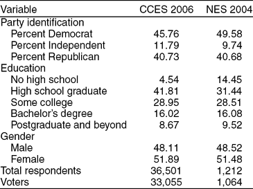
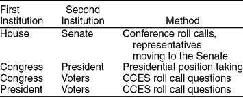
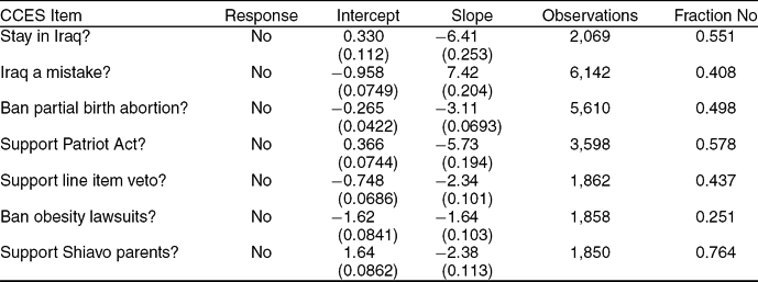
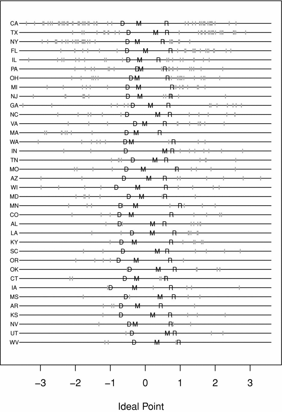
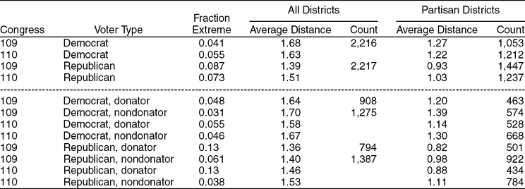
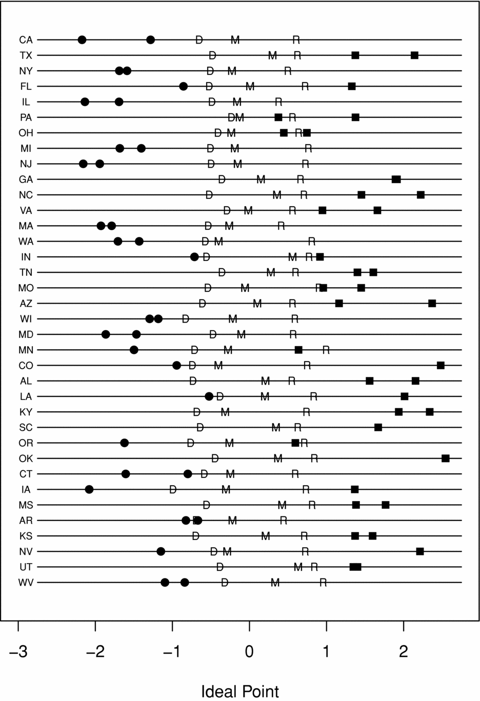
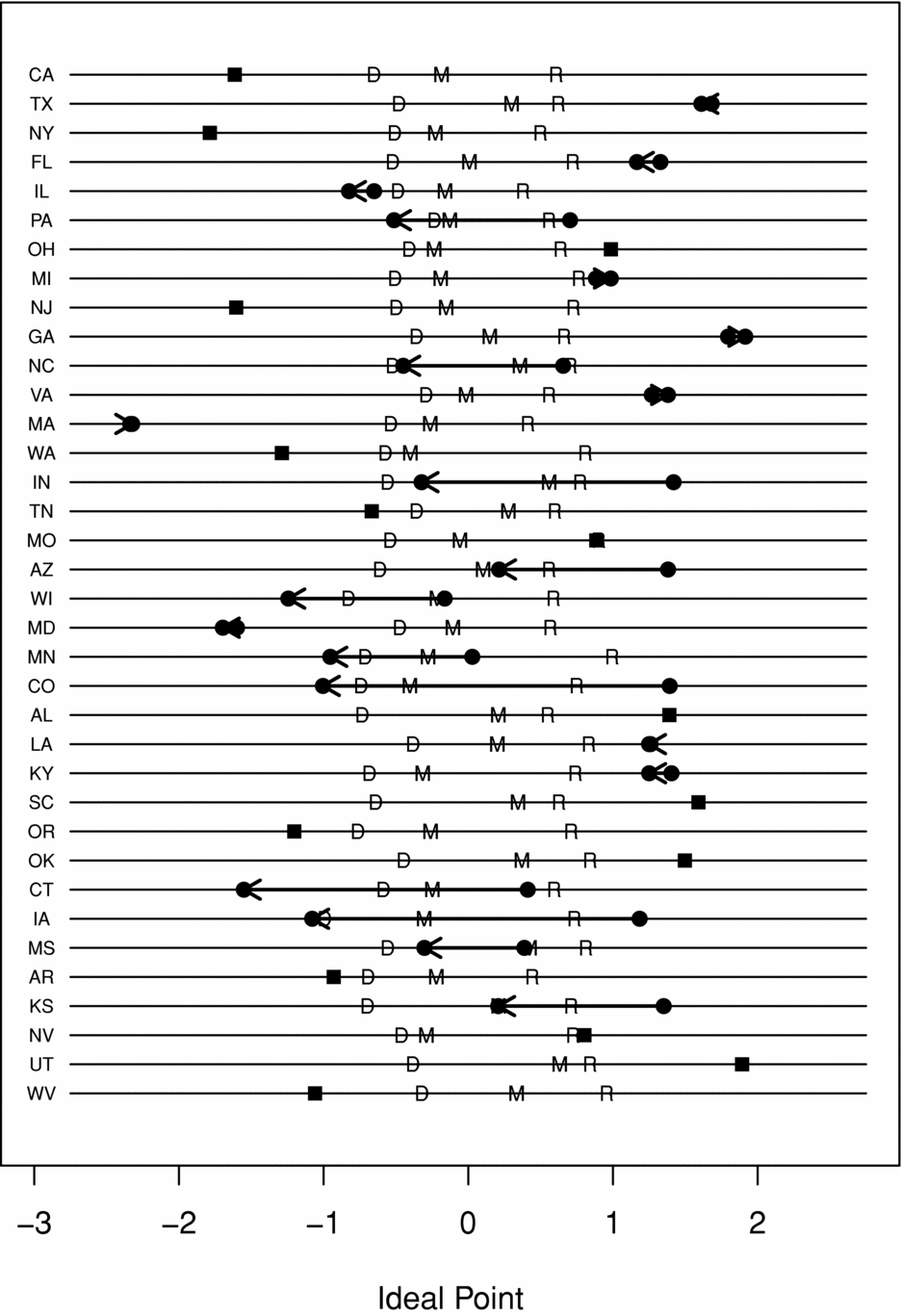
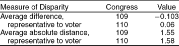
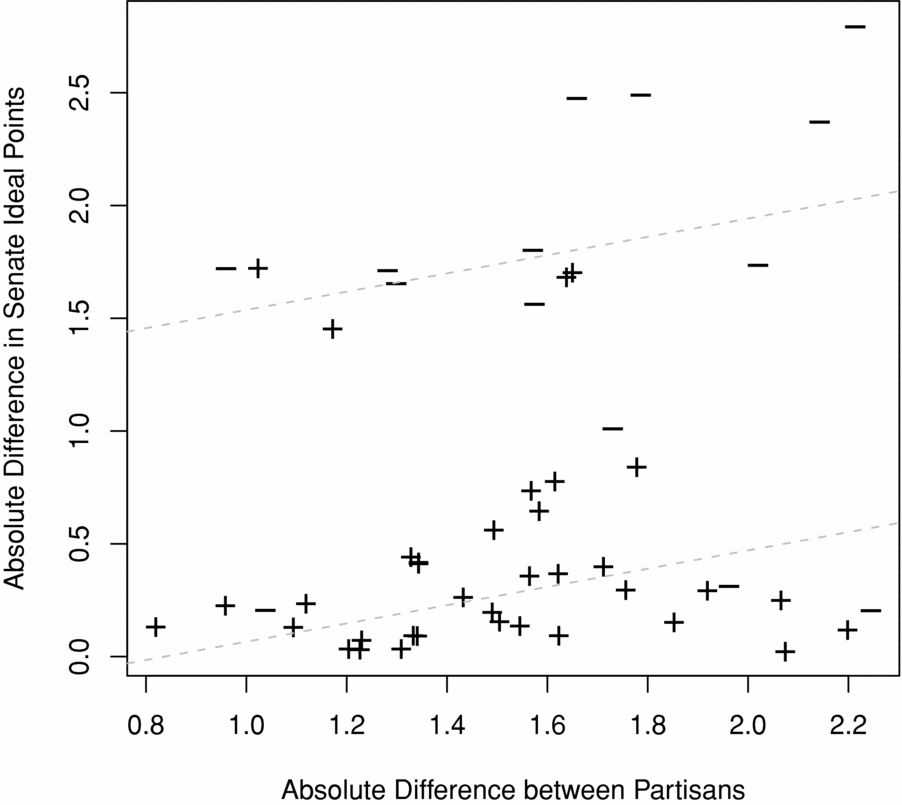
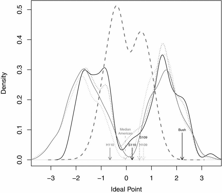
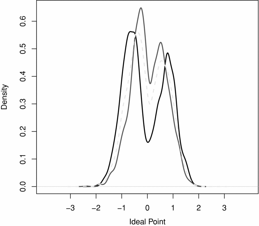
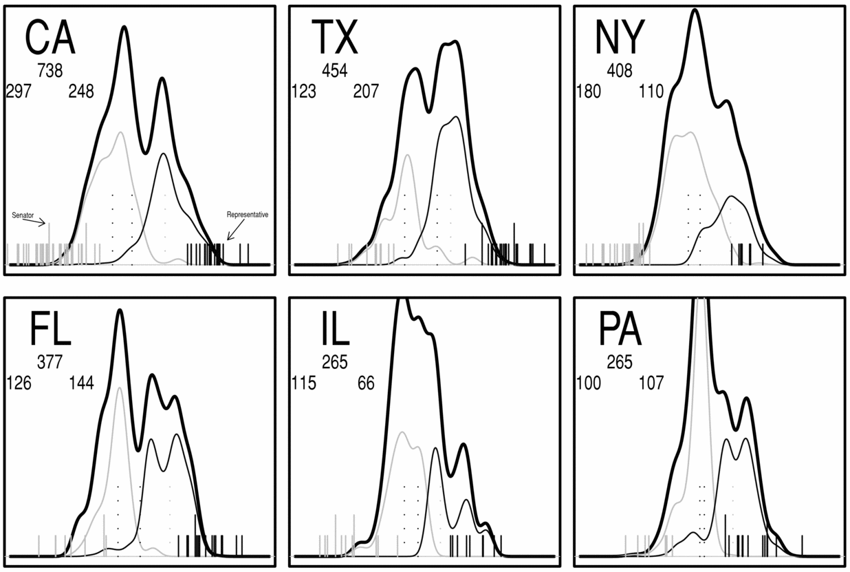




Comments
No Comments have been published for this article.