1 Introduction
The leading-edge boundary layer (LEBL) near the attachment line of swept airplane wings is subcritically unstable, i.e. it may undergo transition to turbulence substantially below the critical Reynolds number of linear stability theory. This instability is particularly important because turbulent flow emanating from the front part of a swept wing may contaminate large portions of the wing chord further downstream. Since this leads to substantially increased overall skin friction and thus airplane fuel consumption, the causes of this instability must be understood, such that concepts can be developed to maintain laminar flow. Even though the first observations of this LEBL instability and transition to turbulent flow were already made in the 1940s, no concise theoretical explanations are available to date. In this paper, we present one possible explanation for the subcritical transition in the LEBL, which may contribute to improved transition prediction, flow control and ultimately drag reduction.
It is common to employ the swept Hiemenz boundary layer (SHBL) past a flat plate (Rosenhead Reference Rosenhead1963; Schlichting Reference Schlichting1979) as a model for the LEBL (Pfenninger Reference Pfenninger1965; Gaster Reference Gaster1967) past a swept cylinder (Poll Reference Poll1979; Obrist Reference Obrist2000; John Reference John2014). Its instability was reported by Kuethe, McKee & Curry (Reference Kuethe, McKee and Curry1949), Gray (Reference Gray1952), Owen & Randall (Reference Owen and Randall1952) and Emslie, Hosking & Marshall (Reference Emslie, Hosking and Marshall1953) and was shown to be independent (Owen & Randall Reference Owen and Randall1952) of the previously known viscous, modal Tollmien–Schlichting-type instability along the chord of the airfoil described by Schubauer & Skramstad (Reference Schubauer and Skramstad1947). It was also shown to be different from the centrifugal instability (Taylor Reference Taylor1923) in the strongly accelerated front part where the cross-flow velocity component is strong (cf. Saric, Reed & White Reference Saric, Reed and White2003). Besides these experimental discoveries, a linear stability ansatz was developed (Görtler Reference Görtler, Görtler and Tollmien1955; Hämmerlin Reference Hämmerlin, Görtler and Tollmien1955), whose far-field solutions are hypergeometric functions (Obrist Reference Obrist2000). Numerous further experiments by Boltz, Kenyon & Allen (Reference Boltz, Kenyon and Allen1960), Pfenninger (Reference Pfenninger1965, Reference Pfenninger1977), Gaster (Reference Gaster1967), Cumpsty & Head (Reference Cumpsty and Head1969) and Poll (Reference Poll1978, Reference Poll1979) confirmed the validity of this Görtler–Hämmerlin (GH) ansatz and reported a linear critical Reynolds number
 $Re_{crit}\approx 580$
. Wilson & Gladwell (Reference Wilson and Gladwell1978) uncovered that the GH ansatz not only leads to modes which decay exponentially in the wall-normal direction, but that algebraically decaying modes exist as well (Dhanak & Stuart Reference Dhanak and Stuart1995; Obrist & Schmid Reference Obrist, Schmid, Schlatter and Henningson2010, Reference Obrist and Schmid2011). The direct solution of the stability equations by Hall, Malik & Poll (Reference Hall, Malik and Poll1984) resulted in a linear critical Reynolds number of
 $Re_{crit}\approx 583.1$
, which is in good agreement with the preceding experimental findings (Poll Reference Poll1979) and which was later confirmed by direct numerical simulations of Spalart (Reference Spalart1988).
However, transition is regularly observed in experiments above the significantly lower value
 $Re_{tr}\approx 250$
(Gaster Reference Gaster1967; Poll Reference Poll1979; Danks & Poll Reference Danks, Poll, Duck and Hall1995; Poll & Danks Reference Poll and Danks1995; Arnal et al.
Reference Arnal, Juillen, Reneaux and Gasparian1997), if the flow is subject to sufficiently large disturbances, as confirmed in the simulations by Spalart (Reference Spalart1988) and Dimas, Mowli & Piomelli (Reference Dimas, Mowli and Piomelli2003). Experiments by Gaster (Reference Gaster1967) and Pfenninger (Reference Pfenninger1977) led to the hypothesis of leading-edge contamination, i.e. an instability which requires for its triggering the advection of large disturbances or turbulent flow to the attachment line, e.g. from the fuselage–wing junction. Later, it was demonstrated that the SHBL as such can be subcritically unstable (Arnal, Perraud & Séraudie Reference Arnal, Perraud and Séraudie2009) and that transition along the leading edge may occur independently of the spanwise position along the wing (Gray Reference Gray1952; Arnal, Coustols & Juillen Reference Arnal, Coustols and Juillen1984; Kachanov & Moreau Reference Kachanov, Moreau, Duck and Hall1995). Obviously, a linear stability analysis of the SHBL cannot explain this subcritical transition.
For technical applications, it is important that wall suction is able to stabilize the flow. With
 ${\it\kappa}$
denoting its non-dimensional strength, wall suction is known to increase both the linear critical Reynolds number
 $Re_{crit}({\it\kappa})$
(Hall et al.
Reference Hall, Malik and Poll1984) and the transition Reynolds number
 $Re_{tr}({\it\kappa})$
(Spalart Reference Spalart1988; Danks & Poll Reference Danks, Poll, Duck and Hall1995; Poll & Danks Reference Poll and Danks1995; Arnal et al.
Reference Arnal, Juillen, Reneaux and Gasparian1997). This behaviour was linked to the linear stability theory of a broader class of homogeneous flat-plate boundary layers by John, Obrist & Kleiser (Reference John, Obrist and Kleiser2012, Reference John, Obrist and Kleiser2014a
). In particular, the SHBL with suction turns into the highly stable asymptotic suction boundary layer (ASBL) in the limit of vanishing chordwise flow, e.g. when increasing the sweep angle to
 $90^{\circ }$
. This approach also united the linear stability of the ASBL and the SHBL in a unified concept (John Reference John2014) and showed that the Görtler–Hämmerlin eigenmodes of the SHBL turn into the Tollmien–Schlichting eigenmodes of the ASBL in the respective parametric limit (John, Obrist & Kleiser Reference John, Obrist and Kleiser2015).
Several authors investigated the LEBL instability by going beyond classical linear stability analysis. Hall & Malik (Reference Hall and Malik1986) carried out a weakly nonlinear analysis, and Hall & Seddougui (Reference Hall and Seddougui1990) investigated the interaction of GH waves with oblique waves by using triple-deck theory. Neither work observed a substantial reduction of the critical Reynolds number. Theofilis (Reference Theofilis1998) investigated the stability of forced GH modes, which led to the same results as the classical analysis, concluding that only three-dimensional instabilities involving a dependence on the sweep direction may cause subcritical transition. Numerical simulations by Joslin (Reference Joslin1995) even observed damped disturbances of finite amplitude for Reynolds numbers slightly below the critical one, suggesting that the instability be supercritical. Linear stability theory was revisited with different extensions of the GH ansatz functions to elaborate chordwise polynomials by Theofilis (Reference Theofilis1993) and Obrist & Schmid (Reference Obrist and Schmid2003a
). However, both analyses resulted in the same value for the linear critical Reynolds number and the same most unstable GH mode. Furthermore, biglobal stability analyses of the SHBL were carried out by Lin & Malik (Reference Lin and Malik1996), Theofilis et al. (Reference Theofilis, Fedorov, Obrist and Dallmann2003) and Robitaillié-Montané (Reference Robitaillié-Montané2005). Unstable, travelling waves were identified, albeit only for Reynolds numbers above the classical value
 $Re_{crit}\approx 583.1$
. Even under an additional angle of attack, the GH mode reappears as the most unstable one (Pérez, Rodríguez & Theofilis Reference Pérez, Rodríguez and Theofilis2012). Further numerical simulations of the flow were carried out, which reconfirmed the results of linear theory (Theofilis Reference Theofilis1993). Obrist & Schmid (Reference Obrist and Schmid2003b
) and Schmid (Reference Schmid2007) investigated transient growth, but did not report any subcritical instability. Dimas et al. (Reference Dimas, Mowli and Piomelli2003) reported breakdown to turbulence at the marginally subcritical Reynolds number 570 in a large-eddy simulation (LES) with a quasi-turbulent inflow boundary condition. However, none of these approaches has led to a comprehensive explanation for transition observed at subcritical Reynolds numbers in the range of
 $250<Re<Re_{crit}$
.
Motivated by this discrepancy between linear stability results and experimental findings, Obrist, Henniger & Kleiser (Reference Obrist, Henniger and Kleiser2012) and John, Obrist & Kleiser (Reference John, Obrist and Kleiser2014b ) carried out DNS of the SHBL flow with an additional damped, primary disturbance of finite amplitude. These authors reported a bypass transition mechanism at subcritical Reynolds numbers, which can explain the occurrence of turbulence in experiments. The mechanism is based on a pair of steady streamwise vortices (primary perturbation), which lead to the transient growth of streaks due to the lift-up effect (Landahl Reference Landahl1980). These counter-rotating vortices are optimal disturbances in Falkner–Skan–Cooke boundary layers in general (Corbett & Bottaro Reference Corbett and Bottaro2001) and in the SHBL in particular (Guegan, Huerre & Schmid Reference Guegan, Huerre and Schmid2007; Guegan, Schmid & Huerre Reference Guegan, Schmid and Huerre2008). This damped primary perturbation (vortices and streaks) interacts with an unsteady secondary perturbation, yielding a secondary modal instability scenario.
Several studies have addressed similar secondary instability mechanisms in related flows. The secondary (symmetric or antisymmetric) instability of the Blasius boundary layer has been reported by Herbert (Reference Herbert1988) for superimposed finite-amplitude Tollmien–Schlichting waves and by Andersson et al. (Reference Andersson, Brandt, Bottaro and Henningson2001), Asai, Minagawa & Nishioka (Reference Asai, Minagawa and Nishioka2002), Brandt & Henningson (Reference Brandt and Henningson2002), Brandt (Reference Brandt2007), Duguet et al. (Reference Duguet, Schlatter, Henningson and Eckhardt2012) and Hack & Zaki (Reference Hack and Zaki2014) for superimposed vortex–streak configurations. The interaction of a saturated streak and a time-dependent disturbance is very effective in leading to transition, as demonstrated for Tollmien–Schlichting (TS) eigenmodes interacting with cross-flow disturbances (Bippes Reference Bippes, Arnal and Michel1989; Meyer & Kleiser Reference Meyer and Kleiser1989; Wintergerste & Kleiser Reference Wintergerste, Kleiser, Brommundt and Goerisch1995; Bippes Reference Bippes1999; Wintergerste Reference Wintergerste2002), for travelling cross-flow vortices (Wassermann & Kloker Reference Wassermann and Kloker2003) or for two streaks interacting with each other (Brandt & de Lange Reference Brandt and de Lange2008). Similarly, Görtler vortices were reported to grow slowly but to suffer from secondary instability when subject to a time-dependent disturbance (Park & Huerre Reference Park and Huerre1995).
The results of the current work may be linked to boundary-layer receptivity mechanisms which have been the subject of recent investigations. In this context, it is of interest that optimal perturbations in boundary layers were successfully connected to levels of free-stream turbulence (Matsubara & Alfredsson Reference Matsubara and Alfredsson2001), which might be generated at the fuselage. Alternatively, surface roughness or a wing–fuselage junction may generate perturbations in the boundary layer. While Fransson et al. (Reference Fransson, Brandt, Talamelli and Cossu2004) and White, Rice & Gökhan Ergin (Reference White, Rice and Gökhan Ergin2005) suggest that such perturbations do not have the character of optimal perturbations, they were shown to be even less stable than optimal ones and to exhibit secondary instability for lower streak amplitudes (Denissen & White Reference Denissen and White2013). Meneghello, Schmid & Huerre (Reference Meneghello, Schmid and Huerre2015) demonstrate that a strong receptivity is observed in particular for perturbations applied in the immediate vicinity of the attachment line. Finally, Thomas, Hall & Davies (Reference Thomas, Hall and Davies2015) report that wall suction significantly alters the receptivity of the cross-flow velocity in the swept Hiemenz flow.
In the present paper, we demonstrate that the SHBL disturbed by a class of primary, steady disturbances of finite amplitude may exhibit secondary instability. At the subcritical Reynolds numbers which we investigate, the SHBL is linearly stable, and all primary disturbances as such are damped. However, these primary disturbances may lead to secondary instability of the SHBL, i.e. we are able to find modally amplified secondary eigenmodes. We carry out a secondary stability analysis (SSA) to investigate this instability. Furthermore, this secondary instability may subsequently lead to transition to turbulent flow. We present DNS which illustrate the transition and breakdown to fully turbulent flow.
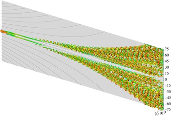
The remainder of this paper is structured as follows. Section 2 introduces the SHBL baseflow and the counter-rotating vortices which we superimpose to generate a primary, steady disturbance of finite amplitude. Section 3 presents a temporal secondary stability analysis of this secondary baseflow (cf. figure 1), which unveils an instability at Reynolds numbers as low as
 $Re\approx 175$
. Eigenspectra, eigenmodes and part of the stability diagram are presented in § 3.4. Section 4 reports DNS which confirm this secondary modal instability and which show breakdown to turbulent flow for Reynolds numbers as low as
 $Re=250$
. Section 4.4.3 compares the DNS results to those from SSA and § 4.4.4 to numerical and experimental results from the literature. Section 5 summarizes and concludes this paper.
2 Baseflow and governing equations
We carry out a biglobal linear SSA of the baseflow
 $\boldsymbol{u}_{B}$
which is obtained from a DNS based on the Navier–Stokes equation (NSE) for incompressible flow past an infinite swept plate. The coordinate system is described by
 $x$
in the chordwise,
 $y$
in the wall normal, and
 $z$
in the sweep direction. We call the sweep direction
 $z$
along the attachment line henceforth also the streamwise direction. We refer to
 $\boldsymbol{u}_{B}=\boldsymbol{u}_{SH}+\boldsymbol{u}_{1}^{\prime }$
as the secondary baseflow, which may be decomposed into the laminar SHBL flow
 $\boldsymbol{u}_{SH}$
(primary baseflow) and a primary disturbance
 $\boldsymbol{u}_{1}^{\prime }$
in the form of a three-dimensional vortex–streak system (VSS), as explained in the following two subsections. The flow
 $\boldsymbol{u}_{B}$
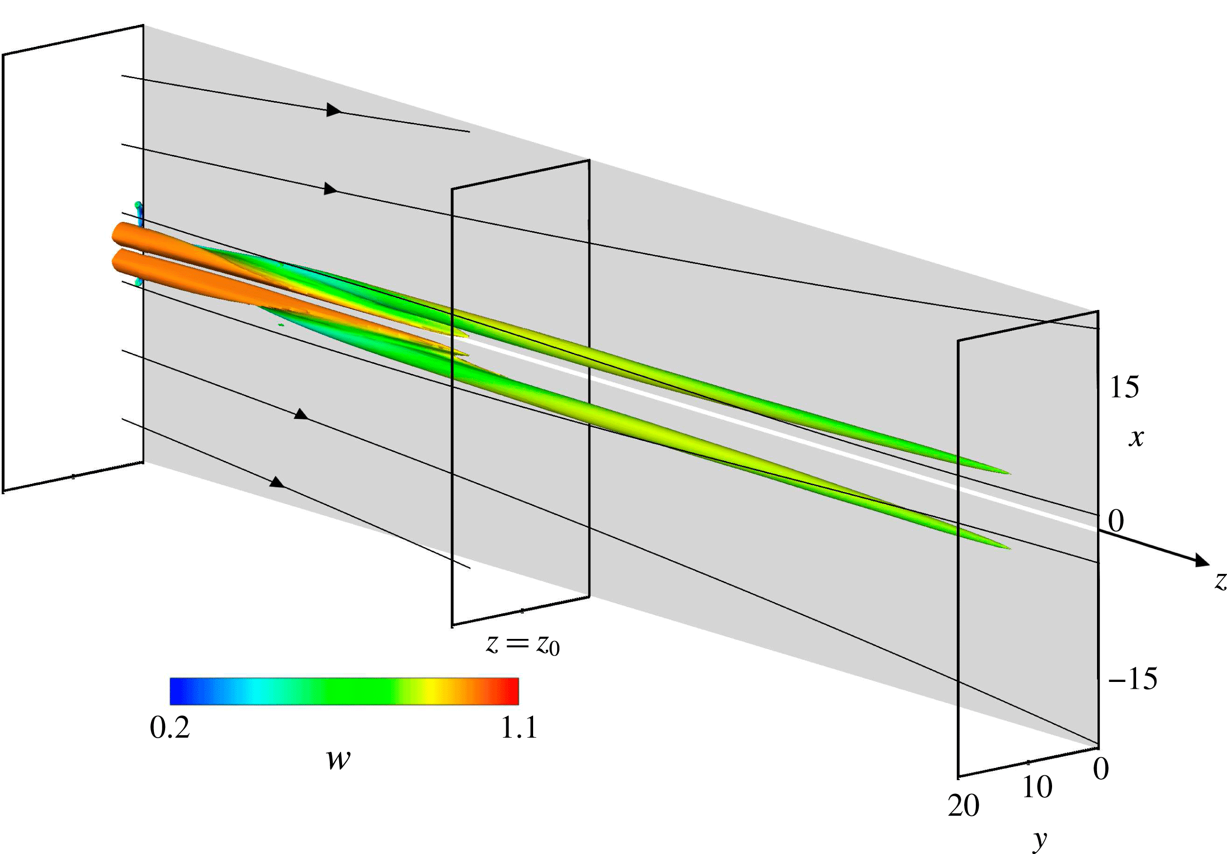
is illustrated in figure 1, from where we clearly see that the VSS is a damped three-dimensional disturbance of finite amplitude which slowly fades away in the downstream direction. Thus, we investigate the biglobal secondary stability (cf. Schmid & Henningson Reference Schmid and Henningson2001) of
 $\boldsymbol{u}_{B}$
. For the biglobal SSA in § 3, the baseflow
 $\boldsymbol{u}_{B}$
will be extracted from the DNS solution at some streamwise location
 $z_{0}$
(cf. figure 1), and the secondary eigenmodes
 $\boldsymbol{u}_{2}^{\prime }$
will be calculated from the secondary stability equations. For the DNS in § 4, a small secondary, time-dependent disturbance
 $\boldsymbol{u}_{2}^{\prime }$
is superimposed on
 $\boldsymbol{u}_{B}$
at the inflow boundary, which triggers the secondary instability and possibly subsequent transition.
Steady secondary baseflow
 $\boldsymbol{u}_{B}$
visualized by
 ${\it\lambda}_{2}$
isosurfaces, coloured by the local streamwise velocity component
 $w$
. The stability analysis of § 3 is carried out at some position
 $z=z_{0}$
.

2.1 Primary boundary-layer flow
 $\boldsymbol{u}_{SH}$

The classical SHBL is an extension of the plane stagnation boundary layer (Hiemenz Reference Hiemenz1911) with the assumption of an infinite swept plate (
 $\partial /\partial z=0$
). The non-dimensionalisation is based on the sweep velocity
 $W_{\infty }$
as the reference velocity and the standard reference length scale
 $\sqrt{{\it\nu}/a}$
, with the chordwise strain rate
 $a$
and the viscosity
 ${\it\nu}$
. Using the boundary-layer coordinate
 ${\it\eta}:=\sqrt{a/{\it\nu}}\times y$
, the ansatz for the velocity components
 $\boldsymbol{u}_{SH}$
,
 $\boldsymbol{v}_{SH}$
,
 $\boldsymbol{w}_{SH}$
in the
 $x$
-,
 $y$
- and
 $z$
-directions read
 $\boldsymbol{u}_{SH}(x,{\it\eta})=axf^{\prime }({\it\eta})$
,
 $\boldsymbol{v}_{SH}({\it\eta})=-\sqrt{a{\it\nu}}f({\it\eta})$
,
 $\boldsymbol{w}_{SH}({\it\eta})=W_{\infty }g({\it\eta})$
(e.g. Schlichting Reference Schlichting1979, p. 95). The components match the far-field
 $U(x,y)=ax$
,
 $V(x,y)=-ay$
,
 $W(x,y)=W_{\infty }$
for
 ${\it\eta}\rightarrow \infty$
. The self-similar functions
 $f$
and
 $g$
are determined from two ordinary differential equations obtained by substituting this ansatz into the NSE,
 $f^{\prime \prime \prime }+ff^{\prime \prime }-f^{\prime 2}+1=0$
and
 $g^{\prime \prime }+fg^{\prime }=0$
, subject to the boundary conditions
 $f(0)={\it\kappa}$
,
 $f^{\prime }(0)=0$
,
 $f^{\prime }({\it\eta}\rightarrow \infty )=1$
,
 $g(0)=0$
,
 $g({\it\eta}\rightarrow \infty )=1$
. At the wall, these boundary conditions impose the no-slip condition for the tangential velocity components
 $\boldsymbol{u}_{SH},\boldsymbol{w}_{SH}$
and account for a uniform wall-normal suction or injection velocity
 $\boldsymbol{v}_{SH}=-V_{0}$
. The non-dimensional suction strength is
 ${\it\kappa}=V_{0}/\sqrt{{\it\nu}a}$
, such that
 ${\it\kappa}=0$
represents a solid wall without suction. Even though the SHBL is referred to as a boundary-layer flow, it is not subject to any parallel flow assumption but rather an exact solution of the NSE.
2.2 Primary finite-amplitude disturbance
$\boldsymbol{u}_{1}^{\prime }$

By imposing two counter-rotating vortices on the SHBL
 $\boldsymbol{u}_{SH}$
as a Dirichlet boundary condition at the inflow plane
 $z=0$
, we generate a steady state, three-dimensional Navier–Stokes solution
 $\boldsymbol{u}_{B}$
. From
 $\boldsymbol{u}_{B}$
we subtract the SHBL
 $\boldsymbol{u}_{SH}$
to obtain the three-dimensional primary disturbance
 $\boldsymbol{u}_{1}^{\prime }$
. The vortex pair which we impose at
 $z=0$
is a generic model for three-dimensional disturbances that give rise to a horseshoe vortex near the leading edge, such as an isolated roughness element. Furthermore, these vortices are reminiscent of the optimal disturbances for the SHBL (Guegan et al.
Reference Guegan, Huerre and Schmid2007), leading to strong transient growth, and were shown to be highly unstable to secondary perturbations by Obrist et al. (Reference Obrist, Henniger and Kleiser2012). The vortices are aligned with the
 $z$
-direction at the inflow plane,
 $\boldsymbol{u}_{1}^{\prime }|_{z=0}=(\boldsymbol{u}_{1}^{\prime }(x,y),\boldsymbol{v}_{1}^{\prime }(x,y),0)^{\text{T}}$
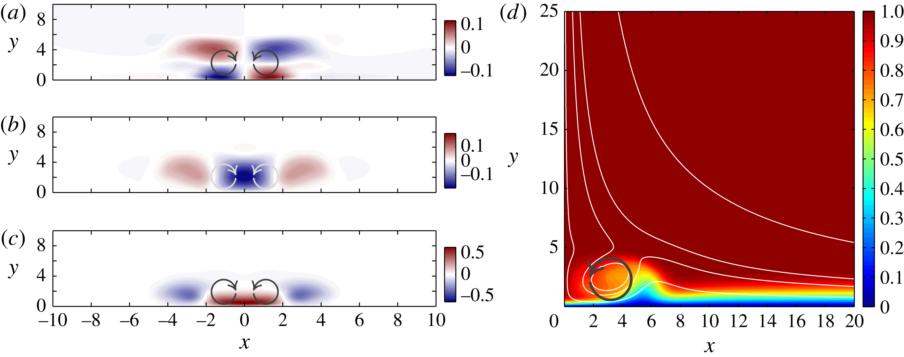
. Figure 2(a,b) illustrate
 $\boldsymbol{u}_{1}^{\prime }$
and
 $\boldsymbol{v}_{1}^{\prime }$
immediately downstream of the inflow plane
 $z=0$
. The vortex velocity components
 $u_{1}^{\prime }$
and
 $v_{1}^{\prime }$
on the inflow plane are parameterized by the primary disturbance amplitude
 $A_{1}$
, the centereline coordinates
 $x_{1}$
and
 $y_{1}$
and the radius
 $r_{1}$
(Obrist et al.
Reference Obrist, Henniger and Kleiser2012) as
 $$\begin{eqnarray}\displaystyle & \displaystyle u_{1}^{\prime }(x,y,z=0)=\frac{A_{1}}{2}\sin \frac{{\rm\pi}(y-y_{1})}{r_{1}}\left(\cos \frac{{\rm\pi}(x+x_{1})}{r_{1}}-\cos \frac{{\rm\pi}(x-x_{1})}{r_{1}}\right),~~~~\ & \displaystyle\end{eqnarray}$$
 $$\begin{eqnarray}\displaystyle & \displaystyle v_{1}^{\prime }(x,y,z=0)=\frac{A_{1}}{2}\left(1+\cos \frac{{\rm\pi}(y-y_{1})}{r_{1}}\right)\left(\sin \frac{{\rm\pi}(x-x_{1})}{r_{1}}-\sin \frac{{\rm\pi}(x+x_{1})}{r_{1}}\right),~~~~\ & \displaystyle\end{eqnarray}$$
 $|x-x_{1}|<r_{1}$
and
 $|y-y_{1}|<r_{1}$
, else
 $u_{1}^{\prime }|_{z=0}=v_{1}^{\prime }|_{z=0}=0$
.
(a–c) The three primary disturbance velocity components
 $\boldsymbol{u}_{1}^{\prime }$
at
 $z=14$
, (d) total streamwise velocity component
 $\boldsymbol{w}_{B}$
of the secondary baseflow (
 $\boldsymbol{w}_{SH}+\boldsymbol{w}_{1}^{\prime }$
) and sectional streamlines at
 $z=100$
. Arrows indicate the primary disturbance vortex orientation. (a)
 $\boldsymbol{u}_{1}^{\prime }(x,y)$
, (b)
 $\boldsymbol{v}_{1}^{\prime }(x,y)$
, (c)
 $\boldsymbol{w}_{1}^{\prime }(x,y)$
.

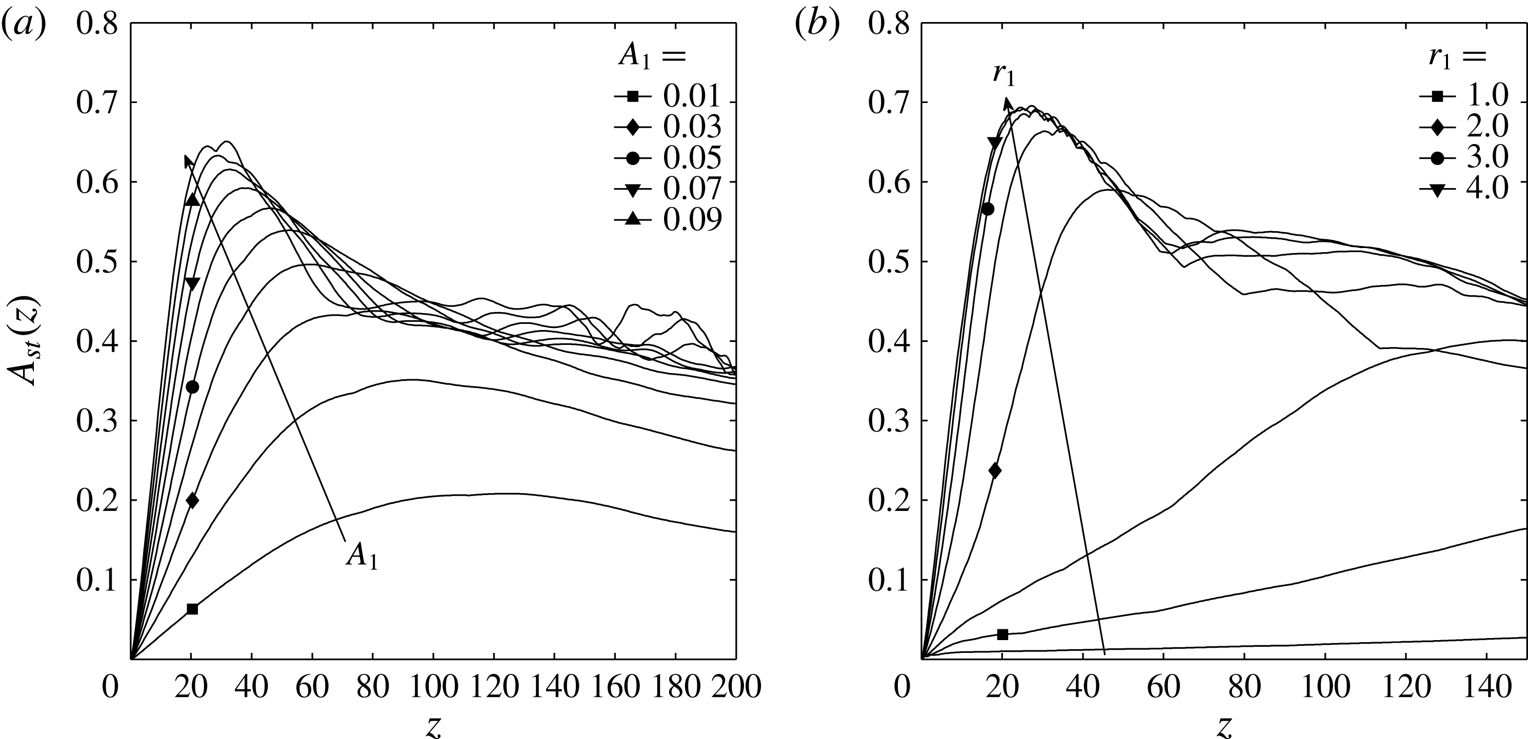
Streak amplitude
 $A_{st}(z)$
, (2.2), for various primary vortex configurations at large times. (a) Disturbance amplitudes
 $A_{1}=\{0.01,0.02,\ldots ,0.10\}$
,
 $r_{1}=3.0$
,
 $Re=300$
,
 ${\it\kappa}=0.0$
(secondary disturbance parameters
 $A_{2}=0.001$
,
 ${\it\omega}_{2}\approx 0.21$
). (b) Vortex radii
 $r_{1}=\{0.5,1.0,\ldots ,4.0\}$
,
 $A_{1}=0.10$
,
 $Re=500$
,
 ${\it\kappa}=0.2$
,
 $A_{2}=0$
.

The
 $w$
velocity component present in the SHBL
 $\boldsymbol{u}_{SH}$
advects this two-dimensional disturbance from the inflow plane
 $z=0$
into the computational domain. The vortices transport fluid of high streamwise momentum from the outer region towards the wall in the negative
 $y$
-direction (cf. figure 2
b), creating a high-speed streak (HSS) around the symmetry plane
 $x=0$
(cf. figure 2
c,d). Simultaneously, fluid of low streamwise momentum is advected from near the wall towards the outer regions of the boundary layer in the positive
 $y$
-direction, creating two low-speed streaks (LSS) at
 $x\approx \pm 2r_{1}$
(cf. figure 2
d). As a result, a three-dimensional VSS spreads along the attachment line throughout the computational domain. At the subcritical Reynolds numbers
 $Re<Re_{crit}$
investigated here, this VSS is a damped primary disturbance of the SHBL which decays slowly in the sweep direction
 $z$
(cf. figure 1). It is roughly oriented along the streamlines of the SHBL, such that the vortex core lines are increasingly tilted away from the attachment line as the flow proceeds downstream in the streamwise
 $z$
and chordwise
 $x$
-direction. In the absence of any secondary, time-dependent perturbation (
 $\boldsymbol{u}_{2}^{\prime }=0$
), the VSS leaves the computational domain as illustrated in figure 1 without becoming modally amplified or leading to transition. This HSS configuration is connected with vortices supported by the cross-flow situation for larger chordwise
 $x$
positions downstream. It is therefore unstable at much lower Reynolds numbers than an LSS configuration with an inverted sense of rotation of the vortex pair (John, Obrist & Kleiser Reference John, Obrist and Kleiser2016).
The strength of the VSS is a function of the primary disturbance parameters
 $x_{1}$
,
 $y_{1}$
,
 $r_{1}$
, and
 $A_{1}$
imposed at the inflow plane
 $z=0$
, and is measured (Andersson et al.
Reference Andersson, Brandt, Bottaro and Henningson2001) by the streak amplitude it generates,
 $$\begin{eqnarray}A_{st}(z,t;Re,{\it\kappa},A_{1},r_{1},\ldots )={\textstyle \frac{1}{2}}(\max _{x,y}w^{\prime }-\min _{x,y}w^{\prime }).\end{eqnarray}$$
Even though
 $A_{st}$
measures the total disturbance amplitude and thus is a function of both
 $z$
and
 $t$
, it becomes a quasi-time-independent measure
 $A_{st}(z)$
in the upstream regions of the domain where the steady primary streaks are dominant.
Figure 3 illustrates the influence of
 $A_{1}$
and
 $r_{1}$
on
 $A_{st}(z)$
observed in different secondary baseflows. The amplitude of the VSS grows transiently (Landahl Reference Landahl1980) in the streamwise
 $z$
-direction until saturation. Neither increasing
 $A_{1}$
beyond 0.1 nor increasing
 $r_{1}$
beyond
 $3.0$
does lead to significantly higher values of
 $A_{st}$
. Therefore, in the following, the disturbance parameters
 $A_{1}=0.1$
and
 $r_{1}=3.0$
are employed to generate the secondary baseflows unless noted otherwise.
The other primary disturbance parameters are set to
 $x_{1}=1.5$
,
 $y_{1}=3.0$
for all of the simulations presented in the following, which is the parameter combination where the streak amplitude
 $A_{st}$
and the location
 $z_{max}$
where the latter attains its maximum exhibit the lowest sensitivity. At the same time, these values are also effective in the sense that they lead to a rapid streak development and high streak amplitude (John Reference John2014).
3 Secondary biglobal stability analysis
In this section, we carry out a biglobal SSA of the secondary baseflow
 $\boldsymbol{u}_{B}$
by solving the temporal stability equations. We obtain eigenspectra and various eigenmodes with associated growth rates.
3.1 Two-dimensional baseflow for SSA
The baseflow
 $\boldsymbol{u}_{B}(x,y)=(\boldsymbol{u}_{B},\boldsymbol{v}_{B},\boldsymbol{w}_{B})^{\text{T}}$
is a three component, two-variate flow, which we extract from our three-dimensional DNS flow
 $\boldsymbol{u}_{DNS}$
at one particular location
 $z_{0}=100$
,
 $\boldsymbol{u}_{B}=\boldsymbol{u}_{DNS}(x,y,z=z_{0})$
. Even though any baseflow
 $\boldsymbol{u}_{B}$
obtained in this manner does not fulfil the two-dimensional continuity equation
 $\unicode[STIX]{x1D60B}_{x}\boldsymbol{u}_{B}=-\unicode[STIX]{x1D60B}_{y}\boldsymbol{v}_{B}$
identically (where
 $\unicode[STIX]{x1D60B}_{i}$
denotes the derivative in the
 $x_{i}$
-direction) this approximation is justified as follows. The idealization represents the analogy to the parallel flow assumption commonly used for nearly parallel, two-dimensional flows. It also applies to our three-dimensional flow because
 $\boldsymbol{u}_{DNS}$
may be decomposed into the primary SHBL baseflow
 $\boldsymbol{u}_{SH}$
and nonlinear primary disturbances
 $\boldsymbol{u}_{1}^{\prime }$
(cf. § 2). The former is invariant in the
 $z$
-direction and hence identically fulfils the two-dimensional continuity equation in
 $z=\text{const.}$
planes. Thus, only the very small primary disturbance gradients in the sweep direction,
 $\unicode[STIX]{x1D60B}_{z}\boldsymbol{w}_{1}^{\prime }$
, are neglected. The averaged streamwise divergence of the primary disturbance,
 $$\begin{eqnarray}\frac{1}{L_{x}L_{y}}\int _{0}^{L_{x}}\int _{0}^{L_{y}}\unicode[STIX]{x1D60B}_{z}\boldsymbol{w}_{B}(x,y)|_{z=z_{0}}\,\text{d}y\,\text{d}x=\frac{1}{L_{x}L_{y}}\int _{0}^{L_{x}}\int _{0}^{L_{y}}\unicode[STIX]{x1D60B}_{z}\boldsymbol{w}_{1}^{\prime }(x,y)|_{z=z_{0}}\,\text{d}y\,\text{d}x\approx 10^{-4},\end{eqnarray}$$
is orders of magnitude smaller than typical values of
 $\unicode[STIX]{x1D60B}_{y}\boldsymbol{v}_{1}^{\prime }$
and
 $\unicode[STIX]{x1D60B}_{x}\boldsymbol{u}_{1}^{\prime }$
(see figure 2
a,b). Therefore, we use the unaltered
 $\boldsymbol{u}_{B}$
and
 $\boldsymbol{v}_{B}$
velocity profiles obtained from DNS for our calculations.
Obviously, the choice of the extraction location
 $z_{0}=100$
may have some influence on the baseflow profile
 $\boldsymbol{u}_{B}(x,y)=\boldsymbol{u}_{DNS}(x,y,z=z_{0})$
. However, tests have shown that a modification of
 $z_{0}$
in the vicinity of the location where (3.1) attains its minimum (
 $z_{0}\approx 100$
) affects the results only very little (see John Reference John2014).
3.2 Secondary biglobal stability equations
We are interested in the stability of the secondary baseflow
 $\boldsymbol{u}_{B}$
. The ansatz for the secondary biglobal eigenmode
 $\boldsymbol{u}_{2}^{\prime }$
is a bivariate function of
 $x$
and
 $y$
and a travelling wave in the
 $z$
-direction. The stability equations are then obtained by linearizing the NSE about the secondary baseflow. Taking the curl of the NSE and substituting the baseflow vorticity
 ${\it\bf\Omega}_{B}=(\unicode[STIX]{x1D60B}_{y}\boldsymbol{w}_{B},-\unicode[STIX]{x1D60B}_{x}\boldsymbol{w}_{B},\unicode[STIX]{x1D60B}_{x}\boldsymbol{v}_{B}-\unicode[STIX]{x1D60B}_{y}\boldsymbol{v}_{B})^{\text{T}}$
and the modal ansatz
 $$\begin{eqnarray}\boldsymbol{u}_{2}^{\prime }={\textstyle \frac{1}{2}}[(\hat{\boldsymbol{u}}(x,y),\hat{\boldsymbol{v}}(x,y),\hat{\boldsymbol{v}}(x,y))^{\text{T}}\exp (\text{i}{\it\gamma}(z-ct))+\text{c.c.}]\end{eqnarray}$$
leads to the equations of linear secondary biglobal instability
 $$\begin{eqnarray}\displaystyle & & \displaystyle (\text{i}{\it\gamma}c+\mathscr{L}-\unicode[STIX]{x1D60B}_{y}\boldsymbol{v}_{B})((\unicode[STIX]{x1D60B}_{y}^{2}-{\it\gamma}^{2})\hat{\boldsymbol{v}}+\unicode[STIX]{x1D60B}_{x}\unicode[STIX]{x1D60B}_{y}\hat{\boldsymbol{u}})=(-\text{i}{\it\gamma}\unicode[STIX]{x1D60B}_{y}^{2}\boldsymbol{w}_{B}+\unicode[STIX]{x1D60B}_{y}\boldsymbol{u}_{B}\unicode[STIX]{x1D60B}_{x}\unicode[STIX]{x1D60B}_{y})\hat{\boldsymbol{v}}\nonumber\\ \displaystyle & & \displaystyle \quad +\,(-\unicode[STIX]{x1D60B}_{x}\unicode[STIX]{x1D60B}_{y}\boldsymbol{w}_{B}\text{i}{\it\gamma}+\unicode[STIX]{x1D60B}_{y}\boldsymbol{w}_{B}\unicode[STIX]{x1D60B}_{x}\text{i}{\it\gamma}-\unicode[STIX]{x1D60B}_{x}\boldsymbol{w}_{B}\unicode[STIX]{x1D60B}_{y}\text{i}{\it\gamma}+\unicode[STIX]{x1D60B}_{y}\boldsymbol{u}_{B}\unicode[STIX]{x1D60B}_{x}^{2}-{\it\gamma}^{2}\unicode[STIX]{x1D60B}_{x}\boldsymbol{v}_{B})\hat{\boldsymbol{u}},\end{eqnarray}$$
 $$\begin{eqnarray}\displaystyle & & \displaystyle (\text{i}{\it\gamma}c+\mathscr{L}+\unicode[STIX]{x1D60B}_{y}\boldsymbol{v}_{B})((\unicode[STIX]{x1D60B}_{x}^{2}-{\it\gamma}^{2})\hat{\boldsymbol{u}}+\unicode[STIX]{x1D60B}_{x}\unicode[STIX]{x1D60B}_{y}\hat{\boldsymbol{v}})=(-\text{i}{\it\gamma}\unicode[STIX]{x1D60B}_{x}^{2}\boldsymbol{w}_{B}+\unicode[STIX]{x1D60B}_{x}\boldsymbol{v}_{B}\unicode[STIX]{x1D60B}_{x}\unicode[STIX]{x1D60B}_{y})\hat{\boldsymbol{u}}\nonumber\\ \displaystyle & & \displaystyle \quad +\,(-\unicode[STIX]{x1D60B}_{x}\unicode[STIX]{x1D60B}_{y}\boldsymbol{w}_{B}\text{i}{\it\gamma}-\unicode[STIX]{x1D60B}_{y}\boldsymbol{w}_{B}\unicode[STIX]{x1D60B}_{x}\text{i}{\it\gamma}+\unicode[STIX]{x1D60B}_{x}\boldsymbol{w}_{B}\unicode[STIX]{x1D60B}_{y}\text{i}{\it\gamma}+\unicode[STIX]{x1D60B}_{x}\boldsymbol{v}_{B}\unicode[STIX]{x1D60B}_{y}^{2}-{\it\gamma}^{2}\unicode[STIX]{x1D60B}_{y}\boldsymbol{u}_{B})\hat{\boldsymbol{v}},\end{eqnarray}$$
 $$\begin{eqnarray}\mathscr{L}\equiv {\rm\nabla}^{2}/Re-(\boldsymbol{u}_{B}\unicode[STIX]{x1D60B}_{x}+\boldsymbol{v}_{B}\unicode[STIX]{x1D60B}_{y}+\boldsymbol{w}_{B}\text{i}{\it\gamma}),\quad {\rm\nabla}^{2}\equiv \unicode[STIX]{x1D60B}_{x}^{2}+\unicode[STIX]{x1D60B}_{y}^{2}-{\it\gamma}^{2}.\end{eqnarray}$$
We investigate temporal instability, thus
 ${\it\gamma}\in \mathbb{R}$
is a real wavenumber and the phase speed and growth rate of each mode are described by
 $c=c_{r}+\text{i}c_{i}\in \mathbb{C}$
. Equations (3.3) are subject to the eight (physical) boundary conditions
 $\hat{\boldsymbol{u}}=\hat{\boldsymbol{v}}=0$
for
 $\{x\rightarrow \pm \infty ,y=0,y\rightarrow \infty \}$
. In practice, these conditions need to be transformed to numerical boundary conditions which are applied to the discretized system on a truncated domain
 $x\in [-L_{x},L_{x}]$
,
 $y\in [0,L_{y}]$
. Furthermore, for the present symmetric baseflow, (3.3) may be reformulated, enforcing groups of either symmetric (
 $s$
) or antisymmetric (
 $a$
) modes with respect to
 $x=0$
(cf. Obrist Reference Obrist2000). Therefore, the size of the numerical domain may be reduced from
 $x\in [-L_{x},L_{x}]$
to
 $x\in [0,L_{x}]$
, a factor of two, at the complication of having to solve (3.3) twice (for even/odd modes). When exploiting this symmetry property, the six boundary conditions imposed at
 $\{x\rightarrow \infty ,y=0,y\rightarrow \infty \}$
may be retained. The two remaining conditions at
 $x\rightarrow -\infty$
must be replaced by four symmetry conditions at
 $x=0$
because the order of the system (3.3) is four for (3.3a
) and (3.3b
). Together, this leads to the ten numerical boundary conditions
 $$\begin{eqnarray}\displaystyle & \hat{\boldsymbol{u}}=\hat{\boldsymbol{v}}=0\quad x=L_{x}, & \displaystyle\end{eqnarray}$$
 $$\begin{eqnarray}\displaystyle & \text{either}\quad \unicode[STIX]{x1D60B}_{x}\hat{\boldsymbol{u}}=\unicode[STIX]{x1D60B}_{xxx}\hat{\boldsymbol{u}}=\hat{\boldsymbol{v}}=\unicode[STIX]{x1D60B}_{xx}\hat{\boldsymbol{v}}=0\quad x=0~(a) & \displaystyle\end{eqnarray}$$
 $$\begin{eqnarray}\displaystyle & \text{or}\quad \hat{\boldsymbol{u}}=\unicode[STIX]{x1D60B}_{xx}\hat{\boldsymbol{u}}=\unicode[STIX]{x1D60B}_{x}\hat{\boldsymbol{v}}=\unicode[STIX]{x1D60B}_{xxx}\hat{\boldsymbol{v}}=0\quad x=0,~(s) & \displaystyle\end{eqnarray}$$
 $$\begin{eqnarray}\displaystyle & \hat{\boldsymbol{u}}=\hat{\boldsymbol{v}}=0\quad y=0,L_{y}. & \displaystyle\end{eqnarray}$$
 $L_{x}$
and
 $L_{y}$
are chosen ad hoc such that numerical convergence is reached (cf. John Reference John2014).
3.3 Numerical solution method
Equations (3.3)–(3.5) form a generalized eigenvalue problem for
 $\hat{\boldsymbol{u}}$
and
 $\hat{\boldsymbol{v}}$
of the form
 $$\begin{eqnarray}\left[\begin{array}{@{}cc@{}}\unicode[STIX]{x1D617}_{uu} & \unicode[STIX]{x1D617}_{uv}\\ \unicode[STIX]{x1D617}_{vu} & \unicode[STIX]{x1D617}_{vv}\end{array}\right]\left[\begin{array}{@{}c@{}}\hat{\boldsymbol{u}}(x,y)\\ \hat{\boldsymbol{v}}(x,y)\end{array}\right]=c\left[\begin{array}{@{}cc@{}}\unicode[STIX]{x1D618}_{uu} & \unicode[STIX]{x1D618}_{uv}\\ \unicode[STIX]{x1D618}_{vu} & \unicode[STIX]{x1D618}_{vv}\end{array}\right]\left[\begin{array}{@{}c@{}}\hat{\boldsymbol{u}}(x,y)\\ \hat{\boldsymbol{v}}(x,y)\end{array}\right].\end{eqnarray}$$
The eigenfunctions
 $\hat{\boldsymbol{u}}$
and
 $\hat{\boldsymbol{v}}$
are discretized on an
 $N_{x}\times N_{y}$
grid as vectors of size
 $\hat{\boldsymbol{u}},\hat{\boldsymbol{v}}\in \mathbb{C}^{(NxNy)\times 1}$
. Grid stretching is employed in the
 $x$
- and
 $y$
-directions according to
 $$\begin{eqnarray}x_{i}=x_{i,h}\left(\frac{1+{\it\xi}}{1-{\it\xi}/A}\right),\quad A=\frac{L_{i}}{L_{i}-2x_{i,h}+{\it\epsilon}},\end{eqnarray}$$
with
 ${\it\xi}\in [-1,1]$
distributed uniformly. This results in 50 % of the points being concentrated within the intervals
 $x_{i}\in [0,x_{i,h}]$
. The values chosen for the present calculations are
 $L_{x}=20$
,
 $x_{h}=20/3$
in the chordwise
 $x$
-direction and
 $L_{y}=25$
,
 $y_{h}=5$
in the wall-normal
 $y$
-direction. The number of grid points is
 $N_{x}=150$
,
 $N_{y}=120$
for which grid convergence is reached for wavenumbers
 ${\it\gamma}\gtrapprox 0.5$
. The eight sparse submatrices
 $\unicode[STIX]{x1D617}_{ij},\unicode[STIX]{x1D618}_{ij}$
, each of dimension
 $\mathbb{C}^{(NxNy)\times (NxNy)}$
, are set up separately. The first and second derivatives in the
 $x$
- and
 $y$
-directions are provided by central finite differences of fourth order. The stencil is one sided at boundary points. The derivatives of higher order are constructed by multiplication of the matrices for the first and second derivatives. The matrices
 $\unicode[STIX]{x1D64B}$
and
 $\unicode[STIX]{x1D64C}$
are given in the appendix A. The boundary conditions (3.5) are applied to each of the submatrices
 $\unicode[STIX]{x1D617}_{ij},\unicode[STIX]{x1D618}_{ij}$
before the operator matrices
 $\unicode[STIX]{x1D64B}$
and
 $\unicode[STIX]{x1D64C}$
are assembled. The built-in MATLAB function eigs is employed to solve (3.6) for the eigenvalue
 $c$
and eigenfunctions
 $\hat{\boldsymbol{u}}$
and
 $\hat{\boldsymbol{v}}$
in an iterative manner using a standard Krylov-subspace Arnoldi method (Trefethen & Bau Reference Trefethen and Bau1997). The run time for the eigenvalue solver is small compared to the time required to set up the matrices
 $\unicode[STIX]{x1D64B},\unicode[STIX]{x1D64C}$
. Therefore, we apply the Arnoldi algorithm five times with different initial guesses
 $c_{0}$
to efficiently investigate a large portion of the eigenspectrum. Identical modes resulting from different initial guesses
 $c_{0}$
are deleted during post-processing. For further details, such as convergence studies, we refer to John (Reference John2014).
3.4 Results
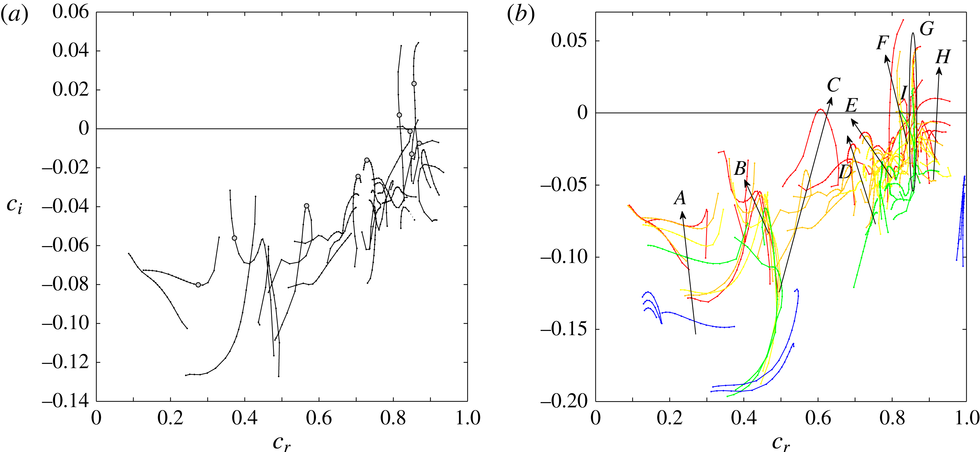
A typical secondary eigenspectrum of antisymmetric (
 $a$
) modes (cf. (3.5c
)) for
 $Re=400$
and a broad range of wavenumbers
 ${\it\gamma}$
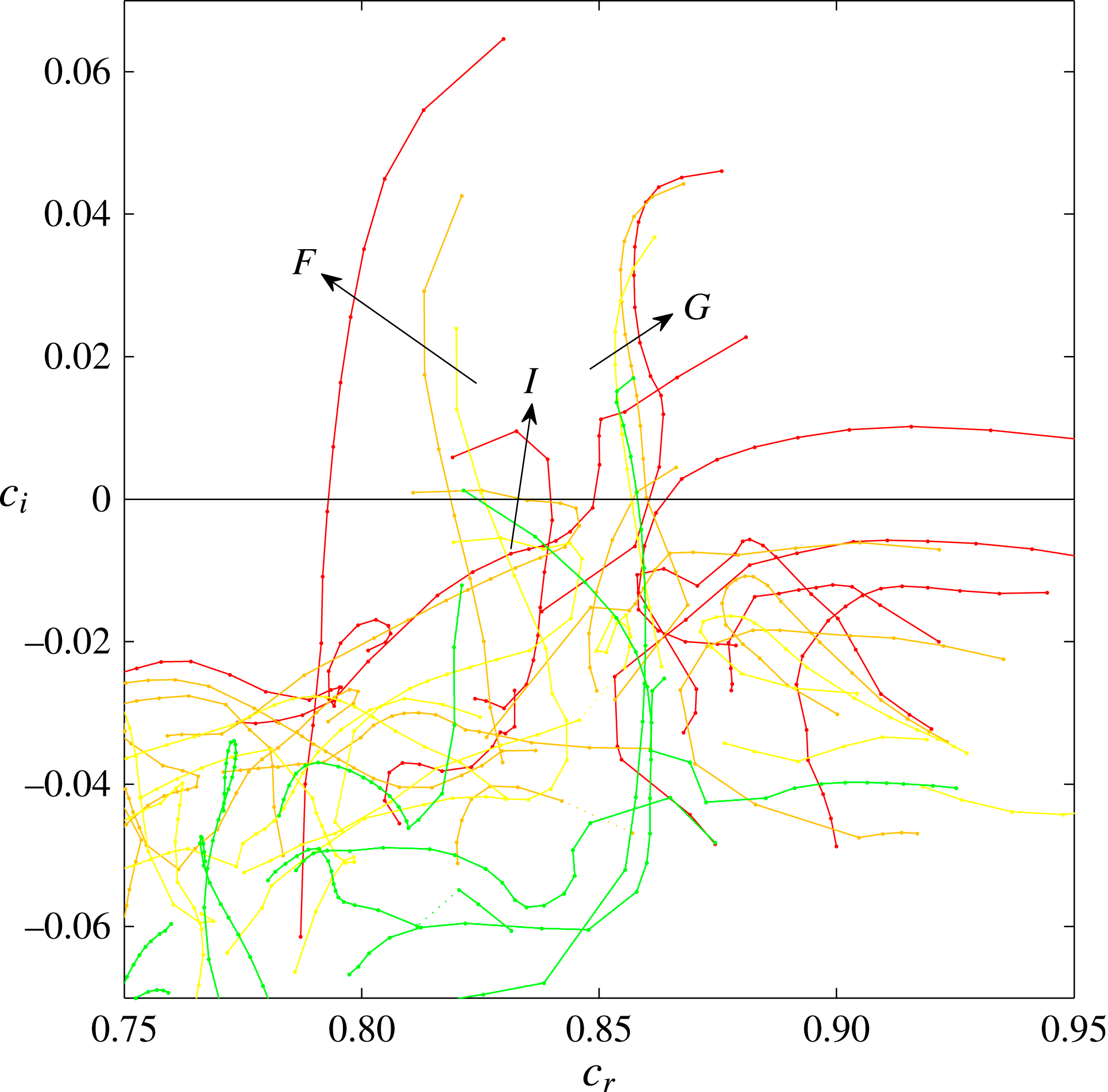
is illustrated in figure 4(a). Ten branches are observed in different regions of phase speed
 $c_{r}$
as
 ${\it\gamma}$
is varied. A large number of only weakly damped modes (branches
 $A$
,
 $B$
,
 $D$
,
 $E$
in figure 4
b) and several amplified eigenmodes (branches
 $C$
,
 $F$
,
 $G$
,
 $H$
,
 $I$
) are observed at this subcritical Reynolds number.
(a) A typical secondary eigenspectrum of antisymmetric modes obtained for
 $Re=400$
,
 ${\it\kappa}=0$
,
 ${\it\gamma}\in [0.5,5.0]$
. (b) Eigenspectra of secondary antisymmetric instability for
 $Re\in \{100,200,300,400,500\}$
(colour sequence: blue, green, yellow, orange, red) and
 ${\it\gamma}\in [0.5,5.0]$
(branches),
 ${\it\kappa}=0$
. An enlargement of (b) is illustrated in figure 5.

3.4.1 Branches of modes for varying wavenumbers
Figure 4(b) shows spectra for different Reynolds numbers
 $Re$
, in addition to the variation of
 ${\it\gamma}$
. A number of modally growing or weakly damped modes cover a large portion of the spectrum already at very low Reynolds numbers. Branch
 $G$
(green) is unstable already at
 $Re=200$
, far below
 $Re_{crit}\approx 583.1$
. For
 $Re=500$
the number of amplified modes is already large. The upper right region of the spectrum is enlarged in figure 5.
Closeup of figure 4(b): eigenspectra of secondary antisymmetric instability for
 $Re\in \{200,300,400,500\}$
(colour: green, yellow, orange, red) and
 ${\it\gamma}\in [0.5,5.0]$
(branches),
 ${\it\kappa}=0$
.

Six selected normalized secondary eigenmode velocity magnitudes
 $|\hat{\boldsymbol{w}}(x,y)|$
highlighted by circles on the antisymmetric branches depicted in figure 4(a). Red indicates regions of high velocity magnitude
 $|\hat{\boldsymbol{w}}|$
. The white curves are sectional streamlines of the secondary baseflow
 $\boldsymbol{u}_{B}$
. The branches and wavenumbers illustrated are (a)
 $A$
,
 ${\it\gamma}=0.9$
, (b)
 $B$
,
 ${\it\gamma}=0.8$
, (c)
 $D$
,
 ${\it\gamma}=2.5$
, (d)
 $E$
,
 ${\it\gamma}=2.5$
, (e)
 $F$
,
 ${\it\gamma}=0.8$
, (f)
 $I$
,
 ${\it\gamma}=0.9$
.
 $Re=400$
,
 ${\it\kappa}=0$
. Colour bar see figure 2.

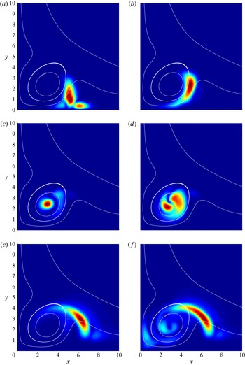
Six of the ten eigenmodes highlighted in figure 4(a) are illustrated in figure 6. Some of them have substantial amplitudes in the lower shear layer close to the wall (a,b), in the vortex core (c,d) or in the upper, outer shear layer (e,f). Altogether, they cover a large portion of the boundary layer in the vicinity of the primary vortex and a broad region of phase speeds
 $c_{r}$
(cf. figure 4). Numerous modes are only weakly damped, and their similar geometric shape likely makes these modes a good basis for strong transient energy growth for a broad range of generic secondary disturbances.
The numerically converged eigenvalues illustrated in figure 4 do not change when the initial guess
 $c_{0}$
for the Arnoldi algorithm is altered. Likewise, the eigenvalues which constitute the branches do not jump discontinuously from one point in the spectrum to another when the grid resolution is altered. Rather, they smoothly converge when the grid resolution is increased. Furthermore, the exponential decay rate of all reported modes is proportional to
 $\exp (-{\it\gamma}y)$
and
 $\exp (-{\it\gamma}x)$
in the wall normal and chordwise directions. Thus, we conclude that the branches shown in figure 4 are formed by genuine discrete eigenmodes of the secondary baseflow
 $\boldsymbol{u}_{B}$
.
Dependence of the eigenmode of branch
 $C$
(cf. figure 4
b) on the wave number
 ${\it\gamma}$
,
 $Re=400$
,
 ${\it\kappa}=0$
. (a)
 ${\it\gamma}=0.50$
, (b) 0.60, (c) 0.70, (d) 0.80, (e) 0.90, (f) 1.00, (g) 1.10, (h) 1.20, (i) 1.30, (j) 1.40, (k) 1.50, (l) 1.60, (m) 1.80 (n) 2.00, (o) 2.50, (p) 3.00.

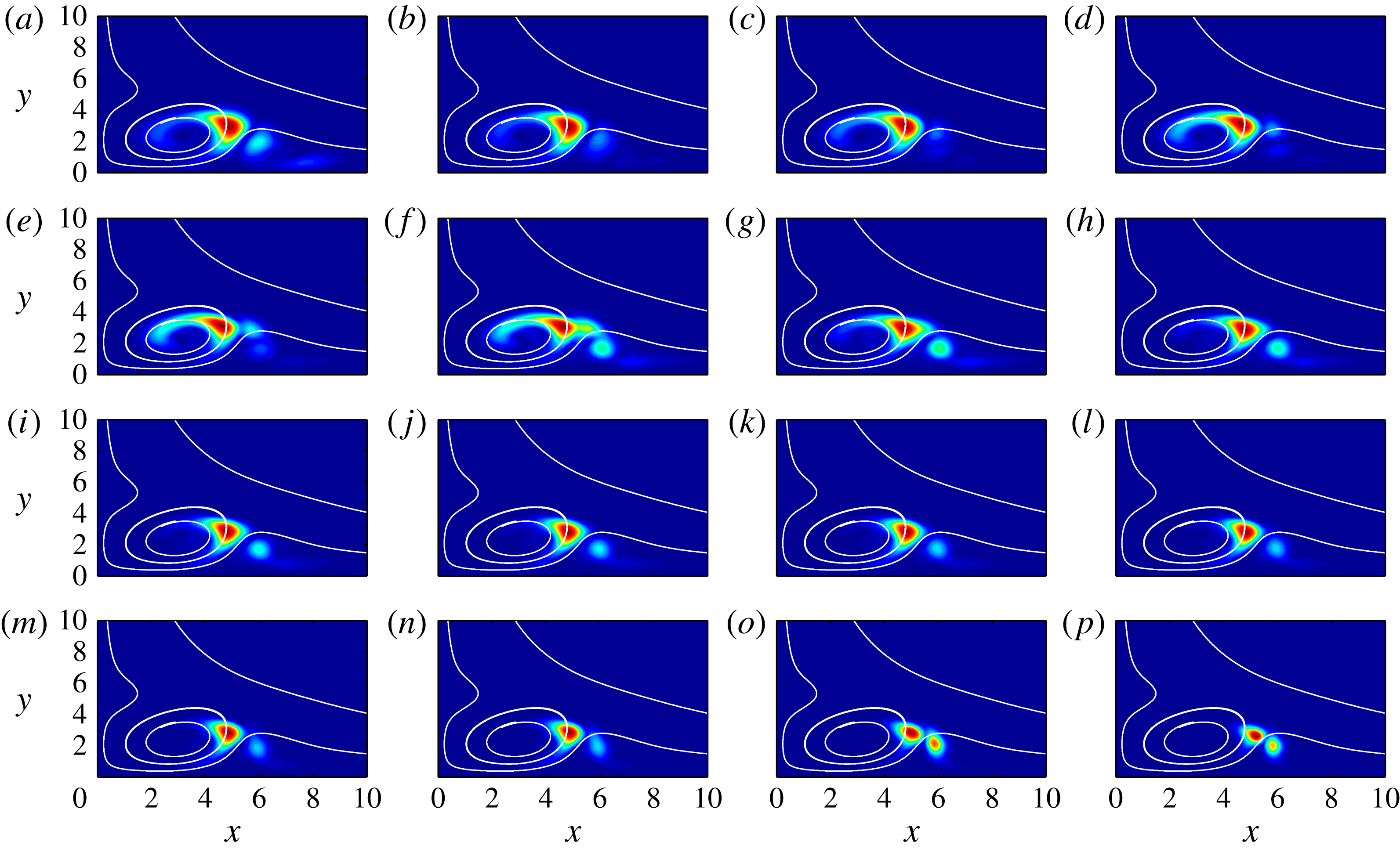
A typical dependence of branch
 $C$
eigenmodes on
 ${\it\gamma}$
is illustrated in figure 7. The eigenmode shape remains similar for different values of
 ${\it\gamma}$
and the maximum amplitude moves only slightly between the outside of the vortex and the upper shear layer. However, there are other modes which are more sensitive with respect to
 ${\it\gamma}$
and whose shape changes significantly as
 ${\it\gamma}$
is altered. Branch
 $G$
mode moves from the upper shear layer into the vortex and branch
 $F$
mode moves from the upper shear layer through the vortex towards the wall as
 ${\it\gamma}$
is increased.
3.4.2 Secondary neutral curve and marginally stable modes
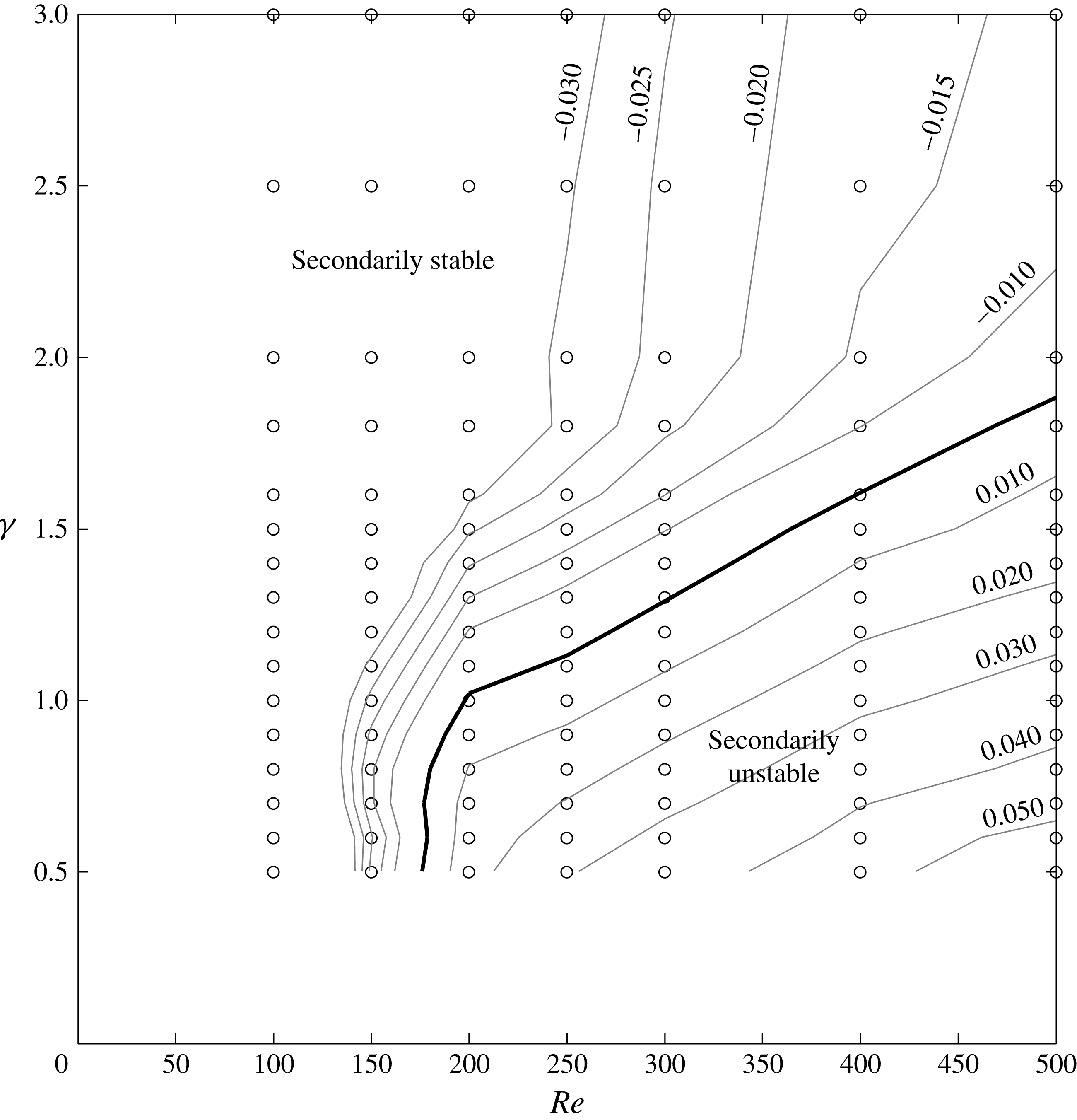
The spectra and results illustrated in figure 4(b) may be reduced to one secondary stability diagram, shown in figure 8. The typical shape of an upper branch of a neutral curve can be observed with a minimum (secondary critical) Reynolds number
 $Re_{sec,crit}\approx 175$
, wavenumber
 ${\it\gamma}_{sec,crit}\approx 0.5\ldots 0.7$
and phase speed
 $c_{r,sec,crit}\approx 0.86$
. For all investigated Reynolds numbers, the most amplified mode belongs to the
 $G$
branch (cf. figure 4
b). The magnitudes of its streamwise velocity components,
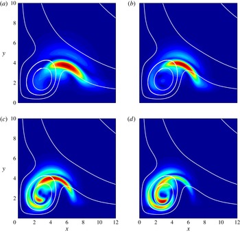
 $|\hat{\boldsymbol{v}}(x,y)|$
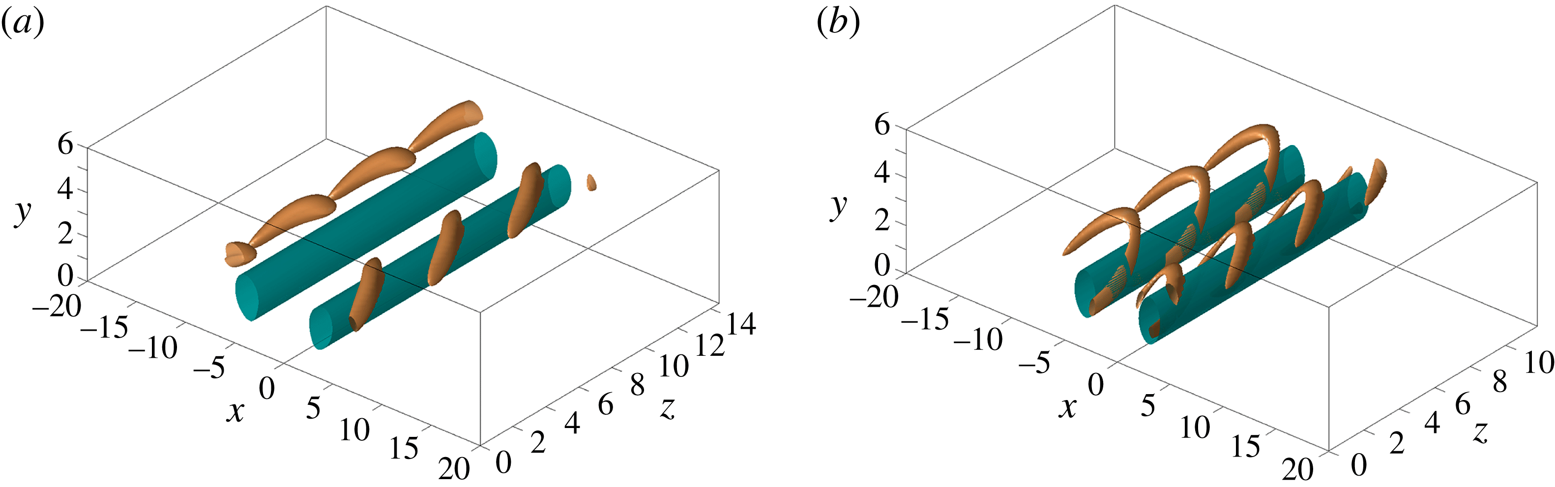
, are illustrated in figure 9 for four different points along the neutral curve. Their three-dimensional shape is illustrated in figure 10 for two different Reynolds numbers by isosurfaces of the
 ${\it\lambda}_{2}$
vortex criterion (Jeong & Hussain Reference Jeong and Hussain1995). The stability diagram only shows results for
 ${\it\gamma}\geqslant 0.5$
because the numerical solution to eigenvalue problem (3.3) starts to converge slowly when
 ${\it\gamma}$
is decreased towards
 ${\it\gamma}\approx 0.5$
, due to the slow spatial decay rates
 $\exp (-{\it\gamma}x_{i})$
in the
 $x$
and
 $y$
directions, which require an increasingly large computational domain.
Secondary stability diagram of the SHBL secondary baseflow as defined in § 2 without wall suction. The lines show contours of the temporal growth rate
 $c_{i}$
of the most amplified (or least damped) mode (values are indicated). The thick line is the neutral curve
 $c_{i}=0$
. Secondary instability is observed for Reynolds numbers
 $Re$
as low as
 $175$
. The open circles illustrate the parameter combinations
 $\{Re,{\it\gamma}\}$
for which stability equations (3.3) were solved.

Marginally stable secondary eigenmode of branch
 $G$
at (a)
 $Re=200$
,
 ${\it\gamma}=1.0$
(b)
 $Re=300$
,
 ${\it\gamma}=1.3$
(c)
 $Re=400$
,
 ${\it\gamma}=1.5$
(d)
 $Re=500$
,
 ${\it\gamma}=1.8$
.

Vortex of the baseflow
 $\boldsymbol{u}_{B}$
(turquoise) and a superposition of the baseflow and the antisymmetric secondary
 $G$
mode (gold) illustrated by
 ${\it\lambda}_{2}$
vortex structures,
 ${\it\lambda}_{2}=-0.02$
. (a)
 $Re=200$
,
 ${\it\gamma}=1.3$
and (b)
 $Re=400$
,
 ${\it\gamma}=1.6$
. Secondary disturbance velocity maximum
 $A_{2}=0.1$
.

3.4.3 Stabilization by suction
We investigate whether a stabilizing behaviour of homogeneous wall suction (
 ${\it\kappa}>0$
) is present for the secondary baseflow
 $\boldsymbol{u}_{B}$
. The streamwise baseflow velocity component
 $\boldsymbol{w}_{B}(x,y)$
increases by approximately
 $0.1W_{\infty }$
near the wall where the amplified modes have significant amplitude, leading to increased phase speeds
 $c_{r}$
of all modes. Furthermore, the growth rates
 $c_{i}$
of most of the discrete modes decrease with increasing suction (John et al.
Reference John, Obrist and Kleiser2014b
), analogously to the linear primary stability of the SHBL (Hall et al.
Reference Hall, Malik and Poll1984).
3.4.4 Quasi-degenerate eigenmodes
The results reported in the preceding subsections were obtained with boundary conditions (3.5c
) enforcing antisymmetric (
 $a$
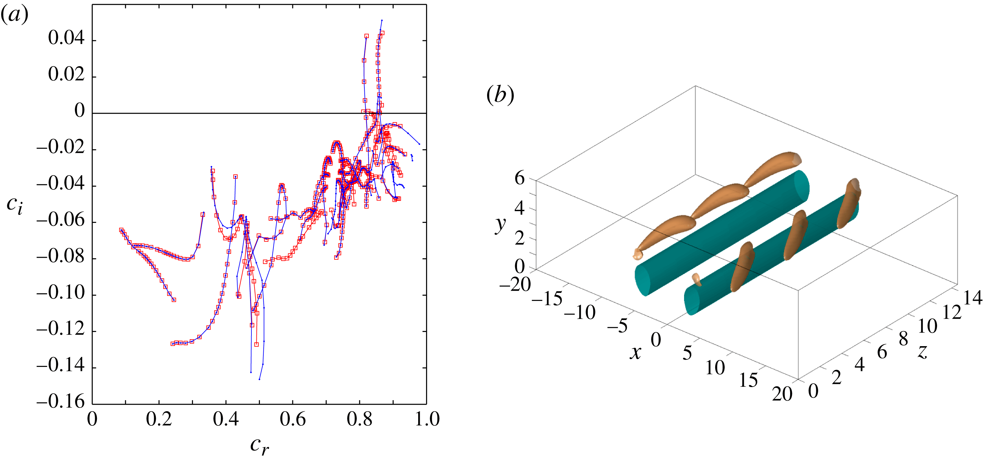
) modes. Surprisingly, the eigenvalues of the nine branches
 $A$
–
 $I$
highlighted in figure 4(b) are also observed for symmetric (
 $s$
) boundary conditions (3.5c
). Except for one purely antisymmetric branch located near
 $c_{r}\approx 0.83$
, the eigenvalues are almost identical. A comparison of the two spectra is illustrated in figure 11(a) for
 $Re=400$
. In general, we observe that the symmetric and antisymmetric eigenvalues are almost indistinguishable for large wavenumbers
 ${\it\gamma}$
, but that the branches start to diverge around
 ${\it\gamma}\approx 0.5$
(e.g. branches
 $A$
,
 $G$
and
 $H$
).
(a) Branches of symmetric modes (blue dots) and antisymmetric modes (red squares) for
 $Re=400$
,
 ${\it\gamma}\in [0.5,5.0]$
,
 ${\it\kappa}=0$
. (b) Vortex of the baseflow
 $\boldsymbol{u}_{B}$
(turquoise) and a superposition of the baseflow and the symmetric secondary
 $G$
mode (gold) illustrated by
 ${\it\lambda}_{2}$
vortex structures,
 $Re=200$
,
 ${\it\gamma}=1.3$
. Secondary disturbance amplitude
 $A_{2}=0.1$
,
 ${\it\lambda}_{2}=-0.02$
.

Despite the similarity of the symmetric and the antisymmetric eigenvalues illustrated in figure 11(a), the corresponding eigenmodes have opposite symmetry properties. The differences between these modes, however, are confined to a narrow layer near
 $x\approx 0$
where the symmetry boundary conditions (3.5c
) are satisfied. Inside the domain, away from this thin layer, the eigenmodes are nearly identical. Three-dimensional illustrations of the symmetric and antisymmetric
 $G$
eigenmodes are shown in figures 11(b) and 10(a). The figures unveil nearly indistinguishable mode shapes, but a clear phase difference between the individual vortex elements in the positive and negative chordwise domain halves.
Within the present numerical accuracy of four to five significant digits, it cannot be conclusively stated whether the eigenvalues are exactly degenerate or differ from each other slightly. However, we make reference to a similar phenomenon reported by Orszag (Reference Orszag1971) for the primary linear stability of plane Poiseuille flow (solution of the Orr–Sommerfeld equation). There, numerous symmetric and antisymmetric modes have eigenvalues which differ only after several significant digits, but which are distinct and not exactly degenerate. Possibly, the same phenomenon occurs for the secondary instability of the perturbed SHBL.
4 Direct numerical simulations of spatial instability and transition
In this section, we report results of direct numerical simulations (DNS) of the secondary baseflow
 $\boldsymbol{u}_{B}$
with a superimposed secondary, time-dependent disturbance. These simulations will validate the stability results from the preceding section and exhibit a bypass transition mechanism at subcritical Reynolds numbers
 $Re<Re_{crit}$
.
4.1 Time-dependent secondary disturbance
The DNS of spatial secondary instability require an additional secondary, time dependent, three-dimensional disturbance
 $\boldsymbol{u}_{2}^{\prime }$
of the secondary baseflow
 $\boldsymbol{u}_{B}$
introduced in § 2. Following Obrist et al. (Reference Obrist, Henniger and Kleiser2012),
 $\boldsymbol{u}_{2}^{\prime }$
is introduced as an oscillation of small amplitude
 $A_{2}^{\pm }$
superimposed onto the primary disturbance
 $\boldsymbol{u}_{1}^{\prime }$
of mean amplitude
 $A_{1}$
(2.1) at the secondary disturbance frequency
 ${\it\omega}_{2}=2{\rm\pi}/T_{2}$
. The amplitude of this secondary disturbance is approximately
 $A_{2}^{\pm }/A_{1}\approx 10^{-3}$
. The total disturbance
 $\boldsymbol{u}^{\prime }=\boldsymbol{u}_{1}^{\prime }+\boldsymbol{u}_{2}^{\prime }=\boldsymbol{u}-\boldsymbol{u}_{SH}$
thus reads
 $$\begin{eqnarray}\boldsymbol{u}^{\prime }(x,y,t)|_{z=0}=\boldsymbol{u}_{1}^{\prime }(x,y)[1+\underbrace{A_{2}^{\pm }\sin ({\it\omega}_{2}t)}_{\text{sec. dist.}}].\end{eqnarray}$$
 $A_{2}^{-}$
is the amplitude of the secondary oscillation of the primary vortex located in the negative chordwise domain
 $x<0$
and
 $A_{2}^{+}$
that of the vortex located in the domain of positive
 $x$
. The oscillation may either be synchronous (symmetric secondary disturbance,
 $A_{2}^{-}=A_{2}^{+}$
), or it may have a
 $180^{\circ }$
phase shift (antisymmetric,
 $A_{2}^{-}=-A_{2}^{+}$
).
4.2 Numerical simulation method
The DNS are carried out with our in-house Navier–Stokes solver IMPACT which is described in detail by Henniger, Obrist & Kleiser (Reference Henniger, Obrist and Kleiser2010) and Henniger (Reference Henniger2011). The NSE are discretized in all three spatial directions by sixth-order finite differences on a stretched Cartesian grid. Explicit time integration is performed for the present simulations (third-order Runge–Kutta integration), but the results and run time do not differ significantly when employing a semi-implicit integration. A typical computational domain size is
 $L_{x}\times L_{y}\times L_{z}=75\times 30\times 600$
discretized with
 $N_{x}\times N_{y}\times N_{z}\approx 750\times 150\times 3000$
grid points. The code allows for solving the NSE in parallel with excellent weak and strong scaling properties by using domain block decomposition in all three directions. The pressure equation is solved in parallel at every integration substep with a preconditioned multigrid algorithm.
The implementation of the disturbances and the boundary conditions follow Obrist et al. (Reference Obrist, Henniger and Kleiser2012) and John et al. (Reference John, Obrist and Kleiser2014b
). The computational domain has inflow planes at
 $z=0$
and
 $y=L_{y}$
and one (optionally permeable) wall at
 $y=0$
. At the inflow plane
 $z=0$
, the SHBL
 $\boldsymbol{u}_{SH}$
and the primary and secondary disturbances
 $\boldsymbol{u}_{1}^{\prime }$
and
 $\boldsymbol{u}_{2}^{\prime }$
are prescribed as Dirichlet conditions. The undisturbed SHBL
 $\boldsymbol{u}_{SH}$
is prescribed by Dirichlet conditions at
 $y=0,L_{y}$
.
The flow leaves the domain at the three remaining outflow planes
 $x=\pm L_{x}$
and
 $z=L_{z}$
. There, an advective boundary condition is imposed for the velocity disturbances
 $\boldsymbol{u}^{\prime }=\boldsymbol{u}-\boldsymbol{u}_{SH}$
. For the outward-normal direction
 $x_{n}$
the boundary conditions read
 $\partial \boldsymbol{u}^{\prime }/\partial t+C\partial \boldsymbol{u}^{\prime }/\partial x_{n}=\mathbf{0}$
, where
 $C$
is a constant convection velocity, set to 1.5 times the maximum wall-normal SHBL velocity component on that outflow plane (John Reference John2014).
4.3 Fourier–Hermite spectral analysis
We quantitatively analyse the secondary instability by employing a Fourier–Hermite spectral decomposition of the instantaneous disturbance flow field
 $\boldsymbol{u}^{\prime }=\boldsymbol{u}-\boldsymbol{u}_{SH}$
following Obrist & Schmid (Reference Obrist and Schmid2003a
). The analysis provides the time-independent spectral disturbance energy densities
 $$\begin{eqnarray}\displaystyle & \displaystyle e_{k,n}(z)=\int _{0}^{\infty }(|\tilde{\boldsymbol{u}}_{k,n}^{\prime }|^{2}+|\tilde{\boldsymbol{v}}_{k,n-1}^{\prime }|^{2}+|\tilde{\boldsymbol{w}}_{k,n-1}^{\prime }|^{2})\,\text{d}y, & \displaystyle\end{eqnarray}$$
 $$\begin{eqnarray}\displaystyle & \displaystyle \text{with}~\tilde{\boldsymbol{u}}_{k,n}^{\prime }=\int _{t_{a}}^{t_{b}}\int _{-\infty }^{\infty }\boldsymbol{u}^{\prime }(x,y,z,t)He_{n}(x)\text{e}^{-(x/(\sqrt{2}{\it\tau}))^{2}}\,\text{d}x\text{e}^{-\text{i}k{\it\omega}_{2}t}\,\text{d}t. & \displaystyle\end{eqnarray}$$
 $n$
stands for the order of the chordwise Hermite polynomials
 $\mathit{He}_{n}(x)$
and
 $k$
for the temporal (Fourier) harmonic. A typical parameter of the Gaussian weight function is
 ${\it\tau}=10$
(Obrist & Schmid Reference Obrist and Schmid2003b
). We initiate the analysis at some time
 $t_{a}$
when the simulations have attained a statistically stationary state and the integration interval
 $t_{b}-t_{a}$
contains a sufficiently large number of secondary disturbance periods
 $T_{2}=2{\rm\pi}/{\it\omega}_{2}$
(at least 15). The energy densities
 $e_{k,n}$
(4.2) are useful quantities for the analysis of the secondary instability downstream of the development of the VSS.
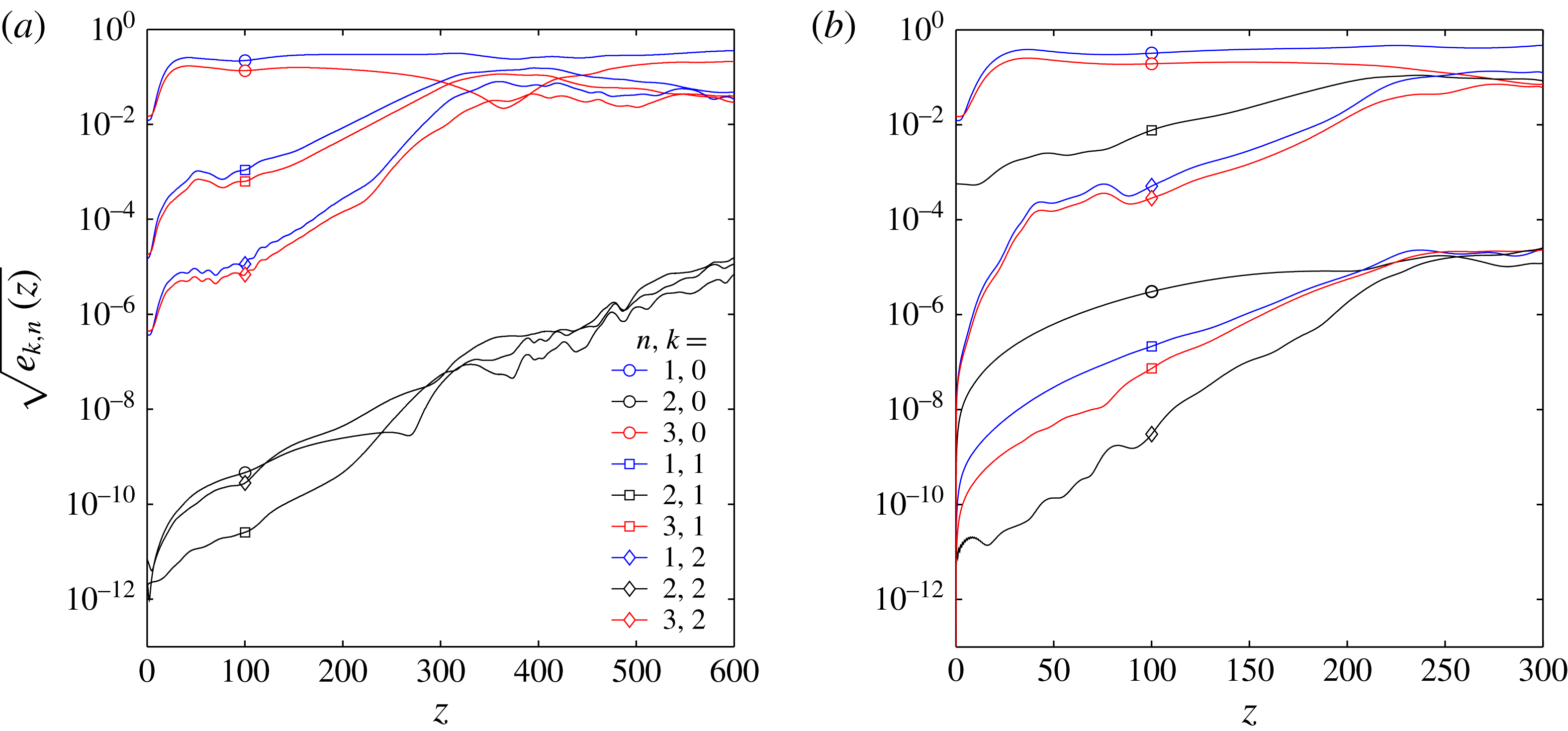
Typical Fourier–Hermite spectral energy densities
 $e_{k,n}(z)$
for (a) a symmetric secondary disturbance,
 ${\it\kappa}=0.6$
,
 ${\it\omega}_{2}\approx 0.21$
, (b) an antisymmetric secondary disturbance,
 ${\it\kappa}=0$
,
 ${\it\omega}_{2}\approx 0.16$
.
 $Re=370$
,
 $A_{1}=0.1$
.

4.4 Results
4.4.1 Secondary instability
Typical evolutions of
 $e_{k,n}$
for unstable flows are shown in figure 12. Panel (a) illustrates results for a symmetric secondary perturbation, (b) for an antisymmetric one. In both cases the VSS, which is stationary (
 $k=0$
) and symmetric (
 $n$
odd), contains almost all the energy at the inflow plane
 $z=0$
(blue and red circles). Very little energy is contained in the secondary perturbation (
 $k=1$
,
 $n$
odd in (a) and
 $n$
even in (b)). The remaining modes contain no energy other than numerical noise due to discretization errors and floating-point arithmetic. Far downstream, however, these modes grow to substantial values along with the breakdown to turbulent flow. A secondary spatial modal instability can be observed after a short initial interval within which the steady primary VSS (
 $k=0$
) obtains its energy due to non-modal growth (
 $0<z\lessapprox 2z_{max}$
). The exponential energy growth rate
 ${\it\beta}$
is obtained from the slope of the energy density which corresponds to the secondary instability mode at some suitable location
 $z^{\ast }$
which marks the onset of secondary modal growth (e.g.
 $z^{\ast }\approx 120$
in figure 12(a) or
 $z^{\ast }\approx 80$
in (b)). The relevant energy density
 $e_{k,n}$
is the first harmonic (
 $k=1$
) and either the first-order chordwise polynomial (
 $n=1$
, for symmetric secondary disturbances, blue square), or the second-order chordwise polynomial (
 $n=2$
, for antisymmetric disturbances, black square), i.e.
 $$\begin{eqnarray}\text{either}\quad e_{1,1}(z)\approx e_{1,1}(z=z^{\ast })\text{e}^{{\it\beta}(z-z^{\ast })}~(s)\quad \text{or}\quad e_{1,2}(z)\approx e_{1,2}(z=z^{\ast })\text{e}^{{\it\beta}(z-z^{\ast })}~(a).\end{eqnarray}$$
Typically, at least one such location
 $z^{\ast }$
is present. Depending on the secondary disturbance frequency
 ${\it\omega}_{2}$
, even two locations may be identified, suggesting the presence of two distinct secondary modes with different growth rates.
Simulations with identical baseflows
 $\boldsymbol{u}_{B}$
(
 $Re=300$
,
 ${\it\kappa}=0.4$
,
 $A_{1}=0.1$
) disturbed at secondary disturbance frequencies (a)
 ${\it\omega}_{2}\approx 0.63$
, (b)
 ${\it\omega}_{2}\approx 0.31$
, (c)
 ${\it\omega}_{2}\approx 0.21$
.
 ${\it\lambda}_{2}$
isosurfaces of the instantaneous flow
 $\boldsymbol{u}$
.

Spatial energy growth rates
 ${\it\beta}$
of (a) antisymmetric secondary instability mode
 $e_{1,2}$
and (b) symmetric secondary instability mode
 $e_{1,1}$
as functions of
 ${\it\omega}_{2}$
.
 $Re=370$
,
 ${\it\kappa}=0$
,
 $A_{1}=0.1$
. The dotted curve in (b) illustrates the growth rate
 ${\it\beta}^{G}$
estimated by Gaster’s transformation (4.4).

4.4.2 Frequency dependence
The secondary energy growth rate
 ${\it\beta}$
, defined according to (4.3), depends strongly on the secondary disturbance frequency
 ${\it\omega}_{2}$
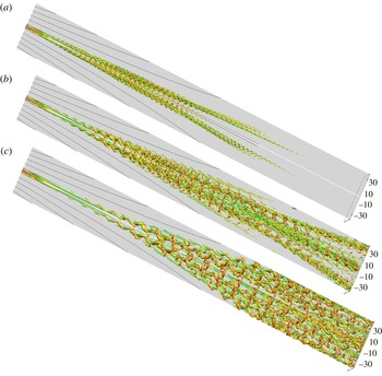
. Figure 13 illustrates this by three visualizations of
 ${\it\lambda}_{2}$
isosurfaces for identical baseflows
 $\boldsymbol{u}_{B}$
but different disturbance frequencies
 ${\it\omega}_{2}$
. The energy growth rates
 ${\it\beta}$
increase from (a) to (c), resulting in ever larger regions contaminated by high-amplitude disturbances. In (a), the secondary growth is so weak that there is no breakdown to turbulent flow and the perturbations vanish far downstream. In (c), on the other hand, the boundary layer becomes turbulent.
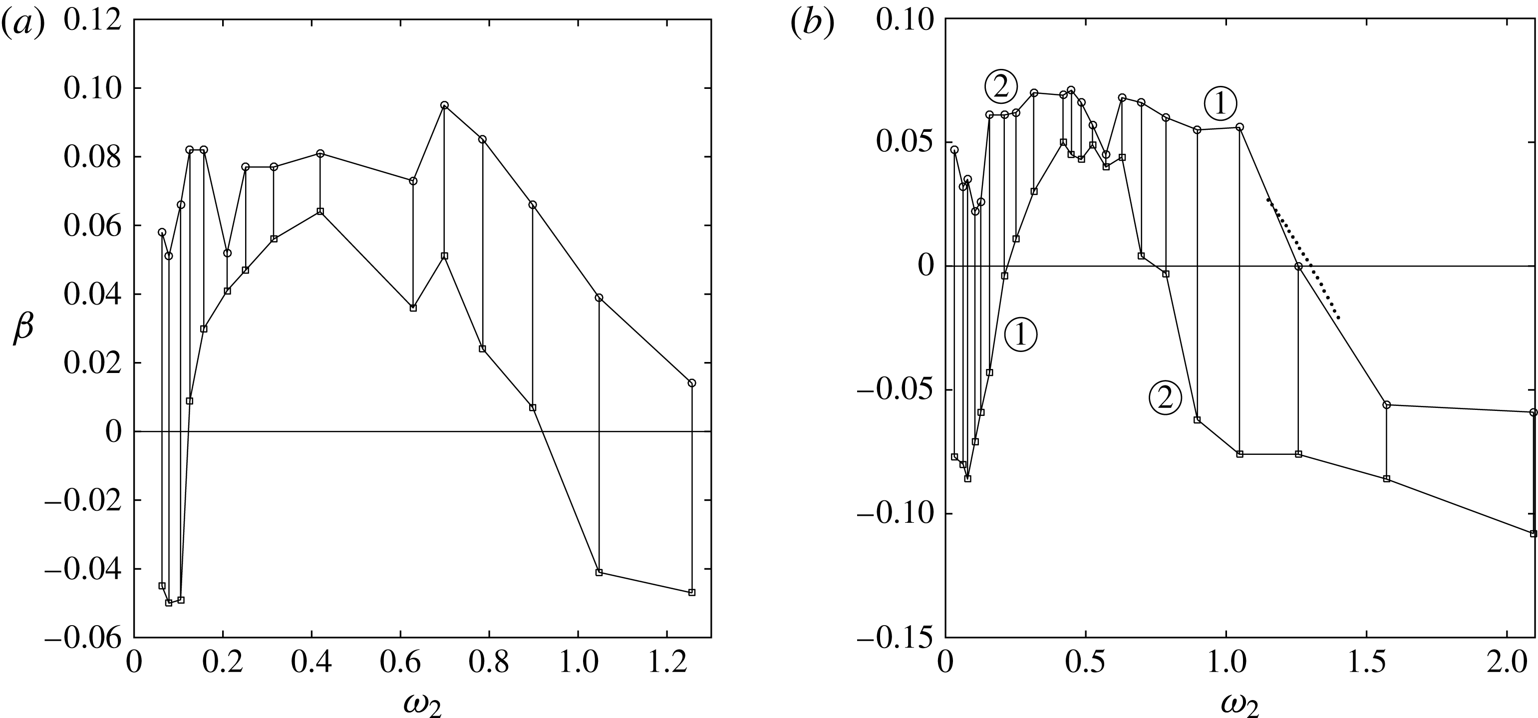
Quantitative results are shown in figure 14, which illustrates
 ${\it\beta}({\it\omega}_{2})$
both for symmetric and for antisymmetric secondary disturbances. The determination of a single precise value
 ${\it\beta}$
from
 $e_{k,n}$
can be ambiguous (cf. figure 12) due to the sensitivity with respect to
 $z^{\ast }$
(cf. (4.3)). Therefore, we determine two growth rates
 $\{{\it\beta}_{max},{\it\beta}_{min}\}$
for each simulation. They mark the respective upper and lower bound for sensible estimates of
 ${\it\beta}$
. Interestingly, for a wide range of frequencies
 ${\it\omega}_{2}$
two distinct regions of exponential growth can be observed at disjoint
 $z$
intervals. This indicates the existence of two different eigenmodes which both grow exponentially, but at different rates. The two curves marked by
 $\unicode[STIX]{x2460}$
and
 $\unicode[STIX]{x2461}$
in figure 14(b) therefore represent two independent secondary modes. Mode
 $1$
is growing faster than mode
 $2$
at high frequencies and vice versa at low frequencies. Their energy growth rates
 ${\it\beta}({\it\omega}_{2})$
are roughly equal at
 ${\it\omega}_{2}\approx 0.6$
. For antisymmetric disturbances (figure 14
a), the picture is less obvious: the maximum and minimum growth rates are slightly closer to each other than in the symmetric case, and the
 $z$
intervals of exponential growth are not that clearly separated. We cannot conclusively state whether the two curves describe the evolution of two independent modes, or whether they emerge from a rather noisy exponential growth of one amplified secondary eigenmode. Altogether, the symmetric and antisymmetric disturbances illustrated in figure 14(a,b) exhibit very similar growth rates. This is consistent with results of § 3.4.4 where it was demonstrated that the secondary symmetric and antisymmetric eigenmodes are quasi-degenerate.
4.4.3 Validation of secondary stability results
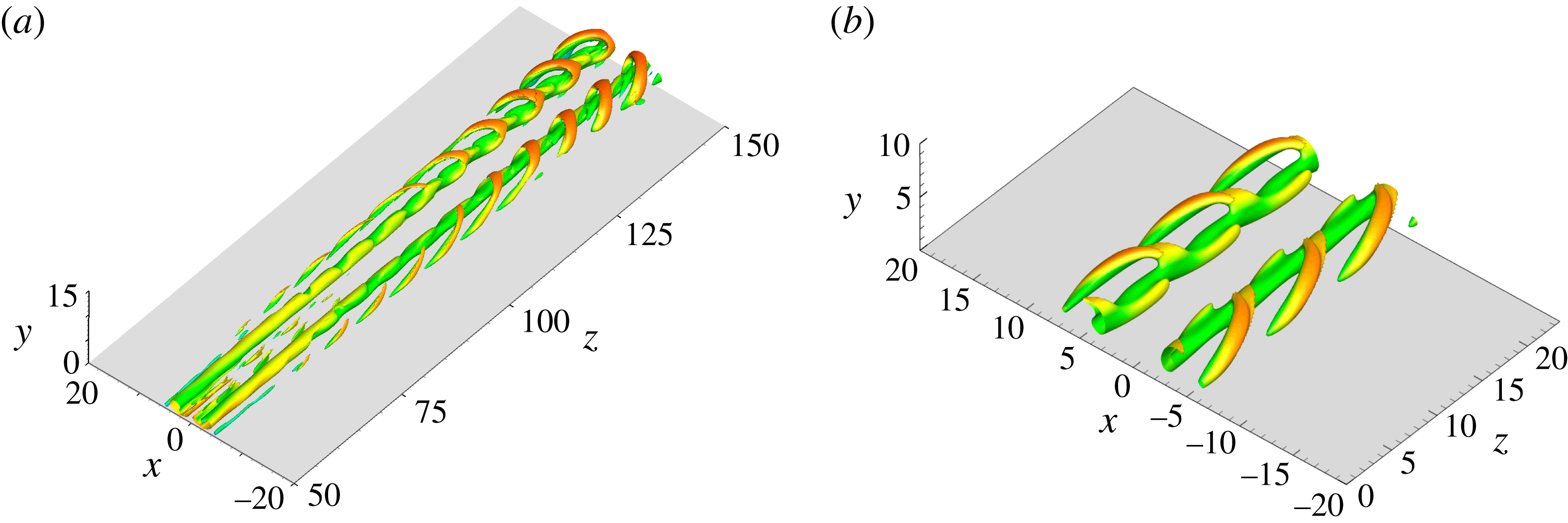
We compare the spatial secondary instability results obtained in DNS with those from SSA of § 3, first qualitatively and then quantitatively. Figure 15(a) illustrates
 ${\it\lambda}_{2}$
isosurfaces of the total DNS flow field
 $\boldsymbol{u}$
for
 $Re=370,{\it\kappa}=0$
, coloured according to the local streamwise velocity
 $w$
. For this parameter combination, the quasi-periodic secondary vortices have a spatial wavelength
 $2{\rm\pi}/{\it\gamma}^{DNS}\approx 8$
for a large streamwise extent. We compare them to the secondary eigenmodes obtained from temporal stability analysis for
 ${\it\gamma}=0.8$
at the parameter combination
 $Re=400,{\it\kappa}=0$
, illustrated in figure 15(b) using an arbitrary mode amplitude. Near
 $z=100$
, where the baseflow
 $\boldsymbol{u}_{B}$
was extracted for stability analysis, the secondary modes observed in the DNS look qualitatively very similar to those obtained from SSA.
(a) Secondary vortical structures from DNS, illustrated by the
 ${\it\lambda}_{2}$
vortex criterion applied to the full velocity field (
 ${\it\lambda}_{2}=-10^{-4}$
),
 $Re=370$
,
 ${\it\kappa}=0$
,
 $A_{1}=0.10$
,
 ${\it\omega}_{2}\approx 0.63$
. (b) Secondary eigenmodes from SSA, illustrated for three periods by the
 ${\it\lambda}_{2}$
vortex criterion applied to the full velocity field (amplitude of secondary disturbances
 $A_{2}=0.09$
,
 ${\it\lambda}_{2}=-2\times 10^{-3}$
),
 $Re=400$
,
 ${\it\kappa}=0$
,
 ${\it\gamma}=0.8$
. Isosurfaces in both figures are coloured according to the local streamwise velocity component
 $w(x,y,z,t)$
(red: high velocity; green: low velocity).

We carry out two quantitative comparisons of the DNS and SSA results. First, we compare the respective neutral curves, then we apply Gaster’s transformation to compare growth rates. The DNS exhibit marginal secondary stability for a symmetric secondary disturbance with parameters
 $\{Re,{\it\omega}_{2}\}=\{370,1.257\}$
(cf. figure 14
b). The spatial wavenumber of the secondary vortices observed in that DNS is found to be
 ${\it\gamma}^{DNS}\approx 1.5$
. This is in good agreement with the neutral curve of the temporal SSA, which predicts a critical wavenumber
 ${\it\gamma}_{c}\approx 1.515$
at
 $Re=370$
(see figure 8). The phase velocity
 $c_{r}^{DNS}$
of the mode observed in the DNS follows from
 $c_{r}^{DNS}={\it\omega}_{2}/{\it\gamma}^{DNS}\approx 1.26/1.5\approx 0.84$
. This value is in good agreement with the phase velocity
 $c_{r,c}\approx 0.859$
of the neutrally stable
 $G$
mode obtained from SSA (see figure 4
b). In summary, both the spatial wavenumber
 ${\it\gamma}$
and the phase velocity
 $c_{r}$
of the marginally stable symmetric mode (growth rates
 $c_{i}={\it\beta}=0$
) are nearly equal in the spatial DNS and the temporal SSA for
 $Re=370$
.
In addition to this comparison on the neutral curve, we can compare the spatial secondary energy growth rates
 ${\it\beta}$
obtained in our DNS to results from our temporal SSA in the vicinity of the neutral curve by carrying out Gaster’s transformation (Gaster Reference Gaster1962). For
 $Re=370$
, the neutral curve is found at
 ${\it\gamma}\approx 1.515$
(see figure 8). At this point we determine the group velocity from our SSA results,
 $\partial {\it\omega}_{r}/\partial {\it\gamma}\approx 0.8747$
. We can approximate the temporal growth rate
 ${\it\omega}_{i}$
of the SSA by the second-order polynomial
 ${\it\omega}_{i}({\it\omega}_{r})\approx p_{1}{\it\omega}_{r}^{2}+p_{2}{\it\omega}_{r}+p_{3}$
with
 $p_{1}=-0.05409$
,
 $p_{2}=0.05503$
,
 $p_{3}=0.01992$
. According to Gaster’s transformation, this allows us to calculate an estimate of the spatial growth rates
 $-{\it\gamma}_{i}^{G}({\it\omega}_{r})$
near the neutral curve according to
 $$\begin{eqnarray}-{\it\gamma}_{i}^{G}({\it\omega}_{r})=\frac{{\it\omega}_{i}({\it\omega}_{r})}{\partial {\it\omega}_{r}/\partial {\it\gamma}}.\end{eqnarray}$$
This estimate may be compared to half of the negative energy growth rates obtained from our DNS (4.3),
 ${\it\beta}\approx -2{\it\gamma}_{i}^{G}({\it\omega}_{r})$
. The comparison is illustrated in figure 14 by a dotted line. Again, the results from SSA and DNS are in excellent agreement.
These qualitative and quantitative comparisons demonstrate that the SSA and the three-dimensional DNS results exhibit the same secondary instability.
4.4.4 Comparison of DNS results to experiments and simulations from the literature
Finally, we compare our transition results obtained by DNS with those from experiments and simulations reported in the literature. To this end we analyse the transition Reynolds number
 $Re_{tr}$
at which turbulent flow can first be observed and its dependence on the wall suction strength
 ${\it\kappa}$
. It is known that wall suction (
 ${\it\kappa}>0$
) stabilizes the attachment-line flow both by extending the region of primary linear stability (Hall et al.
Reference Hall, Malik and Poll1984; Joslin Reference Joslin1995) and by inhibiting the transition to turbulence (Spalart Reference Spalart1988; Poll & Danks Reference Poll and Danks1995; Arnal et al.
Reference Arnal, Juillen, Reneaux and Gasparian1997).
We call a flow transitional if two criteria are met. First, those modal energies
 $e_{n,k}$
which obtain energy
 $e_{n,k}$
from nonlinear processes only (e.g.
 $n=2$
modes (black curves) in figure 12) must exhibit a monotonic growth trend or remain at quasi-saturation level until the domain boundary is reached. Second, we must be able to observe the breakdown of coherent vortex structures (cf. figure 13
c) from three-dimensional
 ${\it\lambda}_{2}$
vortex visualizations.
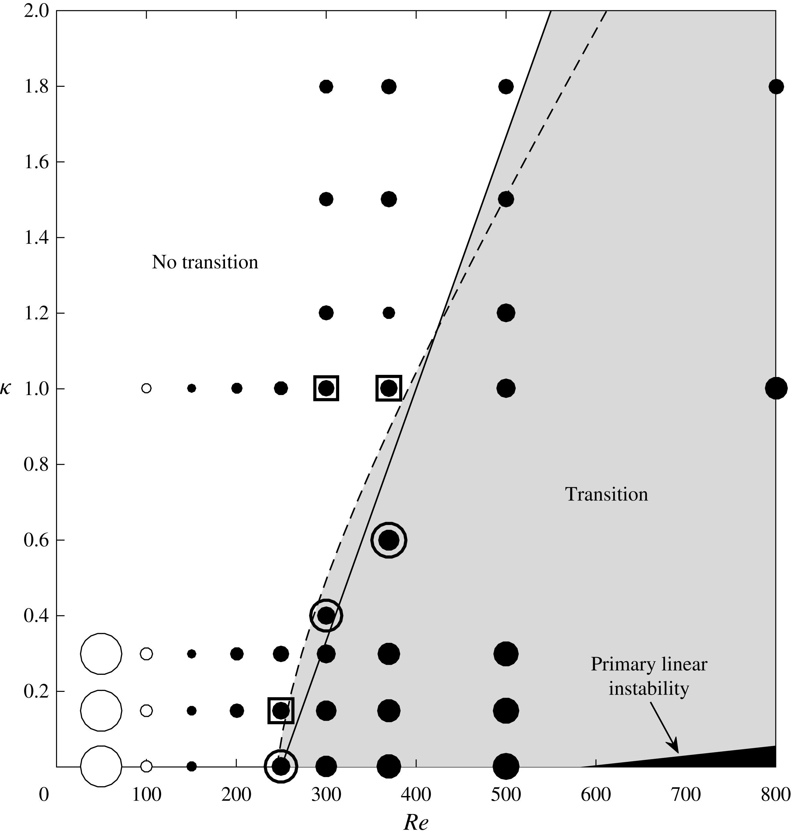
Figure 16 summarizes our findings for various
 $Re$
and
 ${\it\kappa}$
. It is important to emphasize again that our results are independent of the primary disturbance amplitude
 $A_{1}$
, as long as it is large enough to lead to quasi-saturation of
 $A_{st}$
(cf. § 2.2). The figure illustrates the secondary spatial growth rates (4.3) by the radii of filled (
 ${\it\beta}>0$
) and open (
 ${\it\beta}<0$
) circles. In the absence of suction, clearly positive growth rates
 ${\it\beta}>0$
are observed for
 $Re\geqslant 200$
. The growth rates for
 $Re\approx 150$
are nearly zero, and
 $Re=100$
is the largest Reynolds number at which
 ${\it\beta}$
is clearly negative. Figure 16 comprises three distinct regimes. First, for very low Reynolds numbers, the flows show secondary stability (
 ${\it\beta}<0$
), such that all secondary disturbances decay eventually, some of them after a short transient period. Second, for large Reynolds numbers, the flows are clearly unstable (
 ${\it\beta}>0$
) and undergo transition to turbulence. In the third regime, at intermediate Reynolds numbers
 $100\lessapprox Re\lessapprox 250$
for
 ${\it\kappa}=0$
, flows are secondarily unstable (
 ${\it\beta}>0$
), but do not break down to turbulent flow, but rather return to the laminar baseflow eventually. In this regime of weak modal growth, the secondary instability is not persistent and the VSS decays too quickly for the flow to become turbulent. In particular, this explains why the experimentally known transition boundaries
 $Re_{tr}({\it\kappa})$
do not coincide with the neutral curve
 $c_{i}=0$
of the secondary instability (cf. figures 8 and 16).
Spatial energy growth rates
 ${\it\beta}$
(4.3) of the secondary symmetric mode
 $e_{1,1}$
as a function of
 $Re$
and wall suction strength
 ${\it\kappa}$
for
 $A_{1}=0.1$
,
 ${\it\omega}_{2}\approx 0.21$
. Filled circles denote positive, open circles negative growth rates
 ${\it\beta}$
, their radii indicate the magnitude of
 ${\it\beta}$
(not to scale). The solid curve (Arnal et al.
Reference Arnal, Juillen, Reneaux and Gasparian1997) and the dashed curve (Poll & Danks Reference Poll and Danks1995) show experimental results for the transition Reynolds number
 $Re_{tr}({\it\kappa})$
. For comparison, six DNS for parameters close to these curves were tested for transition: the three DNS below the curve of Poll & Danks (Reference Poll and Danks1995) clearly showed transition to turbulent flow (circles), and three DNS above the curve showed return to laminar flow (squares). The small black area in the bottom right corner represents the region of primary linear instability.

In addition, figure 16 also illustrates two expressions for the transition Reynolds number as function of the wall suction strength
 $Re_{tr}({\it\kappa})$
known from the literature. These expressions for
 $Re_{tr}({\it\kappa})$
were determined from experiments by Danks & Poll (Reference Danks, Poll, Duck and Hall1995), Poll & Danks (Reference Poll and Danks1995) and Arnal et al. (Reference Arnal, Juillen, Reneaux and Gasparian1997), and from numerical simulations by Spalart (Reference Spalart1988), who studied turbulent flow by employing periodic boundary conditions in the sweep direction. Both expressions are in close agreement with each other, and predict flow transition in the area of the parameter space highlighted in grey. For comparison, we inspect our DNS results immediately above and below the curve of Poll & Danks (Reference Poll and Danks1995) for
 $Re\in \{250,300,350\}$
. Those DNS in the immediate vicinity of the experimental boundary for transition are highlighted in figure 16 by an extra circle if they undergo transition to turbulence, those which remain laminar by a square.
We find that our DNS results are in close agreement with the estimates for
 $Re_{tr}({\it\kappa})$
from the literature. In particular, transition is observed for the parameter combination
 $Re=250$
,
 ${\it\kappa}=0$
, as illustrated in figure 17. In contrast, flows with
 $Re,{\it\kappa}$
only slightly left of
 $Re_{tr}({\it\kappa})$
return to the laminar baseflow even when secondary instability (
 ${\it\beta}>0$
) is observed for a limited streamwise extent. Detailed three-dimensional vortical structures of five such simulations highlighted in figure 16 are presented in John (Reference John2014, pp. 151–152). Details on the stabilizing influence of wall suction are documented in John et al. (Reference John, Obrist and Kleiser2014b
).
Illustration of subcritical transitional flow (
 ${\it\lambda}_{2}$
vortices coloured by local streamwise
 $w$
velocity component) due to a symmetric secondary instability at
 $Re=250$
,
 ${\it\kappa}=0$
,
 $A_{1}=0.12$
,
 ${\it\omega}_{2}\approx 0.31$
,
 ${\it\lambda}_{2}=-10^{-4}$
.

5 Summary and conclusions
The present paper presents a numerical investigation of the subcritical instability and transition which is well known to occur in swept cylinder or swept-wing leading-edge boundary-layer flow with and without suction.
We carried out a secondary, biglobal, temporal stability analysis of the LEBL subject to a finite-amplitude primary disturbance, which is computed as a stationary Navier–Stokes solution. Furthermore, we presented DNS at subcritical Reynolds numbers
 $Re<Re_{crit}\approx 583.1$
. For both tasks, we used the SHBL along a flat plate with and without suction as a model for the LEBL. At the inflow plane, we superimposed primary disturbances onto this boundary layer, which consist in counter-rotating streamwise vortices of finite amplitude. By advection of shear, they lead to a pronounced high-speed streak along the attachment line.
The stability analysis of this flow revealed numerous discrete secondary eigenvalues and associated eigenmodes, some of which are amplified at Reynolds numbers as low as
 $Re=175$
, far below the linear critical value
 $Re_{crit}$
and also clearly below the experimentally reported transition Reynolds number
 $Re_{tr}\approx 250$
. Almost all eigenmodes appear in symmetric/antisymmetric pairs, i.e. they are quasi-degenerate eigenvalues with almost indistinguishable eigenmodes. The shapes of the eigenmodes resemble strongly those found in secondary cross-flow instability. As in primary stability analysis, wall suction also reduces the secondary instability growth rates of the flow.
In our three-dimensional DNS, we superimposed a weak secondary disturbance in the form of an oscillation of the primary disturbance at constant temporal frequency
 ${\it\omega}_{2}$
. We observed the same modal instability as predicted by the secondary stability analysis, with consistent growth rates and modal shapes. For a broad range of parameters, the flow underwent transition to turbulent flow as a consequence of this secondary instability. The lowest Reynolds number for which we observed transition at zero suction is
 $Re_{tr}=250$
, the value commonly accepted as the lower boundary for transition according to experiments and numerical investigations. We found that wall suction increases the transition Reynolds number
 $Re_{tr}$
, and the dependence of
 $Re_{tr}$
on wall suction was found to well match that of several experimental and numerical studies. This secondary instability and transition mechanism, which is based on a vortex–streak-shear configuration in a weakly non-parallel boundary layer, closely resembles the self-sustained instability process known from parallel flat-plate boundary layers.
We conclude that the LEBL may show a secondary modal instability when counter-rotating vortices are present near the attachment line. The subsequent transition mechanism exhibited in this paper is triggered by this secondary instability, and can quantitatively explain the subcritical transition observed in leading-edge boundary-layer flow. The connection of these results to relevant receptivity mechanisms, such as those listed in the introduction, might lead to a comprehensive theory for leading-edge transition.
Acknowledgements
We acknowledge the instructive comments of the second referee with respect to the receptivity mechanisms outlined in the introduction, and the support of this work by ETH Zurich (ETH Research grant 19 12-2) and the Swiss National Supercomputing Centre CSCS (project ID s391).
Appendix A
This appendix describes how the matrices
 $\unicode[STIX]{x1D64B}$
and
 $\unicode[STIX]{x1D64C}$
of the eigenvalue problem (3.6) are constructed. The five-point finite difference stencil coefficients
 $\boldsymbol{c}_{m}$
for a stretched grid are defined following Henniger et al. (Reference Henniger, Obrist and Kleiser2010). In order to find the
 $d$
th derivative in the
 $x$
-direction at every grid point
 $x=x_{j},j=1,\ldots ,N_{x}$
, we define the square matrix
 $\unicode[STIX]{x1D63C}$
,
 $$\begin{eqnarray}\unicode[STIX]{x1D63C}=a_{nm}={\rm\Delta}x_{n}^{m-1},\quad n,m=1,\ldots ,5,\end{eqnarray}$$
where
 ${\rm\Delta}x_{n}=x_{j}-x_{n}$
. The stencil coefficient row vector
 $\boldsymbol{c}_{m}$
is obtained as the
 $(1+d)$
th row of the transpose inverse transpose of
 $\unicode[STIX]{x1D63C}$
,
 $$\begin{eqnarray}\boldsymbol{c}_{m}=d![\unicode[STIX]{x1D63C}^{-\text{T}}]_{(1+d),m}^{\text{T}}.\end{eqnarray}$$
The differentiation stencil is central within the domain and becomes one sided at the boundary points
 $j=\{1,N_{x}\}$
and partly one sided at the grid points
 $j=\{2,N_{x-1}\}$
adjacent to the boundary. The stencils are stored in band matrices
 ${\bf\delta}^{x},{\bf\delta}^{xx}\in \mathbb{R}^{N_{x}\times N_{x}}$
for the first and second derivatives in the
 $x$
-direction, respectively. Analogously, we obtain
 ${\bf\delta}^{y},{\bf\delta}^{yy}\in \mathbb{R}^{N_{y}\times N_{y}}$
for the first and second derivatives in the
 $y$
-direction. The differentiation matrices
 $\{\unicode[STIX]{x1D60B}_{x},\unicode[STIX]{x1D60B}_{xx},\unicode[STIX]{x1D60B}_{y},\unicode[STIX]{x1D60B}_{yy}\}\in \mathbb{R}^{N_{x}N_{y}\times N_{x}N_{y}}$
for the entire field, which may be applied to the velocity vectors of size
 $\mathbb{C}^{N_{x}Ny}$
, are obtained from tensor products with identity matrices
 $\unicode[STIX]{x1D610}_{N_{x}}\in \mathbb{N}^{N_{x}\times N_{x}}$
,
 $\unicode[STIX]{x1D610}_{N_{y}}\in \mathbb{N}^{N_{y}\times N_{y}}$
, respectively,
 $$\begin{eqnarray}\displaystyle \unicode[STIX]{x1D60B}_{x}=\unicode[STIX]{x1D610}_{N_{y}}\otimes {\bf\delta}^{x}\quad \unicode[STIX]{x1D60B}_{xx}=\unicode[STIX]{x1D610}_{N_{y}}\otimes {\bf\delta}^{xx} & & \displaystyle\end{eqnarray}$$
 $$\begin{eqnarray}\displaystyle \unicode[STIX]{x1D60B}_{y}={\bf\delta}^{y}\otimes \unicode[STIX]{x1D610}_{N_{x}}\quad \unicode[STIX]{x1D60B}_{yy}={\bf\delta}^{yy}\otimes \unicode[STIX]{x1D610}_{N_{x}}. & & \displaystyle\end{eqnarray}$$
If the baseflow
 $\boldsymbol{u}_{B}=(\boldsymbol{u}_{B},\boldsymbol{v}_{B},\boldsymbol{w}_{B})$
is available on the numerical grid (3.7) of the eigenproblem, matrices (A 3) also describe differentiation of
 $\boldsymbol{u}_{B}$
. Then,
 $\unicode[STIX]{x1D617}_{ij}$
and
 $\unicode[STIX]{x1D618}_{ij}$
read
 $$\begin{eqnarray}\unicode[STIX]{x1D617}_{uu}=[\mathscr{L}+\text{diag}(\unicode[STIX]{x1D60B}_{y}\boldsymbol{v}_{B})]{\rm\nabla}_{x}^{2}+\text{i}{\it\gamma}\text{diag}(\unicode[STIX]{x1D60B}_{xx}\boldsymbol{w}_{B})-\text{diag}(\unicode[STIX]{x1D60B}_{x}\boldsymbol{v}_{B})\unicode[STIX]{x1D60B}_{x}\unicode[STIX]{x1D60B}_{y}\end{eqnarray}$$
 $$\begin{eqnarray}\displaystyle \unicode[STIX]{x1D617}_{uv} & = & \displaystyle [\mathscr{L}+\text{diag}(\unicode[STIX]{x1D60B}_{y}\boldsymbol{v}_{B})]\unicode[STIX]{x1D60B}_{x}\unicode[STIX]{x1D60B}_{y}+\text{i}{\it\gamma}\text{diag}(\unicode[STIX]{x1D60B}_{y}\boldsymbol{w}_{B})\unicode[STIX]{x1D60B}_{x}-\text{diag}(\unicode[STIX]{x1D60B}_{x}\boldsymbol{v}_{B})\unicode[STIX]{x1D60B}_{yy}\nonumber\\ \displaystyle & & \displaystyle -\,\text{i}{\it\gamma}\text{diag}(\unicode[STIX]{x1D60B}_{x}\boldsymbol{w}_{B})\unicode[STIX]{x1D60B}_{y}+{\it\gamma}^{2}\text{diag}(\unicode[STIX]{x1D60B}_{y}\boldsymbol{u}_{B})+\text{i}{\it\gamma}\text{diag}(\unicode[STIX]{x1D60B}_{x}\unicode[STIX]{x1D60B}_{y}\boldsymbol{w}_{B})\end{eqnarray}$$
 $$\begin{eqnarray}\displaystyle \unicode[STIX]{x1D617}_{vu} & = & \displaystyle [\mathscr{L}-\text{diag}(\unicode[STIX]{x1D60B}_{y}V_{B})]\unicode[STIX]{x1D60B}_{x}\unicode[STIX]{x1D60B}_{y}+\text{i}{\it\gamma}\text{diag}(\unicode[STIX]{x1D60B}_{x}\boldsymbol{w}_{B})\unicode[STIX]{x1D60B}_{y}-\text{diag}(\unicode[STIX]{x1D60B}_{y}\boldsymbol{u}_{B})\unicode[STIX]{x1D60B}_{xx}\nonumber\\ \displaystyle & & \displaystyle -\,\text{i}{\it\gamma}\text{diag}(\unicode[STIX]{x1D60B}_{y}\boldsymbol{w}_{B})\unicode[STIX]{x1D60B}_{x}+{\it\gamma}^{2}\text{diag}(\unicode[STIX]{x1D60B}_{x}\boldsymbol{v}_{B})+\text{i}{\it\gamma}\text{diag}(\unicode[STIX]{x1D60B}_{x}\unicode[STIX]{x1D60B}_{y}\boldsymbol{w}_{B})\end{eqnarray}$$
 $$\begin{eqnarray}\displaystyle & \unicode[STIX]{x1D617}_{vv}=\left[\mathscr{L}-\text{diag}(\unicode[STIX]{x1D60B}_{y}V_{B})\right]{\rm\nabla}_{y}^{2}+\text{i}{\it\gamma}\text{diag}(\unicode[STIX]{x1D60B}_{yy}\boldsymbol{w}_{B})-\text{diag}(\unicode[STIX]{x1D60B}_{y}\boldsymbol{u}_{B})\unicode[STIX]{x1D60B}_{x}\unicode[STIX]{x1D60B}_{y} & \displaystyle\end{eqnarray}$$
 $$\begin{eqnarray}\displaystyle & \unicode[STIX]{x1D618}_{uu}=-\text{i}{\it\gamma}{\rm\nabla}_{x}^{2} & \displaystyle\end{eqnarray}$$
 $$\begin{eqnarray}\displaystyle & \unicode[STIX]{x1D618}_{uv}=-\text{i}{\it\gamma}\unicode[STIX]{x1D60B}_{x}\unicode[STIX]{x1D60B}_{y} & \displaystyle\end{eqnarray}$$
 $$\begin{eqnarray}\displaystyle & \unicode[STIX]{x1D618}_{vu}=-\text{i}{\it\gamma}\unicode[STIX]{x1D60B}_{x}\unicode[STIX]{x1D60B}_{y} & \displaystyle\end{eqnarray}$$
 $$\begin{eqnarray}\displaystyle & \unicode[STIX]{x1D618}_{vv}=-\text{i}{\it\gamma}{\rm\nabla}_{y}^{2}, & \displaystyle\end{eqnarray}$$
 $$\begin{eqnarray}\mathscr{L}=(\unicode[STIX]{x1D60B}_{xx}+\unicode[STIX]{x1D60B}_{yy}-{\it\gamma}^{2}\unicode[STIX]{x1D610}_{\mathit{NN}})/Re-[\text{diag}(\boldsymbol{u}_{B})\unicode[STIX]{x1D60B}_{x}+\text{diag}(\boldsymbol{v}_{B})\unicode[STIX]{x1D60B}_{y}+\text{i}{\it\gamma}\text{diag}(\boldsymbol{w}_{B})],\end{eqnarray}$$
 $$\begin{eqnarray}{\rm\nabla}_{x}^{2}\equiv \unicode[STIX]{x1D60B}_{xx}-{\it\gamma}^{2}\unicode[STIX]{x1D610}_{\mathit{NN}},\quad {\rm\nabla}_{y}^{2}\equiv \unicode[STIX]{x1D60B}_{yy}-{\it\gamma}^{2}\unicode[STIX]{x1D610}_{\mathit{NN}},\end{eqnarray}$$
where
 $\unicode[STIX]{x1D610}_{\mathit{NN}}\in \mathbb{N}^{N_{x}N_{y}\times N_{x}N_{y}}$
is the identity matrix of the full field and
 $\text{diag}(\boldsymbol{u}_{B})\in \mathbb{C}^{N_{x}N_{y}\times N_{x}N_{y}}$
is the diagonal matrix constructed of the elements of vector
 $\boldsymbol{u}_{B}\in \mathbb{C}^{N_{x}N_{y}\times 1}$
. Otherwise, if
 $\boldsymbol{u}_{B}$
was obtained on a different grid, e.g. by DNS, the differentiation matrices (A 3) only apply to eigenmodes. Then, all derivatives of
 $\boldsymbol{u}_{B}$
shown in (A 4a
–
d
) must be calculated differently and interpolated to the numerical grid (3.7). In that case, steps (A 1)–(A 3) must be carried out twice, first for differentiation of
 $\boldsymbol{u}_{B}$
on the original grid, then to construct differentiation matrices for the eigenmodes employed in (A 4).