Introduction
Ever since the Green Revolution, agricultural production around the globe has undergone intensification. The development of chemical fertilizers and hybrid plant varieties led to higher yields, which were supported by the use of pesticides to combat unwanted weeds, pests, and diseases (Dornbush and von Haden, Reference Dornbush and von Haden2017). Hazelnut producers in Türkiye are expected to face challenges because hazelnut production in other countries has steadily increased in recent years. High-input agriculture methods in the USA and France, as well as regions with better growing conditions (e.g. Georgia), can produce yields per hectare up to twice those in Turkey (Bozoglu et al., Reference Bozoğlu, Başer, Kilic Topuz and Alhas Eroglu2019). The modernization of agriculture brought about an enormous increase in food production capabilities, which enabled unprecedented global population growth (Philip Robertson et al., Reference Philip Robertson, Gross, Hamilton, Landis, Schmidt, Snapp and Swinton2014). The shift towards more convenient and efficient but also short-term and profit-oriented agriculture frequently came at the expense of natural ecosystems and human health (Dornbush and von Haden, Reference Dornbush and von Haden2017). In the face of the growing global population and the effects of intensive agriculture, such as soil fertility loss, nutrient leaching, loss of biodiversity, and environmental pollution, conventional agricultural practices should be reviewed for their appropriateness and modified to achieve more sustainable food production (Philip Robertson et al., Reference Philip Robertson, Gross, Hamilton, Landis, Schmidt, Snapp and Swinton2014). One of the well-defined and commonly adopted alternative agricultural systems that strive to establish more sustainable agricultural production is organic farming (Willer et al., Reference Willer, Meier, Schlatter and Travnicek2022). The main hazelnut-producing countries are Turkey, Italy, the USA, and Azerbaijan. Turkey holds a significant position in the global hazelnut market. In 2019, it accounted for 66% of global hazelnut production and 76% of total global exports (FAO, 2022).
The principles and basic standards of organic agriculture, formulated by IFOAM (Federation of Organic Agriculture Movement), mainly focus on improving soil quality, fostering crop diversity, protecting the health of consumers and farmers, and reducing the environmental impact of production. Some practices commonly used in organic plant production include crop rotation, use of crop residues, animal and green manure, compost, and biological control of diseases and pests (Reganold and Wachter, Reference Reganold and Wachter2016). Numerous studies have been conducted to investigate the environmental effects of the aforementioned system of practices compared with conventional agricultural production practices. The results of these comparisons do not always unequivocally support the thesis that organic farming improves soil quality, since not all the environmental conditions and sets of farming practices included in the study led to improvements in soil properties (Lorenz and Lal, Reference Lorenz and Lal2016). Soil quality assessment employs a set of attributes encompassing the soil’s chemical, physical, and biological properties. To assess soil fertility, enzymatic activity serves as a good indicator of soil ecosystem functioning (Maurya et al., Reference Maurya, Abraham, Somasundaram, Toteja, Gupta and Makhija2020). Since it is impossible to collect all individual parameters for individual soils, a minimum data set (MDS) of parameters that represents the links between soil and plant properties and management practices is selected by means of expert judgement or, more commonly, by statistical methods such as principal component analysis (PCA), redundancy analysis (RDA), discriminant analysis, and multiple regression (Bünemann et al., Reference Bünemann, Bongiorno, Bai, Creamer, De Deyn, De Goede and Brussaard2018). Currently, with advances in technology, generating spatial distribution maps using geostatistical approaches rather than relying on point sampling is essential for sustainable soil management. In many studies, regional conditions are assessed using spatial distribution maps. It is also recommended to take precautions in anticipation of adverse future scenarios (Alaboz and Dengiz, Reference Alaboz and Dengiz2023).
The use of machine learning algorithms in soil science has become widespread, and researchers are testing the predictive accuracy of different algorithms for various soil properties (Alaboz and Işıldar, Reference Alaboz and Işıldar2019; Alaboz et al., Reference Alaboz, Odabas and Dengiz2023; Şenol et al., Reference Şenol, Alaboz, Demir and Dengiz2020). Yu et al. (Reference Yu, Zhou, Wang, Xiao, Peng, Li and Li2024) combined machine learning methods with a habitat patch approach to more accurately predict spatial variation of soil organic carbon (SOC) in a karst region. The researchers divided the study area into subregions based on their environmental similarity and trained separate XGBoost and Random Forest models for each subregion. XGBoost achieved the best performance in some patches. Zhao et al. (Reference Zhao, Li, Li, Li and Yang2024) constructed machine-learning models of soil salinity (soil salt content, SSC) from spectral reflectance and texture features derived from drone-based multispectral imagery. Four variable-input combinations and three algorithms (XGBoost, Random Forest, and BPNN) were used. The study found that XGBoost yielded higher prediction accuracy than Random Forest (RF) and BPNN. XGBoost is a machine learning algorithm first described by Tianqi Chen and Carlos Guestrin in 2016 (Chen and Guestrin, Reference Chen and Guestrin2016). XGBoost is an optimized implementation of the gradient boosting algorithm. XGBoost algorithms use predictions from an ensemble of decision trees to produce accurate classifications. These classifiers can also be used effectively to rank and select variables with the highest discriminatory accuracy across target classes (Zhou et al., 2023). XGBoost uses the maximum depth value when building the tree. If the created tree exhibits excessive downward growth, pruning is performed. Over-fitting of the model is prevented. The parallel processing feature enables results to be obtained in less time than with other algorithms (Kelle and Yüce, Reference Kelle and Yüce2022). Soil properties, such as bulk density (BD), soil organic carbon, texture, and shear strength, are estimated with high accuracy using the XGBoost algorithm (Hikouei et al., Reference Hikouei, Eshleman, Saharjo, Graham, Applegate and Cochrane2023; Momeni et al., Reference Momeni, He, Abdi and Armaghani2023; Yang et al., Reference Yang, Li and Ma2023). The XGBoost algorithm is a recent method that has yielded positive results for some soil properties. However, the algorithm has not been applied to soil quality estimation, which underscores the study’s originality.
The main objective of this study is to evaluate the soil quality of hazelnut plantations in the selected area of Çarşamba district, Turkey and to investigate the effects of traditional and organic management practices on selected soil-quality indicators. Therefore, the present study aims to develop a comprehensive framework for assessing soil quality under different management systems of hazelnut plantations. Specifically, the study seeks to identify a MDS of soil indicators critical for estimating the Soil Quality Index (SQI) for hazelnut productivity and calculate SQI values for the study area. This research aims to quantify how management systems influence soil health and crop yield by comparing these indicators and SQI values under traditional and organic management practices. Furthermore, the study evaluates the predictive capacity of soil quality using the XGBoost algorithm and assesses the relationship between SQI values and yield data. Finally, the most suitable geostatistical interpolation model is selected to accurately predict the spatial distribution of soil quality indicators and SQI values across the region. It is hypothesized that organic management practices will enhance soil quality and yield stability compared to traditional systems.
Material and methods
General description of the study area
The study area covers approximately 4,386 ha and is located at between 36o 38ı 45ıı -41o 05ı 42ıı (WGS 84, Zone 37, UTM) (Figure 1). The selected study area lies south of the town in the Samsun-Çarşamba district on the edge of the Çarşamba delta plain, including both lowland and hills, and extends around the accumulation lake on the Abdal River that passes through the middle of our study.
Location and soil sampling pattern maps of the study area.

According to meteorological data collected by the Turkish State Meteorological Service (DMI) between 1960 and 2017, the climate in the Çarşamba district is semi-humid, with average annual precipitation and evapotranspiration levels of 1,023 mm and 772 mm, respectively. The average annual temperature is 14.4°C; the average temperatures in July and January are 23.3°C and 6.4°C, respectively. Based on calculations by Miháliková and Dengiz (Reference Miháliková and Dengiz2019), the Newhall simulation model classifies the study area’s soil climate as having a mesic temperature regime and an udic (subgroup: dry tempudic) moisture regime. Bölük (Reference Bölük2016) reports that the study area is classified as ‘very moist’ (precipitation activity index = 66.64), based on Erinc’s macroclimate regions for Turkey.
As shown in Figure 2, the varied terrain is reflected in the diversity of geological parent materials. The geological materials of the study area consist of alluvial deposits, including pebbles, sandstone, mudstone, and basalt-andesite pyroclastic rocks. The elevation distribution was computed from the digital elevation model (DEM) raster layer using a triangulated irregular network model (TIN). Elevation in the area ranges from 18 to 290 m above sea level (Figure 2).
Geological type and elevation maps of the study area.

The Slope of the terrain was also calculated from the DEM raster layer using the ‘Slope’ Spatial Analyst function. Slope percentage values were classified using the Jenks natural breaks method. The vast majority of the terrain has gentle slopes between 0% and 20%, a mean slope of 13%. Values range from 0.01% to 92.58% (Figure 3).
Land use classification and Slope of the study area.

Soil sampling and analysis
Our study area was delineated to include the following villages: Çayvar, Esençay, Esentepe, Gökçakmak, Gökçeli, Kemer, Koldere, Kumköy and Şehgüven (Figure 1). From a list of registered hazelnut producers in the Çarşamba district, we selected 116 parcels with surface areas greater than 1 hectare. In addition, we selected 50 plantations managed under traditional agricultural practices for hazelnut production and 66 plantations managed organically for more than 10 years. Soil sampling was carried out in 2022 after the hazelnut harvest to ensure that other applications, such as fertilization, did not affect the soil properties. Additionally, we considered different topographic locations and land use/land cover types (hazelnut parcels) when collecting the soil samples.
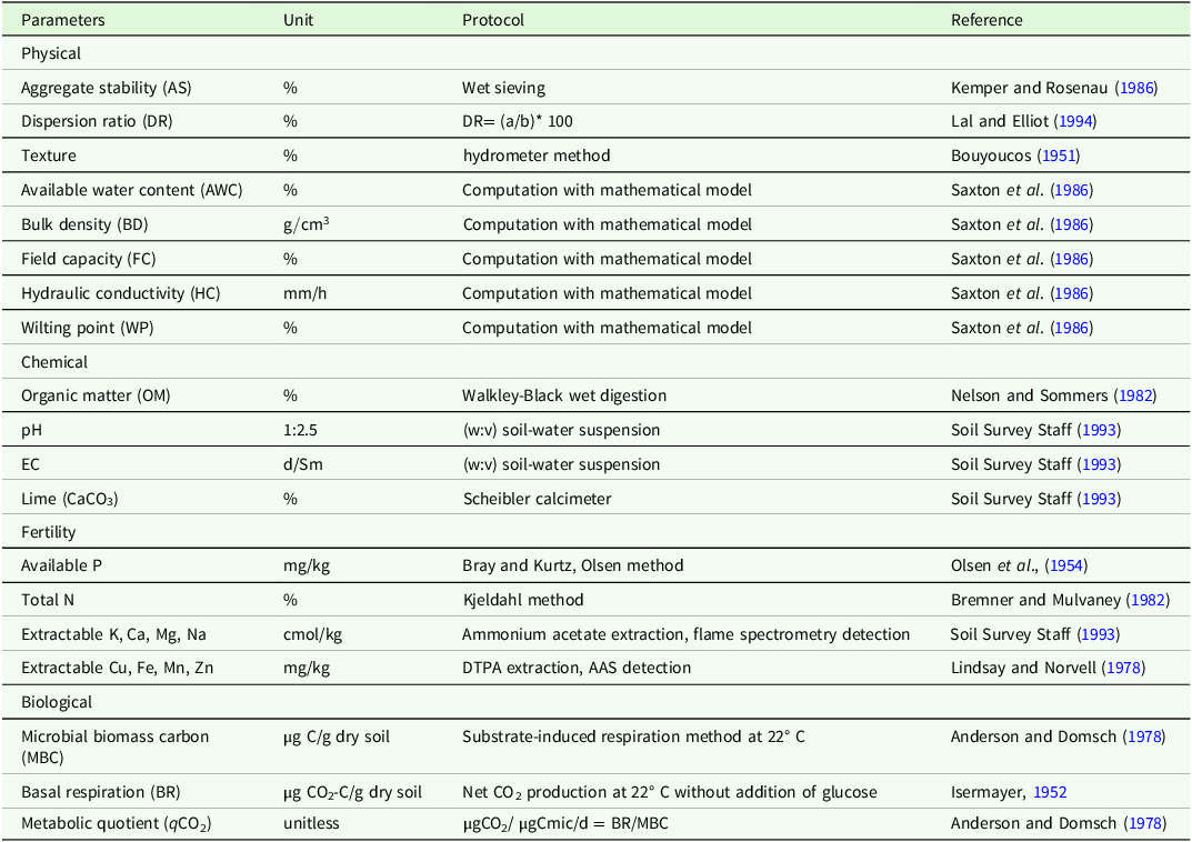
After cleaning, drying (air-dry), and grinding, the soil samples were passed through a 2 mm sieve. The soil’s physical, chemical, and biological properties were determined, and soil quality was calculated. A total of 27 soil properties were examined. In the SQI for hazelnut cultivation, the indicators are grouped under four categories and the physicochemical and biological analyses and methods of the soils used in the study are stated in Table 1.
Protocol measurements for indicators selected

EC, electrical conductivity; P, phosphorus; N, nitrogen; K, potassium; Ca, calcium; Mg, magnesium; Na, sodium; Cu, copper; Fe, iron; Mn, manganese; Zn, zinc; CO2, carbon dioxide a is the percentage of silt plus clay in suspension, b is the percentage of silt plus clay dispersed with chemical agent.
Determination of soil quality
The examined features were converted into unitless scores (xi) between 0 and 1, which can be compared with each other using linear and nonlinear scoring functions. The Analytic Hierarchy Process (AHP) was used to determine the weights (Wi) of the features. Soil quality was assessed using the linear combination method.
AHP is a multi-criteria decision-making method that enables numerical, hierarchical organization of parameters regarding their respective importance for solving the problem or achieving the objective of our interest. The pairs of individual indicators are compared to one another using arbitrarily assigned scales in a pairwise comparison matrix ranging from 1/9 to 9; where 9 represents the maximum importance of one indicator over another, 1 represents equal importance between indicators, and values less than 1 indicate a lesser importance of one indicator relative to another. The assigned values are based on experts’ experience. The upper triangular matrix is filled with assigned values from 1 to 9, whereas the lower triangular matrix is filled with the reciprocal values of the pairwise comparisons. The comparison scale thus includes the values: 9, 8, 7, …, 1/7, 1/8, and 1/9.
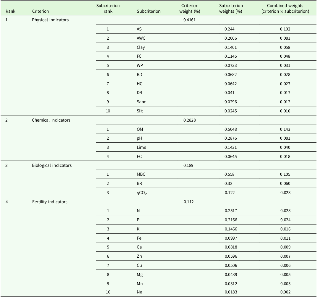
The matrix is then normalized by dividing each pairwise comparison value by the sum of the values in the corresponding column. The row averages of the normalized pairwise comparison matrix constitute the priority vector (weight scores) of the respective indicators. Lastly, the consistency of the obtained eigenvector should be checked by calculating the Consistency Ratio (CR). We multiply the pairwise comparison matrix by the eigenvector of the normalized matrix to yield a new vector. The second new vector is obtained by dividing each component of the second vector by its corresponding eigenvalue of the normalized matrix. The Random Index (RI) is also required to calculate the Consistency Ratio (CR). The RI values are generated by filling 100 matrices with dimensions corresponding to the total number of weighted indicators in our study and calculating the average of their coherence indicators (Saaty, Reference Saaty1980). A smaller CR indicates a more consistent comparison matrix. As a general rule, CR must be less than 0.1 for the indicator weightings to be considered consistent. The consistency is improved by better expert judgement when assigning importance scores, by fewer indicators, and by greater homogeneity of assigned scores (Saaty, Reference Saaty1993). Weights derived from soil quality indicators are shown in Table 2.
Weights of soil indicators with the Analytic Hierarchy Process (AHP) method

AS: Aggregate stability, AWC: Available water content, FC: Field capacity, WP: Wilting point, BD: Bulk density, HC: Hydraulic conductivity, DR: Dispersion ratio, OM: Organic matter, EC: electrical conductivity, MBC: Microbial biomass carbon, BR: Basal respiration, qCO2: Metabolic quotient, N: nitrogen, P: phosphorus, K: potassium, Fe: iron, Ca: calcium, Zn: zinc, Cu: copper, Mg: magnesium, Mn: manganese, Na: sodium.
Scoring of indicator values
Due to the different units of soil quality indicators, we normalized their values using standard scoring functions (SSF) before aggregating them into the SQI. The normalization assigns unitless scores ranging from 0 and 1 to the indicators using different scoring functions depending on each indicator’s functional effect on soil quality (Andrews et al., Reference Andrews, Karlen and Cambardella2004). A ‘more-is-better’ (MB) function is assigned to indicators for which higher values indicate better soil quality. A ‘less is better’ (LB) function describes the opposite relationship where low indicator values contribute to better soil quality. For some of the indicators, an optimal range was delimited by assigning them MB and LB functions depending on whether the indicator value was above or below the optimal range (Andrews et al., Reference Andrews, Karlen and Cambardella2004).
We used linear and nonlinear approaches for standard scoring. For linear SSF, we followed the equations used in Fernández et al. (Reference Fernández, Keshavarzi, Rodrigo-Comino, Schnabel, Contador, Gutiérrez and Cerdà2020) (Equations 1 and 2). The non-linear approach using a sigmoid function, with a curve slope of −2.5, was adapted from the paper by Bastida et al. Reference Bastida, Moreno, Hernández and García2006 (Equations 3 and 4). The SSF equations are presented below:
 $$MB\; = \;{{{0,9\; \times \;\left( {x - L} \right)}}\over{{\left( {U - L} \right)}}} + 0,1$$
 $$LB\; = \;{{{1 - 0,9\; \times \;\left( {x - L} \right)}}\over{{\left( {U - L} \right)}}}$$
 $$MB_{NL}={{1}\over{1+{(x/\overline{x})}^{-2,5}}}$$
 $$LB_{NL}={{1}\over{1+{(x/\overline{x})}^{2,5}}}$$
where MB represents linear ‘more is better’ function,
 $M{B_{NL}}$
represents non-linear ‘less is better’ function, LB represents linear ‘less is better’ function,
 $L{B_{{\rm{NL}}}}{\rm{\;re}}$
presents non-linear ‘less is better’ function, x is indicator value, is mean indicator value, U is upper limit of indicator values and L lowest indicator values.
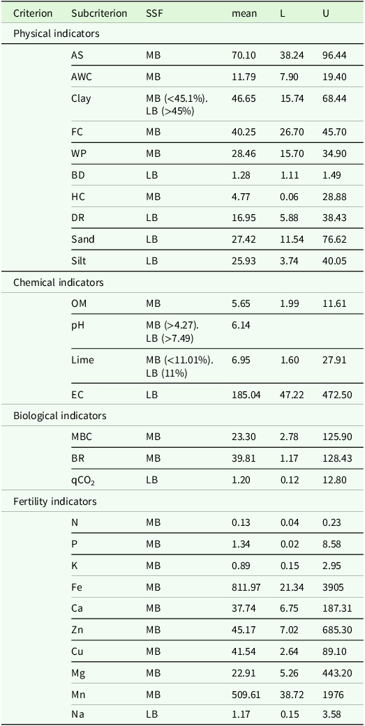
The assignment of the types of SSF to the respective soil indicators, as well as their mean, upper, and lower values, is presented in Table 3. All the indicators were calculated using both linear and non-linear approaches.
The types of standard scoring functions (SSF) assigned to each of the soil quality indicator

MB refers to ‘more is better’ SSF, LB refers to ‘less is better’ SSF, mean represents mean indicator values, L is minimum and U the maximum indicator value. AS: Aggregate stability, AWC: Available water content, FC: Field capacity, WP: Wilting point, BD: Bulk density, HC: Hydraulic conductivity, DR: Dispersion ratio, OM: Organic matter, EC: electrical conductivity, MBC: Microbial biomass carbon, BR: Basal respiration, qCO2: Metabolic quotient, N: nitrogen, P: phosphorus, K: potassium, Fe: iron, Ca: calcium, Zn: zinc, Cu: copper, Mg: magnesium, Mn: manganese, Na: sodium.
Integration of indicators with soil quality index
The indicator values were combined into a single index ranging from 0 to 1, with higher values indicating greater soil quality. The SQI was calculated using the weighted additive method, as presented in the formula below (Equation 5):
 $$SQI = \;\mathop \sum \limits_{i = 1}^n ({S_L} \times {W_i})$$
where SQI represent Soil Quality Index with weights assigned by AHP and scores calculated with linear and nonlinear SSF,
 ${S_L}$
represents sub-criteria’s normalization score calculated with linear and non-linear SSF respectively,
 ${W_i}$
is a weight value of the parameter previously determined by AHP method and n is a total number of parameters.
Geostatistical interpolation and statistical approaches
Spatial distribution maps of indicator-value data and of the values for four SQI were generated using ArcGIS v10.7. The spatial prediction from the sampling points’ data was interpolated across the delimited study area using inverse distance weighting (IDW) geostatistical model (power = 2) and a radial basis function (thin-plate spline). To separate spatially predicted values into several classes of maximal dissimilarity, the Jenks natural breaks classification method (Jenks, Reference Jenks1967) was applied.
The PCA was applied to the data to create a MDS of soil properties. When determining parameters for inclusion in the MDS, component loadings from PCA, correlation-load totals, and inter-data correlation analyses will be considered. Descriptive statistics for soils and PCA will be performed using IBM SPSS 23 software package. In the PCA, soil properties will be standardized, and the Kaiser-Meyer-Olkin (KMO) measure and Bartlett’s test of sphericity will be examined to assess the suitability of the data for factor analysis. Principal components (PC) with eigenvalues greater than 1 will be selected and the MDS will be created by examining the correlation matrices. Tukey’s multiple-comparison test was used to compare the soil quality approaches. The boxplot and clustering dendrogram were obtained using the IBM SPSS 23 software package. The correlation matrices among the studied soil-quality models were calculated using the METHANE package in R.
The XGBoost package in R was used to implement the XGBoost algorithm to estimate soil quality. The model can be expressed mathematically (Equation 6):
 $$\widehat {y\;}i = \;\mathop \sum \limits_{k = 1}^k {f_k}\left( {{x_i}} \right),\;{f_k} \in F\;$$
where F is the set of all potential regression trees, K is the number of trees, and f is a function in the functional space F. Consequently, the optimization’s goal can be expressed as follows (Equation 7):
 $$obj\left( \theta \right) = {\rm{\;}}\mathop \sum \limits_i^n {\rm{l}}\left( {{y_i},{\rm{\;}}\widehat {{y_i}}} \right){\rm{\;}}\mathop \sum \limits_{k = 1}^k {f_k}\left( {{f_k}} \right)$$
where the regularization term is Ω(fk) and the training loss function is I(yi, yi). The XGBoost model’s objective is to minimize obj(Ø). Several tests revealed that shrinkage (eta), maximum depth (max_depth), number of iterations (nround), and alpha, set to 0.8, 10, 200, and 0.2 respectively, stabilized prediction error in the XGBoost algorithm. To improve learning, the k-fold cross-validation method was also used, with validation performed on 70% of the training data. This validation method prevented overfitting of the model to the training data set. Following multiple randomized tests, 10-fold cross-validation was found to be the most successful method. Basic soil properties (sand, silt, clay, pH, EC, organic matter (OM), lime content, N, P, and K) were used as input to the models.
Root mean square error (RMSE), mean absolute error (MAE), mean absolute percentage error (MAPE), coefficient of determination (R2), and Lin’s concordance correlation coefficient (LCC) were used to evaluate the models.
Results
Physico-chemical, productivity and biological properties of soils
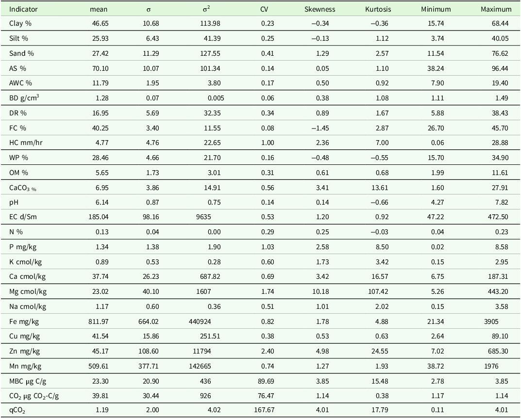
The soil characteristics of 116 hazelnut plantations sampled in our study area vary due to the diverse parent material, environmental factors, different degrees of soil formation and leaching processes, and plantation management activities (e.g. fertilization, liming, soil cultivation, etc.). Descriptive statistics for soil properties are presented in Table 4. Values of most physical indicators were normally distributed except for hydraulic conductivity (HC), whose high kurtosis indicates a heavy-tailed distribution caused by outliers. Soil particle-size distribution classes in the samples range from heavy to moderate clay, coarse to fine silt, and very coarse to fine sand texture classes. The mean soil texture-class values indicate a heavy texture for clay and a moderate texture for silt and sand. The maximum relative contents of clay and sand in the soil samples were 68.44% and 76.62%, respectively. The mean values for AS, BD and DR are 70.1%, 1.28
 ${\rm{g}}/{\rm{c}}{{\rm{m}}^3}$
and 16,95% which correspond to high AS, low BD and slight dispersion percentage rate as suggested by Hazelton and Murphy (Reference Hazelton and Murphy2016). All analysed samples exhibit AS values rated as highly stable. Water retention properties vary with sample texture. The ranges were 7.90–19.4% for available water content (AWC), 26.7–45.7% for field capacity (FC), 15.7–34.9% for wilting point (WP), and 0.06–28.88 mm/h for HC; their mean values were 11.79% for AWC, 40.25% for FC, 28.46% for WP, and 4.77 mm/h for HC. The mean HC value is rated very low according to Hazelton and Murphy (Reference Hazelton and Murphy2016). Chemical indicator values range from 1.99–11.61% for OM, 1.99–27.91% for lime content, pH 4.27–7.82, and EC 47.22–472.5 µS/cm. Their values, with the exception of lime content, are normally distributed. The mean OM content is 5.65%, which, according to the rating proposed by Hazelton and Murphy (Reference Hazelton and Murphy2016), is considered extremely high. The OM content in all samples ranged from moderate to extremely high levels. pH values range from mildly alkaline to very strongly acidic, with a mean pH of 6.14 (slightly acidic). The lime content, however, was found to be between 1.6% and 27.91%, with a mean of 6.75%, which is considered moderate. The EC values are rated non-saline to slightly saline (Hazelton and Murphy Reference Hazelton and Murphy2016); the mean value is 185.04 µS/cm.
Statistical description of soil indicators

Indicators’ values including mean value (mean), standard deviation (σ), variance (σ2), coefficient of variation (CV), skewness, kurtosis, range, minimum and maximum values. AS: Aggregate stability, AWC: Available water content, BD: Bulk density, DR: Dispersion ratio, FC: Field capacity, HC: Hydraulic conductivity, WP: Wilting point, OM: Organic matter, CaCO3: lime, EC: electrical conductivity, N: nitrogen, P: phosphorus, K: potassium, Ca: calcium, Mg: magnesium, Na: sodium, Fe: iron, Cu: copper, Zn: zinc, Mn: manganese, MBC: Microbial biomass carbon, CO2-BR: Basal respiration, qCO2: Metabolic quotient.
Indicator values of nutrients in the soil were generally normally distributed, except for Ca, Mg, and Zn, which exhibited heavy-tailed, skewed distributions. Total nitrogen in the soil ranged from very low (0.04%) to medium (0.23%), with the mean value being low (0.13 mg/kg) (Hazelton and Murphy, Reference Hazelton and Murphy2016). Available phosphorus levels were very low (0.02 mg/kg) and low (8.58 mg/kg), and its mean value of 1.34 mg/kg was considered very low (Hazelton and Murphy, Reference Hazelton and Murphy2016). Potassium values between 0.15 and 2.95 cmol/kg correspond to content levels ranging from low to very high. A mean potassium concentration of 0.89 cmol/kg is considered high. The values of the remaining macronutrients (Ca, Mg, and Na) range from 6.75 to 187.31 cmol/kg, 5.26 to 443.2 cmol/kg, and 0.15 to 3.58 cmol/kg, respectively. The levels of Ca range from moderate and very high, with its mean value (37.74 cmol/kg) at the very high level. The Mg content is between high and very high, while the Na content is between low and very high, with its mean value being at a high level (Hazelton and Murphy, Reference Hazelton and Murphy2016). The values of micronutrients are unusually high and reach levels that can be harmful to the plants, as the case of the maximum Zn value of 685.3. The values of biological factors range from 2.78 to 125.9 μg C/g soil for MBC and from 1.17 to 128.43 μg C/g soil for BR. Adapting the rating proposed by Andrews et al. (Reference Andrews, Karlen and Cambardella2004) and Vasconcellos et al. (Reference Vasconcellos, Bonfim, Andreote, Mendes, Baretta and Cardoso2013), all the MBC values are rated as low; basal respiration values range from low to high, whereas the mean BR value is considered low.
Generating a minimum data set
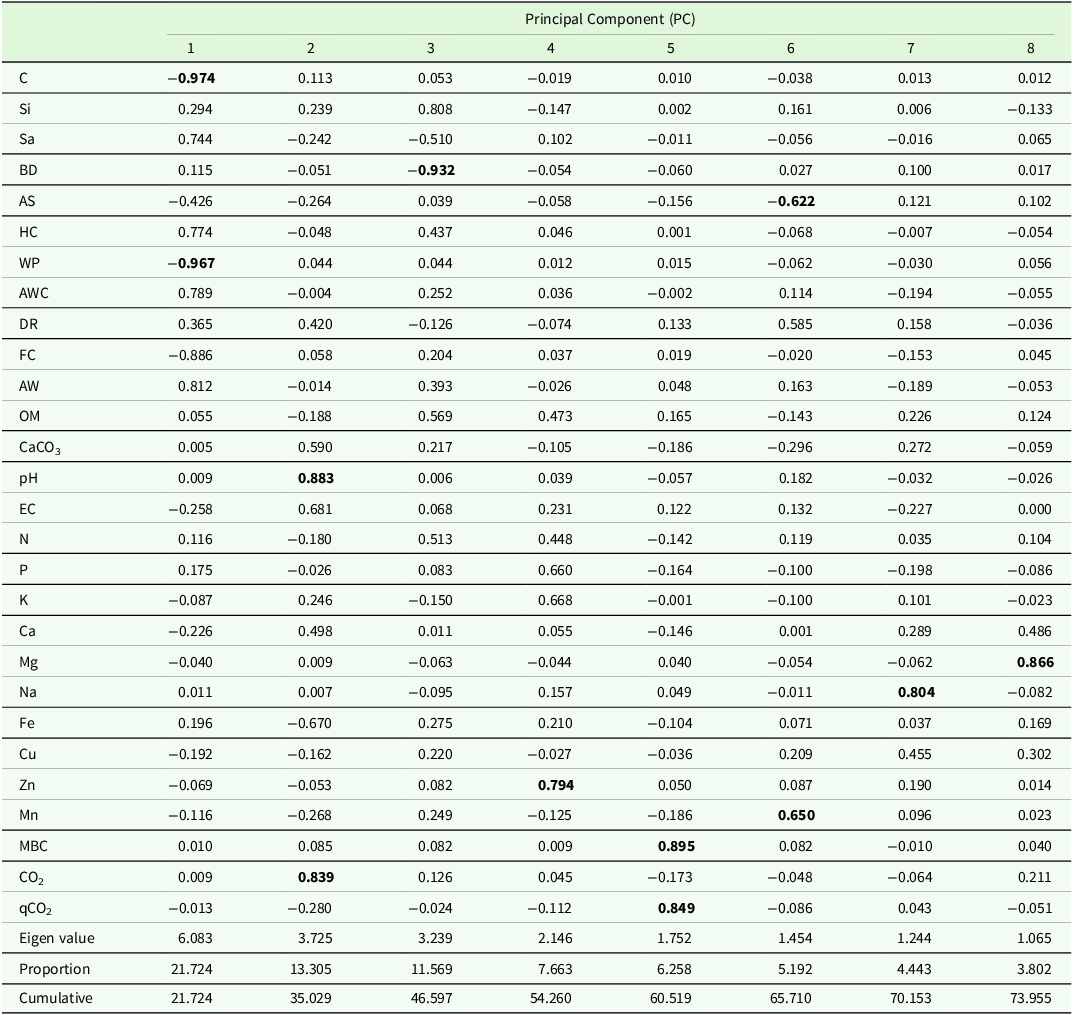
To ensure the sustainability of hazelnut cultivation and to determine the SQI, selecting the most appropriate soil indicators is essential. In this study, we evaluated 27 factors in the total data set (TDS) to best represent soil physical, chemical, biological, and fertility properties. We used PCA to generate this MDS (Nabiollahi et al., Reference Nabiollahi, Taghizadeh-Mehrjardi, Kerry and Moradian2017; Qi et al., Reference Qi, Darilek, Huang, Zhao, Sun and Gu2009; Saygın et al., Reference Saygın, Şavşatlı, Dengiz, Yazıcı, Namlı, Karataş, Şenol, Akça, Pacci, Karapıçak, Ay and Demirkaya2023). The PCA performed to derive a MDS of soil properties is presented in Table 5. During the creation of the MDS using the PC method, the KMO sphericity test was applied. The results were determined to be statistically significant (KMO > 0.5). In the evaluation using PCA, PCs with an eigenvalue ≥1.0 were retained to include the indicators in the MDS. With an eigenvalue ≥1.0, eight PC were considered. A total of 73.95% of the variance was explained by 8 PC. In each PCA with an eigenvalue ≥1.0, indicators falling within 10% of the highest weight were evaluated for the MDS. When more than one variable from the same PC that met the indicator selection criteria were entered into the data set and the correlation between those variables was ≥0.60, the variable with the highest weight was selected for the MDS. The features with the highest weights in PCA1 were identified as clay and WP. The selected features showed high correlation (≥0.60) with each other. Clay was determined as the feature with the highest weight and was considered as the indicator included in the MDS. In PCA2, pH and CO2 have high weights. It exhibited a high correlation (r = 0.68) with pH-CO2. The feature with the highest weight is pH, and pH-related features are included in the MDS. The features with the highest weights in PCA3 and PCA4 were identified as BD and Zn and were included in the MDS. In PCA5, MBC and qCO2 were selected as features with high weights; because they were highly correlated, qCO2 was eliminated and MBC was added to MDS. Features with high loadings on other PC were not identified. 27 indicators were subjected to PCA, resulting in a MDS comprising nine indicators.
Principal component analysis matrix of soil properties

C: clay, Si: Silt, Sa: sand, BD: Bulk density, AS: Aggregate stability, HC: Hydraulic conductivity, WP: Wilting point, AWC: Available water content, DR: Dispersion ratio, FC: Field capacity, OM: Organic matter, CaCO3: lime, EC: electrical conductivity, N: nitrogen, P: phosphorus, K: potassium, Ca: calcium, Mg: magnesium, Na: sodium, Fe: iron, Cu: copper, Zn: zinc, Mn: manganese, MBC: Microbial biomass carbon, CO2-BR: Basal respiration, qCO2: Metabolic quotient.
Soil quality and statistical comparisons
The boxplots showing the minimum and maximum values of the soil-quality approaches are shown in Figure 4. In addition, the results of cluster analysis of SQIs obtained using different approaches are presented in Figure 5.
Box-Plot graphics. TDS: total data set, MDS: minimum data set, L: Linear, NL: Non-Linear, CON: Conventional hazelnut farming, ORG: Organic hazelnut farming.

Clustering analysis. SQI: soil quality index, TDS: total data set, MDS: minimum data set, L: Linear, NL: Non-Linear, CON: Conventional hazelnut farming, ORG: Organic hazelnut farming.

SQI values ranged from 0.331 to 0.577 for TDS-ORG-L and from 0.334 to 0.587 for the nonlinear method. Using the MDS, MDS-ORG-L ranged from 0.211 to 0.591, and the non-linear method ranged from 0.290 to 0.580. In conventional agricultural areas, SQI values obtained using the TDS with linear and non-linear methods were 0.314-0.622 and 0.304–0.587, respectively; using the MDS they were 0.211–0.606 and 0.290–0.589, respectively. The lower and upper outliers with the greatest deviation from the normal distribution were detected by the MDS-ORG-NL method. A 96.38% statistical similarity was detected between the total data set linear SQI for conventional hazelnut cultivation (TDS-CON-L) and the total data set non-linear SQI (TDS-CON-NL), while a 91.60% statistical similarity was detected between the total data set linear SQI for organic hazelnut cultivation (TDS-ORG-L) and the total data set non-linear SQI (TDS-ORG-NL) (Figure 5). In addition, a 65.55% statistical similarity was observed between conventional and organic hazelnut cultivation.
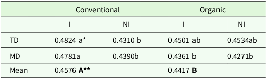
The changes in SQIs obtained by TDS and MDS, using linear and nonlinear methods for conventional and organic cultivation are presented in Table 6. The average soil quality in conventional hazelnut cultivation was 0.4576, compared with 0.4417 in organic hazelnut cultivation; this difference was statistically significant. In addition, SQI values determined by linear and nonlinear methods for conventional hazelnut cultivation and for the TDS were statistically different (0.4824–0.4310), whereas SQI values for organic hazelnut farming determined by linear and nonlinear methods were statistically similar (0.4501–0.4534). When SQI values obtained from MDSs were examined using linear and nonlinear methods, they yielded similar results.
Soil quality index (SQI) variation due to the difference in cultivation and approaches (Linear and Non-linear)

* The change due to the difference in the method and data set is statistically significant (P < 0.01), ** The change in SQI due to the difference in cultivation is statistically significant (P < 0.05), L: Linear, NL: non-linear, TD: total data set, MD: minimum data set.
Correlation matrices showing the relationships between SQI values obtained by different methods and yield values are shown in Figures 6 and 7. Correlation matrices indicated a positive relationship between SQI values obtained by different methods (linear and non-linear) and yield. A statistically significant positive correlation was observed between the SQI values from the TDS of conventional hazelnut cultivation soils and yield (r = 0.51, p < 0.05). In addition, the same results were obtained for soils used for organic hazelnut cultivation. Moreover, the highest positively correlation was found between TDS-SQI-ORG-L and yield values (r = 0.56, p < 0.001)
Relationship between SQI values of conventional hazelnut cultivation and yield Values. SQI: soil quality index, TDS: total data set, MDS: minimum data set, L: Linear, NL: Non-Linear, CON: Conventional hazelnut farming.

Relationship between SQI values of organic hazelnut cultivation and yield values. SQI: soil quality index, TDS: total data set, MDS: minimum data set, L: Linear, NL: Non-Linear ORG: Organic hazelnut farming.

Prediction and spatial distribution of SQI
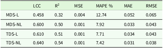
Model evaluation parameters are stated in Table 7. The lowest LCC and R2 values when estimating soil quality using basic soil properties (sand, silt, clay, lime, OM, pH, EC, N, P, K) with the XGBoost algorithm were observed in the MDS-L data set: 0.458 and 0.32, respectively. Although MAPE differed by approximately 5% when soil quality was estimated using linear versus nonlinear methods with the MDS data set, error levels in the TDS data set were very similar. RMSE values for the predictions obtained with the MDS-NL and TDS-L data sets were 0.043. The most influential features for model prediction were identified as N (0.189), K (0.020), OM (0.010), P (0.008), and pH (0.004) (Figure 8).
Model evaluation parameters

LCC: Lin’s concordance correlation coefficient, MSE: mean square error, MAPE: mean absolute percentage error, MAE: Mean absolute error, RMSE: Root mean square error, MDS-L: the minimum data set linear SQI, MDS-NL: the minimum data set non-linear SQI, TDS-L: the total data set linear SQI, TDS-NL: the total data set non-linear SQI.
Importance of soil properties OM: organic matter, LC: Lime content, Si: Silt, C: Clay, Sa: Sand, EC: electrical conductivity.

Spatial distribution maps of the SQI values for TDS and MDS, generated using linear and non-linear approaches for both conventional and organic hazelnut farming, are presented in Figure 9. In the study, the obtained results indicated that TDS-CON-L, MDS-CON-NL, and MDS-CON-L approaches showed a similar pattern to each other (except for the map of TDS-CON-NL). This is also apparent from the clustering dendrogram in Figure 5. In addition, the distribution maps of SQI values (TDS-ORG-L and TDS-ORG-NL) exhibited a similar pattern, whereas those of MDS-ORG-L and MDS-ORG-NL exhibited a different pattern. High-quality soils in hazelnut cultivation are located in the northern and northwestern parts of the study area (Şengüven, Esentepe, and Aşağıgüney villages), whereas low-quality soils in hazelnut-growing areas are found in the mountainous southern part of the study area.
Spatial distribution maps of the Observed (OBS) and Predicted (PRE) values of SQI for total data set (TDS) and minimum data set (MDS) with Linear (L) and Non-Linear (NL) approaches.

Spatial distribution maps of observed and predicted SQI values for TDS and MDS, obtained using linear and nonlinear approaches, are shown in Figure 9. The distribution maps for TDS-OBS-L, TDS-PRE-L, and TDS-PRE-NL exhibit similar spatial patterns across the study area, except for the TDS-OBS-NL map. The MDS-PER-L, MDS-PER-NL and MDS-OBS-NL maps have almost identical distributions, except for the MDS-OBS-L map.
Discussion
The foundation of all agricultural productivity is soil. Therefore, improving soil fertility and quality is the first step towards achieving the required quantity and quality of a product. Plant nutrients are among the most crucial elements for boosting soil fertility, but it is critical to preserve the soil’s chemical, physical, and biological properties (Alaboz et al., Reference Alaboz, Odabas and Dengiz2023; Şenol et al., Reference Şenol, Alaboz, Demir and Dengiz2020). The results indicate that OM content and topsoil OM stocks are, on average higher under organic management (Gattinger et al., Reference Gattinger, Muller, Haeni, Skinner, Fliessbach, Buchmann and Niggli2012; Lorenz and Lal, Reference Lorenz and Lal2016). OM is particularly important for soil quality, as it reduces nutrient leaching and promotes soil aggregation, which improves soil structure, thereby reducing soil erodibility (Lynch, Reference Lynch, Martin and MacRae2014) and increasing water-holding capacity (Gomiero et al, Reference Gomiero, Pimentel and Paoletti2011). Although evidence supports the claim that organic agriculture leads to improvements in some soil properties lowers greenhouse gas emissions, enhances air and water quality, and consumes less energy, organic farming areas cover only a small fraction of cultivated land (9.4% in the EU and 1.5% globally in 2020) (Lorenz and Lal, Reference Lorenz and Lal2016). The major drawback of organic farming is its yields, which are on average 19% lower compared with more intensive agricultural practices. Nonetheless, organic farming holds significant potential to reduce the environmental impact of food production, and its methods could contribute to a sustainable intensification of agricultural systems in the future (Lorenz and Lal, Reference Lorenz and Lal2016).
The soil is a complex, heterogeneous system characterized by closely interrelated physical, chemical, mineralogical, and pedological properties, as well as individual characteristics. Consequently, its management should encompass all of these aspects. Conversely, the absence of such a mechanism can result in irreversible errors, as previously highlighted by Delgado and Gómez (Reference Delgado and Gómez2024). The efficient and sustainable use of soils is possible only by determining, using appropriate methods, the limiting factors that affect productivity and the properties affecting sustainability. The conventional approach has been predicated on analysis of specific properties and their compatibility with various criteria, employing designated tools for each property and measuring positive or negative correlations among these properties. Despite the development of fertilization programs based on analysis, this practice, in its current form, is inadequate to maintain or improve plant productivity and production. Soil is an intricate system characterized by numerous sources of variability. It is imperative to recognize that evaluating soil solely in terms of nutrient content, while beneficial, is an incomplete assessment that fails to guarantee productivity or sustainability.
The study’s assessment of physical and chemical properties revealed variability resulting from dynamic interactions between human activities, such as fertilizer management, and environmental factors, such as the degree of soil development and leaching processes. Sandy clay loam, loam, sandy loam, and clay loam were the texture classes identified in the medium-fine and coarse texture groups of soils used in this study. The FC and AWC values of catchment soils are generally low due to their coarse texture. These results are also consistent with those reported by Mihalikova et al. (Reference Miháliková, Özyazıcı and Dengiz2016). Furthermore, a range of microbial-response parameters, including microbial biomass carbon, basal respiration, and metabolic quotient, are frequently used to assess the stabilization of soil OM, soil aggregation, and soil quality, and to monitor soil formation (Ashraf et al., Reference Ashraf, Waqas and Rahman2022). One of the most significant factors in this regard is microbial activity involved in acquiring energy and nutrients, including OM (organic carbon) and elements such as N, P, K, Ca, and Mg. In the present study, MBC demonstrated the greatest variability among the selected biological indicators. Electrical conductivity values were low, indicating ‘non-saline’ soils, whereas pH values in soil samples ranged from strongly acidic to mildly acidic. Furthermore, the average CaCO3 content in each soil sample is less than 2%. As a result, the CaCO3 level of the soils in the research area was categorized as ‘low’, while their OM content ranged from ‘low’ to ‘high’. Additionally, several soil samples had adequate micronutrient concentrations, as indicated by their mean concentrations. Elevated mobility of micronutrients was observed in the soil solution at acidic pH. Additionally, it might be related to the very low concentrations of leachable calcium carbonate. Similar results were found in several studies conducted in the Black Sea region, including Sayğın et al. (Reference Saygın, Gürsoy, Demirağ Turan and Dengiz2017).
The XGBoost model demonstrated higher simulation accuracy and greater generalization capability (Liu et al., Reference Liu, Li, Wu, Shi, Zhao, Wu and Wang2023). Various nonlinear models have been widely used for estimation, including extreme gradient boosting machine (XGBoost), backpropagation neural network (BPNN), and random forest (RF) (Huang et al., Reference Huang, Wang, Baishan and An2023, Yang et al., Reference Yang, Feng, Son, Wang, Yang, Xie, Ji, Xiao, Zhang, Song and Saleem2021). In terms of their estimation ability, the three estimation models could be ranked as follows: XGBoost > BPNN > RF. In particular, CWT–XGBoost, combined with the six feature-variable algorithms, provided excellent results, with its RPD ranging from 2.14 to 2.78 (Yang et al., Reference Yang, Li and Ma2023). In terms of model selection, Yu et al. (Reference Yu, Zhou, Wang, Xiao, Peng, Li and Li2024) provided support for the advantage of XGBoost in capturing complex relationships and working with heterogeneous data. Zhao et al. (Reference Zhao, Li, Li, Li and Yang2024) reported that XGBoost provided high accuracy and stability in soil salinity estimation, demonstrating particularly strong performance when combining spectral and texture data. However, they noted that overfitting, interpretability, and regional generalizability should be considered cautiously, and that testing in different geographies would be a key area for future research.
In this study, nitrogen (N), potassium (K), OM, phosphorus (P), and pH were identified as the most influential variables in model predictions (Figure 10). These variables are known to be key determinants of soil fertility and ecosystem functioning. Nitrogen and phosphorus are essential macronutrients vital for plant growth and microbial activity, while potassium plays a critical role in osmotic balance and enzymatic processes. OM improves soil physical structure, water holding capacity, and nutrient cycling, while pH directly affects plant uptake of nutrients and microbial activity. These findings are consistent with previous studies that conducted similar machine-learning-based soil-quality assessments (Lee and Lee, Reference Lee and Lee2024; Trontelj ml and Chanbersi, Reference Trontelj Ml and Chambers2021), demonstrating that these variables are reliable indicators of the chemical and biological dimensions of soil quality. All nutrients, except nitrogen, largely originate from the lithosphere and enter soil nutrient cycles via various soil-forming processes, while nitrogen enters the soil through precipitation, OM mineralization, biological fixation, and addition as fertilizers. The latter is required, above all, in agricultural systems where the intensive plant production far exceeds the amount of vital nutrients stored in the soil. Generally, the limiting factor for plant production is nitrogen, followed by phosphorus and potassium. These vital elements are normally added to the soil in synthetic form. Since their concentrations and availability can change over small-time scales, they are considered dynamic indicators of soil quality.
Importance of soil properties. OM: organic matter, LC: Lime content, Si: Silt, C: Clay, Sa: Sand, EC: electrical conductivity.

The gain metric, which quantifies the relative contribution of each feature to the model, was used to assess the importance of XGBoost features (Liang et al., Reference Liang, Jiang, Yan and Chen2021). It appears that the XGBoost algorithm can forecast local soil variability and account for the impact of aggregation. Like other models, XGBoost is heavily reliant on the resolution and quality of the input data, yet it was only partially successful in modelling variability (Zeitfogel et al., Reference Zeitfogel, Feigl and Schulz2023). The high significance of these variables in the XGBoost model may be due to the nonlinear and interactive relationships between these parameters and soil fertility indicators. However, as the relative importance of features may vary depending on soil type, local weather conditions, and land use history, it will be important for future studies to validate these findings across different regions and with larger data sets. In this study, various approaches were tested to improve the model’s accuracy. The aim of this study was to determine the feasibility of prediction using basic soil properties readily measured in the laboratory. However, the predictive accuracy is expected to increase by evaluating different parameters, especially those from remote sensing. The outcome shows that XGBoost successfully predicted soil attributes using remote sensing indices, indicating that machine learning techniques can be improved by using remote sensing data to enable field-to-regional-scale spatial prediction of soil attributes (Sahabiev et al., Reference Sahabiev, Smirnova and Giniyatullin2021). Furthermore, Song et al. (Reference Song, Zhao, Su, Li, Hu and Cui2018) noted that regional-scale forecasts of soil property variability are significantly enhanced when multispectral and hyperspectral remote sensing data are combined with machine-learning models.
Conclusions
In this study, soil quality in areas where hazelnuts are produced under conventional and organic agriculture was evaluated. Additionally, the predictability of soil quality was assessed using the XGBoost algorithm. Soil quality in conventional agriculture was found to be higher than in organic farming areas. With the XGBoost algorithm, soil quality can be estimated with approximately 60% accuracy. Additionally, macro elements and OM were considered important features in estimating soil quality. Although soil quality was determined to be higher under conventional agricultural practices in this study, the effects of organic fertilizer applications will persist for many years, allowing the study to continue. In this study, basic soil properties were evaluated to facilitate application in model evaluation. In the study, it can be considered a parameter that limits the accuracy of the model. In a subsequent study, the model’s predictive performance will be evaluated across different soil properties. Additionally, the use of only soil analyses in the study can be considered a limiting factor for the model. It is planned to carry out more comprehensive studies using reflectance’s using remote sensing technologies.
Data availability statement
Data available on request.
Acknowledgements
An AI tool was used to improve the language.
Funding statement
This research has not found any sources.
Author contributions
O. DENGİZ: Conceptualization, Methodology, Sample collection, Data processing, Writing, Supervision, S. PACCi: Sample collection and analysis, Data processing, Writing P. ALABOZ: Conceptualization, Methodology, Data processing, Writing, N. SUBAN: Sample collection and analysis, Data processing, Writing. All authors read and approved the final manuscript.
Competing interests
The authors declare no competing interests.