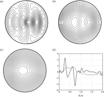
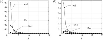
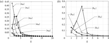
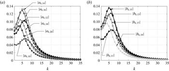
1 Introduction
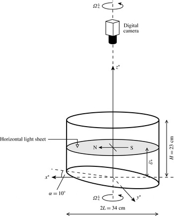
In a pioneering paper, Pedlosky & Greenspan (Reference Pedlosky and Greenspan1967) examined how a rotating, homogeneous fluid is spun-up inside a sliced cylinder – a closed, vertical cylinder with its base plane inclined at an angle
 $\unicode[STIX]{x1D6FC}$
to the horizontal (see figure 1). The relevance of this problem, of course, is as a model to the dynamics in a mid-latitude ocean basin large enough to require the inclusion of the
 $\unicode[STIX]{x1D6FD}$
effect. Rossby waves are much in evidence in the results, as two-dimensional vorticity waves that propagate across the slope and eventually fill the fluid’s interior, resulting in spin-up. Pedlosky & Greenspan (Reference Pedlosky and Greenspan1967, pp. 303 and 304) make the comment that ‘…many similar problems can be formulated in this (sliced cylinder) configuration which are of geophysical relevance’ and that ‘…the introduction of density stratification …would undoubtedly produce many significant new effects’. In this paper we will consider how the spin-up mechanism and formation of Rossby waves in a sliced cylinder are affected by the introduction of a linear density stratification, a problem that has remained unresolved since publication of Pedlosky and Greenspan’s classical paper.
A sketch of the experiment set-up.

The mechanism described by Pedlosky & Greenspan (Reference Pedlosky and Greenspan1967) is in stark contrast to how spin-up is achieved in a regular cylinder (
 $\unicode[STIX]{x1D6FC}=0$
). In that case, the spin-up is accomplished by inward convection of angular momentum that has been transported into thin, viscous layers on the vertical sidewalls of the container (Stewartson Reference Stewartson1957; Greenspan & Howard Reference Greenspan and Howard1963; Greenspan Reference Greenspan1968). That angular momentum has its origin in the top and bottom Ekman layers, wherein spun-up fluid is transported radially outwards and erupts from the upper and lower corners of the container into the sidewall shear layers. This description does not, of course, apply to a fluid that is density stratified. Walin (Reference Walin1969) showed that in the presence of a stable linear stratification, the fluid’s density field inhibits vertical motions and vortex stretching, and so the secondary circulations just described are not present. Instead the Ekman-layer fluid erupts directly into the inviscid core, penetrating to a height above the base (or depth below the lid) that scales with
 $S^{-1/2}$
, where
 $S=(N/\unicode[STIX]{x1D6FA})^{2}$
is the Burger number,
 $N$
the fluid’s buoyancy frequency and
 $\unicode[STIX]{x1D6FA}$
the container’s angular frequency. For general overviews of spin-up, see Benton & Clark (Reference Benton and Clark1974) and Duck & Foster (Reference Duck and Foster2001).
More recently, spin-up problems have been studied in a range of non-axisymmetric (constant depth) containers. What results are quite different spin-up morphologies, depending on the container’s geometry. The first such investigation seems to be that of van Heijst (Reference van Heijst1989), who examined homogeneous spin-up in a semi-circular cylinder, and a circular cylinder with a radial barrier. Subsequent to this, van Heijst and colleagues found much more complicated spin-up mechanisms in cuboid containers, using both homogeneous and linearly stratified fluids (van Heijst, Davies & Davis Reference van Heijst, Davies and Davis1990; van Heijst, Maas & Williams Reference van Heijst, Maas and Williams1994). In the latter reference the bottom boundary was also sloped, as in Pedlosky & Greenspan (Reference Pedlosky and Greenspan1967). In all of these studies, intense vortices with axes parallel to the rotation axis are seen to form in the fluid’s interior, which are as a result of unsteady separation of the sidewall boundary layers, a mechanism that was studied in detail for the case of a square cylinder by Munro, Hewitt & Foster (Reference Munro, Hewitt and Foster2015). Of course, these vortices are in stark contrast to the long-slope propagating vorticity waves that form in the sliced cylinder, which are a result of vortex stretching.
In Munro & Foster (Reference Munro and Foster2014), the authors examined the spin-up of a linearly stratified fluid in a sliced cylinder with a square cross-section, using both asymptotic and experimental approaches to ascertain the different mechanisms that result in spin-up compared to the case of a square cylinder with a flat bottom (
 $\unicode[STIX]{x1D6FC}=0$
), which was studied earlier by Foster & Munro (Reference Foster and Munro2012). The results are that the Rossby waves decay very rapidly in the entire water column, and much more rapidly when the Burger number,
 $S=(N/\unicode[STIX]{x1D6FA})^{2}$
, is greater than one. If
 $H$
is the container depth and
 $\unicode[STIX]{x1D708}$
the kinematic viscosity, then we determined that, after a few ‘spin-up times’, multiples of
 $H/(\unicode[STIX]{x1D708}\unicode[STIX]{x1D6FA})^{1/2}$
, the Rossby waves have decayed, and the interior is partially spun-up, with precisely the same azimuthal velocity variation with radius and height as in the flat-bottom case (Foster & Munro Reference Foster and Munro2012). In both cases, the eruption of the Ekman layers, at the vertical sidewalls, play a crucial role in the process. We found that the Rossby-wave frequencies are bounded above by
 $S^{1/2}$
, and determined numerical values for frequencies for representative Rossby waves. What was surprising is that the actual spin-up time is shorter in the presence of the sloping bottom boundary: if we take the bottom slope,
 $\unicode[STIX]{x1D6FC}$
, to be large enough so that
 $\unicode[STIX]{x1D6FC}\gg E^{1/2}$
, where the Ekman number is defined by
 $E\equiv \unicode[STIX]{x1D708}/\unicode[STIX]{x1D6FA}L^{2}$
(
 $L$
denoting the container’s width), then we find that the spin-up time scale is somewhat smaller, namely
 $$\begin{eqnarray}\displaystyle \frac{H}{(\unicode[STIX]{x1D708}\unicode[STIX]{x1D6FA})^{1/2}\log (\unicode[STIX]{x1D6FC}/E^{1/2})}. & & \displaystyle\end{eqnarray}$$
In this paper, we examine the ways in which stratified spin-up in a sliced circular cylinder differs from the homogeneous case (Pedlosky & Greenspan Reference Pedlosky and Greenspan1967) on the one hand, and the stratified, sliced square-cylinder case on the other (Munro & Foster Reference Munro and Foster2014). The difference brought in by stratification is obvious: suppression of vortex stretching. However, for the circular cylinder, the four vertical corner vortices always seen in rectangular containers will be absent because the streamlines of the initial motion have the same shape as the boundary. So, the two questions for spin-up in the sliced, circular cylinder containing stratified fluid would seem to be, (i) are there vertical vortices, and if so, where are they located, and do they decay on the spin-up time scale and (ii) what is the role of stratified Rossby waves in the spin-up?
The paper is organized in the following manner: in § 2, we describe the experiments and observations made from them. In § 3, we formulate the mathematical problem for motion on the
 $O(\unicode[STIX]{x1D6FC}^{-1})$
and spin-up time scales, and in the following section, § 4, we recall very briefly, for subsequent contrast, the
 $S=0$
solution for this problem, given of course by Pedlosky & Greenspan (Reference Pedlosky and Greenspan1967). In § 5, we outline the double-Fourier-series representation of the solution for arbitrary
 $S$
, with many of the algebraic details relegated to appendix A; only the steady states are computed and compared with experiment. In § 6, the Rossby-wave spectrum is computed for
 $S$
large, along with the damping that arises from friction on the top and bottom boundaries. In particular, we are able to show how the lower-layer Rossby waves are connected to the flow above, in the core. In § 7, we examine questions related to asymmetry and finally conclude in § 8.
2 Experiments
2.1 Apparatus, set-up and flow measurement
The spin-up experiments were performed in a sliced circular cylinder mounted centrally on a variable-speed turntable. The transparent cylinder was of acrylic construction with an internal radius
 $L=17~\text{cm}$
, a mean depth
 $H=23~\text{cm}$
and a base slope
 $\unicode[STIX]{x1D6FC}=0.175~\text{rad}$
(i.e.
 $\unicode[STIX]{x1D6FC}=10^{\circ }$
). A schematic view of the set-up is shown in figure 1. The sliced bottom of the cylinder was sealed by a rigid base plane and its horizontal top by a removable transparent lid. The angular frequency of the turntable could be adjusted continuously between 0 and
 $1.2~\text{rad}~\text{s}^{-1}$
. In all experiments reported here the table’s rotation was in the anticlockwise direction.
Each experiment was set up by first filling the cylinder with a linearly stratified salt-water solution using the standard double-bucket technique (Economidou & Hunt Reference Economidou and Hunt2009). The salt used was NaCl and the buoyancy frequency defined as
 $N=[g(\unicode[STIX]{x1D70C}_{0}-\unicode[STIX]{x1D70C}_{H})/\unicode[STIX]{x1D70C}_{H}H]^{1/2}$
, where
 $\unicode[STIX]{x1D70C}_{H}$
and
 $\unicode[STIX]{x1D70C}_{0}$
denote the fluid’s density at the free surface and at the centre of the base plane, respectively. The standard double-bucket technique can be used to set-up a linear density stratification in a container of uniform depth and uniform cross-section. Hence, to apply this method to a sliced cylinder the following approach was used. The inclined base was mounted inside an ‘outer’ rectangular container (of
 $35~\text{cm}\times 39~\text{cm}$
cross-section and of uniform depth 31 cm) with its lower edge 2 cm above the base of the container, and the sliced-cylinder section initially suspended inside the outer container, 1 cm above the inclined base. The double-bucket technique was used to gradually fill the outer container from below (so that the density of the fluid entering the container gradually increased). As the outer container filled, the fluid was free to flow over the upper and lower edges of the inclined base and to enter the suspended cylinder. This produced a salt-water solution with a linear density gradient. The cylinder was then carefully lowered onto the inclined base, and fixed into position with its vertical axis aligned with the table’s rotation axis. Once filled, the transparent lid was fitted, which was designed to completely displace the fluid’s free surface to prevent the entrapment of air pockets on the lid’s underside. The table was then brought slowly, from rest, into rotation and its angular frequency incrementally increased over a period of at least 5 hours to the required initial value
 $\unicode[STIX]{x1D6FA}-\unicode[STIX]{x0394}\unicode[STIX]{x1D6FA}$
, and then left for at least 16 hours to allow the fluid to reach a state of near-solid-body rotation. The experiment was started (at time
 $t^{\ast }=0$
) by instantaneously increasing the table’s rotation rate to the final angular frequency
 $\unicode[STIX]{x1D6FA}$
. We note that buoyancy frequency
 $N$
was measured prior to spin-up and after use (following a very gradual spin-down of the container) by using a syringe fitted with a long pipetting needle (as outlined in § 3.3 of Economidou & Hunt Reference Economidou and Hunt2009) to sample the fluid at ten equally spaced incremental heights between the centre of the base slope and the free surface. There was little difference in the measured ‘before’ and ‘after’ values of
 $N$
.
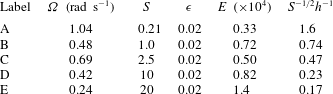
The key dimensionless parameters for each experiment are the Burger (
 $S$
), Ekman (
 $E$
) and Rossby (
 $\unicode[STIX]{x1D716}$
) numbers, defined here as
 $$\begin{eqnarray}\displaystyle S=\left(\frac{N}{\unicode[STIX]{x1D6FA}}\right)^{2},\quad E=\frac{\unicode[STIX]{x1D708}}{\unicode[STIX]{x1D6FA}L^{2}},\quad \unicode[STIX]{x1D716}=\frac{\unicode[STIX]{x0394}\unicode[STIX]{x1D6FA}}{\unicode[STIX]{x1D6FA}}. & & \displaystyle\end{eqnarray}$$
For the range of salinities used, the corresponding Schmidt number was
 $Sc\approx 670$
(Munro, Foster & Davies Reference Munro, Foster and Davies2010) and so molecular diffusion of salinity was negligible. The aspect ratio
 $h=H/L$
was throughout fixed at
 $h=1.35$
. Here we present results from five experiments. In all cases, the Ekman number was small with
 $E=O(10^{-4})$
, or less. Under these conditions, the structure and decay rate of the Rossby waves was determined by the magnitude of the Burger number, which was varied between
 $S=0.21$
and
 $S=20$
, by changing
 $\unicode[STIX]{x1D6FA}$
(as outlined in table 1) but also by changing
 $N$
. The Rossby number was kept fixed at
 $\unicode[STIX]{x1D716}=0.02$
; this is as small as the system would allow for the larger values of
 $S$
considered here. Table 1 lists the key parameters for the five experiments reported here, which are henceforth labelled A–E. We note that the values of angular frequency given in table 1 are those set via the digital drive used to control the turntable’s motor. The set angular frequency (both initial and final) was always verified by taking several independent measurements of the rotation period; the difference between the measured and set values of angular frequency was small and always less than 0.1 %.
The key parameters for the experiments, where
 $S=(N/\unicode[STIX]{x1D6FA})^{2}$
,
 $\unicode[STIX]{x1D716}=\unicode[STIX]{x0394}\unicode[STIX]{x1D6FA}/\unicode[STIX]{x1D6FA}$
and
 $E=\unicode[STIX]{x1D708}/\unicode[STIX]{x1D6FA}L^{2}$
. Also given are values of the vertical length scale
 $S^{-1/2}L$
, normalized by the container’s mean depth
 $H$
(namely,
 $S^{-1/2}h^{-1}$
).

van de Konijnenberg et al. (Reference van de Konijnenberg, Naulin, Rasmussen, Stenum and van Heijst2000) reported a series of experiments on the spin-up of a homogenous fluid in a sliced circular cylinder, and highlighted how the observed flow was dependent on the comparative magnitudes of the Rossby number (
 $\unicode[STIX]{x1D716}$
) and the base slope (
 $\unicode[STIX]{x1D6FC}$
). That is, in experiments performed with
 $\unicode[STIX]{x1D716}/\unicode[STIX]{x1D6FC}\geqslant O(1)$
the flow was dominated by the nonlinear separation of the sidewall boundary layer and subsequent shedding of cyclonic vorticity into the interior region. However, an experiment performed with
 $\unicode[STIX]{x1D716}/\unicode[STIX]{x1D6FC}\approx 0.04$
– corresponding to when the time scale associated with the formation of Rossby waves is small compared to the time scale associated with vortex shedding – showed clear evidence of Rossby-wave formation, with measurements in good agreement with the analytical results of Pedlosky & Greenspan (Reference Pedlosky and Greenspan1967). Therefore, in an effort to limit the effects associated with sidewall separation, we have
 $\unicode[STIX]{x1D716}/\unicode[STIX]{x1D6FC}\approx 0.1$
in all experiments reported here.
The flow was visualized and measured using particle image velocimetry (PIV). To facilitate the use of this technique, small tracer particles were suspended within the fluid column, which were added as the cylinder was filled and allowed to settle freely into suspension. A table-mounted light box was used to project a narrow light sheet through the cylinder’s sidewall to illuminate the tracer particles within a horizontal plane at a height
 $z_{0}^{\ast }$
above the centre of the base slope (see figure 1). The experiments listed in table 1 were first performed with
 $z_{0}^{\ast }=10~\text{cm}\approx 0.4H$
. So that the key height-dependent features of the flow could be identified, each experiment was then repeated, under near-identical conditions, with
 $z_{0}^{\ast }=5~\text{cm}\approx 0.2H$
(note that the top level of the base slope corresponds to height
 $0.14H$
). We were unable to take measurements at heights below
 $0.2H$
due to optical effects caused by the light sheet illuminating tracer particles that had settled onto the slope’s surface.
A co-rotating digital camera was mounted on the turntable and positioned to point vertically down into the cylinder’s interior (see figure 1), and used to record the particle motion within the illuminated horizontal plane, in the frame of reference that rotates with the turntable. The images were recorded at a frame rate of 10 Hz (at
 $1280\times 1024$
pixel resolution) and processed at the end of the experiment in terms of the co-rotating coordinates
 $(x^{\ast },y^{\ast },z^{\ast })$
, which are defined relative to the centre of the base plane, as shown in figure 1. The surface of the base plane is defined by
 $z^{\ast }=x^{\ast }\tan \unicode[STIX]{x1D6FC}$
. To relate these coordinates to the standard
 $\unicode[STIX]{x1D6FD}$
-plane convention (for anticlockwise rotation), we shall also refer to the up-slope
 $x$
-direction as north, and the long-slope
 $y$
-direction as west (see figure 1). Measurements of the horizontal velocity components
 $(u^{\ast },v^{\ast })$
and vertical vorticity field
 $\unicode[STIX]{x1D714}^{\ast }=v_{x^{\ast }}^{\ast }-u_{y^{\ast }}^{\ast }$
, in the illuminated plane at
 $z^{\ast }=z_{0}^{\ast }$
, were obtained by applying a standard PIV algorithm to the images (Dalziel Reference Dalziel2006). The PIV calculations were performed on consecutive images using square interrogation windows of
 $13\times 13$
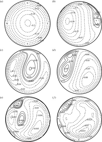
pixels, with an 8-pixel spacing overlap, which corresponds to a physical spacing between velocity vectors of approximately 0.04 cm and a temporal resolution of 0.1 s. The corresponding streamfunction was calculated from the measured vorticity field using a Poisson solver. We used a SLOR (successive line over-relaxation) method for the computations. In the remainder of this section we will use contours of the measured streamfunction to describe the key features of the observed flows; typical examples of these streamlines are shown in figure 2 (see caption for details).
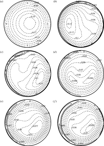
Streamlines from experiment A (
 $\unicode[STIX]{x1D6FA}=1.04~\text{rad}~\text{s}^{-1}$
,
 $S=0.21$
,
 $\unicode[STIX]{x1D716}=0.020$
), measured at the near mid-height
 $z_{0}^{\ast }=10~\text{cm}\approx 0.4H$
. The dimensionless times
 $\unicode[STIX]{x1D6FC}\unicode[STIX]{x1D6FA}t^{\ast }$
at which the data were taken are (a) 0.18, (b) 3.2, (c) 6.8, (d) 12, (e) 24 and (f) 45. The top (north) and bottom (south) of the base slope have been indicated in (a). The streamfunction values shown on each contour are dimensionless, and have been scaled by
 $\unicode[STIX]{x1D716}\unicode[STIX]{x1D6FA}L^{2}$
.

2.2 Observations
We have already noted that homogeneous spin-up in a sliced cylinder differs greatly from spin-up in a regular cylinder (
 $\unicode[STIX]{x1D6FC}=0$
), which is a gradual decay of the axisymmetric initial condition on the time scale
 $E^{-1/2}\unicode[STIX]{x1D6FA}^{-1}$
(Greenspan & Howard Reference Greenspan and Howard1963). In the sliced-cylinder configuration, the vortex lines of the initial condition when advected down the slope are stretched, producing vorticity relative to the rotating reference frame. The result is the formation, on the
 $\unicode[STIX]{x1D6FC}^{-1}\unicode[STIX]{x1D6FA}^{-1}$
time scale, of alternating cyclonic and anticyclonic vorticity waves that propagate across the slope; these two-dimensional vorticity waves gradually fill the fluid’s interior and are the primary mechanism resulting in the fluid’s spin-up. Pedlosky & Greenspan (Reference Pedlosky and Greenspan1967) described these vorticity waves theoretically for the case
 $\unicode[STIX]{x1D716}=0$
– showing they are a combination of all excited Rossby modes – and van de Konijnenberg et al. (Reference van de Konijnenberg, Naulin, Rasmussen, Stenum and van Heijst2000) reported observations and measurements from an experiment with
 $\unicode[STIX]{x1D716}=0.01$
,
 $\unicode[STIX]{x1D6FC}=0.244~\text{rad}$
(
 $14^{\circ }$
) which were in good agreement with the theory.
Here we describe how the observed flow differs when the fluid’s density field is linearly stratified, over the range of Burger number (
 $S$
) listed in table 1 and for
 $\unicode[STIX]{x1D716}=0.02$
,
 $\unicode[STIX]{x1D6FC}=0.175~\text{rad}$
(
 $10^{\circ }$
). Under these conditions the key experimental observations can be summarised as follows. At small
 $S$
the flow is very similar to that observed in the homogeneous case, with spin-up accomplished as two-dimensional, alternating vorticity waves fill the fluid’s interior. For
 $S\approx 1$
or greater, the strength of the fluid’s vertical density gradient is now sufficient to inhibit vortex stretching. As a result, the vorticity waves that form have a three-dimensional structure and are confined to a layer above the slope, the height of which decreases with increasing
 $S$
. The vorticity waves are also damped more rapidly as
 $S$
is increased. Therefore, at increasingly large
 $S$
the slope-induced effects become confined to an increasingly shallower layer, with the bulk-interior flow above remaining largely unaffected by the presence of the slope. We now illustrate this description using the experimental data.
To begin we consider experiment A, corresponding to the case of a weak stratification (
 $S=0.21$
). Figure 2 shows streamline data from experiment A, taken at the near mid-height
 $z_{0}^{\ast }=10~\text{cm}\approx 0.4H$
and at times ranging from the start of the experiment through to when the fluid is practically spun-up. The streamlines show the structure of the alternating vorticity waves as they propagate across the slope. To aid the reader in differentiating between the cyclonic and anticyclonic vorticity waves, we have shown negative streamlines as broken lines (anticyclonic flow) and positive streamlines as solid lines (cyclonic flow). For the configuration used here – with anticlockwise background rotation and north corresponding to the top of the slope – the vorticity waves appear first in the east side of the container and propagate westwards across the slope. We also note that the data obtained under these conditions at the near-slope height
 $z_{0}^{\ast }=5~\text{cm}\approx 0.2H$
were little different from the data shown in figure 2 (and so are not shown here). The key point here being that at small-
 $S$
the flow remained primarily two-dimensional throughout, in agreement with observations previously reported for the homogeneous case (van de Konijnenberg et al.
Reference van de Konijnenberg, Naulin, Rasmussen, Stenum and van Heijst2000).
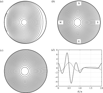
Immediately after the start of the experiment, the flow was an axisymmetric, anticyclonic vortex of the form shown in figure 2(a). The first vorticity wave (which has cyclonic circulation) can be seen forming adjacent to the eastern sidewall in figure 2(b), as the axis of the initial anticyclone moved across the slope into the western half of the domain. The first vorticity wave is shown at a later time in figure 2(c) as it proceeds across the container’s slope towards the western sidewall. In figure 2(b,c) there is a noticeable north–south asymmetry to the flow, evident by the structure of cyclonic vorticity wave being not fully extended north–south across the container. This asymmetry was also evident, to a similar degree, in the data obtained at the near-slope height
 $z^{\ast }=0.2H$
. The vorticity waves continue to form at subsequent times, entering from the east and propagating westwards, each with opposite-sense circulation to the previous one. For example, figures 2(d) and 2(e) show, respectively, the ‘second’ and ‘fourth’ vorticity waves shortly after formation, occupying the eastern half of the container, both with anticyclonic circulation and both preceded by a cyclonic vorticity wave (i.e. the ‘first’ and ‘third’ waves). As time increases, more and more vorticity waves fill the domain and the flow approaches a near spun-up state. It is known for the homogeneous case that viscous corrections due to the top and bottom Ekman layers lead to decay of the form
 $\exp [-2(E^{1/2}/h)\unicode[STIX]{x1D6FA}t^{\ast }]$
(Pedlosky & Greenspan Reference Pedlosky and Greenspan1967). The corresponding spin-up time scale for experiment A is equivalent to
 $\unicode[STIX]{x1D6FC}\unicode[STIX]{x1D6FA}t^{\ast }\approx 14$
, and so we expect the effects of Ekman suction to start becoming significant for times of the order or greater than this. There was no evidence of vorticity waves forming at times
 $\unicode[STIX]{x1D6FC}\unicode[STIX]{x1D6FA}t^{\ast }\gtrsim 34$
, and thereafter the residual relative flow took the form of a weak, slowly decaying, asymmetric anticyclone, as shown in figure 2(f).
We also note the presence of the small cyclonic vortex in the northwest perimeter region in figure 2(d–f). This is not a vorticity wave but is the result of vortex shedding from the western sidewall boundary layer. The time scale for shedding is of the order
 $\unicode[STIX]{x1D716}^{-1}\unicode[STIX]{x1D6FA}^{-1}$
, which was chosen here to be large in comparison to the time scale on which the Rossby waves form, which is of the order
 $\unicode[STIX]{x1D6FC}^{-1}\unicode[STIX]{x1D6FA}^{-1}$
: specifically,
 $\unicode[STIX]{x1D6FC}/\unicode[STIX]{x1D716}\approx 9$
in all experiments, and so the onset time of shedding, if it occurs, corresponds to
 $\unicode[STIX]{x1D6FC}\unicode[STIX]{x1D6FA}t^{\ast }\approx 12$
(as is the case figure 2). Under these conditions the shed vortex has a limited effect on the flow, and little if any effect on the initial Rossby waves, which consist of the largest-scale modes. The key effect – evident in figure 2(d,e) – is that the formation and shedding of this vortex resulted in a slight increase in the degree of north–south asymmetry evident in the flow. We will discuss in more detail the shedding process in § 7.
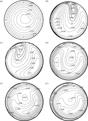
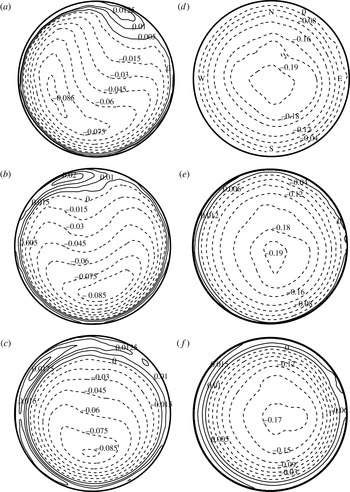
Streamlines from experiment B (
 $\unicode[STIX]{x1D6FA}=0.48~\text{rad}~\text{s}^{-1}$
,
 $S=1.0$
,
 $\unicode[STIX]{x1D716}=0.020$
), measured at the near-slope height
 $z_{0}^{\ast }=5~\text{cm}\approx 0.2H$
. The dimensionless times
 $\unicode[STIX]{x1D6FC}\unicode[STIX]{x1D6FA}t^{\ast }$
at which the data were taken are (a) 0.16, (b) 3.4, (c) 5.4, (d) 11, (e) 19 and (f) 37. The top (north) and bottom (south) of the base slope have been indicated in (a). The streamfunction values shown on each contour are dimensionless, and have been scaled by
 $\unicode[STIX]{x1D716}\unicode[STIX]{x1D6FA}L^{2}$
.

Streamlines from experiment B (
 $\unicode[STIX]{x1D6FA}=0.48~\text{rad}~\text{s}^{-1}$
,
 $S=1.0$
,
 $\unicode[STIX]{x1D716}=0.020$
), measured at the near mid-height
 $z_{0}^{\ast }=10~\text{cm}\approx 0.4H$
. The dimensionless times
 $\unicode[STIX]{x1D6FC}\unicode[STIX]{x1D6FA}t^{\ast }$
at which the data were taken are (a) 0.16, (b) 3.4, (c) 5.4, (d) 11, (e) 19 and (f) 37. The top (north) and bottom (south) of the base slope have been indicated in (a). The streamfunction values shown on each contour are dimensionless, and have been scaled by
 $\unicode[STIX]{x1D716}\unicode[STIX]{x1D6FA}L^{2}$
.

For comparison, figures 3 and 4 show streamline data for
 $S=1.0$
(experiment B). Under these conditions – unlike the data just described – the flow had a clear height-dependent structure and so for this case we have shown data at both heights:
 $z_{0}^{\ast }=5~\text{cm}\approx 0.2H$
(figure 3) and
 $z_{0}^{\ast }=10~\text{cm}\approx 0.4H$
(figure 4). At early times, the starting flow was a two-dimensional, axisymmetric anticyclone, as shown in figures 3(a) and 4(a). At subsequent times, however, clear differences in the flow’s structure were evident at the two heights: consider first the near-slope data in figure 3 (taken at
 $z_{0}^{\ast }=0.2H$
), which clearly show the presence of alternating vorticity waves at this height. The first vorticity wave – which has cyclonic circulation (solid streamlines) – is shown shortly after forming in figure 3(b) and at a later time in figure 3(c), having moved westwards across the slope; again, this cyclonic wave is proceeded by the initial anticyclone and followed by the second vorticity wave, which has anticyclonic circulation. When compared with the small-
 $S$
data in figure 2, there are a number of key differences to highlight: (i) there is a greater degree of north–south asymmetry evident in the streamlines; in particular, the first vorticity wave, as it moved across the slope, remained confined to the northern half of the plane, while the second wave (anticyclonic) that followed remained positioned in the southern half of the plane, as shown in figure 3(b,c). (ii) Relative to the scaled time
 $\unicode[STIX]{x1D6FC}\unicode[STIX]{x1D6FA}t^{\ast }$
, the vorticity waves formed earlier and travelled more rapidly across the slope; this can be seen by comparing figure 3(b) with figure 2(b), which both correspond to
 $\unicode[STIX]{x1D6FC}\unicode[STIX]{x1D6FA}t^{\ast }=3.4$
. (iii) Figure 3(c) shows the first vorticity wave (cyclonic) approaching the north-west region of the sidewall; upon reaching the sidewall, this vortex remained positioned within the western-sidewall region, which appeared to preclude the development of large adverse pressure gradients in this region. As a result, there was no vortex shedding and subsequent formation of a persistent cyclonic vortex adjacent to the north-west sidewall region (as was the case in figure 2). (iv) Vorticity waves were seen to form at times subsequent to this, however, only waves with anticyclonic circulation. For example, figure 3(d) shows the second vorticity wave (anticyclonic) as it approaches the western sidewall, followed by another anticyclonic wave located near the central axis of the cylinder. (v) There was no formation of vorticity waves for times
 $\unicode[STIX]{x1D6FC}\unicode[STIX]{x1D6FA}t^{\ast }\gtrsim 14$
, indicating that at this larger value of
 $S$
the Rossby modes were damped more rapidly. At times subsequent to this the measured streamlines took the form of the quasi-steady, asymmetric anticyclone shown in figure 3(e,f), which thereafter decayed gradually.
Streamline data at corresponding times, but taken at the near mid-depth
 $z_{0}^{\ast }=0.4H$
, are shown in figure 4. Again, the starting-flow anticyclone, once formed, moved westwards across the slope (see figure 4
b), although, there was no following cyclonic vortex wave present within the bulk interior at this height. However, we draw attention to the thin region of cyclonic vorticity in figure 4(b), which at this time is positioned adjacent to the north-north-east region of the sidewall, which subsequently moved westwards across the slope, but throughout remained confined within a narrow region close to the sidewall – for example, figure 4(c) shows this cyclonic vortex at a later time positioned adjacent to the sidewall, at north-west. Moreover, the westward trajectory of this near-wall vortex coincides with the trajectory of the first vorticity wave evident at height
 $z^{\ast }=0.2H$
; this can be seen by comparing figure 4(b,c) with figure 3(b,c). (We note that this vortex is not a result of shedding at the north-west sidewall, as shedding would occur at a later time,
 $\unicode[STIX]{x1D6FC}\unicode[STIX]{x1D6FA}t^{\ast }\approx 12$
.) It appears, therefore, that under these conditions the cyclonic vortex has a three-dimensional structure, becoming ‘thinner’ and increasingly more confined closer to the sidewall as height above the slope is increased. On reaching the western sidewall region, the cyclonic vortex remained there. There was again evidence of vorticity waves forming at this height at later times, but as was the case at the near-slope height (figure 3), only waves with anticyclonic circulation – for example, see figure 4(c,d). No waves were seen to form for times
 $\unicode[STIX]{x1D6FC}\unicode[STIX]{x1D6FA}t^{\ast }\gtrsim 14$
, and thereafter the flow took the form of a quasi-steady, asymmetric anticyclone which decayed slowly, as shown in figure 4(e,f).
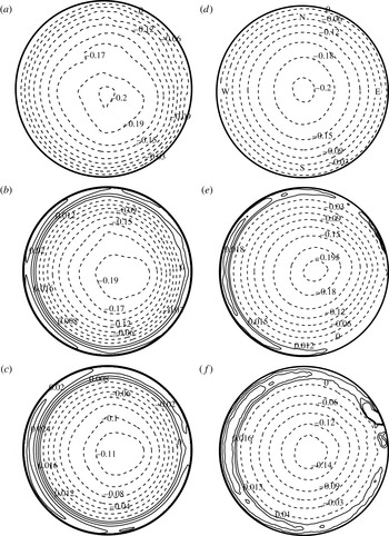
Streamlines from experiment D (
 $\unicode[STIX]{x1D6FA}=0.42~\text{rad}~\text{s}^{-1}$
,
 $S=10$
,
 $\unicode[STIX]{x1D716}=0.020$
). The data in (a–c), were measured at the near-slope height
 $z_{0}^{\ast }=5~\text{cm}\approx 0.2H$
; the data in (d–f), were measured at the near-mid-height
 $z_{0}^{\ast }=10~\text{cm}\approx 0.4H$
. The dimensionless times
 $\unicode[STIX]{x1D6FC}\unicode[STIX]{x1D6FA}t^{\ast }$
at which the data were taken are (a,d) 1.1, (b,e) 2.0 and (c,f) 18. The top (north) and bottom (south) of the base slope are shown in (d). The streamfunction values shown on each contour are dimensionless, and have been scaled by
 $\unicode[STIX]{x1D716}\unicode[STIX]{x1D6FA}L^{2}$
.

The streamline data from experiment C (
 $S=2.5$
) are qualitatively very similar to the data shown in figures 3 and 4 for
 $S=1$
, and so are not shown here. However, at
 $S=2.5$
we did note a comparative increase in the degree of north–south asymmetry evident in the first vorticity wave (cyclonic) at the height
 $z_{0}^{\ast }\approx 0.2H$
– it being confined even further north in the plane – and that no vorticity waves were seen to form for times
 $\unicode[STIX]{x1D6FC}\unicode[STIX]{x1D6FA}t^{\ast }\gtrsim 9$
.
The effects of further increasing
 $S$
can be seen in figure 5, which shows data for
 $S=10$
(experiment D). Comparatively fewer features were evident in these data and so the figure is formatted with the left-hand column showing streamlines measured at the near-slope height (
 $z_{0}^{\ast }=5~\text{cm}\approx 0.2H$
), and the right-hand column showing data measured at the near mid-height (
 $z_{0}^{\ast }=10~\text{cm}\approx 0.4H$
). See figure captions for details. Consider first the data at the near-slope height: unlike the data already presented, the initial anticyclone at this height was north–south asymmetric from the outset, forming with its centre located in the southern half of the plane. Once formed, the anticyclone quickly moved westwards, as shown in figure 5(a), and the first cyclonic vortex wave formed adjacent to the north-east region of the sidewall, which subsequently moved westwards around the northern sidewall of the container (as shown in figure 5
b). Comparing these streamlines with those in figure 3 (also taken at
 $z_{0}^{\ast }\approx 0.2H$
, but for
 $S=1$
) confirms that further increasing the relative strength of the stratification resulted in a more rapid formation (and propagation) of the cyclonic vorticity wave, relative to the scaled time
 $\unicode[STIX]{x1D6FC}\unicode[STIX]{x1D6FA}t^{\ast }$
, and with the wave at this height being further confined within a region close to the northern sidewall (i.e. an increased north–south asymmetry). In addition, at this larger value of
 $S$
the Rossby modes were damped more rapidly; as a result, following the formation of the first wave, no vorticity waves were seen to form at this height, at subsequent times. Instead, the interior core region throughout remained occupied by the initial anticyclone, whose core moved from its displaced western position back into the southern half of the domain as the cyclonic vortex wave moved around the northern sidewall, as shown by comparing figure 5(a,b). Shortly after this, the cyclonic vortex entered the western boundary region where it remained, and thereafter the flow took the form of a quasi-steady, asymmetric anticyclone which decayed slowly. Figure 5(c) shows streamlines at a much later time, which have not changed significantly in comparison with those shown in figure 5(b). We also stress that the cyclonic vortex evident in the north-west sidewall region of figure 5(c) is the remnant of the first vorticity wave and is not a result of shedding from the western-sidewall region.
In contrast, the streamline data in figure 5(d–f), taken at corresponding times but at
 $z_{0}^{\ast }\approx 0.4H$
, show that from the outset, and throughout the period shown, the flow at the near mid-height took the form of a slowly decaying, near-axisymmetric anticyclone. Slight irregularities were evident in the streamlines about the cylinder’s axis, but the outer streamlines remained near circular throughout. Notably, none of the slope-induced flow features described above were observed in the data, and so the flow at this height appears to have been little affected by the presence of the slope. The slope-induced features were certainly confined within a layer above the slope of height less than
 $0.4H$
.
Further evidence to confirm this bottom trapping of slope-induced features is shown in figure 6, which shows streamline data from our extreme case
 $S=20$
(experiment E). Again, given the comparative featureless nature of these data, the figure is formatted with the data in the left-hand and right-hand columns taken, respectively, at
 $z_{0}^{\ast }\approx 0.2H$
and
 $z_{0}^{\ast }\approx 0.4H$
. In this case, at both heights, the flow had the form of slowly decaying, axisymmetric anticyclone, although at the near-slope height the streamlines did exhibit slight but noticeable irregularities (similar to those observed at the near mid-height in figure 5). These data clearly show that any flow features induced by the presence of the slope must have been confined to heights
 $z^{\ast }<0.2H$
. There are certainly no Rossby waves evident in these data. (We have already noted that we were unable to take measurements at heights much below
 $z^{\ast }=0.2H$
, due to optical effects caused by the light sheet illuminating tracer particles that had settled onto the slope’s surface. Recall, the top level of the base slope corresponds to
 $z^{\ast }=0.14H$
.)
The theory presented in § 6 below shows that as
 $S$
gets large the stratified Rossby waves become increasingly confined to a layer of height of the order
 $S^{-1/2}L$
above the mid-slope. We have therefore included in table 1 the corresponding height scales for each experiment, normalized by the container’s mean depth
 $H$
(namely,
 $S^{-1/2}h^{-1}$
). Comparing these scales with the experimental observations shows a good qualitative confirmation for the presence of the layer. That is, for experiments A, B and C we have
 $S^{-1/2}h^{-1}\geqslant 0.47$
and in each of these cases the Rossby waves were observed at both of the sample heights
 $z^{\ast }/H=0.2$
and 0.4. In contrast,
 $S^{-1/2}h^{-1}=0.23$
in experiment D and the Rossby waves were observed only at
 $z^{\ast }/H=0.2$
, but not at
 $z^{\ast }/H=0.4$
. Under the more extreme conditions of experiment E, with
 $S^{-1/2}h^{-1}=0.17$
, no Rossby waves were observed at either of the sample heights.
Streamlines from experiment E (
 $\unicode[STIX]{x1D6FA}=0.24~\text{rad}~\text{s}^{-1}$
,
 $S=20$
,
 $\unicode[STIX]{x1D716}=0.020$
). The data in (a–c), were measured at the near-slope height
 $z_{0}^{\ast }=5~\text{cm}\approx 0.2H$
; the data in (d–f), were measured at the near-mid-height
 $z_{0}^{\ast }=10~\text{cm}\approx 0.4H$
. The dimensionless times
 $\unicode[STIX]{x1D6FC}\unicode[STIX]{x1D6FA}t^{\ast }$
at which the data were taken are (a,d) 0.27, (b,e) 10 and (c,f) 30. The top (north) and bottom (south) of the base slope are shown in (d). The streamfunction values shown on each contour are dimensionless, and have been scaled by
 $\unicode[STIX]{x1D716}\unicode[STIX]{x1D6FA}L^{2}$
.

3 Problem formulation
Following the approach used in Munro & Foster (Reference Munro and Foster2014), we scale time, lengths and velocities with
 $\unicode[STIX]{x1D6FA}^{-1}$
,
 $L$
and
 $\unicode[STIX]{x1D716}\unicode[STIX]{x1D6FA}L$
, and let
 $(r,\unicode[STIX]{x1D703},z)$
and
 $(u,v,w)$
denote the dimensionless polar coordinate directions and corresponding velocity components. The Navier–Stokes equations (with usual Boussinesq approximation), in the rotating reference frame of the final rotation rate, are given by
 $$\begin{eqnarray}\displaystyle & \displaystyle \unicode[STIX]{x1D735}\boldsymbol{\cdot }\boldsymbol{u}=0, & \displaystyle\end{eqnarray}$$
 $$\begin{eqnarray}\displaystyle & \displaystyle \boldsymbol{u}_{t}+\unicode[STIX]{x1D716}(\boldsymbol{u}\boldsymbol{\cdot }\unicode[STIX]{x1D735})\boldsymbol{u}+2\hat{\boldsymbol{z}}\times \boldsymbol{u}+\unicode[STIX]{x1D70C}\hat{\boldsymbol{z}}+\unicode[STIX]{x1D735}p=E\unicode[STIX]{x1D6FB}^{2}\boldsymbol{u}, & \displaystyle\end{eqnarray}$$
 $$\begin{eqnarray}\displaystyle & \displaystyle \unicode[STIX]{x1D70C}_{t}+\unicode[STIX]{x1D716}(\boldsymbol{u}\boldsymbol{\cdot }\unicode[STIX]{x1D735})\unicode[STIX]{x1D70C}-Sw=0, & \displaystyle\end{eqnarray}$$
 $\hat{\boldsymbol{z}}$
is the vertical unit vector, aligned with the axis of rotation and
 $\unicode[STIX]{x1D703}=0$
corresponds to the up-slope direction (i.e. north). The dimensionless Ekman number (
 $E$
), Burger number (
 $S$
) and Rossby number (
 $\unicode[STIX]{x1D716}$
) have been defined above in (2.1). The quantities
 $p(\boldsymbol{x},t)$
and
 $\unicode[STIX]{x1D70C}(\boldsymbol{x},t)$
in (3.1) denote perturbations in pressure and density about the initial state of solid rotation, which have been scaled with
 $\unicode[STIX]{x1D716}\unicode[STIX]{x1D70C}_{H}\unicode[STIX]{x1D6FA}^{2}L^{2}$
and
 $\unicode[STIX]{x1D716}\unicode[STIX]{x1D70C}_{H}\unicode[STIX]{x1D6FA}^{2}L/g$
, respectively, where
 $\unicode[STIX]{x1D70C}_{H}$
is a constant reference density, here taken as the fluid’s initial density at the lid. We have ignored the finite diffusivity of salt in water – essentially an infinite Schmidt number approximation. The initial and boundary conditions are given by
 $$\begin{eqnarray}\displaystyle \boldsymbol{u}=\boldsymbol{x}\times \hat{\boldsymbol{z}}=(0,-r,0),\quad \unicode[STIX]{x1D70C}=0,\quad \text{for}\;t=0\;\text{and}\;\boldsymbol{x}\in \mathscr{D}, & & \displaystyle\end{eqnarray}$$
 $$\begin{eqnarray}\displaystyle \boldsymbol{u}=\mathbf{0},\quad \frac{\unicode[STIX]{x2202}\unicode[STIX]{x1D70C}}{\unicode[STIX]{x2202}n}=0,\quad \text{for}\;\boldsymbol{x}\in \unicode[STIX]{x2202}\mathscr{D}, & & \displaystyle\end{eqnarray}$$
where
 $\mathscr{D}$
is the solution domain, defined as
 $$\begin{eqnarray}\displaystyle \mathscr{D}=\{(r,\unicode[STIX]{x1D703},z):r\in [0,1],\unicode[STIX]{x1D703}\in [0,2\unicode[STIX]{x03C0}),z\in [\unicode[STIX]{x1D6FC}r\cos \unicode[STIX]{x1D703},h]\}, & & \displaystyle\end{eqnarray}$$
and
 $\unicode[STIX]{x2202}\mathscr{D}$
is the boundary of
 $\mathscr{D}$
. Recall that
 $h=H/L$
.
Our approach here is to use asymptotic methods for
 $\unicode[STIX]{x1D716},E\rightarrow 0$
, in that order – hence, nonlinearity is neglected throughout the analytical treatment here. It is well known, on time scales much larger than order one, that away from thin boundary layers, the motion is governed by the elliptic equation (Munro & Foster Reference Munro and Foster2014)
 $$\begin{eqnarray}\displaystyle \unicode[STIX]{x1D6FB}_{1}^{2}p+\frac{4}{S}p_{zz}=-4. & & \displaystyle\end{eqnarray}$$
Here,
 $\unicode[STIX]{x1D6FB}_{1}^{2}=\unicode[STIX]{x2202}^{2}/\unicode[STIX]{x2202}r^{2}+r^{-1}\unicode[STIX]{x2202}/\unicode[STIX]{x2202}r+r^{-2}\unicode[STIX]{x2202}^{2}/\unicode[STIX]{x2202}\unicode[STIX]{x1D703}^{2}$
is the horizontal Laplacian, and the velocity components are obtained from the pressure by
 $$\begin{eqnarray}\displaystyle u=-\frac{p_{\unicode[STIX]{x1D703}}}{2r},\quad v=\frac{p_{r}}{2},\quad w=-\frac{p_{zt}}{S}. & & \displaystyle\end{eqnarray}$$
The lower (sloped) surface is given by
 $z=\unicode[STIX]{x1D6FC}x$
, with
 $\unicode[STIX]{x1D6FC}\ll 1$
as noted above. Then, the boundary condition at the lower wall is
 $$\begin{eqnarray}\displaystyle p_{zt}=\frac{\unicode[STIX]{x1D6FC}S}{2}\left(p_{r}\sin \unicode[STIX]{x1D703}+p_{\unicode[STIX]{x1D703}}\frac{\cos \unicode[STIX]{x1D703}}{r}\right)~\text{on}~z=0, & & \displaystyle\end{eqnarray}$$
where the boundary condition has been transferred to
 $z=0$
in the usual way; the upper-wall boundary condition is given by
 $p_{zt}=0$
. However, the velocity normal to the upper and lower walls is not zero, since the presence of Ekman layers on both walls – neglected to arrive at (3.4) – cause inflow or outflow into the core. Thus, the lower- and upper-surface boundary conditions – including ‘Ekman suction’ – become
 $$\begin{eqnarray}\displaystyle p_{z\unicode[STIX]{x1D70F}}=\frac{S}{2}\left(p_{r}\sin \unicode[STIX]{x1D703}+p_{\unicode[STIX]{x1D703}}\frac{\cos \unicode[STIX]{x1D703}}{r}\right)-\unicode[STIX]{x1D702}\frac{S}{4}\unicode[STIX]{x1D6FB}_{1}^{2}p+\mathscr{E}_{0}\quad \text{on}~z=0, & & \displaystyle\end{eqnarray}$$
and
 $$\begin{eqnarray}\displaystyle p_{z\unicode[STIX]{x1D70F}}=\unicode[STIX]{x1D702}\frac{S}{4}\unicode[STIX]{x1D6FB}_{1}^{2}p+\mathscr{E}_{h}\quad \text{on}~z=h, & & \displaystyle\end{eqnarray}$$
where
 $$\begin{eqnarray}\displaystyle \unicode[STIX]{x1D70F}=\unicode[STIX]{x1D6FC}t,\quad \unicode[STIX]{x1D702}=E^{1/2}/\unicode[STIX]{x1D6FC}. & & \displaystyle\end{eqnarray}$$
The transferring of the boundary condition from
 $z=\unicode[STIX]{x1D6FC}x$
to
 $z=0$
leads to order-
 $\unicode[STIX]{x1D6FC}$
corrections to (3.7a
), leading to an upper ordering on
 $\unicode[STIX]{x1D6FC}\ll E^{1/4}$
, so this asymptotic theory requires that
 $$\begin{eqnarray}\displaystyle E^{1/2}\ll \unicode[STIX]{x1D6FC}\ll E^{1/4}. & & \displaystyle\end{eqnarray}$$
A quantity
 $\mathscr{E}$
has been appended to (3.7), however. We have discussed elsewhere (Foster & Munro Reference Foster and Munro2012; Munro & Foster Reference Munro and Foster2014) that in these non-axisymmetric flows, the Ekman layers are not empty of fluid, where the upper and lower walls intersect the vertical cylinder wall, and so fluid erupts into the interior at those junctions. The source/sink strength,
 $\mathscr{E}$
– non-zero only at
 $r=1$
– must be chosen such that the net-vertical momentum flux at both upper and lower boundaries is zero. That is, all fluid that enters the Ekman layer along its length must erupt into the interior at the edge of the disk; there is no mechanism in these flows for order-one vertical momentum transport in the interior, or in a sidewall layer – as there would be in the homogeneous case.
This no-net-vertical transport constraint means that the solution to (3.4) must be such that
 $$\begin{eqnarray}\displaystyle \int _{0}^{1}\int _{0}^{2\unicode[STIX]{x03C0}}p_{z\unicode[STIX]{x1D70F}}r\,\text{d}r\,\text{d}\unicode[STIX]{x1D703}=0\quad \text{at}~z=0,h. & & \displaystyle\end{eqnarray}$$
Before moving on to the mathematical results and comparison with experiment, we note an obvious fact that this problem, as formulated in (3.4), (3.7a
) and (3.7b
), is invariant under the transformation
 $x\rightarrow (-x)$
, so that all solutions will be symmetric around the
 $y$
axis. In terms of the discussion in the previous section, the theory always gives north–south symmetry. Therefore, any north–south asymmetry arises from some effects not contained in this theory – see the discussion in § 7.
4 Small-
 $S$
case

Following the approach used in section IV of Munro & Foster (Reference Munro and Foster2014), we found for
 $S=0$
that the leading-order term in an asymptotic series in
 $S$
is
 $$\begin{eqnarray}\displaystyle p_{0}=\mathscr{G}(r,\unicode[STIX]{x1D703},\unicode[STIX]{x1D70F})\text{e}^{-2\unicode[STIX]{x1D702}\unicode[STIX]{x1D70F}/h}, & & \displaystyle\end{eqnarray}$$
and
 $\mathscr{G}$
obeys the equation
 $$\begin{eqnarray}\displaystyle \frac{h}{2}\unicode[STIX]{x1D6FB}_{1}^{2}\mathscr{G}_{\unicode[STIX]{x1D70F}}=\mathscr{G}_{y}. & & \displaystyle\end{eqnarray}$$
Pedlosky & Greenspan (Reference Pedlosky and Greenspan1967) make a substitution
 $$\begin{eqnarray}\displaystyle \mathscr{G}=F(r,\unicode[STIX]{x1D703})\text{e}^{\unicode[STIX]{x1D6FC}\unicode[STIX]{x1D70F}+\unicode[STIX]{x1D6FD}y}, & & \displaystyle\end{eqnarray}$$
leading to
 $$\begin{eqnarray}\displaystyle \unicode[STIX]{x1D6FB}_{1}^{2}F-\unicode[STIX]{x1D6FD}^{2}F=0, & & \displaystyle\end{eqnarray}$$
if one makes the choice
 $\unicode[STIX]{x1D6FC}\unicode[STIX]{x1D6FD}h=1$
. No penetration at the sidewalls means the solution may be written as
 $$\begin{eqnarray}\displaystyle \mathscr{G}=\mathop{\sum }_{m=1}^{\infty }\mathop{\sum }_{n=0}^{\infty }a_{mn}J_{n}(\unicode[STIX]{x1D6FC}_{mn}r)\text{e}^{\text{i}n\unicode[STIX]{x1D703}}\text{e}^{\text{i}\unicode[STIX]{x1D6FC}_{mn}y-\text{i}\unicode[STIX]{x1D70F}/(h\unicode[STIX]{x1D6FC}_{mn})}, & & \displaystyle\end{eqnarray}$$
where
 $\unicode[STIX]{x1D6FC}_{mn}$
is the
 $m$
th zero of
 $J_{n}(r)$
. Hence, we have the complete, leading-order solution (4.1). There is a common intuition about wave propagation problems that large-wavenumber waves are more strongly damped, but we note that is not so here – all of the damping coefficients are identical and so not dependent on wavenumber.
5 General case:
$S=O(1)$

We now expand the solution in the interior as an asymptotic series,
 $$\begin{eqnarray}\displaystyle p(\boldsymbol{x},\unicode[STIX]{x1D70F})=p_{0}(\boldsymbol{x},\unicode[STIX]{x1D70F})+\unicode[STIX]{x1D702}p_{1}(\boldsymbol{x},\unicode[STIX]{x1D70F})+\cdots \,, & & \displaystyle\end{eqnarray}$$
and substitute into the pressure equation, with the time suitably scaled. The result for the first-order problem is, from (3.4)
 $$\begin{eqnarray}\displaystyle \unicode[STIX]{x1D6FB}_{1}^{2}p_{0}+\frac{4}{S}p_{0zz}=-4, & & \displaystyle\end{eqnarray}$$
subject to no penetration at the vertical walls – that is,
 $p_{0}=0$
on
 $r=1$
.
In a fashion analogous to the analysis used for the sliced square cylinder (Munro & Foster Reference Munro and Foster2014), we take the ansatz to be
 $$\begin{eqnarray}\displaystyle p_{0} & = & \displaystyle \mathop{\sum }_{n=0}^{\infty }\mathop{\sum }_{m=1}^{\infty }A_{mn}(z,\unicode[STIX]{x1D70F})\cos (n\unicode[STIX]{x1D703})J_{n}(\unicode[STIX]{x1D6FC}_{mn}r)+\mathop{\sum }_{n=1}^{\infty }\mathop{\sum }_{m=1}^{\infty }B_{mn}(z,\unicode[STIX]{x1D70F})\sin (n\unicode[STIX]{x1D703})J_{n}(\unicode[STIX]{x1D6FC}_{mn}r)\nonumber\\ \displaystyle & & \displaystyle +\,K_{1}(r,\unicode[STIX]{x1D703},\unicode[STIX]{x1D70F})+zK_{2}(\unicode[STIX]{x1D70F})+z^{2}K_{3}(\unicode[STIX]{x1D70F}),\end{eqnarray}$$
where
 $\{\unicode[STIX]{x1D6FC}_{mn}\}$
constitutes all of the zeros of
 $J_{n}(r)$
, with counting starting at
 $m=1$
. Before examining the equations for
 $A_{mn}$
and
 $B_{mn}$
, we note that
 $$\begin{eqnarray}\displaystyle \unicode[STIX]{x1D6FB}_{1}^{2}K_{1}=-\frac{8}{S}\,K_{3}, & & \displaystyle\end{eqnarray}$$
and its solution is simply
 $$\begin{eqnarray}\displaystyle K_{1}=\frac{2K_{3}}{S}(1-r^{2}). & & \displaystyle\end{eqnarray}$$
Substitution into (5.2) leads to the solutions for Fourier–Bessel coefficients,
 $$\begin{eqnarray}\displaystyle & \displaystyle A_{m0}=\frac{c_{m}}{\unicode[STIX]{x1D6FC}_{m0}^{2}}+a_{m0}\cosh [\unicode[STIX]{x1D707}_{m0}(z-h)]+e_{m0}\sinh [\unicode[STIX]{x1D707}_{m0}(z-h)],\quad m=1,2,3,\ldots & \displaystyle\end{eqnarray}$$
 $$\begin{eqnarray}\displaystyle & \displaystyle A_{mn}=a_{mn}\cosh [\unicode[STIX]{x1D707}_{mn}(z-h)]+e_{mn}\sinh [\unicode[STIX]{x1D707}_{mn}(z-h)],\quad m,n=1,2,3,\ldots & \displaystyle\end{eqnarray}$$
 $$\begin{eqnarray}\displaystyle & \displaystyle B_{mn}=b_{mn}\cosh [\unicode[STIX]{x1D707}_{m0}(z-h)]+f_{mn}\sinh [\unicode[STIX]{x1D707}_{mn}(z-h)],\quad m,n=1,2,3,\ldots & \displaystyle\end{eqnarray}$$
 $$\begin{eqnarray}\displaystyle \unicode[STIX]{x1D707}_{mn}=\frac{\sqrt{S}}{2}\unicode[STIX]{x1D6FC}_{mn},\quad c_{m}=\frac{8}{\unicode[STIX]{x1D6FC}_{m0}J_{1}(\unicode[STIX]{x1D6FC}_{m0})}. & & \displaystyle\end{eqnarray}$$
Employing the vertical motion constraint (3.10) leads to equations for
 $K_{2}$
and
 $K_{3}$
, namely
 $$\begin{eqnarray}\displaystyle & \displaystyle \mathop{\sum }_{m=1}^{\infty }\frac{A_{m0,z\unicode[STIX]{x1D70F}}}{\unicode[STIX]{x1D6FC}_{m0}}J_{1}(\unicode[STIX]{x1D6FC}_{m0})+\frac{1}{2}K_{2,\unicode[STIX]{x1D70F}}=0,\quad \text{on}~z=0, & \displaystyle\end{eqnarray}$$
 $$\begin{eqnarray}\displaystyle & \displaystyle \mathop{\sum }_{m=1}^{\infty }\frac{A_{m0,z\unicode[STIX]{x1D70F}}}{\unicode[STIX]{x1D6FC}_{m0}}J_{1}(\unicode[STIX]{x1D6FC}_{m0})+\frac{1}{2}(K_{2,\unicode[STIX]{x1D70F}}+2hK_{3,\unicode[STIX]{x1D70F}})=0,\quad \text{on}~z=h, & \displaystyle\end{eqnarray}$$
 $K_{2}$
and
 $K_{3}$
, using the homogeneous initial conditions for
 $A_{mn},B_{mn}$
, are
 $$\begin{eqnarray}\displaystyle & \displaystyle K_{2}=-2\mathop{\sum }_{m=1}^{\infty }A_{m0,z}|_{z=0}\frac{J_{1}(\unicode[STIX]{x1D6FC}_{m0})}{\unicode[STIX]{x1D6FC}_{m0}}, & \displaystyle\end{eqnarray}$$
 $$\begin{eqnarray}\displaystyle & \displaystyle K_{3}=-\frac{1}{h}\mathop{\sum }_{m=1}^{\infty }(A_{m0,z}|_{z=h}-A_{m0,z}|_{z=0})\frac{J_{1}(\unicode[STIX]{x1D6FC}_{m0})}{\unicode[STIX]{x1D6FC}_{m0}}. & \displaystyle\end{eqnarray}$$
The overall procedure for such a solution follows precisely that given in Munro & Foster (Reference Munro and Foster2014) for a cylinder of square cross-section, and so for brevity, we choose not to give all of the details here; the circular geometry increases the algebraic complexity of the process. Those details have been relegated to appendix A. Because of the interesting interplay of Rossby waves and surface friction at large
 $S$
, we do include more details in the large-
 $S$
analysis in the next section of this paper.
5.1 The steady state
There are stratified Rossby waves in the container, and frictional decay. For
 $\unicode[STIX]{x1D702}\unicode[STIX]{x1D70F}\rightarrow \infty$
, the solution to the equations developed in appendix A takes a steady structure, and this structure erodes slowly on a viscous time scale. It is shown in appendix A that the steady solution is
 $$\begin{eqnarray}\displaystyle p_{0} & = & \displaystyle K_{3}\left[\frac{2}{S}(1-r^{2})+z^{2}-zh+\mathop{\sum }_{k=1}^{\infty }\frac{c_{k}}{2\unicode[STIX]{x1D707}_{k0}^{2}}\frac{\sinh [\unicode[STIX]{x1D707}_{k0}(z-h)]-\sinh (\unicode[STIX]{x1D707}_{k0}z)}{\sinh (\unicode[STIX]{x1D707}_{k0}h)}\;J_{0}(\unicode[STIX]{x1D6FC}_{k0}r)\right]\nonumber\\ \displaystyle & & \displaystyle -\,\mathop{\sum }_{k=1}^{\infty }\frac{c_{k}}{\unicode[STIX]{x1D6FC}_{k0}^{2}}\;\frac{\sinh (\unicode[STIX]{x1D707}_{k0}z)-\sinh [\unicode[STIX]{x1D707}_{k0}(z-h)]-\sinh (\unicode[STIX]{x1D707}_{k0}h)}{\sinh (\unicode[STIX]{x1D707}_{k0}h)}\;J_{0}(\unicode[STIX]{x1D6FC}_{k0}r),\end{eqnarray}$$
 $$\begin{eqnarray}\displaystyle K_{3}=-\frac{8\unicode[STIX]{x1D70E}\;S}{hS^{1/2}-16\unicode[STIX]{x1D70E}}, & & \displaystyle\end{eqnarray}$$
 $$\begin{eqnarray}\displaystyle \unicode[STIX]{x1D70E}\equiv \mathop{\sum }_{k=1}^{\infty }\frac{\cosh (\unicode[STIX]{x1D707}_{k0}h)-1}{\unicode[STIX]{x1D6FC}_{k0}^{3}\sinh (\unicode[STIX]{x1D707}_{k0}h)}. & & \displaystyle\end{eqnarray}$$
We now examine two extreme cases. First of all, for large
 $S$
, the
 $\unicode[STIX]{x1D70E}$
sum can be seen to be of order one, so from (5.8b
), we can see that
 $K_{3}=O(S^{1/2})$
. In (5.8a
), the square bracket terms multiplying
 $K_{3}$
are order
 $S^{-1}$
, so that term takes a limiting form that is of order
 $S^{-1/2}$
, and is hence small for large
 $S$
. The final term in (5.8a
) gives the dominant behaviour
 $$\begin{eqnarray}\displaystyle p_{0}\sim \mathop{\sum }_{k=1}^{\infty }\frac{c_{k}}{\unicode[STIX]{x1D6FC}_{k0}^{2}}\;J_{0}(\unicode[STIX]{x1D6FC}_{k0}r)=1-r^{2}+O(S^{1/2}),\quad \text{for }S\text{ large}. & & \displaystyle\end{eqnarray}$$
The same result is given in § 6.3.1 below for the large-
 $S$
theory. The order-
 $S^{1/2}$
terms noted are all functions of
 $z$
alone, and so involve shifts in the isopycnals, but do not affect the velocity field. So, the interior does not spin up at all on this scale – the spin-up seems to be confined to regions of height
 $S^{-1/2}$
near the upper and lower boundaries.
For
 $S$
small, the
 $\unicode[STIX]{x1D70E}$
sum is of order
 $S^{1/2}$
. Therefore,
 $K_{3}$
is of order
 $S$
. The square brackets in the summations are of
 $O(1)$
, and hence each term in
 $p_{0}$
is at most of
 $O(S)$
, and hence
 $p_{0}\rightarrow 0$
as
 $S\rightarrow 0$
, so in the homogeneous limit, we recover the fact that the entire interior is spun-up on this time scale.
Suppose we are interested in the rate of rotation at the mid-plane. Then, with
 $v_{0}=p_{0r}/2$
we get
 $$\begin{eqnarray}\displaystyle v_{0}|_{z=h/2}=-\frac{S/4}{1-\displaystyle \frac{16\unicode[STIX]{x1D70E}}{hS^{1/2}}}\mathop{\sum }_{k=1}^{\infty }\unicode[STIX]{x1D6FC}_{k0}\unicode[STIX]{x1D719}_{k}\left[1-\frac{1}{\cosh (\unicode[STIX]{x1D707}_{k0}h/2)}\right]J_{1}(\unicode[STIX]{x1D6FC}_{k0}r). & & \displaystyle\end{eqnarray}$$
In this expression, the quantity
 $\unicode[STIX]{x1D719}_{k}$
is used for convenience, defined as
 $\unicode[STIX]{x1D719}_{k}=c_{k}/2\unicode[STIX]{x1D707}_{k0}^{2}$
.
Observing that
 $$\begin{eqnarray}\displaystyle \mathop{\sum }_{k=1}^{\infty }\unicode[STIX]{x1D6FC}_{k0}\unicode[STIX]{x1D719}_{k}J_{1}(\unicode[STIX]{x1D6FC}_{k0}r)=\frac{4r}{S}, & & \displaystyle\end{eqnarray}$$
we can see from (5.10) that, for large
 $S$
, since
 $\unicode[STIX]{x1D70E}=O(1)$
,
 $v_{0}\rightarrow -r$
. Further, for small
 $S$
,
 $v_{0}=O(S)$
. Note that the motion is solid-body rotation if the hyperbolic secant in the numerator of (5.10) is negligible – at a value of
 $S$
of about
 $4$
for
 $h=1$
. However, for the amplitude of the rigid rotation to be one, (5.10) indicates that the neglect of the
 $\unicode[STIX]{x1D70E}$
term in the denominator requires that
 $S$
be much larger than
 $4$
. So, at moderately large
 $S$
, there is rigid rotation, but at an amplitude that decays toward one very slowly for increasing
 $S$
.
It is also interesting to note that the motion is solid-body rotation if the hyperbolic secant term in (5.10) is negligible, which occurs at a much smaller value of
 $S$
– approximately
 $4$
for
 $h=1$
– than the value of
 $S$
where the
 $\unicode[STIX]{x1D70E}$
term in the denominator of the term multiplying the summation in (5.10) is negligible. The swirl velocity
 $v_{0}(h/2)$
versus
 $r$
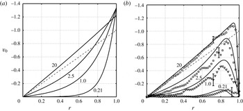
, obtained using equation (5.10), is shown in figure 7(a), at values of
 $S$
corresponding to experiments A, B, C and E.
(a) Azimuthal velocity component,
 $v_{0}$
, obtained using equation (5.10) at the mid-height
 $z=0.5h$
, and plotted against
 $r$
for a range of values of
 $S$
(labelled). Note, as
 $v_{0}$
is relative to the new rotation rate, a fully spun-up state would correspond to
 $v_{0}=0$
. The dashed line shows the initial solid-body rotation. (b) A comparison of the composite solution in equation (5.16) with measurements of
 $v_{0}$
obtained from the experiments. Here the comparison is made at the height
 $z=0.4h$
, with the experimental data taken from the azimuth
 $\unicode[STIX]{x1D703}=3\unicode[STIX]{x03C0}/2$
(i.e. the east coordinate). Again, the corresponding values of
 $S$
for each case are shown on the figure and the dashed line shows the initial solid-body rotation. Note that the experimental data for
 $S=20$
are essentially axisymmetric, whereas the data for
 $S=0.21$
, 1.0 and 2.5 are not, but instead exhibit a degree of (primarily) north–south asymmetry. In (b), the error bars show an estimate of the uncertainty in each set of data, obtained by calculating the peak root-mean-square deviation from 30 velocity profiles about each profile shown (corresponding to a period of 3 s).

Finally, notice that
 $$\begin{eqnarray}\displaystyle \unicode[STIX]{x1D70E}=\mathop{\sum }_{n=1}^{\infty }\frac{\tanh (\unicode[STIX]{x1D707}_{n0}h/2)}{\unicode[STIX]{x1D6FC}_{n0}^{3}}<\frac{S^{1/2}}{4}h\mathop{\sum }_{n=1}^{\infty }\frac{1}{\unicode[STIX]{x1D6FC}_{n0}^{2}}, & & \displaystyle\end{eqnarray}$$
and the sum
 $\sum 1/\unicode[STIX]{x1D6FC}_{n0}^{2}=1/4$
(Sneddon Reference Sneddon1960), so we have
 $$\begin{eqnarray}\displaystyle \frac{16\unicode[STIX]{x1D70E}}{hS^{1/2}}<1, & & \displaystyle\end{eqnarray}$$
so the denominator in the
 $v_{0}$
expression is always positive and never zero.
5.2 Sidewall boundary layers and the composite motion
In Munro & Foster (Reference Munro and Foster2014) – but in more detail in Foster & Munro (Reference Foster and Munro2012) and Munro et al. (Reference Munro, Hewitt and Foster2015) – we have shown that even at small Rossby numbers, the sidewall boundary layers are fully nonlinear Prandtl boundary layers, and as such are subject to spatio-temporal eruption at finite times – the mechanism for the formation of vertical vortices in these flows. Indeed, Munro et al. (Reference Munro, Hewitt and Foster2015) provided a strong affirmation of that mechanism in experimental results, boundary-layer computations and Navier–Stokes calculations. However, for times not too long, the sidewall boundary layers begin as Rayleigh layers, well known to have physical thickness
 $(\unicode[STIX]{x1D708}t^{\ast })^{1/2}$
, or
 $(Et)^{1/2}$
in our dimensionless notation. On the time scales investigated in the analysis in this paper, where
 $t\sim E^{-1/2}$
, such layers obviously scale like
 $E^{1/4}$
. Neglect of the nonlinear terms on this short time scale requires that
 $t\ll \unicode[STIX]{x1D716}^{-1}$
, guaranteed under the proviso that
 $\unicode[STIX]{x1D716}\ll E^{1/2}$
, as we have already noted.
Hence, the Rayleigh-layer equation for the azimuthal velocity component near the sidewall is
 $$\begin{eqnarray}\displaystyle \bar{v}_{\bar{t}}=\bar{v}_{\bar{r}\bar{r}}, & & \displaystyle\end{eqnarray}$$
where
 $r=1-E^{1/4}\bar{r}$
and
 $t=E^{-1/2}\bar{t}$
. The solution is well known, namely,
 $$\begin{eqnarray}\displaystyle \bar{v}=v_{0}(1,\unicode[STIX]{x1D703},z,\unicode[STIX]{x1D702}\unicode[STIX]{x1D70F})\text{erf}\left(\frac{\bar{r}}{2\sqrt{\bar{t}}}\right). & & \displaystyle\end{eqnarray}$$
Note that
 $\unicode[STIX]{x1D703}$
and
 $z$
variations in the flow at the edge of the layer are parametric in the solution.
Then, for
 $\unicode[STIX]{x1D702}\unicode[STIX]{x1D70F}\rightarrow \infty$
, the ‘steady state’ discussed above is achieved for
 $v_{0}$
, but the Rayleigh layer is still thickening in time. In this narrow segment of time, we may form a quasi-steady velocity profile for the horizontal motion outside the upper and lower bounding surfaces as an additive composite, that is
 $$\begin{eqnarray}\displaystyle v=v_{0}(r,\unicode[STIX]{x1D703},z,\infty )\text{erfc}\left(\frac{1-r}{2\sqrt{Et}}\right). & & \displaystyle\end{eqnarray}$$
We plot in figure 7(b) this composite azimuthal velocity profile compared with measured velocity data from four of the experiments listed in table 1. Recall, the ‘steady state’ solution corresponds not to when the fluid is fully spun up, but to when the slope-induced flow features have effectively been damped by the stratification and friction. Hence, we have attempted to make the comparisons at times that satisfy this condition. For
 $S=20$
, the comparison time was chosen based on the large-
 $S$
analysis presented in § 6 below. There we show that the Rossby modes are damped as
 $\exp [\unicode[STIX]{x1D706}(\unicode[STIX]{x1D6FC}\unicode[STIX]{x1D6FA}S^{1/2}t^{\ast })]$
, and so the comparison time was chosen to be
 $t^{\ast }=1/|\unicode[STIX]{x1D706}|\unicode[STIX]{x1D6FC}\unicode[STIX]{x1D6FA}S^{1/2}$
, where
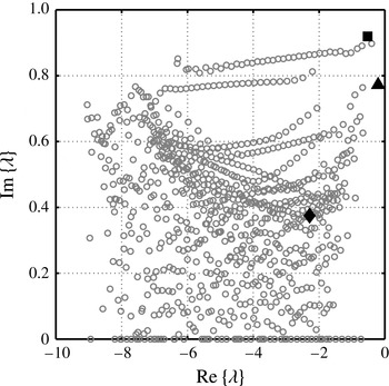
 $\unicode[STIX]{x1D706}=-0.2$
is the computed eigenvalue corresponding to the slowest damped mode (see § 6.3.2 below). The corresponding time for
 $S=20$
(Exp E) was
 $\unicode[STIX]{x1D6FC}\unicode[STIX]{x1D6FA}t^{\ast }=3.2$
. For
 $S=0.21$
, 1.0 and 2.5, the comparison times were chosen based on visual inspection of the streamline data, when the formation of Rossby waves had ceased: these were
 $\unicode[STIX]{x1D6FC}\unicode[STIX]{x1D6FA}t^{\ast }=34$
, 14 and 9.1 for
 $S=0.21$
(Exp A),
 $S=1.0$
(Exp B) and
 $S=2.5$
(Exp C) respectively. We note that the data for
 $S=10$
(Exp D) were little different from the
 $S=20$
data, and so have not be included in figure 7(b), to avoid over saturation of data points. Unsurprisingly, the data for
 $S=20$
, which are essentially axisymmetric throughout, are in very good agreement with the theoretical prediction. At the smaller values of
 $S$
shown the agreement is generally good, although is clearly affected by a degree of asymmetry that is evident in the experimental data at the times at which the comparison is made.
5.3 The final, viscous decay
Friction at top and bottom surfaces causes the decay of the Rossby waves, the process ending with the steady state given in the above section. In a linearly stratified fluid the final ‘spun-up’ state is achieved on the diffusive time scale
 $E^{-1}\unicode[STIX]{x1D6FA}^{-1}$
, unlike the case for a homogeneous fluid where the spun-up state is reached more rapidly on the much shorter
 $E^{-1/2}\unicode[STIX]{x1D6FA}^{-1}$
time scale (Walin Reference Walin1969). The final stage of the decay has been explored by Duck & Foster (Reference Duck and Foster2001), on a time scale
 $\tilde{t}\equiv Et$
. That discussion is for an axisymmetric situation only, but we have seen above that this flow is in fact axisymmetric beyond the spin-up times. We do not repeat the analysis here, but the solution may be written as
 $$\begin{eqnarray}\displaystyle v=\mathop{\sum }_{n=1}^{\infty }H_{n}(z,\tilde{t})J_{1}(\unicode[STIX]{x1D6FC}_{1n}r), & & \displaystyle\end{eqnarray}$$
and the coefficient function is itself a Fourier sine series in
 $z$
,
 $$\begin{eqnarray}\displaystyle H_{n}=\mathop{\sum }_{m=1}^{\infty }h_{nm}(\tilde{t})\sin (m\unicode[STIX]{x03C0}z/h), & & \displaystyle\end{eqnarray}$$
where the sine series coefficient is
 $$\begin{eqnarray}\displaystyle h_{nm}=h_{nm}(0)\text{e}^{-\unicode[STIX]{x1D714}_{nm}\tilde{t}}. & & \displaystyle\end{eqnarray}$$
Substitution into the appropriate equations in this time range, as given in Duck & Foster (Reference Duck and Foster2001), leads to a formula for the time decay coefficients
 $$\begin{eqnarray}\displaystyle \unicode[STIX]{x1D714}_{nm}=\frac{S}{4}\unicode[STIX]{x1D6FC}_{1n}^{2}\frac{m^{2}\unicode[STIX]{x03C0}^{2}+\unicode[STIX]{x1D6FC}_{1n}^{2}h^{2}}{m^{2}\unicode[STIX]{x03C0}^{2}+(S/4)\unicode[STIX]{x1D6FC}_{1n}^{2}h^{2}}. & & \displaystyle\end{eqnarray}$$
The value of
 $h_{nm}(0)$
is found from the initial condition for this motion – the steady state from (5.8) – by means of the orthogonality of the sine series and the Fourier–Bessel series. Doing that results in
 $$\begin{eqnarray}\displaystyle & \displaystyle h_{nm}(0)=\frac{2K_{3}}{S}\left[\mathop{\sum }_{k=1}^{\infty }\frac{c_{k}\unicode[STIX]{x1D6E4}_{kn}m\unicode[STIX]{x03C0}}{\unicode[STIX]{x1D6FC}_{0k}}\frac{1-(-1)^{m}}{m^{2}\unicode[STIX]{x03C0}^{2}+\unicode[STIX]{x1D707}_{0k}^{2}h^{2}}\right]-\mathop{\sum }_{k=1}^{\infty }\frac{1-(-1)^{m}}{m\unicode[STIX]{x03C0}\unicode[STIX]{x1D6FC}_{0k}}\frac{c_{k}\unicode[STIX]{x1D707}_{0k}^{2}h^{2}\unicode[STIX]{x1D6E4}_{kn}}{m^{2}\unicode[STIX]{x03C0}^{2}+\unicode[STIX]{x1D707}_{0k}^{2}h^{2}}, & \displaystyle \nonumber\\ \displaystyle & & \displaystyle\end{eqnarray}$$
 $$\begin{eqnarray}\displaystyle & \displaystyle \unicode[STIX]{x1D6E4}_{kn}=\frac{2J_{1}(\unicode[STIX]{x1D6FC}_{0k})}{(\unicode[STIX]{x1D6FC}_{0k}^{2}-\unicode[STIX]{x1D6FC}_{1n}^{2})J_{0}(\unicode[STIX]{x1D6FC}_{1n})}. & \displaystyle\end{eqnarray}$$
 $\unicode[STIX]{x1D714}_{nm}$
.
This viscous decay was examined using experiment E (
 $S=20$
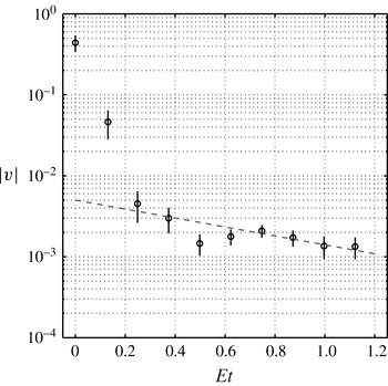
), which was run over a period of several hours. In § 2 we showed that, under these conditions, the flow within the bulk interior remained largely axisymmetric throughout (see figure 6). Figure 8 shows measurements taken from experiment E of the azimuthal speed,
 $|v|$
, at the interior point
 $r=0.5$
,
 $\unicode[STIX]{x1D703}=3\unicode[STIX]{x03C0}/2$
,
 $z=0.4h$
. The data are shown (circles) on semi-log-scale and are consistent with the decay rate computed from
 $\unicode[STIX]{x1D714}_{11}$
, which is shown as the broken line.
The circles show measurements from Experiment E (
 $S=20$
) of the azimuthal speed
 $|v|$
at the point
 $r=0.5$
,
 $\unicode[STIX]{x1D703}=3\unicode[STIX]{x03C0}/2$
,
 $z=0.4h$
. The broken line shows decay proportional to
 $\exp (-\unicode[STIX]{x1D714}_{11}Et)$
, with
 $\unicode[STIX]{x1D714}_{11}=1.271$
. Note that,
 $Et=1$
corresponds to the viscous time scale
 $E^{-1}\unicode[STIX]{x1D6FA}^{-1}$
, which in this case is
 ${\approx}8~\text{h}$
. The error bars show an estimate of the uncertainty in each measurement, and are based on the time-averaged root-mean-square deviation in the data (over durations of 3 s at the early times and up to 1 min at the much later times).

6 Large-
$S$
case

Taking
 $S$
to be large, and based on insight from the exact solution, we note that the general solution to equation (5.2), that satisfies the Dirichlet condition on
 $r=1$
, is
 $$\begin{eqnarray}\displaystyle p_{0}=C(\unicode[STIX]{x1D70F}^{\prime })(r^{2}-1)+\frac{S}{2}[1-C(\unicode[STIX]{x1D70F}^{\prime })]z(z-h)+X(\unicode[STIX]{x1D70F}^{\prime })z, & & \displaystyle\end{eqnarray}$$
where times now scale with the buoyancy frequency, not the rotation rate, so
 $$\begin{eqnarray}\displaystyle \unicode[STIX]{x1D70F}^{\prime }=S^{1/2}\unicode[STIX]{x1D70F}. & & \displaystyle\end{eqnarray}$$
Note that there are several orders in this equation – order one through order
 $S$
. We note from the exact solution for all
 $S$
that the ‘steady-state’ solution is symmetric about the mid-plane; a non-zero value of
 $X$
clearly indicates a lack of top-to-bottom symmetry of the core flow.
6.1 Overview of the motion
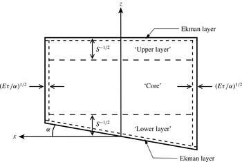
The mathematical details of this fully three-dimensional flow are algebraically complicated, as we shall see, so it is important to outline the overall flow structure and interactions between regions before proceeding. Figure 9 shows a basic sketch of the flow structure. From (6.1), the motion in the interior ‘core’ of the cylinder is axisymmetric, and the azimuthal velocity component is
 $z$
-independent. All of the vertical structure and non-axisymmetry is confined to thin layers of height
 $S^{-1/2}$
below the top and above the bottom boundary, i.e. the ‘upper’ and ‘lower’ layers shown in figure 9. This large-
 $S$
structure of these waves is well known, probably first noted by Walin (Reference Walin1969), but also discussed by Rhines (Reference Rhines1970), who pointed out that the large stratification – that is, large
 $S$
– inhibits vertical motion in the core; only near the lower wall does the geometric forcing stretch the vortex lines to generate waves; further, the decay to the interior is exponential.
Requiring that
 $S\ll 1/\unicode[STIX]{x1D6FC}^{2}$
assures that the sloping surface is wholly contained within this
 $S^{-1/2}$
lower layer. The temporal evolution of
 $C$
and
 $X$
in (6.1) is determined by matching to the upper and lower layers. Because of the linearity of the problem, we can most easily decompose
 $C$
and
 $X$
into various components.
Because of the three zones (core, upper layer and lower layer), and the various motions that occur within those zones, we need to supply some decoding help for the reader. Once the general formulation is given below, we consider first the steady-state values for
 $C$
and
 $X$
, corresponding to the limit
 $\unicode[STIX]{x1D70F}^{\prime }\rightarrow \infty$
. We denote those values simply by
 $C$
and
 $X$
, with no other notation. The amplitudes of the unsteady components, with a time dependence
 $\exp (\unicode[STIX]{x1D706}\unicode[STIX]{x1D70F}^{\prime })$
, are denoted by
 $c$
and
 $\unicode[STIX]{x1D712}$
respectively. However, there are two differing sorts of motion in the upper and lower layers: there are modes that decay because of top and bottom friction, and the amplitudes
 $c$
and
 $\unicode[STIX]{x1D712}$
that correspond to those unsteady motions are denoted by
 $c_{f}$
and
 $\unicode[STIX]{x1D712}_{f}$
. In the discussion of the Rossby-wave modes, no added notation is utilized, since there is no ambiguity there. Within the upper and lower layers, there are other quantities denoted by, for example,
 $k_{\ell }$
and
 $k_{u}$
, for upper- and lower-layer properties. Such quantities associated with frictional modes are similarly denoted by
 $k_{\ell f}$
and
 $k_{uf}$
. In the end, then,
 $C$
is a superposition of the steady-state value, a sum over all frictional modes, and a sum over all Rossby-wave modes.
Finally, a word about the Rossby waves themselves. One can relatively easily work out the spectrum of the waves over a sloping wall in a circular container. However, as is evident in the analysis of § 5, and will also emerge below, the spectrum for waves involved in spin-up is more complicated than a näive approach suggests. First, the eruption of Ekman fluid in the lower corners of the tank alters the spectrum; the presence of the
 $\unicode[STIX]{x1D70E}$
term in (5.8) is evidence of that in the
 $S=O(1)$
case. Secondly, the lower-layer dynamics is coupled to the interior core and upper-layer motion in a fashion that also alters the Rossby-wave spectrum.
Below, we begin with the upper-layer motion, then examine the lower-layer dynamics which includes the Rossby waves, and, throughout, match the regions together in a way the ultimately gives the evolution of
 $C$
and
 $X$
in time.
Schematic of the flow structure for large
 $S$
.

6.2 Upper layer
Near the upper surface, we write
 $z=h+S^{-1/2}\unicode[STIX]{x1D701}$
, in which case (5.2) becomes
 $$\begin{eqnarray}\displaystyle \unicode[STIX]{x1D6FB}_{1}^{2}P+4P_{\unicode[STIX]{x1D701}\unicode[STIX]{x1D701}}=-4, & & \displaystyle\end{eqnarray}$$
where
 $P$
denotes the solution for
 $p_{0}$
in this layer. The boundary condition (3.7b
) becomes,
 $$\begin{eqnarray}\displaystyle P_{\unicode[STIX]{x1D701}\unicode[STIX]{x1D70F}^{\prime }}=-\unicode[STIX]{x1D702}-\unicode[STIX]{x1D702}P_{\unicode[STIX]{x1D701}\unicode[STIX]{x1D701}}+\mathscr{E}_{h}. & & \displaystyle\end{eqnarray}$$
The general form of the solution in this axisymmetric layer, based on the matching requirements to (6.1), is
 $$\begin{eqnarray}\displaystyle P=\mathop{\sum }_{m=1}^{\infty }A_{m}(\unicode[STIX]{x1D701},\unicode[STIX]{x1D70F}^{\prime })J_{0}(\unicode[STIX]{x1D6FC}_{m0}r)-C(r^{2}-1)+\frac{1}{2}(C-1)\unicode[STIX]{x1D701}^{2}+K_{u}\unicode[STIX]{x1D701}. & & \displaystyle\end{eqnarray}$$
Matching this solution to the solution in the core, (6.1), leads to the connection
 $$\begin{eqnarray}\displaystyle K_{u}=-\frac{hS^{1/2}}{2}(1-C)+\frac{X}{S^{1/2}}. & & \displaystyle\end{eqnarray}$$
Using the facts,
 $$\begin{eqnarray}\displaystyle \int _{0}^{1}rJ_{0}(\unicode[STIX]{x1D6FC}_{m0}r)\,\text{d}r=\frac{J_{1}(\unicode[STIX]{x1D6FC}_{m0})}{\unicode[STIX]{x1D6FC}_{m0}},\quad \int _{0}^{1}r[J_{0}(\unicode[STIX]{x1D6FC}_{m0}r)]^{2}\,\text{d}r=\frac{J_{1}^{2}(\unicode[STIX]{x1D6FC}_{m0})}{2}, & & \displaystyle\end{eqnarray}$$
and requiring that the averaged velocity be zero over
 $z=h$
leads to
 $$\begin{eqnarray}\displaystyle 2\unicode[STIX]{x03C0}\mathop{\sum }_{m=1}^{\infty }A_{m,\unicode[STIX]{x1D701}\unicode[STIX]{x1D70F}}\int _{0}^{1}rJ_{0}(\unicode[STIX]{x1D6FC}_{m0}r)\,\text{d}r+\unicode[STIX]{x03C0}K_{u,\unicode[STIX]{x1D70F}^{\prime }}=0,\quad \unicode[STIX]{x1D701}=0, & & \displaystyle\end{eqnarray}$$
or
 $$\begin{eqnarray}\displaystyle \mathop{\sum }_{m=1}^{\infty }A_{m,\unicode[STIX]{x1D701}\unicode[STIX]{x1D70F}^{\prime }}\frac{J_{1}(\unicode[STIX]{x1D6FC}_{m0})}{\unicode[STIX]{x1D6FC}_{m0}}+\frac{1}{2}K_{u,\unicode[STIX]{x1D70F}^{\prime }}=0,\quad \unicode[STIX]{x1D701}=0, & & \displaystyle\end{eqnarray}$$
and, on integrating and using the homogeneous initial conditions as required,
 $$\begin{eqnarray}\displaystyle K_{u}=-2\mathop{\sum }_{m=1}^{\infty }A_{m,\unicode[STIX]{x1D701}}\frac{J_{1}(\unicode[STIX]{x1D6FC}_{m0})}{\unicode[STIX]{x1D6FC}_{m0}}. & & \displaystyle\end{eqnarray}$$
Using the orthogonality of the members of the Bessel function series, the wall boundary condition (6.4) becomes
 $$\begin{eqnarray}\displaystyle (A_{m,\unicode[STIX]{x1D701}\unicode[STIX]{x1D70F}^{\prime }}+\unicode[STIX]{x1D702}A_{m,\unicode[STIX]{x1D701}\unicode[STIX]{x1D701}})\frac{1}{2}J_{1}^{2}(\unicode[STIX]{x1D6FC}_{m0})=-(\unicode[STIX]{x1D702}C+K_{u,\unicode[STIX]{x1D70F}^{\prime }})\frac{J_{1}(\unicode[STIX]{x1D6FC}_{m0})}{\unicode[STIX]{x1D6FC}_{m0}}\quad \text{on}~\unicode[STIX]{x1D701}=0. & & \displaystyle\end{eqnarray}$$
From (6.3), the equation satisfied by
 $A_{m}$
is
 $$\begin{eqnarray}\displaystyle A_{m,\unicode[STIX]{x1D701}\unicode[STIX]{x1D701}}-\frac{\unicode[STIX]{x1D6FC}_{m0}^{2}}{4}A_{m}=0, & & \displaystyle\end{eqnarray}$$
so the matchable solution is
 $$\begin{eqnarray}\displaystyle A_{m}=a_{m}\text{e}^{\unicode[STIX]{x1D6FC}_{m0}\unicode[STIX]{x1D701}/2}. & & \displaystyle\end{eqnarray}$$
Substituting into (6.11) leads to
 $$\begin{eqnarray}\displaystyle a_{m,\unicode[STIX]{x1D70F}^{\prime }}+\frac{1}{2}\unicode[STIX]{x1D6FC}_{m0}\unicode[STIX]{x1D702}a_{m}=-(\unicode[STIX]{x1D702}C+K_{u,\unicode[STIX]{x1D70F}^{\prime }})\frac{4}{J_{1}(\unicode[STIX]{x1D6FC}_{m0})\unicode[STIX]{x1D6FC}_{m0}^{2}}. & & \displaystyle\end{eqnarray}$$
Putting in the evaluation of
 $K_{u}$
from (6.10), we have
 $$\begin{eqnarray}\displaystyle a_{m,\unicode[STIX]{x1D70F}^{\prime }}+\frac{1}{2}\unicode[STIX]{x1D6FC}_{m0}\unicode[STIX]{x1D702}a_{m}=\frac{4}{J_{1}(\unicode[STIX]{x1D6FC}_{m0})\unicode[STIX]{x1D6FC}_{m0}^{2}}\left[-\unicode[STIX]{x1D702}C+\mathop{\sum }_{r=1}^{\infty }a_{r,\unicode[STIX]{x1D70F}^{\prime }}J_{1}(\unicode[STIX]{x1D6FC}_{r0})\right]. & & \displaystyle\end{eqnarray}$$
6.2.1 Steady state
The particular solution to (6.15) corresponds to the long-time behaviour (
 $\unicode[STIX]{x1D702}\unicode[STIX]{x1D70F}^{\prime }\rightarrow \infty$
), after the transient, and is clearly given simply by
 $$\begin{eqnarray}\displaystyle \tilde{a}_{m}=-\frac{8C}{\unicode[STIX]{x1D6FC}_{m0}^{3}J_{1}(\unicode[STIX]{x1D6FC}_{m0})}, & & \displaystyle\end{eqnarray}$$
letting
 $\tilde{a}_{m}$
denote the particular solution for
 $a_{m}$
.
Multiplying by
 $J_{1}(\unicode[STIX]{x1D6FC}_{m0})$
and summing over
 $m$
gives the steady-state relation between
 $K_{u}$
and
 $C$
as
 $$\begin{eqnarray}\displaystyle K_{u}=8C\mathop{\sum }_{m=1}^{\infty }\frac{1}{\unicode[STIX]{x1D6FC}_{m0}^{3}}. & & \displaystyle\end{eqnarray}$$
Combining with (6.6), we find a relationship between
 $C$
and
 $X$
, namely
 $$\begin{eqnarray}\displaystyle -\frac{S^{1/2}}{2}h(1-C)+\frac{X}{S^{1/2}}=8C\mathop{\sum }_{m=1}^{\infty }\frac{1}{\unicode[STIX]{x1D6FC}_{m0}^{3}}. & & \displaystyle\end{eqnarray}$$
Thus, we have a steady-state relationship between
 $C$
and
 $X$
,
 $$\begin{eqnarray}\displaystyle C=\left(1-\frac{16}{S^{1/2}h}\mathop{\sum }_{m=1}^{\infty }\frac{1}{\unicode[STIX]{x1D6FC}_{m0}^{3}}\right)^{-1}\left(1-\frac{2X}{Sh}\right). & & \displaystyle\end{eqnarray}$$
The completion of the steady result is in § 6.3.1, since it depends on the effects of the lower layer.
Combining gives the long-time behaviour of the pressure perturbation as
 $$\begin{eqnarray}\displaystyle P=-C\left\{8\mathop{\sum }_{m=1}^{\infty }\frac{1}{\unicode[STIX]{x1D6FC}_{m0}^{3}}\left[\text{e}^{\unicode[STIX]{x1D6FC}_{m0}\unicode[STIX]{x1D701}/2}\frac{J_{0}(\unicode[STIX]{x1D6FC}_{m0}r)}{J_{1}(\unicode[STIX]{x1D6FC}_{m0})}-\unicode[STIX]{x1D701}\right]-\frac{hS^{1/2}}{2}\unicode[STIX]{x1D701}+r^{2}-1\right\}+\frac{1}{2}(C-1)\unicode[STIX]{x1D701}^{2}. & & \displaystyle \nonumber\\ \displaystyle & & \displaystyle\end{eqnarray}$$
Evaluating the azimuthal component in the layer,
 $$\begin{eqnarray}\displaystyle v=\frac{1}{2}\frac{\unicode[STIX]{x2202}P}{\unicode[STIX]{x2202}r}=-C\left[r-4\mathop{\sum }_{m=1}^{\infty }\frac{J_{1}(\unicode[STIX]{x1D6FC}_{m0}r)}{\unicode[STIX]{x1D6FC}_{m0}^{2}J_{1}(\unicode[STIX]{x1D6FC}_{m0})}\,\text{e}^{\unicode[STIX]{x1D6FC}_{m0}\unicode[STIX]{x1D701}/2}\right]. & & \displaystyle\end{eqnarray}$$
From the properties of Bessel functions,
 $$\begin{eqnarray}\displaystyle r=\mathop{\sum }_{m=1}^{\infty }\frac{4}{\unicode[STIX]{x1D6FC}_{m0}^{2}}\,\frac{J_{1}(\unicode[STIX]{x1D6FC}_{m0}r)}{J_{1}(\unicode[STIX]{x1D6FC}_{m0})}. & & \displaystyle\end{eqnarray}$$
Thus, we see that
 $$\begin{eqnarray}\displaystyle v=0\quad \text{on}~\unicode[STIX]{x1D701}=0\;(\text{or}~z=h), & & \displaystyle\end{eqnarray}$$
so that the fluid is totally spun-up at the upper wall, but the velocity grows rapidly away from
 $z=h$
, so that in the interior, the velocity is
 $Cr$
.
6.2.2 Unsteadiness
The time dependence of the motion is determined by putting
 $a_{m}=\hat{a}_{m}\exp (\unicode[STIX]{x1D706}\unicode[STIX]{x1D70F}^{\prime })$
into the homogeneous version of (6.14), leading to the eigenvalue problem
 $$\begin{eqnarray}\displaystyle \left(\unicode[STIX]{x1D706}+\frac{1}{2}\unicode[STIX]{x1D702}\unicode[STIX]{x1D6FC}_{m0}\right)\hat{a}_{m}=\frac{4}{\unicode[STIX]{x1D6FC}_{m0}^{2}J_{1}(\unicode[STIX]{x1D6FC}_{m0})}\left(-\unicode[STIX]{x1D702}c-\unicode[STIX]{x1D706}k_{u}\right), & & \displaystyle\end{eqnarray}$$
where we have also written
 $K_{u}=k_{u}\exp (\unicode[STIX]{x1D706}\unicode[STIX]{x1D70F}^{\prime })$
and
 $C=c\exp (\unicode[STIX]{x1D706}\unicode[STIX]{x1D70F}^{\prime })$
. Solving for
 $\hat{a}_{m}J_{1}(\unicode[STIX]{x1D6FC}_{m0})$
, and then summing,
 $$\begin{eqnarray}\displaystyle k_{u}=4\mathop{\sum }_{m=1}^{\infty }\frac{1}{\unicode[STIX]{x1D6FC}_{m0}^{2}\left(\unicode[STIX]{x1D706}+\frac{1}{2}\unicode[STIX]{x1D702}\unicode[STIX]{x1D6FC}_{m0}\right)}(\unicode[STIX]{x1D702}c+\unicode[STIX]{x1D706}k_{u}). & & \displaystyle\end{eqnarray}$$
Putting
 $X=\unicode[STIX]{x1D712}\exp (\unicode[STIX]{x1D706}\unicode[STIX]{x1D70F}^{\prime })$
, and using (6.6) to relate
 $c$
and
 $k_{u}$
to
 $\unicode[STIX]{x1D712}$
leads eventually to
 $$\begin{eqnarray}\displaystyle k_{u}\left[\left(\unicode[STIX]{x1D706}+\frac{2\unicode[STIX]{x1D702}}{hS^{1/2}}\right)\mathop{\sum }_{m=1}^{\infty }\frac{1}{\unicode[STIX]{x1D6FC}_{m0}^{2}\left(\unicode[STIX]{x1D706}+\frac{1}{2}\unicode[STIX]{x1D702}\unicode[STIX]{x1D6FC}_{m0}\right)}-\frac{1}{4}\right]=\unicode[STIX]{x1D702}\frac{2\unicode[STIX]{x1D712}}{hS}\mathop{\sum }_{m=1}^{\infty }\frac{1}{\unicode[STIX]{x1D6FC}_{m0}^{2}\left(\unicode[STIX]{x1D706}+\frac{1}{2}\unicode[STIX]{x1D702}\unicode[STIX]{x1D6FC}_{m0}\right)}. & & \displaystyle \nonumber\\ \displaystyle & & \displaystyle\end{eqnarray}$$
Two possible scalings arise of these equations, delineated below.
-
(i)
$\unicode[STIX]{x1D706}=O(1)$
: Rossby waves
We know that there are Rossby waves in the container, so
$\unicode[STIX]{x1D706}=O(1)$
as
$\unicode[STIX]{x1D702}\rightarrow 0$
for the waves. The
$1/4$
in the square bracket in (6.26) may be replaced by
$\sum _{m=1}^{\infty }1/\unicode[STIX]{x1D6FC}_{m0}^{2}$
, as previously quoted from Sneddon (Reference Sneddon1960), and the two terms in the square bracket in equation become, without approximation, (6.27)As
$$\begin{eqnarray}\displaystyle \frac{2\unicode[STIX]{x1D702}}{hS^{1/2}}\mathop{\sum }_{m=1}^{\infty }\frac{1}{\unicode[STIX]{x1D6FC}_{m0}^{2}\left(\unicode[STIX]{x1D706}+\frac{1}{2}\unicode[STIX]{x1D702}\unicode[STIX]{x1D6FC}_{m0}\right)}-\frac{\unicode[STIX]{x1D702}}{2}\mathop{\sum }_{m=1}^{\infty }\frac{1}{\unicode[STIX]{x1D6FC}_{m0}\left(\unicode[STIX]{x1D706}+\frac{1}{2}\unicode[STIX]{x1D702}\unicode[STIX]{x1D6FC}_{m0}\right)}. & & \displaystyle\end{eqnarray}$$
$\unicode[STIX]{x1D702}\rightarrow 0$
, the second of these series is divergent, and in fact behaves like
$\log \unicode[STIX]{x1D702}$
– see Munro & Foster (Reference Munro and Foster2014). Note that, therefore, (6.26) determines
$k_{u}$
to be of order
$\unicode[STIX]{x1D712}/\log \unicode[STIX]{x1D702}$
, so the
$k_{u}$
term is negligible in (6.6), leading to (6.28)Note that this relationship between
$$\begin{eqnarray}\displaystyle \frac{hS^{1/2}}{2}c+\frac{\unicode[STIX]{x1D712}}{S^{1/2}}=0. & & \displaystyle\end{eqnarray}$$
$c$
and
$\unicode[STIX]{x1D712}$
is valid only on the Rossby-wave scale.
-
(ii)
$\unicode[STIX]{x1D706}=O(\unicode[STIX]{x1D702})$
: frictional decay
In this case, we write
$\unicode[STIX]{x1D706}=\unicode[STIX]{x1D702}\unicode[STIX]{x1D6EC}$
, in which case, (6.26) becomes (6.29)Recall that we have appended an
$$\begin{eqnarray}\displaystyle k_{uf}\left[\left(\unicode[STIX]{x1D6EC}+\frac{2}{hS^{1/2}}\right)\mathop{\sum }_{m=1}^{\infty }\frac{1}{\unicode[STIX]{x1D6FC}_{m0}^{2}\left(\unicode[STIX]{x1D6EC}+\frac{1}{2}\unicode[STIX]{x1D6FC}_{m0}\right)}-\frac{1}{4}\right]=\frac{2\unicode[STIX]{x1D712}_{f}}{hS}\mathop{\sum }_{m=1}^{\infty }\frac{1}{\unicode[STIX]{x1D6FC}_{m0}^{2}\left(\unicode[STIX]{x1D6EC}+\frac{1}{2}\unicode[STIX]{x1D702}\unicode[STIX]{x1D6FC}_{m0}\right)}. & & \displaystyle \nonumber\\ \displaystyle & & \displaystyle\end{eqnarray}$$
$f$
-subscript to distinguish those elements of
$c$
,
$\unicode[STIX]{x1D712}$
and
$k_{u}$
that are associated with frictional decay only, with unsubscripted values of
$c,\unicode[STIX]{x1D712}$
and
$k_{u}$
corresponding to Rossby waves. In addition, (6.25) is (6.30)
$$\begin{eqnarray}\displaystyle k_{uf}=4\mathop{\sum }_{m=1}^{\infty }\frac{1}{\unicode[STIX]{x1D6FC}_{m0}^{2}\left(\unicode[STIX]{x1D6EC}+\frac{1}{2}\unicode[STIX]{x1D6FC}_{m0}\right)}(c_{f}+\unicode[STIX]{x1D6EC}k_{uf}). & & \displaystyle\end{eqnarray}$$


As we shall determine in § 6.3.3, in the lower
 $S^{-1/2}$
layer, on this time scale, the relationship between
 $c$
and
 $\unicode[STIX]{x1D712}$
is given as (6.60), namely
 $$\begin{eqnarray}\displaystyle \left(8\mathop{\sum }_{m=1}^{\infty }\frac{1}{\unicode[STIX]{x1D6FC}_{m0}^{3}}-\frac{hS^{1/2}}{2}\right)c=-\frac{\unicode[STIX]{x1D712}}{S^{1/2}}. & & \displaystyle\end{eqnarray}$$
Combining with (6.30) and (6.29), and after some algebra, gives the eigenvalue problem
 $$\begin{eqnarray}\displaystyle \left[\unicode[STIX]{x1D6EC}-\left(8\mathop{\sum }_{m=1}^{\infty }1/\unicode[STIX]{x1D6FC}_{m0}^{3}-hS^{1/2}\right)^{-1}\right]\mathop{\sum }_{m=1}^{\infty }\frac{1}{\unicode[STIX]{x1D6FC}_{m0}^{2}\left(\unicode[STIX]{x1D6EC}+\frac{1}{2}\unicode[STIX]{x1D6FC}_{m0}\right)}-\frac{1}{4}=0. & & \displaystyle\end{eqnarray}$$
Neglecting for now the
 $S^{-1/2}$
corrections, this becomes
 $$\begin{eqnarray}\displaystyle \mathop{\sum }_{m=1}^{\infty }\frac{\unicode[STIX]{x1D6EC}}{\unicode[STIX]{x1D6FC}_{m0}^{2}\left(\unicode[STIX]{x1D6EC}+\frac{1}{2}\unicode[STIX]{x1D6FC}_{m0}\right)}=\frac{1}{4}. & & \displaystyle\end{eqnarray}$$
Assume that
 $\unicode[STIX]{x1D6EC}$
has non-zero imaginary part. Multiply (6.33) by the conjugate of
 $\unicode[STIX]{x1D6EC}$
. Then multiplying numerator and denominator of the term in the sum by the conjugate of
 $\unicode[STIX]{x1D6EC}+\unicode[STIX]{x1D6FC}_{m0}/2$
, and taking the imaginary part of the equation leads to the result, for non-zero imaginary part of
 $\unicode[STIX]{x1D6EC}$
,
 $$\begin{eqnarray}\displaystyle \frac{1}{4|\unicode[STIX]{x1D6EC}|^{2}}=\mathop{\sum }_{m=1}^{\infty }\frac{1}{\unicode[STIX]{x1D6FC}_{m0}^{2}|\unicode[STIX]{x1D6EC}+\frac{1}{2}\unicode[STIX]{x1D6FC}_{m0}|^{2}}. & & \displaystyle\end{eqnarray}$$
Clearly,
 $|\unicode[STIX]{x1D6EC}+(1/2)\unicode[STIX]{x1D6FC}_{m0}|^{2}\geqslant |\unicode[STIX]{x1D6EC}|^{2}$
by use of the triangle inequality. However, these two quantities can be equal only if
 $\unicode[STIX]{x1D6FC}_{m0}$
is zero, which it cannot be. Hence,
 $|\unicode[STIX]{x1D6EC}+(1/2)\unicode[STIX]{x1D6FC}_{m0}|^{2}>|\unicode[STIX]{x1D6EC}|^{2}$
, so we have
 $$\begin{eqnarray}\displaystyle \frac{1}{4}<\mathop{\sum }_{m=1}^{\infty }\frac{1}{\unicode[STIX]{x1D6FC}_{m0}^{2}}, & & \displaystyle\end{eqnarray}$$
which is a contradiction, since
 $\sum _{m=1}^{\infty }1/\unicode[STIX]{x1D6FC}_{m0}^{2}=1/4$
. Therefore,
 $\unicode[STIX]{x1D6EC}$
can have no imaginary part.
So, if
 $\unicode[STIX]{x1D6EC}$
is purely real, assume that it is positive. In that case,
 $$\begin{eqnarray}\displaystyle \mathop{\sum }_{m=1}^{\infty }\frac{1}{\unicode[STIX]{x1D6FC}_{m0}^{2}\left(\unicode[STIX]{x1D6EC}+\frac{1}{2}\unicode[STIX]{x1D6FC}_{m0}\right)}<\frac{1}{\unicode[STIX]{x1D6EC}}\mathop{\sum }_{m=1}^{\infty }\frac{1}{\unicode[STIX]{x1D6FC}_{m0}^{2}}=\frac{1}{4\unicode[STIX]{x1D6EC}}, & & \displaystyle\end{eqnarray}$$
which contradicts (6.33), so we conclude that
 $$\begin{eqnarray}\displaystyle \unicode[STIX]{x1D6EC}\;\text{is real and negative}, & & \displaystyle\end{eqnarray}$$
for all solutions of (6.33).
The eigenvalue equation (6.33) may alternatively be written in the simpler form
 $$\begin{eqnarray}\displaystyle \mathop{\sum }_{m=1}^{\infty }\frac{1}{\unicode[STIX]{x1D6FC}_{m0}\left(\frac{1}{2}\unicode[STIX]{x1D6FC}_{m0}-\unicode[STIX]{x1D708}\right)}=0, & & \displaystyle\end{eqnarray}$$
where we have written
 $\unicode[STIX]{x1D6EC}=-\unicode[STIX]{x1D708}$
, and the result from Sneddon (Reference Sneddon1960) has been used again. A geometric argument from this or (6.25) leads to the fact that the values of
 $\unicode[STIX]{x1D708}$
interlace with
 $\{\unicode[STIX]{x1D6FD}_{i}\}/2$
, that is, for the
 $j$
th eigenvalue,
 $$\begin{eqnarray}\displaystyle {\textstyle \frac{1}{2}}\unicode[STIX]{x1D6FD}_{j}<\unicode[STIX]{x1D708}_{j}<{\textstyle \frac{1}{2}}\unicode[STIX]{x1D6FD}_{j+1},\quad j=1,2,3,\ldots . & & \displaystyle\end{eqnarray}$$
For every solution to (6.38)
 $\unicode[STIX]{x1D708}_{j}$
, there corresponds a solution to (6.24), so the general solution for
 $\hat{a}_{n}$
is constituted by a linear combination of all possible solutions, that is
 $$\begin{eqnarray}\displaystyle \hat{a}_{n}=\mathop{\sum }_{j=1}^{\infty }c_{nj}\text{e}^{-\unicode[STIX]{x1D702}\unicode[STIX]{x1D708}_{j}\unicode[STIX]{x1D70F}^{\prime }}. & & \displaystyle\end{eqnarray}$$
That being the case, for every eigenvalue, there is a value for
 $\tilde{C}$
, hence
 $$\begin{eqnarray}\displaystyle c=\mathop{\sum }_{j=1}^{\infty }c_{j}\text{e}^{-\unicode[STIX]{x1D702}\unicode[STIX]{x1D708}_{j}\unicode[STIX]{x1D70F}^{\prime }}. & & \displaystyle\end{eqnarray}$$
An important conclusion is that the core flow decays by friction –
 $C$
to a constant, and
 $X$
to zero – for
 $\unicode[STIX]{x1D702}\unicode[STIX]{x1D70F}^{\prime }\rightarrow \infty$
.
6.3 Lower layer
Proceeding much as in the layer near the upper surface, we write
 $z=S^{-1/2}\unicode[STIX]{x1D701}$
. Because the lower wall is sloped at angle
 $\unicode[STIX]{x1D6FC}$
, in order to be able to ignore slope in this layer, we require that
 $$\begin{eqnarray}\displaystyle S^{-1/2}\gg \unicode[STIX]{x1D6FC}. & & \displaystyle\end{eqnarray}$$
When
 $S^{1/2}\unicode[STIX]{x1D6FC}=O(1)$
, the slope of the lower boundary must come into the boundary condition in this layer.
We write the solution in this region in a form that guarantees matching to (6.1), namely,
 $$\begin{eqnarray}\displaystyle P & = & \displaystyle C(1-r^{2})-\frac{1}{2}(1-C)\unicode[STIX]{x1D701}^{2}+K_{\ell }(\unicode[STIX]{x1D70F}^{\prime })\unicode[STIX]{x1D701}\nonumber\\ \displaystyle & & \displaystyle +\,\mathop{\sum }_{m=1}^{\infty }\mathop{\sum }_{n=0}^{\infty }a_{mn}(\unicode[STIX]{x1D70F}^{\prime })\text{e}^{-\unicode[STIX]{x1D6FC}_{mn}\unicode[STIX]{x1D701}/2}\cos (n\unicode[STIX]{x1D703})J_{n}(\unicode[STIX]{x1D6FC}_{mn}r)\nonumber\\ \displaystyle & & \displaystyle +\,\mathop{\sum }_{m=1}^{\infty }\mathop{\sum }_{n=1}^{\infty }b_{mn}(\unicode[STIX]{x1D70F}^{\prime })\text{e}^{-\unicode[STIX]{x1D6FC}_{mn}\unicode[STIX]{x1D701}/2}\sin (n\unicode[STIX]{x1D703})J_{n}(\unicode[STIX]{x1D6FC}_{mn}r).\end{eqnarray}$$
On matching,
 $$\begin{eqnarray}\displaystyle K_{\ell }=\frac{hS^{1/2}}{2}(1-C)+\frac{X}{S^{1/2}}. & & \displaystyle\end{eqnarray}$$
The boundary condition is
 $$\begin{eqnarray}\displaystyle P_{\unicode[STIX]{x1D701}\unicode[STIX]{x1D70F}^{\prime }}=\mathscr{E}_{0}+\unicode[STIX]{x1D702}P_{\unicode[STIX]{x1D701}\unicode[STIX]{x1D701}}+\frac{1}{2}\left(\sin \unicode[STIX]{x1D703}P_{r}+\frac{\cos \unicode[STIX]{x1D703}}{r}P_{\unicode[STIX]{x1D703}}\right)+\unicode[STIX]{x1D702}\quad \text{at}~\unicode[STIX]{x1D701}=0. & & \displaystyle\end{eqnarray}$$
Substitution gives
 $$\begin{eqnarray}\displaystyle & & \displaystyle K_{\ell }^{\prime }-\frac{1}{2}\mathop{\sum }_{m=1}^{\infty }\mathop{\sum }_{n=0}^{\infty }\unicode[STIX]{x1D6FC}_{mn}a_{mn}^{\prime }\cos (n\unicode[STIX]{x1D703})J_{n}(\unicode[STIX]{x1D6FC}_{mn}r)-\frac{1}{2}\mathop{\sum }_{m=1}^{\infty }\mathop{\sum }_{n=1}^{\infty }\unicode[STIX]{x1D6FC}_{mn}b_{mn}^{\prime }\sin (n\unicode[STIX]{x1D703})J_{n}(\unicode[STIX]{x1D6FC}_{mn}r)\nonumber\\ \displaystyle & & \displaystyle \quad =\frac{1}{2}\sin \unicode[STIX]{x1D703}\left[\mathop{\sum }_{m=1}^{\infty }\mathop{\sum }_{n=0}^{\infty }\unicode[STIX]{x1D6FC}_{mn}a_{mn}\cos (n\unicode[STIX]{x1D703})J_{n}^{\prime }(\unicode[STIX]{x1D6FC}_{mn}r)+\mathop{\sum }_{m=1}^{\infty }\mathop{\sum }_{n=1}^{\infty }\unicode[STIX]{x1D6FC}_{mn}b_{mn}\sin (n\unicode[STIX]{x1D703})J_{n}^{\prime }(\unicode[STIX]{x1D6FC}_{mn}r)\right]\nonumber\\ \displaystyle & & \displaystyle \qquad +\,\frac{\cos \unicode[STIX]{x1D703}}{2r}\left[-\mathop{\sum }_{m=1}^{\infty }\mathop{\sum }_{n=0}^{\infty }na_{mn}\sin (n\unicode[STIX]{x1D703})J_{n}(\unicode[STIX]{x1D6FC}_{mn}r)+\mathop{\sum }_{m=1}^{\infty }\mathop{\sum }_{n=1}^{\infty }nb_{mn}\cos (n\unicode[STIX]{x1D703})J_{n}(\unicode[STIX]{x1D6FC}_{mn}r)\right]\nonumber\\ \displaystyle & & \displaystyle \qquad +\,\frac{\unicode[STIX]{x1D702}}{4}\mathop{\sum }_{m=1}^{\infty }\mathop{\sum }_{n=0}^{\infty }\unicode[STIX]{x1D6FC}_{mn}^{2}a_{mn}\cos (n\unicode[STIX]{x1D703})J_{n}(\unicode[STIX]{x1D6FC}_{mn}r)\nonumber\\ \displaystyle & & \displaystyle \qquad +\,\frac{\unicode[STIX]{x1D702}}{4}\mathop{\sum }_{m=1}^{\infty }\mathop{\sum }_{n=1}^{\infty }\unicode[STIX]{x1D6FC}_{mn}^{2}b_{mn}\sin (n\unicode[STIX]{x1D703})J_{n}(\unicode[STIX]{x1D6FC}_{mn}r)+C\unicode[STIX]{x1D702}+rC\sin \unicode[STIX]{x1D703}+\mathscr{E}_{0}.\end{eqnarray}$$
The prime here denotes differentiation with respect to
 $\unicode[STIX]{x1D70F}^{\prime }$
. Averaging over the circle for the left-hand side terms – as above – leads to the formula for
 $K_{\ell }^{\prime }$
, which may then be integrated to give
 $$\begin{eqnarray}\displaystyle K_{\ell }=\mathop{\sum }_{m=1}^{\infty }a_{m0}(\unicode[STIX]{x1D70F}^{\prime })J_{1}(\unicode[STIX]{x1D6FC}_{m0}). & & \displaystyle\end{eqnarray}$$
Then, on using the orthogonality of the sines and cosines and also the Bessel functions gives, as in the general case in § 5 and discussed in detail in appendix A,
 $$\begin{eqnarray}\displaystyle & \displaystyle \frac{1}{2}\unicode[STIX]{x1D6FC}_{k0}a_{k0}^{\prime }+\frac{1}{4}\unicode[STIX]{x1D702}\unicode[STIX]{x1D6FC}_{k0}^{2}a_{k0}=\frac{2}{\unicode[STIX]{x1D6FC}_{k0}J_{1}(\unicode[STIX]{x1D6FC}_{k0})}(K_{\ell }^{\prime }-C\unicode[STIX]{x1D702})-\frac{1}{4}\mathop{\sum }_{m=1}^{\infty }b_{m,1}U_{mk}^{(1)}, & \displaystyle\end{eqnarray}$$
 $$\begin{eqnarray}\displaystyle & \displaystyle \frac{1}{2}\unicode[STIX]{x1D6FC}_{kn}a_{kn}^{\prime }+\frac{1}{4}\unicode[STIX]{x1D702}\unicode[STIX]{x1D6FC}_{kn}^{2}a_{kn}=-\frac{1}{4}\mathop{\sum }_{m=1}^{\infty }b_{m,n+1}U_{mk}^{(n+1)}-\frac{1}{4}\mathop{\sum }_{m=1}^{\infty }b_{m,n-1}V_{mk}^{(n-1)},\quad n=1,2,3,\ldots & \displaystyle \nonumber\\ \displaystyle & & \displaystyle\end{eqnarray}$$
 $$\begin{eqnarray}\displaystyle & \displaystyle \frac{1}{2}\unicode[STIX]{x1D6FC}_{k1}b_{k1}^{\prime }+\frac{1}{4}\unicode[STIX]{x1D702}\unicode[STIX]{x1D6FC}_{k1}^{2}b_{k1}=-\frac{1}{4}\mathop{\sum }_{m=1}^{\infty }[2a_{m0}r_{mk}^{(0)}-a_{m,2}U_{mk}^{(2)}]-\frac{2C}{\unicode[STIX]{x1D6FC}_{k1}J_{0}(\unicode[STIX]{x1D6FC}_{k1})}, & \displaystyle\end{eqnarray}$$
 $$\begin{eqnarray}\displaystyle & \displaystyle \frac{1}{2}\unicode[STIX]{x1D6FC}_{kn}b_{kn}^{\prime }+\frac{1}{4}\unicode[STIX]{x1D702}\unicode[STIX]{x1D6FC}_{kn}^{2}b_{kn}=\frac{1}{4}\mathop{\sum }_{m=1}^{\infty }a_{m,n+1}U_{mk}^{(n+1)}+\frac{1}{4}\mathop{\sum }_{m=1}^{\infty }a_{m,n-1}V_{mk}^{(n-1)},\quad n=2,3,4,\ldots . & \displaystyle \nonumber\\ \displaystyle & & \displaystyle\end{eqnarray}$$
6.3.1 Steady state
As
 $\unicode[STIX]{x1D702}\unicode[STIX]{x1D70F}^{\prime }\rightarrow \infty$
, we recover a solution quite similar to the one in the
 $z=h$
layer – so the non-axisymmetry has completely disappeared by this time. That large-
 $\unicode[STIX]{x1D70F}^{\prime }$
solution is seen to be
 $$\begin{eqnarray}\displaystyle \tilde{a}_{k0}\rightarrow -\frac{8C}{\unicode[STIX]{x1D6FC}_{k0}^{3}J_{1}(\unicode[STIX]{x1D6FC}_{k0})}. & & \displaystyle\end{eqnarray}$$
Then, from (6.44), we have
 $$\begin{eqnarray}\displaystyle \frac{hS^{1/2}}{2}(1-C)+\frac{X}{S^{1/2}}=-8C\mathop{\sum }_{m=1}^{\infty }\frac{1}{\unicode[STIX]{x1D6FC}_{m0}^{3}}. & & \displaystyle\end{eqnarray}$$
This equation and equation (6.18) constitute simultaneous equations for
 $X$
and
 $C$
, and they lead immediately to the conclusion that
 $X=0$
in this steady state, and hence, from (6.19), we have the steady value of
 $C$
to two orders in
 $S$
to be
 $$\begin{eqnarray}\displaystyle C=\left[1-\frac{16}{S^{1/2}h}\mathop{\sum }_{m=1}^{\infty }\frac{1}{\unicode[STIX]{x1D6FC}_{m0}^{3}}\right]^{-1}+O(S^{-1}). & & \displaystyle\end{eqnarray}$$
This result agrees precisely with the large-
 $S$
limit of the exact solution, discussed previously in § 5.1.
6.3.2 Unsteadiness for
$\unicode[STIX]{x1D706}=O(1)$
: Rossby waves

We found a relationship between the transient portions of
 $X$
and
 $C$
– denoted by
 $\unicode[STIX]{x1D712}$
and
 $c$
respectively – from the upper layer, given in (6.28) for
 $\unicode[STIX]{x1D706}=O(1)$
. Equation (6.44) becomes
 $$\begin{eqnarray}\displaystyle k_{\ell }=-\frac{hS^{1/2}}{2}c+\frac{\unicode[STIX]{x1D712}}{S^{1/2}}. & & \displaystyle\end{eqnarray}$$
Solving these simultaneously gives formulas for
 $c$
and
 $\unicode[STIX]{x1D712}$
in terms of
 $k_{\ell }$
,
 $$\begin{eqnarray}\displaystyle k_{\ell }=-hS^{1/2}c,\quad \unicode[STIX]{x1D712}=\frac{S^{1/2}}{2}k_{\ell }. & & \displaystyle\end{eqnarray}$$
The eigenvalue problem in this lower layer is then formulated by putting in a time dependence
 $\exp (\unicode[STIX]{x1D706}\unicode[STIX]{x1D70F}^{\prime })$
into (6.48) above with
 $\unicode[STIX]{x1D702}$
set to zero. Insofar as the determination of the eigenvalues – the Rossby-wave frequencies – we note from (6.48) that all values of
 $a_{kn}$
are zero for
 $n$
odd and all values of
 $b_{kn}$
are zero for
 $n$
even. We use that fact to formulate a single eigenvalue problem, in a way detailed in appendix B.
Before showing the results of the Rossby-wave computations, a few comments are in order. In appendix B, we show that the eigenvalue problem, when truncated to a finite number of terms
 $N$
in the Fourier–Bessel series, reduces to a single, non-standard, matrix eigenvalue problem, given in detail in (B 3), which it turns out may be written as
 $$\begin{eqnarray}\displaystyle (\unicode[STIX]{x1D645}-\unicode[STIX]{x1D706}\unicode[STIX]{x1D644})\boldsymbol{P}=-\unicode[STIX]{x1D706}k_{\ell }\boldsymbol{V}+c\boldsymbol{V}^{\prime }, & & \displaystyle\end{eqnarray}$$
where eigenvector
 $\boldsymbol{P}$
and constant vectors
 $\boldsymbol{V}$
and
 $\boldsymbol{V}^{\prime }$
have dimension
 $(N+1)^{2}$
.
-
(i) Putting
$c=k_{\ell }=0$
in (6.54) – the homogeneous problem – physically corresponds to Rossby waves that might exist in this lower layer in the absence of Ekman eruptions and interior motion. -
(ii) Ekman-layer eruptions come into the solution of (6.54) through the
$k_{\ell }$
term, thus altering the frequencies from the homogeneous values. -
(iii) The coupling of the lower-layer Rossby waves to the motion in the core modifies the spectrum through the
$c$
-term in (6.54). Note however that the effect is weaker, since
$c=O(k_{\ell }/S^{1/2})$
. -
(iv) The final solution for the unsteady portion of each
$\hat{a}_{kn}$
is, of course, a summation over all eigenvalues and eigenvectors. Similarly,
$c$
itself includes a summation over all modes, leading therefore to oscillations in the interior swirl motion. However, since members of
$\{a_{kn}\}$
must necessarily be
$O(1)$
to satisfy initial conditions,
$k_{\ell }$
is also
$O(1)$
, and so
$c$
is
$O(S^{-1/2})$
, hence the fraction of energy in the Rossby-wave oscillations in the core scales with
$S^{-1}$
, and so for the large-
$S$
case considered here is therefore very small and essentially unobservable. -
(v) We find in this large-
$S$
case that all Rossby-wave frequencies lie between
$0$
and
$1$
, the distribution of which is quite complicated – owing to the complications of some of the items listed above.


Finally, there are corrections to these
 $\unicode[STIX]{x1D706}=O(1)$
Rossby-wave modes due to small but non-zero values of
 $\unicode[STIX]{x1D702}$
. In an asymptotic context, we would write
 $\unicode[STIX]{x1D706}=\unicode[STIX]{x1D706}_{0}+g(\unicode[STIX]{x1D702})\unicode[STIX]{x1D706}_{1}+\cdots \,$
; the quantity
 $g(\unicode[STIX]{x1D702})$
is a gauge function that has the property
 $g(0)=0$
. Obviously,
 $\unicode[STIX]{x1D706}_{0}$
comes from the Rossby-wave analysis, and
 $\unicode[STIX]{x1D706}_{1}$
arises from the upper- and lower-wall frictional damping. The value of
 $\unicode[STIX]{x1D706}_{1}$
and the determination of
 $g(\unicode[STIX]{x1D702})$
may in principle be found by using the Fredholm alternative, as in Munro & Foster (Reference Munro and Foster2014) for the square cylinder.
Here, instead, we retain all
 $\unicode[STIX]{x1D702}$
terms in the differential equations (6.48), which alters the matrix
 $\unicode[STIX]{x1D645}$
in (6.54) in a way described in detail in appendix B. Doing that computation for
 $\unicode[STIX]{x1D702}=0.1$
– the value appropriate to these experiments – gives results shown in figure 10. Recall from § 4 that the real part of all values of
 $\unicode[STIX]{x1D706}$
for
 $S=0$
is
 $-2\unicode[STIX]{x1D702}/h$
, so that the
 $S=0$
spectrum, which is not shown, would lie along a vertical line in figure 10, instead of the much more complicated array of modes shown for
 $S=20$
. Our approach for finding
 $\unicode[STIX]{x1D706}_{1}$
is strictly numerical, and as such leads to no determination of the gauge function
 $g(\unicode[STIX]{x1D702})$
. We expect that
 $g(\unicode[STIX]{x1D702})=\unicode[STIX]{x1D702}\log \unicode[STIX]{x1D702}$
as for the square cylinder, but we have not demonstrated that.
At first blush, there appears to be little order or structure to the large array of damped waves shown in figure 10. There is no simple or obvious algebraic relation between the location of a particular eigenvalue in this plane and the wavenumbers of its associated eigenvector.
For the eigenvalue labelled ▴ in figure 10, corresponding streamlines are shown in figure 11(a–c), at three different heights
 $z=0$
, 0.2 and 0.4. At
 $z=0.4$
, one is effectively out of the boundary layer for
 $S=20$
. This mode is of course the last one to survive in the spin-up, because it has the smallest damping rate. Unlike the sorts of Rossby modes found for
 $S=0$
by Pedlosky & Greenspan (Reference Pedlosky and Greenspan1967), this particular mode is very nearly axisymmetric – which is precisely what we see in the experiments toward the end of the spin-up time scale (see, for example, figure 6). The truncation error for this eigenvalue at
 $N=40$
is quite small, since
 $$\begin{eqnarray}\displaystyle \unicode[STIX]{x1D706}=-0.20636+0.77240\text{i},\quad N=40, & & \displaystyle\end{eqnarray}$$
 $$\begin{eqnarray}\displaystyle \unicode[STIX]{x1D706}=-0.20635+0.77241\text{i},\quad N=30. & & \displaystyle\end{eqnarray}$$
Another very slowly damped mode is marked ▪ in figure 10, located at
 $$\begin{eqnarray}\displaystyle \unicode[STIX]{x1D706}=-0.52521+0.91936\,i,\quad N=40. & & \displaystyle\end{eqnarray}$$
again with negligible truncation error. The corresponding streamlines again at heights
 $z=0$
, 0.2 and 0.4 are shown in figure 12(a–c). Note that strong east–west asymmetry does exist in this mode, indicating that close to the end of the spin-up, some significant asymmetry might remain.
By contrast, the eigenvalue marked ♦ in figure 10, obviously very strongly damped,
 $$\begin{eqnarray}\displaystyle \unicode[STIX]{x1D706}=-2.28265+0.33442\,i,\quad N=40. & & \displaystyle\end{eqnarray}$$
turns out also to be a strongly asymmetric, short-wavelength mode, which is discussed further in appendix B.
There seems no a priori way to know, for a given mode in figure 10, what a sufficiently large value of
 $N$
is required to satisfy a certain accuracy criterion. Typically, though certainly not all modes have been checked, it appears that eigenvectors associated with the eigenvalues toward the left of the display in figure 10 tend to have larger wavenumber content, and hence require larger values of
 $N$
for good resolution. Trial and error suggests that
 $N=40$
, for modes with moderate decay rates, gives reliable
 $5$
-digit accurate numbers. Figures 13–15 in appendix B confirm the validity of the results displayed here, and further discussion of this point may be found there.
Solutions to (B 3) with
 $\mathscr{A}_{n}$
matrix on the main diagonal.
 $S=20$
and
 $\unicode[STIX]{x1D702}=0.1$
. There are
 $961$
roots, with the conjugates not shown, for the case
 $N=40$
. The three particular cases labelled with ▴, ▪ and ♦ symbols are discussed in the text.

Horizontal plane streamlines on (a)
 $z=0$
, (b)
 $z=0.2$
and, (c),
 $z=0.4$
for the eigenfunction at a particular instant of time, that corresponds to the eigenvalue in (6.55), labelled ▴ in figure 10. For this computation,
 $S=20$
,
 $\unicode[STIX]{x1D702}=0.1$
and
 $N=40$
. (d) The dashed curve is the azimuthal velocity at
 $r=1$
for this eigenfunction, and the solid line is the negative of the azimuthal pressure gradient,
 $v_{0}\,\text{d}v_{0}/\text{d}\unicode[STIX]{x1D703}$
, also at
 $r=1$
. The top (north) and bottom (south) of the base slope have been shown in (b). Note that
 $\unicode[STIX]{x1D703}=0$
corresponds to north.

Horizontal plane streamlines on (a)
 $z=0$
, (b)
 $z=0.2$
and, (c),
 $z=0.4$
for the eigenfunction at a particular instant of time, that corresponds to the eigenvalue in equation (6.56), labelled ▪ in figure 10. For this computation,
 $S=20$
,
 $\unicode[STIX]{x1D702}=0.1$
and
 $N=40$
. (d) The dashed curve is the azimuthal velocity at
 $r=1$
for this eigenfunction, and the solid line is the negative of the azimuthal pressure gradient,
 $v_{0}\,\text{d}v_{0}/\text{d}\unicode[STIX]{x1D703}$
, also at
 $r=1$
. The top (north) and bottom (south) of the base slope have been shown in (b). Note that
 $\unicode[STIX]{x1D703}=0$
corresponds to north.

The eigenfunctions computed herein for
 $S=20$
using this asymptotic theory correspond to experiment E in table 1, whose streamlines at
 $z=0.2h$
and
 $0.4h$
are shown in figure 6. Clearly the near axisymmetry of the data shown in figure 6 corresponds to what is evident in figures 11 and 12 above. It would have been desirable to obtain experimental data much closer to the lower slope, where the Rossby-wave amplitudes are larger, but as noted in § 2.2, optical problems with light reflections off the slope made that impossible. At
 $S=20$
there is certainly very weak evidence in the
 $z=0.4$
data for any boundary-layer eruption, and consequent vortex formation. Eigenfunctions corresponding to eigenvalues toward the left of the array shown in figure 10 tend to exhibit smaller scales, with a high degree of asymmetry – for example the mode shown as ♦ – see appendix B.
6.3.3 Unsteadiness for
$\unicode[STIX]{x1D706}=O(\unicode[STIX]{x1D702})$
: frictional decay

We know from the upper layer that there are modes there with
 $\unicode[STIX]{x1D706}=O(\unicode[STIX]{x1D702})$
, and those modes are present as a part of
 $c$
in the interior. Careful examination of the third of equations (6.48) shows that for
 $\unicode[STIX]{x1D706}=O(\unicode[STIX]{x1D702})$
, the first Fourier–Bessel coefficient is simply related to
 $C$
– very like what happens in the steady state. Then,
 $$\begin{eqnarray}\displaystyle \hat{a}_{k0}=-\frac{8c_{f}}{\unicode[STIX]{x1D6FC}_{k0}^{3}J_{1}(\unicode[STIX]{x1D6FC}_{k0})}, & & \displaystyle\end{eqnarray}$$
and since
 $k_{\ell }$
is simply related to a sum over
 $a_{k0}$
as in (6.47), we have
 $$\begin{eqnarray}\displaystyle k_{\ell f}=-8c_{f}\mathop{\sum }_{m=1}^{\infty }\frac{1}{\unicode[STIX]{x1D6FC}_{m0}^{3}}, & & \displaystyle\end{eqnarray}$$
from which, using (6.44), we have the relationship between
 $c_{f}$
and
 $\unicode[STIX]{x1D712}_{f}$
as
 $$\begin{eqnarray}\displaystyle \left[8\mathop{\sum }_{m=1}^{\infty }\frac{1}{\unicode[STIX]{x1D6FC}_{m0}^{3}}-\frac{hS^{1/2}}{2}\right]c_{f}=-\frac{\unicode[STIX]{x1D712}_{f}}{S^{1/2}}. & & \displaystyle\end{eqnarray}$$
Using this result gives the complete solution for
 $\unicode[STIX]{x1D6EC}$
values on this long time scale, in § 6.2.2.
However, things are actually more complicated than is indicated above in (6.58): it turns out that, in the notation of equations (B 1) rather than (6.48), on this time scale all of the vectors,
 $\boldsymbol{A}_{n}$
with
 $n$
even are identically zero (actually, they are of order
 $\unicode[STIX]{x1D702}^{2}$
), apart from
 $\boldsymbol{A}_{0}$
. For
 $n$
odd, we write
 $\boldsymbol{A}_{n}=\unicode[STIX]{x1D702}\tilde{\boldsymbol{A}}_{n}$
. In the same notation as in (B 1), we have
 $$\begin{eqnarray}\displaystyle \mathscr{D}_{0}\tilde{\boldsymbol{A}}_{1}=-(c_{f}+\unicode[STIX]{x1D6EC}k_{\ell f})\boldsymbol{v}+(\unicode[STIX]{x1D6EC}+\unicode[STIX]{x1D64B}_{0})\boldsymbol{A}_{0},\quad \boldsymbol{A}_{0}=c_{f}\;\mathscr{C}_{0}^{-1}\boldsymbol{v}^{\prime }, & & \displaystyle\end{eqnarray}$$
where the matrix
 $\unicode[STIX]{x1D64B}_{0}$
is diagonal, with its
 $i$
th element given by
 $\unicode[STIX]{x1D6FD}_{i}/2$
. For the other odd terms,
 $$\begin{eqnarray}\displaystyle \mathscr{D}_{n}\tilde{\boldsymbol{A}}_{n+1}=-\mathscr{C}_{n}\tilde{\boldsymbol{A}}_{n-1},n=2,4,6,\ldots . & & \displaystyle\end{eqnarray}$$
7 North–south asymmetry in the observations
As has been noted previously, the solutions presented here are trivially seen to have symmetry in
 $x$
– that is, the ‘north–south’ direction. In contrast, the experimental streamlines shown in § 2, such symmetry is not in evidence. That is, the streamlines exhibit north–south asymmetry, with the degree of asymmetry increasing with
 $S$
. How do we understand such a discrepancy? There seem to be three possible sources for asymmetry – none of which are contained in the theory presented herein.
In the problems we have previously investigated (Foster & Munro Reference Foster and Munro2012; Munro & Foster Reference Munro and Foster2014; Munro et al. Reference Munro, Hewitt and Foster2015), we and others before us, as noted in the introduction, have found corner eddies to be ubiquitous features of spin-up problems in containers with corners. The reason of course is that the initial motion with more-or-less circular streamlines in a container with rectangular shape generates boundary layers that are subject to severe adverse pressure gradients – leading to unsteady boundary-layer eruption, and subsequent secondary vortex formation in the corners. For the circular geometry, on the other hand, the initial motion is near axisymmetric, with the container wall a streamline of the initial motion. So, the sites for formation of vertical vortices are uncertain. The story is quite complicated, in fact, as a cursory look at the streamlines in § 2 reveals.
We know from Foster & Munro (Reference Foster and Munro2012), for example, that the boundary-layer equation on the vertical wall is
 $$\begin{eqnarray}\displaystyle \frac{\unicode[STIX]{x2202}\tilde{v}}{\unicode[STIX]{x2202}\tilde{t}}+\tilde{u} \frac{\unicode[STIX]{x2202}\tilde{v}}{\unicode[STIX]{x2202}\tilde{r}}+\tilde{v}\frac{\unicode[STIX]{x2202}\tilde{v}}{\unicode[STIX]{x2202}\unicode[STIX]{x1D703}}-v_{0}\frac{\text{d}v_{0}}{\text{d}\unicode[STIX]{x1D703}}=\frac{\unicode[STIX]{x2202}^{2}\tilde{v}}{\unicode[STIX]{x2202}\tilde{r}^{2}}, & & \displaystyle\end{eqnarray}$$
where the tilde denotes the boundary-layer velocity,
 $\tilde{u}$
is scaled with the layer thickness, the boundary-layer coordinate
 $\tilde{r}\equiv (r-1)(\unicode[STIX]{x1D716}/E)^{1/2}$
and
 $\tilde{t}\unicode[STIX]{x1D716}\unicode[STIX]{x1D6FA}t$
. The quantity
 $v_{0}$
is the azimuthal velocity from the interior solution, evaluated at
 $r=1$
. Clearly, separation can occur anytime significant negative (positive) values of the
 $v_{0}\,\text{d}v_{0}/\text{d}\unicode[STIX]{x1D703}$
occur, for
 $v_{0}$
positive (negative).
However, in the asymptotic theory of this paper, these boundary layers never arise, since the Rossby-wave-induced decay to an axisymmetric state, on a time scale
 $E^{-1/2}\unicode[STIX]{x1D6FA}^{-1}$
, is much shorter than the time for the temporal eruption of these sidewall boundary layers – on a time
 $\unicode[STIX]{x1D716}^{-1}\unicode[STIX]{x1D6FA}^{-1}$
, since the analysis required that
 $\unicode[STIX]{x1D716}\ll E^{1/2}$
. What happens, in fact, is that the linear, sidewall Rayleigh layers continue to grow into the interior, until the entire interior is governed by azimuthal viscous forces and the spin-up is finally accomplished on a time scale
 $E^{-1}\unicode[STIX]{x1D6FA}^{-1}$
. Consequently, since there is no eruption of sidewall-layer vorticity, there are no vertical vortices.
On the other hand, as noted previously,
 $\unicode[STIX]{x1D716}=O(E^{1/2})$
in the experiments, so in fact eruption occurs before the decay to axisymmetry is accomplished. In part (d) of each of figures 11 and 12 we show
 $\tilde{v}_{0}\,\text{d}\tilde{v}_{0}/\text{d}\unicode[STIX]{x1D703}$
as a function of
 $\unicode[STIX]{x1D703}$
for those two eigenfunctions. For the Rossby wave shown in figure 11, separation for
 $v_{0}>0$
(
 ${<}0$
) is most likely to first occur about
 $\unicode[STIX]{x03C0}/10~\text{rad}$
south (north) of west. For the Rossby wave depicted in figure 12, the eruption most likely occurs about
 $\unicode[STIX]{x03C0}/4$
south (north) for
 $v_{0}>0$
(
 ${<}0$
) of west. In reality, the solution to this problem is a linear combination of these and more Rossby-wave eigenfunctions, so it is hard to say where the first eruption site might be. Suffice it to say that for the eigenvectors we have examined, large adverse pressure gradients occur in western half of the domain – rather close to true west. However, such eddies do not seem to be an adequate explanation in all cases. There was clear evidence of separation and subsequent eddy formation in the experiment with
 $S=0.21$
(see figure 2). However, no such sidewall separations were evident in our experiments performed for
 $S\geqslant 1$
.
Secondly, some asymmetry can arise at reasonably early times, at large values of
 $S$
. The full partial differential equation for
 $p_{0}$
, valid for all times and written down for example in Foster & Munro (Reference Foster and Munro2012), is elliptic, so it is obviously invariant under a transformation
 $x\leftrightarrow -x$
,
 $y\leftrightarrow -y$
. The lower-wall boundary condition can be seen to be
 $$\begin{eqnarray}\displaystyle \left(\frac{\unicode[STIX]{x2202}^{2}}{\unicode[STIX]{x2202}t^{2}}+4\right)p_{zt}=\unicode[STIX]{x1D6FC}\left(\frac{\unicode[STIX]{x2202}^{2}}{\unicode[STIX]{x2202}t^{2}}+S\right)(p_{xt}+2p_{y})\quad \text{on}~z=0. & & \displaystyle\end{eqnarray}$$
In the analysis of this paper, the time derivatives are of order
 $\unicode[STIX]{x1D6FC}$
, so the time derivatives in the large parentheses are negligible, and so is the
 $p_{xt}$
term. The dominant terms that remain are those retained in our boundary condition, (3.7a
) – which has
 $x\leftrightarrow -x$
symmetry, as already noted. However, if the time scales are order one – corresponding roughly to parts (a) in figures 5 and 6, for example, where
 $S$
is large, the appropriate limiting case of this boundary condition is
 $$\begin{eqnarray}\displaystyle \left(\frac{\unicode[STIX]{x2202}^{2}}{\unicode[STIX]{x2202}t^{2}}+4\right)p_{zt}=\unicode[STIX]{x1D6FC}S(p_{xt}+2p_{y})\quad \text{on}~z=0, & & \displaystyle\end{eqnarray}$$
for which all terms are order one if
 $\unicode[STIX]{x1D6FC}S=O(1)$
, as it is for figures 5 and 6. The solutions for large
 $S$
on this time scale have no inherent symmetries.
Finally, in all of the analysis of this paper, the velocity boundary condition on the lower surface is applied at
 $z=0$
, having used a Taylor series to retain the first term only, and restriction (3.9) must be satisfied in order to justify that condition, (3.7a
). Unfortunately, this condition is not strictly satisfied by the experiments described herein, since
 $\unicode[STIX]{x1D6FC}=0.175~\text{rad}$
and
 $E^{1/4}$
is approximately
 $0.1$
. Often asymptotic theories work well outside their strict range of validity – witness the linear Ekman suction law used by Wedemeyer (Reference Wedemeyer1964) in his ‘nonlinear’ spin-up model. Certainly many features of the observations are confirmed by the theory – but not the asymmetry! Were the next term in the Taylor series retained as well, the weaker restriction
 $\unicode[STIX]{x1D6FC}\ll E^{1/6}$
is in fact satisfied in these experiments. Including the first two terms in the Taylor series, (3.7a
) now becomes
 $$\begin{eqnarray}\displaystyle p_{z\unicode[STIX]{x1D70F}} & = & \displaystyle \frac{S}{2}\left(p_{r}\sin \unicode[STIX]{x1D703}+p_{\unicode[STIX]{x1D703}}\frac{\cos \unicode[STIX]{x1D703}}{r}\right)-\unicode[STIX]{x1D702}\frac{S}{4}\unicode[STIX]{x1D6FB}_{1}^{2}p+\mathscr{E}_{0}\nonumber\\ \displaystyle & & \displaystyle +\,\frac{\unicode[STIX]{x1D6FC}S}{4}r\left(p_{rz}\sin 2\unicode[STIX]{x1D703}+p_{\unicode[STIX]{x1D703}z}\frac{\cos 2\unicode[STIX]{x1D703}+1}{r}\right)+\unicode[STIX]{x1D6FC}Sr\cos \unicode[STIX]{x1D703}\unicode[STIX]{x1D6FB}_{1}^{2}p_{\unicode[STIX]{x1D70F}}.\end{eqnarray}$$
If we put
 $\unicode[STIX]{x1D703}=\unicode[STIX]{x03C0}/2+\unicode[STIX]{x1D719}$
, then this boundary condition becomes
 $$\begin{eqnarray}\displaystyle p_{z\unicode[STIX]{x1D70F}} & = & \displaystyle \frac{S}{2}\left(p_{r}\cos \unicode[STIX]{x1D719}-p_{\unicode[STIX]{x1D719}}\frac{\sin \unicode[STIX]{x1D719}}{r}\right)-\unicode[STIX]{x1D702}\frac{S}{4}\unicode[STIX]{x1D6FB}_{1}^{2}p+\mathscr{E}_{0}\nonumber\\ \displaystyle & & \displaystyle -\,\frac{\unicode[STIX]{x1D6FC}S}{4}r\left(p_{rz}\sin 2\unicode[STIX]{x1D719}+p_{\unicode[STIX]{x1D719}z}\frac{\cos 2\unicode[STIX]{x1D719}-1}{r}\right)-\unicode[STIX]{x1D6FC}Sr\sin \unicode[STIX]{x1D719}\unicode[STIX]{x1D6FB}_{1}^{2}p_{\unicode[STIX]{x1D70F}}.\end{eqnarray}$$
Now,
 $\unicode[STIX]{x1D719}=0$
is the east–west line in the container. The north–south symmetry of the flow without the terms in the second line of this equation is immediately evident, since the equation for
 $p$
and this boundary condition are invariant under the transformation
 $\unicode[STIX]{x1D719}\leftrightarrow -\unicode[STIX]{x1D719}$
. However, note that the final two terms change sign under that transformation, meaning that the retention of the order
 $\unicode[STIX]{x1D6FC}$
destroys the north–south symmetry.
The way in which that asymmetry is manifest in the Fourier–Bessel-series representation of the solution for
 $p_{0}$
, given in (5.3) is as follows: a result of the analysis in § 6.3.3 of this paper is that
 $A_{kn}\equiv 0$
for all odd
 $n$
, and
 $B_{kn}=0$
for all even
 $n$
. If we consider, for this more general formulation, the equation for
 $B_{k2}$
at
 $z=0$
, (A 10d
), as an example, it is easy to confirm that the added terms from the second line of (7.4) insert the following terms on the right side of that
 $B_{k2}$
equation, namely
 $$\begin{eqnarray}\displaystyle -\frac{\unicode[STIX]{x1D6FC}S}{8}\mathop{\sum }_{m=1}^{\infty }A_{m4,z}q_{1m}+\frac{\unicode[STIX]{x1D6FC}S}{8}\mathop{\sum }_{m=1}^{\infty }A_{m0,z}q_{2m}+\frac{\unicode[STIX]{x1D6FC}S}{2}\mathop{\sum }_{m=1}^{\infty }B_{m1,\unicode[STIX]{x1D70F}}q_{3m}. & & \displaystyle\end{eqnarray}$$
It is immediately clear that
 $B_{k2}$
can no longer be zero. A similar argument can be made for
 $A_{kn}$
. So,
 $B_{kn}$
and
 $A_{kn}$
are no longer zero for all even and odd
 $n$
respectively, and the north–south symmetry has disappeared. Note that these non-asymmetric corrections are order
 $\unicode[STIX]{x1D6FC}$
.
In the case of large
 $S$
, in the lower layer, this modified boundary condition (7.4) takes the form
 $$\begin{eqnarray}\displaystyle p_{\unicode[STIX]{x1D701}\unicode[STIX]{x1D70F}^{\prime }} & = & \displaystyle \frac{1}{2}\left(p_{r}\sin \unicode[STIX]{x1D703}+p_{\unicode[STIX]{x1D703}}\frac{\cos \unicode[STIX]{x1D703}}{r}\right)-\unicode[STIX]{x1D702}\frac{1}{4}\unicode[STIX]{x1D6FB}_{1}^{2}p+\mathscr{E}_{0}\nonumber\\ \displaystyle & & \displaystyle +\,\frac{\unicode[STIX]{x1D6FC}S^{1/2}}{4}r\left(p_{r\unicode[STIX]{x1D701}}\sin 2\unicode[STIX]{x1D703}+p_{\unicode[STIX]{x1D703}\unicode[STIX]{x1D701}}\frac{\cos 2\unicode[STIX]{x1D703}+1}{r}\right)+\unicode[STIX]{x1D6FC}S^{1/2}r\cos \unicode[STIX]{x1D703}\unicode[STIX]{x1D6FB}_{1}^{2}p_{\unicode[STIX]{x1D70F}}^{\prime }.\end{eqnarray}$$
So, at large
 $S$
, the corrections to the north–south symmetry are not of order
 $\unicode[STIX]{x1D6FC}$
, but rather of order
 $\unicode[STIX]{x1D6FC}S^{1/2}$
– implying that asymmetry of the Rossby-wave patterns ought to be more pronounced at large
 $S$
; this is indeed what we observed in the experiments, as was discussed in § 2.
It is our judgement that most of the observed discrepancy in symmetry between experiment and theory is, in this case, due to the neglect of the order
 $\unicode[STIX]{x1D6FC}$
boundary-condition correction.
8 Summary and discussion
Here, we have examined how spin-up in a sliced, circular cylinder is affected by the inclusion of a stable, linear density stratification. There are four time scales for this problem:
 $\unicode[STIX]{x1D6FC}^{-1}\unicode[STIX]{x1D6FA}^{-1}$
, the time scale for Rossby-wave formation;
 $E^{-1/2}\unicode[STIX]{x1D6FA}^{-1}$
, the spin-up time scale;
 $\unicode[STIX]{x1D716}^{-1}\unicode[STIX]{x1D6FA}^{-1}$
, the time scale for boundary-layer eruption and vortex formation;
 $E^{-1}\unicode[STIX]{x1D6FA}^{-1}$
, the diffusive time scale. We have presented a linear, asymptotic theory that assumes the ordering
 $\unicode[STIX]{x1D716}\ll E^{1/2}\ll \unicode[STIX]{x1D6FC}\ll 1$
, criteria that assure these four time scales are widely separated and increase in the order listed above. As such, the theory is valid for the
 $\unicode[STIX]{x1D6FC}^{-1}$
and
 $E^{-1/2}$
and
 $E^{-1}$
time scales. In this regime, with
 $S=O(1)$
assumed, the general theory shows that the stratified Rossby waves that effect spin-up decay under friction due to the Ekman layers at the top and bottom boundaries. The resulting ‘steady state’ at the end of this decay is given in (5.8) and (5.10), and shown in figure 7. The steady state exhibits a good degree of agreement with measurements from the experiments, which is shown in figure 7(b).
As is typical in most linear spin-up studies, we were unable to match the parameter regime of the experiments to that of the asymptotics: the experiments correspond to
 $\unicode[STIX]{x1D716}=0.02$
,
 $\unicode[STIX]{x1D6FC}=0.175~\text{rad}$
with
 $E^{1/2}=0.0058$
–0.012, and so
 $E^{1/2}=0.033\unicode[STIX]{x1D6FC}$
–
 $0.069\unicode[STIX]{x1D6FC}$
. The spin-up and boundary-layer eruption time scales in the experiments were therefore comparable, although were large compared to the time scale for Rossby-wave formation. In spite of this difference, a number of the key features observed in the experiments are consistent with the theory. In particular, at small-
 $S$
the experiments showed clear evidence of the two-dimensional, long-slope propagating Rossby waves predicted by Pedlosky & Greenspan (Reference Pedlosky and Greenspan1967) for
 $S=0$
. Increasing
 $S$
resulted in a number of key observations. (i) The Rossby waves have a three-dimensional structure which is increasingly confined within a layer above the slope, with a height that decreases with increasing
 $S$
. Therefore, for
 $S=O(1)$
(and smaller), the Rossby waves are evident throughout most (if not all) of the fluid column. At large
 $S$
, however, the Rossby waves are found to be trapped within a layer close to the container’s base; above this layer the flow within the main core is little affected by the presence of the slope, taking the form of a slowly decaying, axisymmetric anticyclone. Again, these features were predicted by Rhines (Reference Rhines1970). (ii) The Rossby waves both form and propagate across the slope more rapidly as
 $S$
is increased. (iii) The Rossby waves decay more rapidly with increasing
 $S$
.
Because of these observations, it seemed relevant to focus most of the theoretical analysis and computation on the large-
 $S$
case. We have found, consistent with the observations, a structure depicted schematically in figure 9: a central core where the flow at leading order is axisymmetric, with
 $z$
-independent swirl and weak vertical motion, with stratified Rossby waves trapped below this in a layer of height of the order
 $S^{-1/2}L$
. All of this is in good agreement with the structure observed in the experiments; the predicted layer height is also in good agreement with the experimental data, as discussed at the end of § 2.2. Moreover, time scales with
 $S^{1/2}$
in the large-
 $S$
analysis, confirming the stated observation that the waves propagate and decay more rapidly at larger
 $S$
.
The primary feature of the experiments not captured by the theory is the north–south asymmetry evident in the computed experimental streamlines. In § 7 we argue that though there may be a number of contributors to that feature, the most likely culprit is the use of a first-order transfer of the velocity boundary condition on the slope to
 $z=0$
. Such an approximation has been universally used in such analyses, in Pedlosky & Greenspan (Reference Pedlosky and Greenspan1967) and in Munro & Foster (Reference Munro and Foster2014), and in countless other papers on Rossby waves – for example, Munk & Carrier (Reference Munk and Carrier1950), Pedlosky (Reference Pedlosky1965), and Rhines (Reference Rhines1970). In fact, one unexpected outcome of our work is that such asymmetries – also evident in the photographs of the
 $S=0$
waves in (Greenspan Reference Greenspan1968, figure 2.16) – can be properly accounted for only if second-order terms are retained. We do not believe this fact has been noted previously. Recall from § 7 that adding the second-order terms drops the errors from
 $O(\unicode[STIX]{x1D6FC}S^{1/2})$
to
 $O(\unicode[STIX]{x1D6FC}^{2}S)$
, but greatly complicates the analysis, which already explains the prominent features of the spin-up.
Finally, in the introduction, we sought to understand how this spin-up differs from that in the square cylinder, reported by Munro & Foster (Reference Munro and Foster2014). In the square cylinder, both the initial motion and the ‘steady state’ exhibit adverse pressure gradients leading to the formation of persistent vertical vortices in the four corner regions of the container. In Munro et al. (Reference Munro, Hewitt and Foster2015), we have examined the vortex formation that arises from the impulsive start by means of a Navier–Stokes computation. Further, we showed that the square geometry means that this vortex formation occurs even at extremely small Rossby numbers – of order
 $E$
. The spin-up in the circular cylinder differs in three ways: (i) because both the initial motion streamlines and the cylinder walls are circles, no vortex formation occurs until later times in the spin-up. (ii) For Rossby numbers below
 $E^{1/2}$
, no vortex formation can occur at all. (iii) When vortices DO form in the experiments for Rossby numbers of order
 $E^{1/2}$
and larger, they are spawned from boundary-layer vorticity eruptions somewhere along the western half of the container only, but at locations that depend on the pressure-gradient data from the superposition of a number of eigenmodes.
We note that north–south asymmetry was also evident in the data obtained in the square, sliced cylinder. However, the asymmetry is less easily identified in the streakline data used in that paper, because of the length of the ‘streaking period’, which is effectively a time averaging of the data. The streamline data shown here (in § 2) are instantaneous.
Acknowledgement
Dedication: In loving memory of Lucy Rose Munro (29th October 2015). Always in our thoughts, forever in our hearts.
Appendix A
We present in this appendix the details of the
 $S=O(1)$
analysis leading to the steady-state results given in (5.8a
), (5.8c
).
Substitution of the solution (5.3) into the upper leading-order boundary condition (3.7b ) results in
 $$\begin{eqnarray}\displaystyle & & \displaystyle \mathop{\sum }_{n=0}^{\infty }\mathop{\sum }_{m=1}^{\infty }A_{mn,z\unicode[STIX]{x1D70F}}\cos (n\unicode[STIX]{x1D703})J_{n}(\unicode[STIX]{x1D6FC}_{mn}r)+\mathop{\sum }_{n=1}^{\infty }\mathop{\sum }_{m=1}^{\infty }B_{mn,z\unicode[STIX]{x1D70F}}\sin (n\unicode[STIX]{x1D703})J_{n}(\unicode[STIX]{x1D6FC}_{mn}r)\nonumber\\ \displaystyle & & \displaystyle \qquad +\,K_{2,\unicode[STIX]{x1D70F}}+2hK_{3,\unicode[STIX]{x1D70F}}=\frac{S}{4}\unicode[STIX]{x1D702}{\mathcal{Q}}_{h}+\mathscr{E}_{h},\quad \text{on}~z=h.\end{eqnarray}$$
Similarly, on substituting (5.3) into (3.7a ),
 $$\begin{eqnarray}\displaystyle & & \displaystyle \mathop{\sum }_{n=0}^{\infty }\mathop{\sum }_{m=1}^{\infty }A_{mn,z\unicode[STIX]{x1D70F}}\cos (n\unicode[STIX]{x1D703})J_{n}(\unicode[STIX]{x1D6FC}_{mn}r)+\mathop{\sum }_{n=1}^{\infty }\mathop{\sum }_{m=1}^{\infty }B_{mn,z\unicode[STIX]{x1D70F}}\sin (n\unicode[STIX]{x1D703})J_{n}(\unicode[STIX]{x1D6FC}_{mn}r)+K_{2,\unicode[STIX]{x1D70F}}\nonumber\\ \displaystyle & & \displaystyle \quad =\frac{S}{2}\sin \unicode[STIX]{x1D703}\mathop{\sum }_{n=0}^{\infty }\mathop{\sum }_{m=1}^{\infty }\unicode[STIX]{x1D6FC}_{mn}A_{mn}\cos (n\unicode[STIX]{x1D703})J_{n}^{\prime }(\unicode[STIX]{x1D6FC}_{mn}r)+\frac{S}{2}\;\sin \unicode[STIX]{x1D703}\mathop{\sum }_{n=1}^{\infty }\mathop{\sum }_{m=1}^{\infty }\unicode[STIX]{x1D6FC}_{mn}B_{mn}\sin (n\unicode[STIX]{x1D703})J_{n}^{\prime }(\unicode[STIX]{x1D6FC}_{mn}r)\nonumber\\ \displaystyle & & \displaystyle \qquad -\,\frac{S}{2r}\cos \unicode[STIX]{x1D703}\mathop{\sum }_{n=1}^{\infty }\mathop{\sum }_{m=1}^{\infty }nA_{mn}\sin (n\unicode[STIX]{x1D703})J_{n}(\unicode[STIX]{x1D6FC}_{mn}r)\nonumber\\ \displaystyle & & \displaystyle \qquad +\,\frac{S}{2r}\cos \unicode[STIX]{x1D703}\mathop{\sum }_{n=1}^{\infty }\mathop{\sum }_{m=1}^{\infty }nB_{mn}\cos (n\unicode[STIX]{x1D703})J_{n}(\unicode[STIX]{x1D6FC}_{mn}r).\nonumber\\ \displaystyle & & \displaystyle \qquad -\,2K_{3}r\sin \unicode[STIX]{x1D703}-\frac{S}{4}\unicode[STIX]{x1D702}{\mathcal{Q}}_{0}+\mathscr{E}_{0},\quad \text{on}~z=0.\end{eqnarray}$$
For shortness in what is written down above, we have let
 ${\mathcal{Q}}$
denote
 $\unicode[STIX]{x1D6FB}_{1}^{2}p_{0}$
. That quantity may be worked out, and results in
 $$\begin{eqnarray}\displaystyle {\mathcal{Q}}=-\mathop{\sum }_{m=1}^{\infty }\mathop{\sum }_{n=0}^{\infty }A_{mn}\unicode[STIX]{x1D6FC}_{mn}^{2}J_{n}(\unicode[STIX]{x1D6FC}_{mn}r)\cos (n\unicode[STIX]{x1D703})-\mathop{\sum }_{m=1}^{\infty }\mathop{\sum }_{n=1}^{\infty }B_{mn}\unicode[STIX]{x1D6FC}_{mn}^{2}J_{n}(\unicode[STIX]{x1D6FC}_{mn}r)\sin (n\unicode[STIX]{x1D703})-\frac{8}{S}K_{3}. & & \displaystyle\end{eqnarray}$$
Integrating these boundary conditions on the disk
 $r\leqslant 1$
leads to the equations for
 $K_{2}$
and
 $K_{3}$
, namely
 $$\begin{eqnarray}\displaystyle & \displaystyle \mathop{\sum }_{m=1}^{\infty }\frac{A_{m0,z\unicode[STIX]{x1D70F}}}{\unicode[STIX]{x1D6FC}_{m0}}J_{1}(\unicode[STIX]{x1D6FC}_{m0})+\frac{1}{2}K_{2,\unicode[STIX]{x1D70F}}=0,\quad \text{on}~z=0, & \displaystyle\end{eqnarray}$$
 $$\begin{eqnarray}\displaystyle & \displaystyle \mathop{\sum }_{m=1}^{\infty }\frac{A_{m0,z\unicode[STIX]{x1D70F}}}{\unicode[STIX]{x1D6FC}_{m0}}J_{1}(\unicode[STIX]{x1D6FC}_{m0})+\frac{1}{2}(K_{2,\unicode[STIX]{x1D70F}}+2hK_{3,\unicode[STIX]{x1D70F}})=0,\quad \text{on}~z=h. & \displaystyle\end{eqnarray}$$
 $K_{2}$
and
 $K_{3}$
– using their homogeneous initial conditions, as
 $$\begin{eqnarray}\displaystyle & \displaystyle K_{2}=-2\mathop{\sum }_{m=1}^{\infty }A_{m0,z}|_{z=0}\frac{J_{1}(\unicode[STIX]{x1D6FC}_{m0})}{\unicode[STIX]{x1D6FC}_{m0}}, & \displaystyle\end{eqnarray}$$
 $$\begin{eqnarray}\displaystyle & \displaystyle K_{3}=-\frac{1}{h}\mathop{\sum }_{m=1}^{\infty }(A_{m0,z}|_{z=h}-A_{m0,z}|_{z=0})\frac{J_{1}(\unicode[STIX]{x1D6FC}_{m0})}{\unicode[STIX]{x1D6FC}_{m0}}. & \displaystyle\end{eqnarray}$$
 ${\mathcal{Q}}_{h}$
into (A 1),
 $$\begin{eqnarray}\displaystyle & & \displaystyle \mathop{\sum }_{n=0}^{\infty }\mathop{\sum }_{m=1}^{\infty }(A_{mn,z\unicode[STIX]{x1D70F}}+\unicode[STIX]{x1D702}\unicode[STIX]{x1D707}_{mn}^{2}A_{mn})J_{n}(\unicode[STIX]{x1D6FC}_{mn}r)\cos (n\unicode[STIX]{x1D703})\nonumber\\ \displaystyle & & \displaystyle \qquad +\,\mathop{\sum }_{n=1}^{\infty }\mathop{\sum }_{m=1}^{\infty }(B_{mn,z\unicode[STIX]{x1D70F}}+\unicode[STIX]{x1D702}\unicode[STIX]{x1D707}_{mn}^{2}B_{mn})\sin (n\unicode[STIX]{x1D703})J_{n}(\unicode[STIX]{x1D6FC}_{mn}r)\nonumber\\ \displaystyle & & \displaystyle \qquad +K_{2,\unicode[STIX]{x1D70F}}+2hK_{3,\unicode[STIX]{x1D70F}}=-2\unicode[STIX]{x1D702}K_{3}+\mathscr{E}_{h},\quad \text{on}~z=h.\end{eqnarray}$$
Similarly, for (A 2)
 $$\begin{eqnarray}\displaystyle & & \displaystyle \mathop{\sum }_{n=0}^{\infty }\mathop{\sum }_{m=1}^{\infty }(A_{mn,z\unicode[STIX]{x1D70F}}-\unicode[STIX]{x1D702}\unicode[STIX]{x1D707}_{mn}^{2}A_{mn})\cos (n\unicode[STIX]{x1D703})J_{n}(\unicode[STIX]{x1D6FC}_{mn}r)\nonumber\\ \displaystyle & & \displaystyle \qquad +\,\mathop{\sum }_{n=1}^{\infty }\mathop{\sum }_{m=1}^{\infty }(B_{mn,z\unicode[STIX]{x1D70F}}-\unicode[STIX]{x1D702}\unicode[STIX]{x1D707}_{mn}^{2}B_{mn})\sin (n\unicode[STIX]{x1D703})J_{n}(\unicode[STIX]{x1D6FC}_{mn}r)+K_{2,\unicode[STIX]{x1D70F}}\nonumber\\ \displaystyle & & \displaystyle \quad =\frac{S}{2}\sin \unicode[STIX]{x1D703}\mathop{\sum }_{n=0}^{\infty }\mathop{\sum }_{m=1}^{\infty }\unicode[STIX]{x1D6FC}_{mn}A_{mn}\cos (n\unicode[STIX]{x1D703})J_{n}^{\prime }(\unicode[STIX]{x1D6FC}_{mn}r)+\frac{S}{2}\sin \unicode[STIX]{x1D703}\mathop{\sum }_{n=1}^{\infty }\mathop{\sum }_{m=1}^{\infty }\unicode[STIX]{x1D6FC}_{mn}B_{mn}\sin (n\unicode[STIX]{x1D703})J_{n}^{\prime }(\unicode[STIX]{x1D6FC}_{mn}r)\nonumber\\ \displaystyle & & \displaystyle \qquad -\,\frac{S}{2r}\cos \unicode[STIX]{x1D703}\mathop{\sum }_{n=1}^{\infty }\mathop{\sum }_{m=1}^{\infty }nA_{mn}\sin (n\unicode[STIX]{x1D703})J_{n}(\unicode[STIX]{x1D6FC}_{mn}r)+\frac{S}{2r}\cos \unicode[STIX]{x1D703}\mathop{\sum }_{n=1}^{\infty }\mathop{\sum }_{m=1}^{\infty }nB_{mn}\cos (n\unicode[STIX]{x1D703})J_{n}(\unicode[STIX]{x1D6FC}_{mn}r)\nonumber\\ \displaystyle & & \displaystyle \qquad -\,2K_{3}r\sin \unicode[STIX]{x1D703}+2\unicode[STIX]{x1D702}K_{3}+\mathscr{E}_{0},\quad \text{on}~z=0.\end{eqnarray}$$
Use of the orthogonality of the sines and cosines on
 $(0,2\unicode[STIX]{x03C0})$
and the Bessel functions on
 $(0,1)$
leads to equations whose coefficients involve Bessel functions. Those are
 $$\begin{eqnarray}\displaystyle & \displaystyle r_{mk}^{(n)}\equiv \frac{2}{[J_{n}^{\prime }(\unicode[STIX]{x1D6FC}_{kn})]^{2}}\,\unicode[STIX]{x1D6FC}_{mn}\int _{0}^{1}rJ_{n}^{\prime }(\unicode[STIX]{x1D6FC}_{mn}r)J_{n}(\unicode[STIX]{x1D6FC}_{kn}r)\,\text{d}r, & \displaystyle\end{eqnarray}$$
 $$\begin{eqnarray}\displaystyle & \displaystyle s_{mk}^{(n)}\equiv \frac{2}{[J_{n}^{\prime }(\unicode[STIX]{x1D6FC}_{kn})]^{2}}\,n\int _{0}^{1}J_{n}(\unicode[STIX]{x1D6FC}_{mn}r)J_{n}(\unicode[STIX]{x1D6FC}_{kn}r)\,\text{d}r & \displaystyle\end{eqnarray}$$
 $$\begin{eqnarray}\displaystyle & \displaystyle z_{m}=\left(\int _{0}^{1}rJ_{1}^{2}(\unicode[STIX]{x1D6FC}_{m1}r)\,\text{d}r\right)^{-1}\int _{0}^{1}r^{2}J_{1}(\unicode[STIX]{x1D6FC}_{m1}r)\,\text{d}r. & \displaystyle\end{eqnarray}$$
 $$\begin{eqnarray}\displaystyle & \displaystyle r_{mk}^{(n)}+s_{mk}^{(n)}=\frac{2\unicode[STIX]{x1D6FC}_{mn}}{J_{n}^{\prime }(\unicode[STIX]{x1D6FC}_{kn})^{2}}\int _{0}^{1}rJ_{n}(\unicode[STIX]{x1D6FC}_{kn}r)J_{n-1}(\unicode[STIX]{x1D6FC}_{mn}r)\,\text{d}r\equiv U_{mk}^{(n)}, & \displaystyle\end{eqnarray}$$
 $$\begin{eqnarray}\displaystyle & \displaystyle s_{mk}^{(n)}-r_{mk}^{(n)}=\frac{2\unicode[STIX]{x1D6FC}_{mn}}{J_{n}^{\prime }(\unicode[STIX]{x1D6FC}_{mn})^{2}}\int _{0}^{1}rJ_{n}(\unicode[STIX]{x1D6FC}_{kn}r)J_{n+1}(\unicode[STIX]{x1D6FC}_{mn}r)\,\text{d}r\equiv V_{mk}^{(n)}. & \displaystyle\end{eqnarray}$$
 $\{A_{mn},B_{mn}\}$
, from the
 $z=0$
boundary condition (A 7) are
 $$\begin{eqnarray}\displaystyle & \displaystyle A_{kn,z\unicode[STIX]{x1D70F}}-\unicode[STIX]{x1D702}\unicode[STIX]{x1D707}_{kn}^{2}A_{kn}=\frac{S}{4}\mathop{\sum }_{m=1}^{\infty }B_{m,n+1}U_{mk}^{(n+1)}-\unicode[STIX]{x1D6FF}_{n0}\frac{c_{k}}{4}(2\unicode[STIX]{x1D702}K_{3}+K_{2\unicode[STIX]{x1D70F}}),\quad n=0,1, & \displaystyle\end{eqnarray}$$
 $$\begin{eqnarray}\displaystyle & \displaystyle A_{kn,z\unicode[STIX]{x1D70F}}-\unicode[STIX]{x1D702}\unicode[STIX]{x1D707}_{kn}^{2}A_{kn}=\frac{S}{4}\mathop{\sum }_{m=1}^{\infty }B_{m,n+1}U_{mk}^{(n+1)}+\frac{S}{4}\mathop{\sum }_{m=1}^{\infty }B_{m,n-1}V_{mk}^{(n-1)},\quad n=2,3,4,\ldots , & \displaystyle \nonumber\\ \displaystyle & & \displaystyle\end{eqnarray}$$
 $$\begin{eqnarray}\displaystyle & \displaystyle B_{k1,z\unicode[STIX]{x1D70F}}-\unicode[STIX]{x1D702}\unicode[STIX]{x1D707}_{k1}^{2}B_{k1}=\frac{S}{4}\mathop{\sum }_{m=1}^{\infty }(2A_{m0}r_{mk}^{(0)}-A_{m,2}U_{mk}^{(2)})-2z_{k}K_{3} & \displaystyle\end{eqnarray}$$
 $$\begin{eqnarray}\displaystyle & \displaystyle B_{kn,z\unicode[STIX]{x1D70F}}-\unicode[STIX]{x1D702}\unicode[STIX]{x1D707}_{kn}^{2}B_{kn}=-\frac{S}{4}\mathop{\sum }_{m=1}^{\infty }A_{m,n+1}U_{mk}^{(n+1)}-\frac{S}{4}\mathop{\sum }_{m=1}^{\infty }A_{m,n-1}V_{mk}^{(n-1)},\quad n=2,3,4,\ldots , & \displaystyle \nonumber\\ \displaystyle & & \displaystyle\end{eqnarray}$$
 $k$
takes all values between
 $1$
and
 $\infty$
, and all of these equations are evaluated at
 $z=0$
.
At the top boundary, we obtain from (A 2)
 $$\begin{eqnarray}\displaystyle & \displaystyle A_{m0,z\unicode[STIX]{x1D70F}}+\unicode[STIX]{x1D702}\unicode[STIX]{x1D707}_{m0}^{2}A_{m0}=-\frac{c_{m}}{4}(K_{2\unicode[STIX]{x1D70F}}+2hK_{3\unicode[STIX]{x1D70F}}+2\unicode[STIX]{x1D702}K_{3}),\quad m=1,2,3,\ldots , & \displaystyle\end{eqnarray}$$
 $$\begin{eqnarray}\displaystyle & \displaystyle A_{mn,z\unicode[STIX]{x1D70F}}+\unicode[STIX]{x1D702}\unicode[STIX]{x1D707}_{mn}^{2}A_{mn}=0,\quad m,n=1,2,3, & \displaystyle\end{eqnarray}$$
 $$\begin{eqnarray}\displaystyle & \displaystyle B_{mn,z\unicode[STIX]{x1D70F}}+\unicode[STIX]{x1D702}\unicode[STIX]{x1D707}_{mn}^{2}B_{mn}=0,\quad m,n=1,2,3,\ldots , & \displaystyle\end{eqnarray}$$
 $z=h$
. Substitution into these equations leads to equations for the Fourier–Bessel-series coefficients. From (A 11a
), we have
 $$\begin{eqnarray}\displaystyle \unicode[STIX]{x1D707}_{k0}{\dot{e}}_{k0}+\unicode[STIX]{x1D702}\unicode[STIX]{x1D707}_{k0}^{2}\left(-\frac{c_{k}}{\unicode[STIX]{x1D6FC}_{k0}^{2}}+a_{k0}\right)=-\frac{c_{k}}{4}(2\unicode[STIX]{x1D702}K_{3}+\dot{K}_{2}+2h\dot{K}_{3}). & & \displaystyle\end{eqnarray}$$
Similarly, for (A 11c )
 $$\begin{eqnarray}\displaystyle \unicode[STIX]{x1D707}_{km}{\dot{e}}_{km}+\unicode[STIX]{x1D702}\unicode[STIX]{x1D707}_{km}^{2}a_{km}=0, & & \displaystyle\end{eqnarray}$$
 $$\begin{eqnarray}\displaystyle \unicode[STIX]{x1D707}_{km}{\dot{f}}_{km}+\unicode[STIX]{x1D702}\unicode[STIX]{x1D707}_{km}^{2}b_{km}=0. & & \displaystyle\end{eqnarray}$$
 $$\begin{eqnarray}\displaystyle & & \displaystyle \unicode[STIX]{x1D707}_{kn}[\cosh (\unicode[STIX]{x1D707}_{kn}h){\dot{e}}_{kn}-\sinh (\unicode[STIX]{x1D707}_{kn}h){\dot{a}}_{kn}]\nonumber\\ \displaystyle & & \displaystyle \qquad -\unicode[STIX]{x1D702}\unicode[STIX]{x1D707}_{kn}^{2}\left[\frac{c_{k}}{\unicode[STIX]{x1D6FC}_{k0}^{3}}\unicode[STIX]{x1D6FF}_{n0}c_{k}+\cosh (\unicode[STIX]{x1D707}_{kn}h)a_{kn}-\sinh (\unicode[STIX]{x1D707}_{kn}h)e_{nk}\right]\nonumber\\ \displaystyle & & \displaystyle \quad =\frac{S}{4}\mathop{\sum }_{m=1}^{\infty }[r_{mk}^{(n+1)}+s_{mk}^{(n+1)}][\cosh (\unicode[STIX]{x1D707}_{m,n+1}h)b_{m,n+1}-\sinh (\unicode[STIX]{x1D707}_{m,n+1}h)f_{m,n+1}]\nonumber\\ \displaystyle & & \displaystyle \qquad -\,\unicode[STIX]{x1D6FF}_{n0}\frac{c_{k}}{4}(2\unicode[STIX]{x1D702}K_{3}+\dot{K}_{2}),\quad n=0,1.\end{eqnarray}$$
From (A 10c ),
 $$\begin{eqnarray}\displaystyle & & \displaystyle \unicode[STIX]{x1D707}_{kn}[\cosh (\unicode[STIX]{x1D707}_{kn}h){\dot{e}}_{kn}-\sinh (\unicode[STIX]{x1D707}_{kn}h){\dot{a}}_{kn}]-\unicode[STIX]{x1D702}\unicode[STIX]{x1D707}_{kn}^{2}[\cosh (\unicode[STIX]{x1D707}_{kn}h)a_{kn}-\sinh (\unicode[STIX]{x1D707}_{kn}h)e_{nk}]\nonumber\\ \displaystyle & & \displaystyle \quad =\frac{S}{4}\mathop{\sum }_{m=1}^{\infty }[r_{mk}^{(n+1)}+s_{mk}^{(n+1)}][\cosh (\unicode[STIX]{x1D707}_{m,n+1}h)b_{m,n+1}-\sinh (\unicode[STIX]{x1D707}_{m,n+1}h)f_{m,n+1}]\nonumber\\ \displaystyle & & \displaystyle \qquad +\,\frac{S}{4}\mathop{\sum }_{m=1}^{\infty }[s_{mk}^{(n-1)}-r_{mk}^{(n-1)}][\cosh (\unicode[STIX]{x1D707}_{m,n-1}h)b_{m,n-1}-\sinh (\unicode[STIX]{x1D707}_{m,n-1}h)f_{m,n-1}],\nonumber\\ \displaystyle & & \displaystyle \qquad \quad n=2,3,\ldots .\end{eqnarray}$$
From (A 10b ),
 $$\begin{eqnarray}\displaystyle & & \displaystyle \unicode[STIX]{x1D707}_{k1}[\cosh (\unicode[STIX]{x1D707}_{k1}h){\dot{f}}_{k1}-\sinh (\unicode[STIX]{x1D707}_{k1}h){\dot{b}}_{k1}]-\unicode[STIX]{x1D702}\unicode[STIX]{x1D707}_{k1}^{2}[\cosh (\unicode[STIX]{x1D707}_{k1}h)b_{k1}-\sinh (\unicode[STIX]{x1D707}_{k1}h)f_{k1}]\nonumber\\ \displaystyle & & \displaystyle \quad =\frac{S}{2}\mathop{\sum }_{m=1}^{\infty }\left[\frac{c_{m}}{\unicode[STIX]{x1D6FC}_{m0}^{2}}+\cosh (\unicode[STIX]{x1D707}_{m0}h)a_{m0}-\sinh (\unicode[STIX]{x1D707}_{m0}h)e_{m0}\right]r_{mk}^{(0)}\nonumber\\ \displaystyle & & \displaystyle \qquad -\,\frac{S}{4}\mathop{\sum }_{m=1}^{\infty }[r_{mk}^{(2)}-s_{mk}^{(2)}][\cosh (\unicode[STIX]{x1D707}_{m2}h)a_{m2}-\sinh (\unicode[STIX]{x1D707}_{m2}h)e_{m2}]-2z_{k}K_{3}.\end{eqnarray}$$
Finally,
 $$\begin{eqnarray}\displaystyle & & \displaystyle \unicode[STIX]{x1D707}_{kn}[\cosh (\unicode[STIX]{x1D707}_{kn}h){\dot{f}}_{kn}-\sinh (\unicode[STIX]{x1D707}_{kn}h){\dot{b}}_{kn}]-\unicode[STIX]{x1D702}\unicode[STIX]{x1D707}_{kn}^{2}[\cosh (\unicode[STIX]{x1D707}_{kn}h)b_{kn}-\sinh (\unicode[STIX]{x1D707}_{kn}h)f_{nk}]\nonumber\\ \displaystyle & & \displaystyle \quad =-\frac{S}{4}\mathop{\sum }_{m=1}^{\infty }[r_{mk}^{(n+1)}+s_{mk}^{(n+1)}][\cosh (\unicode[STIX]{x1D707}_{m,n+1}h)a_{m,n+1}-\sinh (\unicode[STIX]{x1D707}_{m,n+1}h)e_{m,n+1}]\nonumber\\ \displaystyle & & \displaystyle \qquad +\,\frac{S}{4}\mathop{\sum }_{m=1}^{\infty }[r_{mk}^{(n-1)}-s_{mk}^{(n-1)}][\cosh (\unicode[STIX]{x1D707}_{m,n-1}h)a_{m,n-1}-\sinh (\unicode[STIX]{x1D707}_{m,n-1}h)e_{m,n-1}],\nonumber\\ \displaystyle & & \displaystyle \qquad \quad n=2,3,\ldots .\end{eqnarray}$$
A.1 Steady-state solution
Setting all time derivatives to zero in the above ordinary differential equations leads to zeros for many terms in the series, in particular,
 $$\begin{eqnarray}\displaystyle a_{kn}=b_{kn}=e_{kn}=f_{kn}=0,\quad \text{for all}~n,k=1,2,3,\ldots . & & \displaystyle\end{eqnarray}$$
However,
 $a_{k0}$
and
 $e_{k0}$
are not zero. From equation (A 12), we have
 $$\begin{eqnarray}\displaystyle a_{k0}=-\frac{S}{4}\frac{c_{k}}{\unicode[STIX]{x1D707}_{k0}^{2}}-\frac{c_{k}}{2\unicode[STIX]{x1D707}_{k0}^{2}}K_{3}. & & \displaystyle\end{eqnarray}$$
The condition on the sloping surface is essentially
 $p=0$
, so we have, from the original equation rather than its Fourier decomposition,
 $$\begin{eqnarray}\displaystyle \frac{2K_{3}}{S}(1-r^{2})+\mathop{\sum }_{m=1}^{\infty }\left[\frac{c_{m}}{\unicode[STIX]{x1D6FC}_{m0}^{2}}+a_{m0}\cosh (\unicode[STIX]{x1D707}_{m0}h)-e_{m0}\sinh (\unicode[STIX]{x1D707}_{m0}h)\right]J_{0}(\unicode[STIX]{x1D6FC}_{m0}r)=0. & & \displaystyle\end{eqnarray}$$
Using the Bessel function series orthogonality, as several times above, we have
 $$\begin{eqnarray}\displaystyle \frac{c_{k}}{\unicode[STIX]{x1D6FC}_{k0}^{2}}+a_{k0}\cosh (\unicode[STIX]{x1D707}_{k0}h)-e_{k0}\sinh (\unicode[STIX]{x1D707}_{k0}h)=-\unicode[STIX]{x1D719}_{k}K_{3}, & & \displaystyle\end{eqnarray}$$
where
 $$\begin{eqnarray}\displaystyle \unicode[STIX]{x1D719}_{k}=\frac{16}{S}\frac{1}{\unicode[STIX]{x1D6FC}_{k0}^{3}J_{1}(\unicode[STIX]{x1D6FC}_{k0})}. & & \displaystyle\end{eqnarray}$$
These equations may be solved simultaneously, giving solutions for the coefficients in terms of the unknown constant
 $K_{3}$
, namely,
 $$\begin{eqnarray}\displaystyle & \displaystyle a_{k0}=-\frac{c_{k}}{2\unicode[STIX]{x1D707}_{k0}^{2}}K_{3}-\frac{S}{4}\frac{c_{k}}{\unicode[STIX]{x1D707}_{k0}^{2}}, & \displaystyle\end{eqnarray}$$
 $$\begin{eqnarray}\displaystyle & \displaystyle \sinh (\unicode[STIX]{x1D707}_{k0}h)e_{k0}=-\frac{c_{k}}{\unicode[STIX]{x1D6FC}_{k0}^{2}}[\cosh (\unicode[STIX]{x1D707}_{k0}h)-1]+K_{3}\left[\frac{c_{k}}{2\unicode[STIX]{x1D707}_{k0}^{2}}(1-\cosh (\unicode[STIX]{x1D707}_{k0}h))\right]. & \displaystyle\end{eqnarray}$$
 $K_{3}$
is given by the sum (5.7b
), and after some manipulation,
 $$\begin{eqnarray}\displaystyle \left[1-\frac{16}{hS^{1/2}}\mathop{\sum }_{k=1}^{\infty }\frac{\cosh (\unicode[STIX]{x1D707}_{k0}h)-1}{\sinh (\unicode[STIX]{x1D707}_{k0}h)\unicode[STIX]{x1D6FC}_{k0}^{3}}\right]K_{3}=\frac{8S^{1/2}}{h}\mathop{\sum }_{k=1}^{\infty }\frac{\cosh (\unicode[STIX]{x1D707}_{k0}h)-1}{\sinh (\unicode[STIX]{x1D707}_{k0}h)\unicode[STIX]{x1D6FC}_{k0}^{3}}. & & \displaystyle\end{eqnarray}$$
Along the way,
 $c_{k}=2\unicode[STIX]{x1D719}_{k}\unicode[STIX]{x1D707}_{k0}^{2}$
has been utilized. The quantity
 $K_{2}$
can be written in terms of
 $K_{3}$
,
 $$\begin{eqnarray}\displaystyle K_{2}=-K_{3}\left(2h-\frac{16}{S^{1/2}}\unicode[STIX]{x1D70E}\right)-8\unicode[STIX]{x1D70E}S^{1/2}=-hK_{3}, & & \displaystyle\end{eqnarray}$$
using the definition,
 $$\begin{eqnarray}\displaystyle \unicode[STIX]{x1D70E}\equiv \mathop{\sum }_{k=1}^{\infty }\frac{\cosh (\unicode[STIX]{x1D707}_{k0}h)-1}{\unicode[STIX]{x1D6FC}_{k0}^{3}\sinh (\unicode[STIX]{x1D707}_{k0}h)}. & & \displaystyle\end{eqnarray}$$
Putting of these pieces together, we finally have the long-time behaviour for
 $p_{0}$
as
 $$\begin{eqnarray}\displaystyle p_{0} & = & \displaystyle K_{3}\left[\frac{2}{S}(1-r^{2})+z^{2}-zh+\mathop{\sum }_{k=1}^{\infty }\frac{c_{k}}{2\unicode[STIX]{x1D707}_{k0}^{2}}\frac{\sinh [\unicode[STIX]{x1D707}_{k0}(z-h)]-\sinh (\unicode[STIX]{x1D707}_{k0}z)}{\sinh (\unicode[STIX]{x1D707}_{k0}h)}J_{0}(\unicode[STIX]{x1D6FC}_{k0}r)\right]\nonumber\\ \displaystyle & & \displaystyle -\,\mathop{\sum }_{k=1}^{\infty }\frac{c_{k}}{\unicode[STIX]{x1D6FC}_{k0}^{2}}\frac{\sinh (\unicode[STIX]{x1D707}_{k0}z)-\sinh [\unicode[STIX]{x1D707}_{k0}(z-h)]-\sinh (\unicode[STIX]{x1D707}_{k0}h)}{\sinh (\unicode[STIX]{x1D707}_{k0}h)}J_{0}(\unicode[STIX]{x1D6FC}_{k0}r).\end{eqnarray}$$
Appendix B
Since we noted that
 $a_{kn}$
is non-zero for
 $n$
even only, and
 $b_{kn}$
is non-zero for
 $n$
odd only, it is convenient to write equations (6.48) in a vector notation. To do that, let
 $\boldsymbol{A}_{n}$
be the column vector
 $[a_{1n},a_{2n},\ldots ]^{\text{T}}$
for
 $n$
even and let
 $\boldsymbol{A}_{n}$
be the column vector
 $[b_{1n},b_{2n},\ldots ]^{\text{T}}$
for
 $n$
odd.
In that case, equations (6.48) may be put in the much more compact form – with
 $\unicode[STIX]{x1D702}\equiv 0$
for now,
 $$\begin{eqnarray}\displaystyle & \displaystyle \boldsymbol{A}_{0}^{\prime }=k_{\ell }^{\prime }\boldsymbol{v}+\mathscr{D}_{0}\boldsymbol{A}_{1}, & \displaystyle\end{eqnarray}$$
 $$\begin{eqnarray}\displaystyle & \displaystyle \boldsymbol{A}_{1}^{\prime }=\mathscr{C}_{1}\boldsymbol{A}_{0}+\mathscr{D}_{1}\boldsymbol{A}_{2}-\boldsymbol{v}^{\prime }c, & \displaystyle\end{eqnarray}$$
 $$\begin{eqnarray}\displaystyle & \displaystyle \boldsymbol{A}_{n}^{\prime }=\mathscr{C}_{n}\boldsymbol{A}_{n-1}+\mathscr{D}_{n}\boldsymbol{A}_{n+1},\quad n=3,4,\ldots , & \displaystyle\end{eqnarray}$$
 $i\text{th}$
element of the vector
 $\boldsymbol{v}$
is
 $4/(\unicode[STIX]{x1D6FC}_{i0}^{2}J_{1}[\unicode[STIX]{x1D6FC}_{i0})]$
, and in
 $\boldsymbol{v}^{\prime }$
,
 $4/[\unicode[STIX]{x1D6FC}_{k1}^{2}J_{0}(\unicode[STIX]{x1D6FC}_{k1})]$
. Writing
 $\boldsymbol{A}_{n}=\boldsymbol{c}_{n}\text{e}^{\unicode[STIX]{x1D706}\unicode[STIX]{x1D70F}^{\prime }}$
,
 $K_{\ell }=k_{\ell }\text{e}^{\unicode[STIX]{x1D706}\unicode[STIX]{x1D70F}^{\prime }}$
and
 $C=c\text{e}^{\unicode[STIX]{x1D706}\unicode[STIX]{x1D70F}^{\prime }}$
, these equations become
 $$\begin{eqnarray}\displaystyle & \displaystyle \unicode[STIX]{x1D706}\boldsymbol{c}_{0}=\unicode[STIX]{x1D706}k_{2}\boldsymbol{v}+\mathscr{D}_{0}\boldsymbol{c}_{1}, & \displaystyle\end{eqnarray}$$
 $$\begin{eqnarray}\displaystyle & \displaystyle \unicode[STIX]{x1D706}\boldsymbol{c}_{1}=\mathscr{C}_{1}\boldsymbol{c}_{0}+\mathscr{D}_{1}\boldsymbol{c}_{2}-c\boldsymbol{v}^{\prime }, & \displaystyle\end{eqnarray}$$
 $$\begin{eqnarray}\displaystyle & \displaystyle \unicode[STIX]{x1D706}\boldsymbol{c}_{n}=\mathscr{C}_{n}\boldsymbol{c}_{n-1}+\mathscr{D}_{n}\boldsymbol{c}_{n+1}. & \displaystyle\end{eqnarray}$$
 $\boldsymbol{A}_{n}$
series at
 $N$
terms – supposing that the remainder are small and unimportant. Then, these equations may be put into a matrix form,
 $$\begin{eqnarray}\displaystyle \left[\begin{array}{@{}cccccc@{}}-\unicode[STIX]{x1D706} & \mathscr{D}_{0} & 0 & 0 & \ldots & 0\\ \mathscr{C}_{1} & -\unicode[STIX]{x1D706} & \mathscr{D}_{1} & 0 & \ldots & 0\\ 0 & \mathscr{C}_{2} & -\unicode[STIX]{x1D706} & \mathscr{D}_{2} & \ldots & 0\\ \ldots & \ldots & \ldots & \ldots & \ldots & \ldots \\ 0 & 0 & 0 & 0 & \mathscr{C}_{N} & -\unicode[STIX]{x1D706}\end{array}\right]\boldsymbol{P}=-\unicode[STIX]{x1D706}k_{\ell }\boldsymbol{V}+c\boldsymbol{V}^{\prime }, & & \displaystyle\end{eqnarray}$$
where the column vector
 $\boldsymbol{P}$
is
 $[\boldsymbol{c}_{0},\boldsymbol{c}_{1},\boldsymbol{c}_{2},\ldots ,\boldsymbol{c}_{N}]^{\text{T}}$
, and so has
 $(N+1)\times (N+1)$
elements altogether. The vector
 $\boldsymbol{V}$
is
 $[\boldsymbol{v},\mathbf{0},\mathbf{0},\ldots ,\mathbf{0}]^{\text{T}}$
; the vector
 $\boldsymbol{V}^{\prime }$
is
 $[\mathbf{0},\boldsymbol{v}^{\prime },\mathbf{0},\ldots ,\mathbf{0}]^{\text{T}}$
. Finally,
 $$\begin{eqnarray}\displaystyle \mathscr{C}_{1}=\left[-\frac{r_{ji}^{(0)}}{\unicode[STIX]{x1D6FC}_{i1}}\right],\quad \mathscr{C}_{n}=(-1)^{n+1}\left[\frac{1}{2\unicode[STIX]{x1D6FC}_{in}}V_{ji}^{(n-1)}\right], & & \displaystyle\end{eqnarray}$$
 $$\begin{eqnarray}\displaystyle \mathscr{D}_{0}=\left[-\frac{1}{2\unicode[STIX]{x1D6FC}_{i0}}U_{ji}^{(1)}\right],\quad \mathscr{D}_{1}=\left[\frac{1}{2\unicode[STIX]{x1D6FC}_{i1}}U_{ji}^{(2)}\right],\quad \mathscr{D}_{n}=(-1)^{n+1}\left[\frac{1}{2\unicode[STIX]{x1D6FC}_{in}}U_{ji}^{(n+1)}\right]. & & \displaystyle \nonumber\\ \displaystyle & & \displaystyle\end{eqnarray}$$
Equation (B 3) may be written in a more compact form as
 $$\begin{eqnarray}\displaystyle (\unicode[STIX]{x1D645}-\unicode[STIX]{x1D706}\unicode[STIX]{x1D644})\boldsymbol{P}=-\unicode[STIX]{x1D706}k_{\ell }\boldsymbol{V}+c\boldsymbol{V}^{\prime }, & & \displaystyle\end{eqnarray}$$
where
 $\unicode[STIX]{x1D645}$
is the matrix from (B 3) which has non-zero elements
 $J_{i,i-1}=\mathscr{C}_{i}$
,
 $J_{i,i+1}=\mathscr{D}_{i,i+1}$
for
 $1\leqslant i<N$
, for the middle elements and slightly different – and apparent – elements in the top and bottom rows.
Notice that equation (B 5) may be written, with (6.47), as
 $$\begin{eqnarray}\displaystyle (\unicode[STIX]{x1D645}-\unicode[STIX]{x1D706}\unicode[STIX]{x1D644})\boldsymbol{P}=-\unicode[STIX]{x1D706}\boldsymbol{V}\;\boldsymbol{Z}^{\text{T}}\boldsymbol{P}-\frac{1}{hS^{1/2}}\boldsymbol{V}^{\prime }\boldsymbol{Z}^{\text{T}}\boldsymbol{P}. & & \displaystyle\end{eqnarray}$$
Note that the dyadic product
 $\unicode[STIX]{x1D64F}\equiv \boldsymbol{V}\boldsymbol{Z}^{\text{T}}$
may be worked out explicitly, and the result is
 $$\begin{eqnarray}\displaystyle t_{ij}=\left\{\begin{array}{@{}ll@{}}v_{i}z_{j},\quad & i,j\leqslant N+1,\\ 0,\quad & \text{all other values of }i,j.\end{array}\right. & & \displaystyle\end{eqnarray}$$
Then, the eigenvalue problem becomes
 $$\begin{eqnarray}\displaystyle [\unicode[STIX]{x1D645}^{\prime }-\unicode[STIX]{x1D706}(\unicode[STIX]{x1D644}-\unicode[STIX]{x1D64F})]\boldsymbol{P}=\mathbf{0}, & & \displaystyle\end{eqnarray}$$
where
 $$\begin{eqnarray}\displaystyle \unicode[STIX]{x1D645}^{\prime }\equiv \unicode[STIX]{x1D645}+\frac{1}{hS^{1/2}}\boldsymbol{V}^{\prime }\boldsymbol{Z}^{\text{T}}. & & \displaystyle\end{eqnarray}$$
Hence, we have a conventional eigenvalue problem in the form
 $(\unicode[STIX]{x1D63C}-\unicode[STIX]{x1D706}\unicode[STIX]{x1D63D})\boldsymbol{x}=\mathbf{0}$
.
The Rossby-wave spectrum may be now be computed. We know from elementary considerations that all solutions to (B 6) for
 $N\rightarrow \infty$
must be pure imaginary, and that the frequencies will have magnitudes between
 $0$
and
 $1$
–under these scalings. In similar analysis for the sliced, square cylinder, (Munro & Foster Reference Munro and Foster2014), the matrix corresponding to
 $\unicode[STIX]{x1D645}$
here is found to be skew symmetric, and hence the eigenvalues are guaranteed to be pure imaginary. However, in this case,
 $\unicode[STIX]{x1D645}$
is not skew symmetric, and in fact we find that some eigenvalues of the
 $(N+1)\times (N+1)$
matrix
 $\unicode[STIX]{x1D645}$
have non-zero real part. We have found that the (necessarily spurious) real parts tend slowly to zero as
 $N$
increases. Evidence of slow convergence as can be seen by noting that if the series on the right sides of equations (6.48) are assumed to be convergent, then for
 $\unicode[STIX]{x1D702}=0$
,
 $a_{kn}\sim 1/\unicode[STIX]{x1D6FC}_{kn}$
, so for fixed
 $n$
, as
 $k\rightarrow \infty$
,
 $a_{kn}\sim 1/k$
, implying conditional convergence at best. Indeed, in Munro & Foster (Reference Munro and Foster2014), the corresponding series are divergent, requiring retention of the frictional term to assure convergence. Numerical investigation of the eigenvectors associated with (B 6) does in fact show slow, oscillatory decay in
 $k$
for
 $a_{kn}$
.
In order to account for the frictional damping of these modes, which parenthetically improves the convergence of
 $\boldsymbol{A}_{n}$
, we retain the
 $\unicode[STIX]{x1D702}$
terms in (6.48). Doing that alters matrix
 $\unicode[STIX]{x1D645}$
in (B 6): a sub-matrix
 $-\mathscr{A}_{n}$
is added to the main diagonal of
 $\unicode[STIX]{x1D645}$
, where diagonal matrix
 $\mathscr{A}_{n}$
has element
 $\unicode[STIX]{x1D6FC}_{in}\unicode[STIX]{x1D702}/2$
on the main diagonal.
Since this series truncation is ad hoc, questions of truncation error arise. In the text, in figures 11 and 12, we show streamline patterns and pressure-gradient information for two particular cases, labelled by ▴ and ▪ in figure 10. Below, we show what turn out to be the dominant members of the Fourier–Bessel-series spectrum, for those two cases, all for
 $N=40$
. Note that in every case there is a rapid decay for large
 $k$
– indicating that the structure is fully captured by the truncated series. All modes not shown have been found to have uniformly small magnitudes in
 $k$
. Further, note that the first mode (labelled ▴) shown in figure 13,
 $a_{k0}$
and
 $b_{k1}$
are dominant, hence near axisymmetry, but for the case in figure 14 (corresponding to ▪), there is significant content in several of the low-
 $n$
modes.
The dominant members of the Fourier–Bessel series for the eigenvector associated with the eigenvalue labelled as ▴ in figure 10 are shown in (a) and (b). The absolute amplitudes for the eigenfunction are arbitrary. For this computation,
 $S=20$
,
 $\unicode[STIX]{x1D702}=0.1$
and
 $N=40$
.

The dominant members of the Fourier–Bessel series for the eigenvector associated with the eigenvalue labelled as ▪ in figure 10 are shown in (a) and (b). The absolute amplitudes for the eigenfunction are arbitrary. For this computation,
 $S=20$
,
 $\unicode[STIX]{x1D702}=0.1$
and
 $N=30$
.

The dominant members of the Fourier–Bessel series for the eigenvector associated with the eigenvalue labelled as ♦ in figure 10 are shown in (a) and (b). The absolute amplitudes for the eigenfunction are arbitrary. For this computation,
 $S=20$
,
 $\unicode[STIX]{x1D702}=0.1$
and
 $N=40$
.

Some of the higher modes have a broader spectrum, as shown in figure 15 for the mode marked with a ♦ in figure 10. (We have not shown the eigenfunction for this case.)
So, in general, it appears that the modes with large number contain energy in many wavenumbers about the principal wavenumber, but they decay much more strongly under the friction at the top and bottom walls.