2.1 Background

We consider the settling of small ( $d_{p}/\unicode[STIX]{x1D702}\ll 1$ , where $d_{p}$ is the particle diameter), heavy ( $\unicode[STIX]{x1D70C}_{p}/\unicode[STIX]{x1D70C}_{f}\gg 1$ , where $\unicode[STIX]{x1D70C}_{p}$ is particle density and $\unicode[STIX]{x1D70C}_{f}$ is fluid density), spherical inertial particles, that are one-way coupled to a statistically stationary isotropic turbulent flow. In the regime of a linear drag force on the particles, the particle equation of motion reduces to (see Maxey & Riley Reference Maxey and Riley1983)

(2.1) $$\begin{eqnarray}\ddot{\boldsymbol{x}}^{p}(t)\equiv \dot{\boldsymbol{v}}^{p}(t)=\frac{1}{St\unicode[STIX]{x1D70F}_{\unicode[STIX]{x1D702}}}(\boldsymbol{u}(\boldsymbol{x}^{p}(t),t)-\boldsymbol{v}^{p}(t))+\boldsymbol{g},\end{eqnarray}$$

where $\boldsymbol{x}^{p}(t),\boldsymbol{v}^{p}(t)$ are the particle position and velocity vectors, respectively, $\boldsymbol{u}(\boldsymbol{x}^{p}(t),t)$ is the fluid velocity at the particle position and $\boldsymbol{g}$ is the gravitational acceleration vector.

As discussed earlier, some studies suggest that for $Sv\geqslant O(10)$ , nonlinear drag effects are important for settling particle motion in turbulence (Good et al. Reference Good, Ireland, Bewley, Bodenschatz, Collins and Warhaft2014), while other studies suggest that even up to $Sv\approx 63$ , the effects of nonlinear drag are very small (Rosa et al. Reference Rosa, Parishani, Ayala and Wang2016). Such discrepancies must be resolved in future work. However, in the present study we will ignore nonlinear corrections to the drag force for analytical simplicity, leaving the consideration of nonlinear drag, as well as other complexities such as two-way momentum coupling with the fluid, for future work.

For the system described above, the ensemble average of (2.1) in the direction of gravity $\boldsymbol{e}_{z}$ gives

(2.2) $$\begin{eqnarray}\langle v_{z}^{p}(t)\rangle =\langle u_{z}(\boldsymbol{x}^{p}(t),t)\rangle +St\unicode[STIX]{x1D70F}_{\unicode[STIX]{x1D702}}g,\end{eqnarray}$$

since $\langle \dot{\boldsymbol{v}}^{p}(t)\rangle =\mathbf{0}$ for this system. Equation (2.2) shows that the average particle velocity may differ from the Stokes settling velocity $St\unicode[STIX]{x1D70F}_{\unicode[STIX]{x1D702}}g$ only if $\langle u_{z}(\boldsymbol{x}^{p}(t),t)\rangle \neq 0$ . Numerous studies, both numerical (Wang & Maxey Reference Wang and Maxey1993; Bec et al. Reference Bec, Homann and Ray2014; Rosa et al. Reference Rosa, Parishani, Ayala and Wang2016; Ireland et al. Reference Ireland, Bragg and Collins2016b ; Monchaux & Dejoan Reference Monchaux and Dejoan2017) and experimental (Aliseda et al. Reference Aliseda, Cartellier, Hainaux and Lasheras2002; Good et al. Reference Good, Ireland, Bewley, Bodenschatz, Collins and Warhaft2014; Petersen et al. Reference Petersen, Baker and Coletti2019), have indeed shown that $\langle v_{z}^{p}(t)\rangle \neq St\unicode[STIX]{x1D70F}_{\unicode[STIX]{x1D702}}g$ , implying $\langle u_{z}(\boldsymbol{x}^{p}(t),t)\rangle \neq 0$ . Maxey (Reference Maxey1987) developed a theoretical framework to explain how $\langle u_{z}(\boldsymbol{x}^{p}(t),t)\rangle \neq 0$ , even though the Eulerian average satisfies $\langle u_{z}(\boldsymbol{x},t)\rangle =0$ for an isotropic flow. Essentially, the explanation is that particles with inertia do not uniformly sample the underlying fluid velocity field, and that gravity leads to a bias for inertial particles to accumulate in regions of the flow where $\boldsymbol{e}_{z}\boldsymbol{\cdot }\boldsymbol{u}>0$ . However, the analysis of Maxey (Reference Maxey1987) is restricted to $St\ll 1$ .

A key question concerns which scales of the turbulent flow influence the quantity $\langle u_{z}(\boldsymbol{x}^{p}(t),t)\rangle$ . While this has not previously been systematically explored, one claim that has been made in numerous studies (Wang & Maxey Reference Wang and Maxey1993; Yang & Lei Reference Yang and Lei1998; Good et al. Reference Good, Ireland, Bewley, Bodenschatz, Collins and Warhaft2014; Nemes et al. Reference Nemes, Dasari, Hong, Guala and Coletti2017; Petersen et al. Reference Petersen, Baker and Coletti2019) is that $\langle u_{z}(\boldsymbol{x}^{p}(t),t)\rangle$ depends on $u^{\prime }$ , the large scale fluid velocity. However, this seems unlikely because if $\langle u_{z}(\boldsymbol{x}^{p}(t),t)\rangle$ depends on $u^{\prime }$ , then even if $Sv=O(1)$ , $\langle u_{z}(\boldsymbol{x}^{p}(t),t)\rangle /u_{\unicode[STIX]{x1D702}}\rightarrow \infty$ as $R_{\unicode[STIX]{x1D706}}\rightarrow \infty$ since $u^{\prime }/u_{\unicode[STIX]{x1D702}}\sim R_{\unicode[STIX]{x1D706}}^{1/2}$ (Pope Reference Pope2000). Yet this seems to lead to a contradiction since

(2.3) $$\begin{eqnarray}\langle v_{z}^{p}(t)\rangle /u_{\unicode[STIX]{x1D702}}=\langle u_{z}(\boldsymbol{x}^{p}(t),t)\rangle /u_{\unicode[STIX]{x1D702}}+Sv,\end{eqnarray}$$

so that for $Sv=O(1)$ , the particle settling becomes irrelevant to the mean motion of the particle in the limit $R_{\unicode[STIX]{x1D706}}\rightarrow \infty$ , yet the settling is supposed to be the very thing responsible for $\langle u_{z}(\boldsymbol{x}^{p}(t),t)\rangle \neq 0$ . Clearly then new insight is needed to understand which scales of the turbulent flow influence $\langle u_{z}(\boldsymbol{x}^{p}(t),t)\rangle$ , and we now develop a new theoretical framework to provide such insight.

2.2 Theoretical framework for arbitrary $St$

In this section we develop a theoretical framework for considering the behaviour of $\langle u_{z}(\boldsymbol{x}^{p}(t),t)\rangle$ for arbitrary $St$ , and for revealing which scales of motion contribute to $\langle u_{z}(\boldsymbol{x}^{p}(t),t)\rangle \neq 0$ .

In the analysis of Maxey (Reference Maxey1987), attention was restricted to $St\ll 1$ , for which it is possible to approximate $\boldsymbol{v}^{p}(t)$ as a field

(2.4) $$\begin{eqnarray}\boldsymbol{v}^{p}(t)=(\boldsymbol{u}(\boldsymbol{x},t)-St\unicode[STIX]{x1D70F}_{\unicode[STIX]{x1D702}}[\boldsymbol{a}(\boldsymbol{x},t)-\boldsymbol{g}])|_{\boldsymbol{ x}=\boldsymbol{x}^{p}(t)}+O(St^{2}),\end{eqnarray}$$

where $\boldsymbol{x}$ is a fixed point in space (unlike $\boldsymbol{x}^{p}(t)$ ), and $\boldsymbol{a}\equiv \unicode[STIX]{x2202}_{t}\boldsymbol{u}+(\boldsymbol{u}\boldsymbol{\cdot }\unicode[STIX]{x1D735})\boldsymbol{u}$ is the fluid acceleration field. Using this field representation, Maxey was able to construct an expression for $\langle u_{z}(\boldsymbol{x}^{p}(t),t)\rangle$ using a continuity equation for the instantaneous particle number density. However, when $St\geqslant O(1)$ , this field approximation for $\boldsymbol{v}^{p}(t)$ fundamentally breaks down due to the formation of caustics in the particle velocity distributions, wherein particle velocities at a given location become multivalued (Wilkinson & Mehlig Reference Wilkinson and Mehlig2005). Therefore, a quite different approach to that employed by Maxey (Reference Maxey1987) must be sought in order to analyse $\langle u_{z}(\boldsymbol{x}^{p}(t),t)\rangle$ for arbitrary $St$ .

We begin by noting that for homogeneous turbulence we may write

(2.5) $$\begin{eqnarray}\langle u_{z}(\boldsymbol{x}^{p}(t),t)\rangle =\unicode[STIX]{x1D71A}^{-1}\langle u_{z}(\boldsymbol{x},t)\unicode[STIX]{x1D6FF}(\boldsymbol{x}^{p}(t)-\boldsymbol{x})\rangle ,\end{eqnarray}$$

where $\unicode[STIX]{x1D6FF}(\cdot )$ is a Dirac distribution, and $\unicode[STIX]{x1D71A}\equiv \langle \unicode[STIX]{x1D6FF}(\boldsymbol{x}^{p}(t)-\boldsymbol{x})\rangle$ is the probability density function (PDF) of $\boldsymbol{x}^{p}(t)$ . Here, $\langle \cdot \rangle$ is an ensemble average over all possible realizations of the system, and this includes not only an average over all realizations of $\boldsymbol{u}$ , but also an average over all initial particle positions $\boldsymbol{x}^{p}(0)=\boldsymbol{x}_{0}$ and velocities $\boldsymbol{v}^{p}(0)=\boldsymbol{v}_{0}$ . From (2.5) it follows that for a homogeneous turbulent flow, $\langle u_{z}(\boldsymbol{x}^{p}(t),t)\rangle =\langle u_{z}(\boldsymbol{x},t)\rangle =0$ if $\boldsymbol{x}^{p}(t)$ is uncorrelated with $u_{z}(\boldsymbol{x},t)$ . This occurs for $St\gg 1$ particles that move ballistically. It also occurs for fluid particles that are fully mixed at $t=0$ (Bragg, Swailes & Skartlien Reference Bragg, Swailes and Skartlien2012b ), since their spatial distribution remains constant and uniform $\forall t$ due to incompressibility. In fact, $\langle u_{z}(\boldsymbol{x}^{p}(t),t)\rangle \neq 0$ can only occur if $\unicode[STIX]{x1D6FF}(\boldsymbol{x}^{p}(t)-\boldsymbol{x})$ both fluctuates in time and is also correlated with $u_{z}(\boldsymbol{x},t)$ .

To proceed with an analysis of $\langle u_{z}(\boldsymbol{x}^{p}(t),t)\rangle$ that applies for arbitrary $St$ , we introduce the averaging decomposition $\langle \cdot \rangle =\langle \langle \cdot \rangle _{\boldsymbol{u}}^{\boldsymbol{x}_{0},\boldsymbol{v}_{0}}\rangle ^{\boldsymbol{u}}$ (Bragg, Swailes & Skartlien Reference Bragg, Swailes and Skartlien2012a ), where $\langle \cdot \rangle _{\boldsymbol{u}}^{\boldsymbol{x}_{0},\boldsymbol{v}_{0}}$ denotes an average over all initial particle positions $\boldsymbol{x}^{p}(0)=\boldsymbol{x}_{0}$ and velocities $\boldsymbol{v}^{p}(0)=\boldsymbol{v}_{0}$ for a given realization of the fluid velocity field $\boldsymbol{u}$ , and $\langle \cdot \rangle ^{\boldsymbol{u}}$ denotes an average over all realizations of $\boldsymbol{u}$ . Introducing this decomposition to (2.5) we have

(2.6) $$\begin{eqnarray}\langle u_{z}(\boldsymbol{x}^{p}(t),t)\rangle =\unicode[STIX]{x1D71A}^{-1}\langle \langle u_{z}(\boldsymbol{x},t)\unicode[STIX]{x1D6FF}(\boldsymbol{x}^{p}(t)-\boldsymbol{x})\rangle _{\boldsymbol{ u}}^{\boldsymbol{x}_{0},\boldsymbol{v}_{0}}\rangle ^{\boldsymbol{u}}=\unicode[STIX]{x1D71A}^{-1}\langle u_{z}(\boldsymbol{x},t)\unicode[STIX]{x1D711}(\boldsymbol{x},t)\rangle ^{\boldsymbol{u}},\end{eqnarray}$$

where

(2.7) $$\begin{eqnarray}\unicode[STIX]{x1D711}(\boldsymbol{x},t)\equiv \langle \unicode[STIX]{x1D6FF}(\boldsymbol{x}^{p}(t)-\boldsymbol{x})\rangle _{\boldsymbol{ u}}^{\boldsymbol{x}_{0},\boldsymbol{v}_{0}},\end{eqnarray}$$

and also $\unicode[STIX]{x1D71A}\equiv \langle \unicode[STIX]{x1D711}(\boldsymbol{x},t)\rangle ^{\boldsymbol{u}}$ . The reason for introducing this averaging decomposition is that it will allow us to introduce a particle velocity field that is valid for arbitrary $St$ , unlike (2.4) that is only valid for $St\ll 1$ .

The evolution equation for $\unicode[STIX]{x1D711}$ is given by

(2.8) $$\begin{eqnarray}\unicode[STIX]{x2202}_{t}\unicode[STIX]{x1D711}+\unicode[STIX]{x1D735}\boldsymbol{\cdot }(\unicode[STIX]{x1D711}\boldsymbol{{\mathcal{V}}}(\boldsymbol{x},t))=0,\end{eqnarray}$$

where

(2.9) $$\begin{eqnarray}\boldsymbol{{\mathcal{V}}}(\boldsymbol{x},t)\equiv \langle \boldsymbol{v}^{p}(t)\rangle _{\boldsymbol{ x},\boldsymbol{u}}^{\boldsymbol{x}_{0},\boldsymbol{v}_{0}}.\end{eqnarray}$$

The particle velocity field $\boldsymbol{{\mathcal{V}}}(\boldsymbol{x},t)$ differs fundamentally from the particle velocity field used in Maxey (Reference Maxey1987), namely (2.4), since $\boldsymbol{{\mathcal{V}}}(\boldsymbol{x},t)$ does not presume that $\boldsymbol{v}^{p}(t)$ is uniquely determined for $\boldsymbol{x}^{p}(t)=\boldsymbol{x}$ in a given realization of $\boldsymbol{u}$ . Rather, $\boldsymbol{{\mathcal{V}}}(\boldsymbol{x},t)$ is constructed as an average over different particle trajectories (each corresponding to different $\boldsymbol{x}_{0},\boldsymbol{v}_{0}$ ) satisfying $\boldsymbol{x}^{p}(t)=\boldsymbol{x}$ in a given realization of $\boldsymbol{u}$ . We also emphasize that both $\unicode[STIX]{x1D711}$ and $\boldsymbol{{\mathcal{V}}}$ are turbulent fields, in general, since they depend upon the evolution of the particular realization of $\boldsymbol{u}$ to which they correspond.

The solution to (2.8) may be written formally as

(2.10) $$\begin{eqnarray}\unicode[STIX]{x1D711}(\boldsymbol{x},t)=\unicode[STIX]{x1D711}(\boldsymbol{{\mathcal{X}}}(0|\boldsymbol{x},t),0)\exp \left(-\int _{0}^{t}\unicode[STIX]{x1D735}\boldsymbol{\cdot }\boldsymbol{{\mathcal{V}}}(\boldsymbol{{\mathcal{X}}}(s|\boldsymbol{x},t),s)\,\text{d}s\right),\end{eqnarray}$$

where $\dot{\boldsymbol{{\mathcal{X}}}}(t)\equiv \boldsymbol{{\mathcal{V}}}(\boldsymbol{{\mathcal{X}}}(t),t)$ , and the notation $s|\boldsymbol{x},t$ denotes that the variable is measured at time $s$ along a trajectory satisfying $\boldsymbol{{\mathcal{X}}}(t)=\boldsymbol{x}$ . Note that $\unicode[STIX]{x1D735}\boldsymbol{\cdot }\boldsymbol{{\mathcal{V}}}(\boldsymbol{{\mathcal{X}}}(s|\boldsymbol{x},t),s)$ is to be understood as

(2.11) $$\begin{eqnarray}\unicode[STIX]{x1D735}\boldsymbol{\cdot }\boldsymbol{{\mathcal{V}}}(\boldsymbol{{\mathcal{X}}}(s|\boldsymbol{x},t),s)\equiv \unicode[STIX]{x1D735}\boldsymbol{\cdot }\boldsymbol{{\mathcal{V}}}(\boldsymbol{y},s)|_{\boldsymbol{y}=\boldsymbol{{\mathcal{X}}}(s|\boldsymbol{x},t)}\end{eqnarray}$$

such that the operator $\unicode[STIX]{x1D735}\boldsymbol{\cdot }\{\}$ acts on the spatial coordinate of the field $\boldsymbol{{\mathcal{V}}}$ and not on the trajectory endpoint coordinate $\boldsymbol{x}$ .

For simplicity, we will take $\unicode[STIX]{x1D711}(\boldsymbol{{\mathcal{X}}}(0|\boldsymbol{x},t),0)=1/{\mathcal{D}}$ , corresponding to particles that are initially uniformly distributed throughout the volume ${\mathcal{D}}$ of the system (this was also assumed in Maxey (Reference Maxey1987)). Further, we note that for a statistically stationary, homogeneous system, $\unicode[STIX]{x1D71A}{\mathcal{D}}=1$ $\forall t$ when $\unicode[STIX]{x1D711}(\boldsymbol{{\mathcal{X}}}(0|\boldsymbol{x},t),0)=1/{\mathcal{D}}$ . Using this initial condition for all realizations of $\boldsymbol{u}$ , we may then insert (2.10) into (2.6) and obtain

(2.12) $$\begin{eqnarray}\langle u_{z}(\boldsymbol{x}^{p}(t),t)\rangle =\left\langle u_{z}(\boldsymbol{x},t)\exp \left(-\int _{0}^{t}\unicode[STIX]{x1D735}\boldsymbol{\cdot }\boldsymbol{{\mathcal{V}}}(\boldsymbol{{\mathcal{X}}}(s|\boldsymbol{x},t),s)\,\text{d}s\right)\right\rangle ^{\boldsymbol{u}}.\end{eqnarray}$$

Before proceeding, we note that in the regime $St\ll 1$ we may insert (2.4) into the definition of $\boldsymbol{{\mathcal{V}}}(\boldsymbol{x},t)$ and obtain

(2.13) $$\begin{eqnarray}\displaystyle \boldsymbol{{\mathcal{V}}}(\boldsymbol{x},t) & = & \displaystyle \langle \boldsymbol{u}(\boldsymbol{x}^{p}(t),t)-St\unicode[STIX]{x1D70F}_{\unicode[STIX]{x1D702}}[\boldsymbol{a}(\boldsymbol{x}^{p}(t),t)-\boldsymbol{g}]\rangle _{\boldsymbol{x},\boldsymbol{u}}^{\boldsymbol{x}_{0},\boldsymbol{v}_{0}}+O(St^{2})\nonumber\\ \displaystyle & = & \displaystyle \boldsymbol{u}(\boldsymbol{x},t)-St\unicode[STIX]{x1D70F}_{\unicode[STIX]{x1D702}}[\boldsymbol{a}(\boldsymbol{x},t)-\boldsymbol{g}]+O(St^{2}),\end{eqnarray}$$

and inserting this into (2.12) we obtain essentially the same result as Maxey (Reference Maxey1987)

(2.14) $$\begin{eqnarray}\langle u_{z}(\boldsymbol{x}^{p}(t),t)\rangle \approx \left\langle u_{z}(\boldsymbol{x},t)\exp \left(St\unicode[STIX]{x1D70F}_{\unicode[STIX]{x1D702}}\int _{0}^{t}({\mathcal{S}}^{2}(\boldsymbol{x}^{p}(s|\boldsymbol{x},t),s)-{\mathcal{R}}^{2}(\boldsymbol{x}^{p}(s|\boldsymbol{x},t),s))\,\text{d}s\right)\right\rangle ^{\boldsymbol{u}},\end{eqnarray}$$

where ${\mathcal{S}}^{2}$ and ${\mathcal{R}}^{2}$ are the second invariants of the fluid strain-rate and rotation-rate tensors, respectively. The interpretation of (2.14) given by Maxey (Reference Maxey1987) is that $\langle u_{z}(\boldsymbol{x}^{p}(t),t)\rangle >0$ arises because settling inertial particles preferentially sweep around vortices where ${\mathcal{S}}^{2}-{\mathcal{R}}^{2}>0$ due to the centrifuging effect, favouring the downward moving side of the vortices associated with $u_{z}>0$ .

Our result in (2.12), that is not restricted to $St\ll 1$ , suggests more generally that $\langle u_{z}(\boldsymbol{x}^{p}(t),t)\rangle >0$ can arise when $\boldsymbol{{\mathcal{V}}}(\boldsymbol{x},t)$ is compressible, and also when there exists a correlation between regions where $\unicode[STIX]{x1D735}\boldsymbol{\cdot }\boldsymbol{{\mathcal{V}}}<0$ and $u_{z}>0$ . The argument given by Wang & Maxey (Reference Wang and Maxey1993) for this correlation is essentially connected to the fact that settling particles typically approach the turbulent vortices from above as they fall through the flow, and they are swept around the vortices due to the centrifuge effect. A supplementary argument to theirs is that the settling particles tend to follow the ‘path of least resistance’. In particular, downward moving particles prefer to move around the downward moving side of vortices in the flow since on this side they experience a weaker drag force (‘less resistance’) than they would if they were to fall around the upward moving side of the vortices.

Unlike the $St\ll 1$ regime, for $St\geqslant O(1)$ , $\boldsymbol{{\mathcal{V}}}(\boldsymbol{x},t)$ depends non-locally in time upon the fluid velocity field. Indeed, using the formal solution to (2.1) we may write (ignoring initial conditions)

(2.15) $$\begin{eqnarray}\boldsymbol{{\mathcal{V}}}(\boldsymbol{x},t)=St\unicode[STIX]{x1D70F}_{\unicode[STIX]{x1D702}}\boldsymbol{g}+\frac{1}{St\unicode[STIX]{x1D70F}_{\unicode[STIX]{x1D702}}}\int _{0}^{t}\text{e}^{-(t-s)/St\unicode[STIX]{x1D70F}_{\unicode[STIX]{x1D702}}}\langle \boldsymbol{u}(\boldsymbol{x}^{p}(s),s)\rangle _{\boldsymbol{ x},\boldsymbol{u}}^{\boldsymbol{x}_{0},\boldsymbol{v}_{0}}\,\text{d}s,\end{eqnarray}$$

so that $\boldsymbol{{\mathcal{V}}}(\boldsymbol{x},t)$ depends on $\boldsymbol{u}$ at earlier times along the particle trajectory, and is in this sense temporally non-local. Due to this non-locality, there need not exist a correlation between $\unicode[STIX]{x1D735}\boldsymbol{\cdot }\boldsymbol{{\mathcal{V}}}$ and the local properties of the flow. When $\unicode[STIX]{x1D735}\boldsymbol{\cdot }\boldsymbol{{\mathcal{V}}}$ is uncorrelated with the fluid velocity field then from (2.12) we have

(2.16) $$\begin{eqnarray}\displaystyle \langle u_{z}(\boldsymbol{x}^{p}(t),t)\rangle & = & \displaystyle \left\langle u_{z}(\boldsymbol{x},t)\exp \left(-\int _{0}^{t}\unicode[STIX]{x1D735}\boldsymbol{\cdot }\boldsymbol{{\mathcal{V}}}(\boldsymbol{{\mathcal{X}}}(s|\boldsymbol{x},t),s)\,\text{d}s\right)\right\rangle ^{\boldsymbol{u}}\nonumber\\ \displaystyle & = & \displaystyle \langle u_{z}(\boldsymbol{x},t)\rangle ^{\boldsymbol{u}}\left\langle \exp \left(-\int _{0}^{t}\unicode[STIX]{x1D735}\boldsymbol{\cdot }\boldsymbol{{\mathcal{V}}}(\boldsymbol{{\mathcal{X}}}(s|\boldsymbol{x},t),s)\,\text{d}s\right)\right\rangle ^{\boldsymbol{u}}\nonumber\\ \displaystyle & = & \displaystyle 0.\end{eqnarray}$$

Thus it is not merely clustering of the particles (related to $\unicode[STIX]{x1D735}\boldsymbol{\cdot }\boldsymbol{{\mathcal{V}}}<0$ ) that is required for $\langle u_{z}(\boldsymbol{x}^{p}(t),t)\rangle >0$ , but that the clustering be correlated in some way with the fluid velocity field. In view of this it is essential to make a distinction between two phenomena, namely particle clustering and preferential concentration. As emphasized in Bragg, Ireland & Collins (Reference Bragg, Ireland and Collins2015), these are distinct: clustering refers to non-uniformity of the particle spatial distribution, irrespective of any correlation the distribution may have with the fluid flow field. In contrast, preferential concentration describes the situation where the spatial distribution of the particles is not only non-uniform, but is also correlated to the local properties of the flow i.e. the particles cluster in specific regions of the flow, so that the particles preferentially sample the flow field. Recent results have shown that for settling particles this distinction is particularly important, since settling inertial particles can strongly cluster in the dissipation range of turbulence, despite the fact that their spatial distribution is entirely uncorrelated with the dissipation range properties of the turbulence (Ireland et al. Reference Ireland, Bragg and Collins2016b ). Indeed, while Ireland et al. (Reference Ireland, Bragg and Collins2016b ) showed that the particle clustering (measured by the radial distribution function) becomes monotonically stronger at progressively smaller scales for all $St$ , in § 4.4 we will show that the preferential sampling of the turbulent flow field is strongest at some intermediate flow scale that depends on $St$ . This can occur because when $St\geqslant O(1)$ , the mechanism that causes the particle clustering is not the centrifuge mechanism and the associated preferential sampling of the flow field discussed in Maxey (Reference Maxey1987), but rather a non-local mechanism that does not depend upon the particle interaction with the local fluid velocity field (Gustavsson & Mehlig Reference Gustavsson and Mehlig2011; Bragg & Collins Reference Bragg and Collins2014; Bragg et al. Reference Bragg, Ireland and Collins2015; Bragg, Ireland & Collins Reference Bragg, Ireland and Collins2015).

A subtle but important point that follows from this is that it is not in general appropriate to test the validity of the preferential sweeping mechanism by considering the particle settling velocities conditioned on the local particle concentration, as has often been done (Wang & Maxey Reference Wang and Maxey1993; Rosa & Pozorski Reference Rosa and Pozorski2017; Petersen et al. Reference Petersen, Baker and Coletti2019). The reason is that, as pointed out above, it is preferential concentration, and not clustering (which is measured by local particle concentrations), that is connected with preferential sweeping and the enhanced particle settling speeds. The driver of the preferential sweeping mechanism is not the strength of the clustering (quantified by the local concentration), but the degree to which the particle locations are correlated with the local flow, i.e. preferential concentration. However, as discussed above, when $St\geqslant O(1)$ , the clustering of settling particles may not be correlated with the local flow, and therefore analysing the particle settling velocities conditioned on the local particle concentration no longer provides a meaningful test of the validity of the preferential sweeping mechanism. It is interesting to note that Rosa & Pozorski (Reference Rosa and Pozorski2017) observed that particle settling velocities increase with increasing local particle concentration for low inertia particles, but an opposite and weaker trend was observed for high inertia particles. This reversal in trend was attributed to the loitering effect and the ineffectiveness of the preferential sweeping mechanism for higher inertia particles. While this interpretation in terms of loitering may be valid, the differing behaviour observed for low and high $St$ may be simply a reflection of the fact that while the settling velocity conditioned on concentration is an appropriate measure of settling velocity enhancement for $St\ll 1$ , it is not for $St\geqslant O(1)$ , as explained before.

2.3 Multiscale insight

Having constructed an expression for $\langle u_{z}(\boldsymbol{x}^{p}(t),t)\rangle$ in (2.12) that is valid for arbitrary $St$ , we now develop the result further in order to gain insight into the multiscale nature of the problem. To do this, we introduce the coarse-graining decompositions $u_{z}(\boldsymbol{x},t)=\widetilde{u}_{z}(\boldsymbol{x},t)+u_{z}^{\prime }(\boldsymbol{x},t)$ and $\boldsymbol{{\mathcal{V}}}=\widetilde{\boldsymbol{{\mathcal{V}}}}+\boldsymbol{{\mathcal{V}}}^{\prime }$ , where $\widetilde{u}_{z}$ and $\widetilde{\boldsymbol{{\mathcal{V}}}}$ denote the fields $u_{z}$ and $\boldsymbol{{\mathcal{V}}}$ coarse grained on the length scale $\ell _{c}(St)$ , while $u_{z}^{\prime }(\boldsymbol{x},t)\equiv u_{z}(\boldsymbol{x},t)-\widetilde{u}_{z}(\boldsymbol{x},t)$ and $\boldsymbol{{\mathcal{V}}}^{\prime }\equiv \boldsymbol{{\mathcal{V}}}-\widetilde{\boldsymbol{{\mathcal{V}}}}$ are the ‘subgrid’ fields. Inserting these decompositions into (2.12) we obtain

(2.17) $$\begin{eqnarray}\displaystyle & & \displaystyle \langle u_{z}(\boldsymbol{x}^{p}(t),t)\rangle \nonumber\\ \displaystyle & & \displaystyle \quad =\left\langle \widetilde{u}_{z}(\boldsymbol{x},t)\exp \left(-\int _{0}^{t}(\unicode[STIX]{x1D735}\boldsymbol{\cdot }\widetilde{\boldsymbol{{\mathcal{V}}}}(\boldsymbol{{\mathcal{X}}}(s|\boldsymbol{x},t),s)+\unicode[STIX]{x1D735}\boldsymbol{\cdot }\boldsymbol{{\mathcal{V}}}^{\prime }(\boldsymbol{{\mathcal{X}}}(s|\boldsymbol{x},t),s))\,\text{d}s\right)\right\rangle ^{\boldsymbol{u}}\nonumber\\ \displaystyle & & \displaystyle \qquad +\,\left\langle u_{z}^{\prime }(\boldsymbol{x},t)\exp \left(-\int _{0}^{t}(\unicode[STIX]{x1D735}\boldsymbol{\cdot }\widetilde{\boldsymbol{{\mathcal{V}}}}(\boldsymbol{{\mathcal{X}}}(s|\boldsymbol{x},t),s)+\unicode[STIX]{x1D735}\boldsymbol{\cdot }\boldsymbol{{\mathcal{V}}}^{\prime }(\boldsymbol{{\mathcal{X}}}(s|\boldsymbol{x},t),s))\,\text{d}s\right)\right\rangle ^{\boldsymbol{u}}.\nonumber\\ \displaystyle & & \displaystyle\end{eqnarray}$$

We now consider the Taylor Reynolds number $R_{\unicode[STIX]{x1D706}}\rightarrow \infty$ , and choose the coarse-graining length scale $\ell _{c}(St)$ to be a function of $St$ , i.e.  $\ell _{c}(St)$ . To do this, we define the scale-dependent Stokes number $St_{\ell }\equiv \unicode[STIX]{x1D70F}_{p}/\unicode[STIX]{x1D70F}_{\ell }$ , where $\unicode[STIX]{x1D70F}_{\ell }$ is the eddy turnover time scale at scale $\ell$ . We then define $\ell _{c}(St)$ through $St_{\ell _{c}}=\unicode[STIX]{x1D6FE}$ , where $\unicode[STIX]{x1D6FE}$ is a constant such that $\unicode[STIX]{x1D6FE}\lll 1$ . With this definition, $\ell \geqslant \ell _{c}(St)$ corresponds to flow scales at which the effects of the particle inertia are negligibly small, and the effects of particle inertia are only felt at scales $\ell <\ell _{c}(St)$ . Since $\unicode[STIX]{x1D70F}_{\ell }$ is a non-decreasing function of $\ell$ in homogeneous turbulence, it follows that $\ell _{c}(St)$ is a non-decreasing function of $St$ . In order to illustrate more clearly the connection between $\ell _{c}$ and $St$ , we may use Kolmogorov’s 1941 theory, K41 Pope (Reference Pope2000) to derive their relationship for the case where $\ell _{c}$ lies in the inertial range. From K41 we have that for $\ell$ in the inertial range $\unicode[STIX]{x1D70F}_{\ell }\sim \langle \unicode[STIX]{x1D716}\rangle ^{-1/3}\ell ^{2/3}$ , and then using the definition of $\ell _{c}(St)$ we obtain $\ell _{c}(St)\sim \unicode[STIX]{x1D702}(St/\unicode[STIX]{x1D6FE})^{3/2}$ . This then shows how as $St$ is increased, $\ell _{c}(St)$ also increases.

According to the definition of $\ell _{c}(St)$ , the particle clustering at scales $\ell \geqslant \ell _{c}(St)$ is negligible and therefore

(2.18) $$\begin{eqnarray}\exp \left(-\int _{0}^{t}\unicode[STIX]{x1D735}\boldsymbol{\cdot }\widetilde{\boldsymbol{{\mathcal{V}}}}(\boldsymbol{{\mathcal{X}}}(s|\boldsymbol{x},t),s)\,\text{d}s\right)\approx 1,\end{eqnarray}$$

such that the contribution in (2.17) associated with fluctuations of the particle concentration field $\unicode[STIX]{x1D711}(\boldsymbol{x},t)$ arises only from the subgrid contribution $\exp (-\!\int _{0}^{t}\unicode[STIX]{x1D735}\boldsymbol{\cdot }\boldsymbol{{\mathcal{V}}}^{\prime }(\boldsymbol{{\mathcal{X}}}(s|\boldsymbol{x},t),s)\,\text{d}s)$ . Further, since $\unicode[STIX]{x1D6FE}\lll 1$ , significant deviations of $\unicode[STIX]{x1D735}\boldsymbol{\cdot }\boldsymbol{{\mathcal{V}}}^{\prime }$ from zero will only occur at scales $\ell \ll \ell _{c}(St)$ , and therefore $\unicode[STIX]{x1D735}\boldsymbol{\cdot }\boldsymbol{{\mathcal{V}}}^{\prime }$ should be uncorrelated with $\widetilde{u}_{z}(\boldsymbol{x},t)$ , under the standard assumption that widely separated flow scales in turbulence are uncorrelated. This assumption, together with (2.18), reduces (2.17) to the result

(2.19) $$\begin{eqnarray}\langle u_{z}(\boldsymbol{x}^{p}(t),t)\rangle \approx \left\langle u_{z}^{\prime }(\boldsymbol{x},t)\exp \left(-\int _{0}^{t}\unicode[STIX]{x1D735}\boldsymbol{\cdot }\boldsymbol{{\mathcal{V}}}^{\prime }(\boldsymbol{{\mathcal{X}}}(s|\boldsymbol{x},t),s)\,\text{d}s\right)\right\rangle ^{\boldsymbol{u}}.\end{eqnarray}$$

Since the right-hand side of this result only contains the subgrid fields, it shows that the particle settling speeds are not affected by every scale of the turbulent flow. Instead, only scales of size $\ell <\ell _{c}(St)$ contribute to the enhanced settling due to turbulence. The physical mechanism embedded in (2.19) is a multiscale version of the original preferential sweeping mechanism described by Maxey (Reference Maxey1987) and Wang & Maxey (Reference Wang and Maxey1993). In particular, according to (2.19), $\langle u_{z}(\boldsymbol{x}^{p}(t),t)\rangle >0$ occurs because the inertial particles are preferentially swept by eddies of size $\ell <\ell _{c}(St)$ .

2.4 Implications of result

A number of interesting and important implications and predictions follow from (2.19), which we now discuss.

2.4.2 Influence of $R_{\unicode[STIX]{x1D706}}$ on the particle settling speed

Another implication of (2.19) concerns the influence of $R_{\unicode[STIX]{x1D706}}$ on $\langle u_{z}(\boldsymbol{x}^{p}(t),t)\rangle$ . According to K41 (Pope Reference Pope2000), the velocity scale associated with an eddy of size $\ell$ , i.e.  ${\mathcal{U}}(\ell )$ , grows as ${\mathcal{U}}(\ell )\propto \ell$ in the dissipation range, ${\mathcal{U}}(\ell )\propto \ell ^{1/3}$ in the inertial range, and for $\ell >L$ we have ${\mathcal{U}}(\ell )=u^{\prime }$ , where $L$ is the integral length scale of the flow. Further, using K41 we also have ${\mathcal{U}}(\ell \geqslant L)/u_{\unicode[STIX]{x1D702}}\propto R_{\unicode[STIX]{x1D706}}^{1/2}$ . 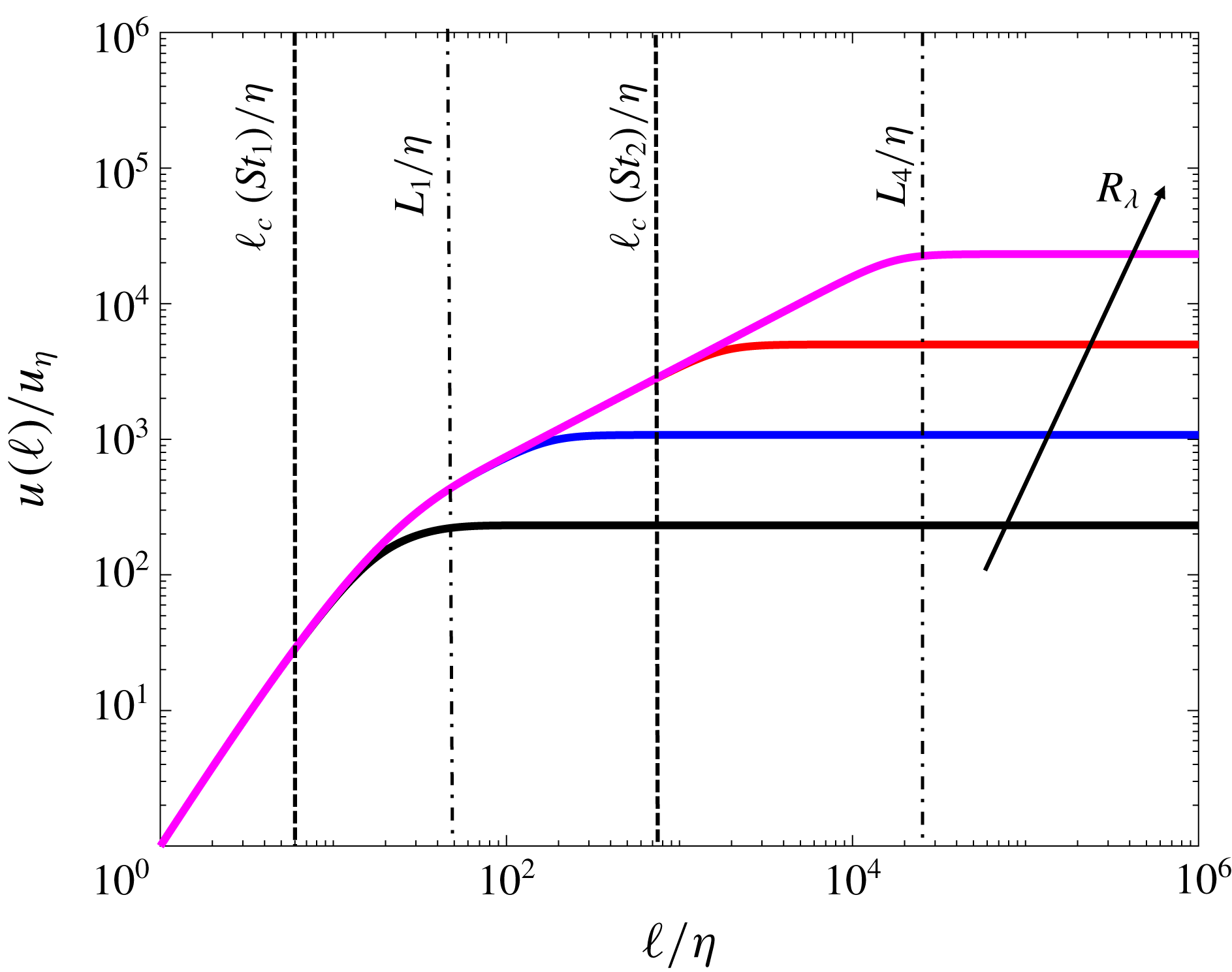In figure 1, we plot ${\mathcal{U}}(\ell )/u_{\unicode[STIX]{x1D702}}$ for four different values of $R_{\unicode[STIX]{x1D706}}$ (these curves are plotted using the curve fit for ${\mathcal{U}}(\ell )$ in Zaichik & Alipchenkov (Reference Zaichik and Alipchenkov2009)), and we denote the integral length scales for these flows as $L_{1},L_{2},L_{3},L_{4}$ , where $L_{1}<L_{2}<L_{3}<L_{4}$ (we assume $\unicode[STIX]{x1D702}$ is the same for each flow for simplicity of the discussion). Also indicated using dashed lines are two values of $\ell _{c}(St)$ corresponding to Stokes numbers $St_{1}$ and $St_{2}$ where $St_{1}<St_{2}$ so that $\ell _{c}(St_{1})<\ell _{c}(St_{2})$ . An important point is that when normalized by the Kolmogorov scales, ${\mathcal{U}}(\ell )$ is independent of $R_{\unicode[STIX]{x1D706}}$ when $\ell <L_{1}$ . Indeed a consequence of K41 is that when considering any two turbulent flows, ${\mathcal{U}}(\ell )/u_{\unicode[STIX]{x1D702}}$ will be independent of $R_{\unicode[STIX]{x1D706}}$ up to scales where $\ell$ is of the order of the integral length scale of the flow that has the smallest $R_{\unicode[STIX]{x1D706}}$ .

Now, let us consider how $\langle u_{z}(\boldsymbol{x}^{p}(t),t)\rangle /u_{\unicode[STIX]{x1D702}}$ would vary across these four $R_{\unicode[STIX]{x1D706}}$ values for $St_{1}$ and $St_{2}$ . For $St_{1}$ , since $\ell _{c}(St_{1})<L_{1}$ then $\langle u_{z}(\boldsymbol{x}^{p}(t),t)\rangle /u_{\unicode[STIX]{x1D702}}$ should be independent of $R_{\unicode[STIX]{x1D706}}$ since ${\mathcal{U}}(\ell )/u_{\unicode[STIX]{x1D702}}$ is the same for each of the flows until $\ell \geqslant L_{1}$ . On the other hand, for $St_{2}$ , $\langle u_{z}(\boldsymbol{x}^{p}(t),t)\rangle /u_{\unicode[STIX]{x1D702}}$ will differ for the smallest two values of $R_{\unicode[STIX]{x1D706}}$ since $\ell _{c}(St_{2})>L_{2}$ . However, for the largest two values of $R_{\unicode[STIX]{x1D706}}$ , $\langle u_{z}(\boldsymbol{x}^{p}(t),t)\rangle /u_{\unicode[STIX]{x1D702}}$ should be the same since $\ell _{c}(St_{2})<L_{3}$ . In other words, the $R_{\unicode[STIX]{x1D706}}$ dependence of $\langle u_{z}(\boldsymbol{x}^{p}(t),t)\rangle /u_{\unicode[STIX]{x1D702}}$ for $St_{2}$ will saturate once the integral length scale of the flow, $L(R_{\unicode[STIX]{x1D706}})$ , exceeds $\ell _{c}(St_{2})$ .

More generally, $\langle u_{z}(\boldsymbol{x}^{p}(t),t)\rangle /u_{\unicode[STIX]{x1D702}}$ will only depend on $R_{\unicode[STIX]{x1D706}}$ while $\ell _{c}(St)>L(R_{\unicode[STIX]{x1D706}})$ . For finite $St$ , $\ell _{c}(St)$ is always finite, and therefore for $R_{\unicode[STIX]{x1D706}}\rightarrow \infty$ , the $R_{\unicode[STIX]{x1D706}}$ dependence of $\langle u_{z}(\boldsymbol{x}^{p}(t),t)\rangle /u_{\unicode[STIX]{x1D702}}$ will always saturate for all finite $St$ .

Figure 1.

Plot to illustrate how $\ell _{c}(St)$ determines the $R_{\unicode[STIX]{x1D706}}$ dependence of $\langle u_{z}(\boldsymbol{x}^{p}(t),t)\rangle$ . The values of $R_{\unicode[STIX]{x1D706}}$ shown correspond to $R_{\unicode[STIX]{x1D706}}=[29,133,615,2854]$ .

3.1 DNS details

Our DNS dataset is identical to that in Ireland, Bragg & Collins (Reference Ireland, Bragg and Collins2016a ), Ireland et al. (Reference Ireland, Bragg and Collins2016b ), and we therefore refer the reader to that paper for the details of the DNS. Here we just give a brief summary. We perform a pseudo-spectral DNS of isotropic turbulence on a three-dimensional triperiodic cube of length ${\mathcal{L}}$ with $N^{3}$ grid points. The Navier–Stokes equation for an incompressible fluid was solved, with the pressure term eliminated using the divergence-free condition for the velocity field.

(3.1) $$\begin{eqnarray}\displaystyle & \displaystyle \unicode[STIX]{x1D735}\boldsymbol{\cdot }\boldsymbol{u}=0, & \displaystyle\end{eqnarray}$$

(3.2) $$\begin{eqnarray}\displaystyle & \displaystyle \frac{\unicode[STIX]{x2202}\boldsymbol{u}}{\unicode[STIX]{x2202}t}+\unicode[STIX]{x1D74E}\times \boldsymbol{u}+\unicode[STIX]{x1D735}\left(\frac{P}{\unicode[STIX]{x1D70C}_{f}}+\frac{u^{2}}{2}\right)=\unicode[STIX]{x1D708}\unicode[STIX]{x1D6FB}^{2}\boldsymbol{u}+\boldsymbol{f}, & \displaystyle\end{eqnarray}$$

where $\boldsymbol{u}$ is the fluid velocity, $\unicode[STIX]{x1D74E}$ is the vorticity, $P$ is the pressure, $\unicode[STIX]{x1D70C}_{f}$ is the fluid density, $\unicode[STIX]{x1D708}$ is the kinematic viscosity and $\boldsymbol{f}$ is a large scale forcing term that is added to make the flow field statistically stationary. Deterministic forcing was applied to wavenumbers with magnitude $k=\sqrt{2}$ . A detailed description of the numerical methods used can be found in Ireland et al. (Reference Ireland, Vaithianathan, Sukheswalla, Ray and Collins2013). The gravity term in the Navier–Stokes equation is precisely cancelled by the mean pressure gradient and so it has no dynamical consequence on the turbulent flow field. When using periodic boundary conditions, particles can artificially re-encounter the same large eddy as they are periodically looped through the domain, if the time it takes the settling particles to traverse the distance ${\mathcal{L}}$ is smaller than the large-eddy turnover time, i.e. if ${\mathcal{L}}/St\unicode[STIX]{x1D70F}_{\unicode[STIX]{x1D702}}g<O(\unicode[STIX]{x1D70F}_{L})$ . In all of our simulations, the domain lengths ${\mathcal{L}}$ are chosen to satisfy ${\mathcal{L}}/St\unicode[STIX]{x1D70F}_{\unicode[STIX]{x1D702}}g>\unicode[STIX]{x1D70F}_{L}$ , thereby suppressing the artificial periodicity effects for settling particles (a systematic study of this was presented in Ireland et al. (Reference Ireland, Bragg and Collins2016b )).

In order to analyse the same dynamical system we considered in the theory, we track inertial particles governed by (2.1), where particles are acted upon by both gravity and linear drag force. We assume that the particle loading is dilute and hence interparticle interactions and two-way coupling can be neglected (Elghobashi & Truesdell Reference Elghobashi and Truesdell1993; Sundaram & Collins Reference Sundaram and Collins1997). An eight-point B-spline interpolation scheme (with $C^{6}$ continuity) based on the algorithm in van Hinsberg et al. (Reference van Hinsberg, Thije Boonkkamp, Toschi and Clercx2012) was used to compute the fluid velocity at the particle position, $u(\boldsymbol{x}^{p}(t),t)$ . We consider $R_{\unicode[STIX]{x1D706}}=90,230$ and $398$ (note that we refer to the simulations with $R_{\unicode[STIX]{x1D706}}=224,230,237$ nominally as having $R_{\unicode[STIX]{x1D706}}\approx 230$ since they differ only due to statistical fluctuations, but correspond to the same $\unicode[STIX]{x1D708}$ ) and two $Fr$ that are representative of the conditions in clouds, $Fr=0.052$ for a cumulus clouds and $Fr=0.3$ for a strongly turbulent cumulonimbus cloud (see Ireland et al. Reference Ireland, Bragg and Collins2016b ). Fourteen different particle classes are simulated with $St\in [0,2]$ . 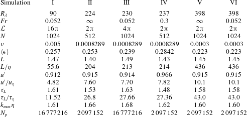Details of the simulations are given in table 1. Note that the data for $R_{\unicode[STIX]{x1D706}}=237$ and $Fr=0.3$ are from Momenifar, Dhariwal & Bragg (Reference Momenifar, Dhariwal and Bragg2018), while the rest are from Ireland et al. (Reference Ireland, Bragg and Collins2016a ,Reference Ireland, Bragg and Collins b ).

Table 1.

Flow parameters in DNS of isotropic turbulence where all dimensional parameters are in arbitrary units and all statistics are averaged over the duration of the run ( $T$ ). $R_{\unicode[STIX]{x1D706}}\equiv u^{\prime }\unicode[STIX]{x1D706}/\unicode[STIX]{x1D708}\equiv 2k/\sqrt{5/3\unicode[STIX]{x1D708}\langle \unicode[STIX]{x1D716}\rangle }$ is the Taylor microscale Reynolds number, $Fr$ is the Froude number, $\unicode[STIX]{x1D706}$ is the Taylor microscale, ${\mathcal{L}}$ is the domain size, $N$ is the number of grid points in each direction, $\unicode[STIX]{x1D708}$ is the fluid kinematic viscosity, $\langle \unicode[STIX]{x1D716}\rangle \equiv 2\unicode[STIX]{x1D708}\int _{0}^{\unicode[STIX]{x1D705}_{max}}\unicode[STIX]{x1D705}^{2}E(\unicode[STIX]{x1D705})\,\text{d}\unicode[STIX]{x1D705}$ is the mean turbulent kinetic energy dissipation rate, $\unicode[STIX]{x1D705}$ is the wavenumber in Fourier space, $E$ is the energy spectrum, $L\equiv (3\unicode[STIX]{x03C0}/2k)(\int _{0}^{\unicode[STIX]{x1D705}_{max}}(E(\unicode[STIX]{x1D705})/\unicode[STIX]{x1D705})\,\text{d}\unicode[STIX]{x1D705})$ is the integral length scale, $\unicode[STIX]{x1D702}\equiv (\unicode[STIX]{x1D708}^{3}/\langle \unicode[STIX]{x1D716}\rangle )^{1/4}$ is the Kolmogorov length scale, $u^{\prime }\equiv \sqrt{2k/3}$ is the r.m.s. of fluctuating fluid velocity, $k$ is the turbulent kinetic energy, $u_{\unicode[STIX]{x1D702}}\equiv (\langle \unicode[STIX]{x1D716}\rangle \unicode[STIX]{x1D708})^{3/4}$ is the Kolmogorov velocity scale, $\unicode[STIX]{x1D70F}_{L}\equiv L/u^{\prime }$ is the large-eddy turnover time, $\unicode[STIX]{x1D70F}_{\unicode[STIX]{x1D702}}\equiv \sqrt{\unicode[STIX]{x1D708}/\langle \unicode[STIX]{x1D716}\rangle }$ is the Kolmogorov time scale, $k_{max}=\sqrt{2N/3}$ is the maximum resolved wavenumber and $N_{p}$ is the number of particles per Stokes number used in the simulation. The grid spacing is kept constant as the domain size is increased, and so the small scale resolution, $k_{max}\unicode[STIX]{x1D702}$ , is approximately constant between the different domain sizes. The viscosity and forcing parameters were kept the same when increasing domain size, and thus both small scale and large scale flow parameters are held approximately constant.

3.2 Testing methodology

It would be very difficult to directly test (2.19) owing to the practical difficulty in constructing the field $\boldsymbol{{\mathcal{V}}}^{\prime }(\boldsymbol{x},t)$ (and a simple evolution equation for $\boldsymbol{{\mathcal{V}}}^{\prime }(\boldsymbol{x},t)$ is not available). However, the insights and predictions from the theoretical analysis can be tested by computing $\langle u_{z}^{\prime }(\boldsymbol{x}^{p}(t),t)\rangle$ for various coarse-graining length scales, and analysing how the coarse graining affects the results for varying $St,R_{\unicode[STIX]{x1D706}}$ and $Fr$ . Strictly speaking, $\langle u_{z}^{\prime }(\boldsymbol{x}^{p}(t),t)\rangle$ does not actually correspond to (2.19), but rather corresponds to (2.19) with $\unicode[STIX]{x1D735}\boldsymbol{\cdot }\boldsymbol{{\mathcal{V}}}^{\prime }$ replaced by $\unicode[STIX]{x1D735}\boldsymbol{\cdot }\boldsymbol{{\mathcal{V}}}$ . However, according to the arguments and definitions leading to (2.19), these two quantities are asymptotically equivalent since the coarse-graining length scale $\ell _{c}$ is defined in such a way that $\unicode[STIX]{x1D735}\boldsymbol{\cdot }\boldsymbol{{\mathcal{V}}}^{\prime }\approx \unicode[STIX]{x1D735}\boldsymbol{\cdot }\boldsymbol{{\mathcal{V}}}$ since $|\unicode[STIX]{x1D735}\boldsymbol{\cdot }\widetilde{\boldsymbol{{\mathcal{V}}}}|\lll |\unicode[STIX]{x1D735}\boldsymbol{\cdot }\boldsymbol{{\mathcal{V}}}^{\prime }|$ . Therefore, comparing $\langle u_{z}^{\prime }(\boldsymbol{x}^{p}(t),t)\rangle$ with the implications and predictions following from (2.19) is appropriate.

To take full advantage of our existing large database on inertial particle motion in isotropic turbulence (see Ireland et al. Reference Ireland, Bragg and Collins2016a ,Reference Ireland, Bragg and Collins b ), we compute $\langle u_{z}^{\prime }(\boldsymbol{x}^{p}(t),t)\rangle$ from our existing DNS data via postprocessing. To do this we take our DNS data for $u_{z}(\boldsymbol{x},t)$ and the particle positions $\boldsymbol{x}^{p}(t)$ at a number of different times, for multiple $St$ , $R_{\unicode[STIX]{x1D706}}$ and $Fr$ . We then apply a sharp spectral cutoff at wavenumber $k_{F}$ to $u_{z}(\boldsymbol{x},t)$ , and from this obtain the subgrid field through

(3.3) $$\begin{eqnarray}u_{z}^{\prime }(\boldsymbol{x},t)\equiv u_{z}(\boldsymbol{x},t)-\widetilde{u}_{z}(\boldsymbol{x},t)=\mathop{\sum }_{\Vert \boldsymbol{k}\Vert >k_{F}}\hat{u} _{z}(\boldsymbol{k},t)\text{e}^{\text{i}\boldsymbol{k}\boldsymbol{\cdot }\boldsymbol{x}},\end{eqnarray}$$

where here and throughout, $\widetilde{(\cdot )}$ denotes the coarse-grained field, while $(\cdot )^{\prime }$ denotes the subgrid field. We then interpolate $u_{z}^{\prime }(\boldsymbol{x},t)$ to the positions of inertial particles $\boldsymbol{x}^{p}(t)$ using an eighth-order B-spline interpolation scheme to obtain $u_{z}^{\prime }(\boldsymbol{x}^{p}(t),t)$ . The values of $u_{z}^{\prime }(\boldsymbol{x}^{p}(t),t)$ are then averaged over all the particles (with a given $St$ ) and over multiple times to obtain $\langle u_{z}^{\prime }(\boldsymbol{x}^{p}(t),t)\rangle$ . This process is then repeated for multiple $k_{c}$ in order to examine the effect of the coarse graining and how its effect depends on $St,R_{\unicode[STIX]{x1D706}}$ and $Fr$ . In order to relate the spectral cutoff wavenumber $k_{F}$ to a physical space filtering scale we define $\ell _{F}\equiv 2\unicode[STIX]{x03C0}/k_{F}$ (Eyink & Aluie Reference Eyink and Aluie2009).

By considering the results of $\langle u_{z}^{\prime }(\boldsymbol{x}^{p}(t),t)\rangle$ for various $St,\ell _{F},Fr$ and $R_{\unicode[STIX]{x1D706}}$ and comparing them with those for $\langle u_{z}(\boldsymbol{x}^{p}(t),t)\rangle$ , we can test the predictions of the theory regarding which flow scales contribute to $\langle u_{z}(\boldsymbol{x}^{p}(t),t)\rangle$ .

4.1 The scales of motion that influence the particle settling speed

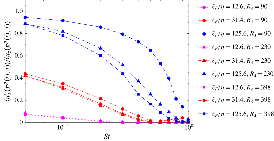
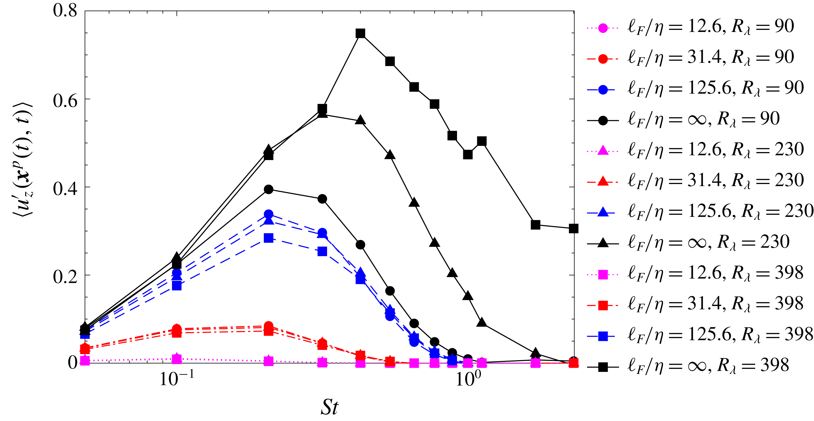
The theoretical analysis predicts that the range of scales that contribute to $\langle u_{z}(\boldsymbol{x}^{p}(t),t)\rangle$ should monotonically increase as $St$ increases. To test this prediction, in figure 2, we plot the ratio $\langle u_{z}^{\prime }(\boldsymbol{x}^{p}(t),t)\rangle /\langle u_{z}(\boldsymbol{x}^{p}(t),t)\rangle$ for various filtering length scales $\ell _{F}$ , and various $R_{\unicode[STIX]{x1D706}}$ . For $St\lll 1$ we would have $\ell _{c}(St)=O(\unicode[STIX]{x1D702})$ , and so filtering out scales $\ell _{F}>O(\unicode[STIX]{x1D702})$ would have little effect, since the particle settling speed is only affected by the scales less than $\ell _{c}(St)$ . Hence, for $St\lll 1$ , we expect $\langle u_{z}^{\prime }(\boldsymbol{x}^{p}(t),t)\rangle /\langle u_{z}(\boldsymbol{x}^{p}(t),t)\rangle \approx 1$ . On the other hand, for $St=O(1)$ we would have $\ell _{c}(St)>O(\unicode[STIX]{x1D702})$ , and so filtering out scales $\ell _{F}>O(\unicode[STIX]{x1D702})$ would have a strong effect, since these scales make a strong contribution to the particle settling speed. Hence, for $St=O(1)$ , we expect $\langle u_{z}^{\prime }(\boldsymbol{x}^{p}(t),t)\rangle /\langle u_{z}(\boldsymbol{x}^{p}(t),t)\rangle \ll 1$ . More generally, the prediction is that for a given $\ell _{F}$ , $\langle u_{z}^{\prime }(\boldsymbol{x}^{p}(t),t)\rangle /\langle u_{z}(\boldsymbol{x}^{p}(t),t)\rangle$ should decrease with increasing $St$ , reflecting the fact that $\langle u_{z}(\boldsymbol{x}^{p}(t),t)\rangle$ is affected by increasingly larger scales as $St$ is increased. The results in figure 2 confirm this prediction. They also reveal how sensitive $\langle u_{z}(\boldsymbol{x}^{p}(t),t)\rangle$ is to scales $\ell \gg \unicode[STIX]{x1D702}$ , even when $St=O(0.1)$ , which is quite surprising.

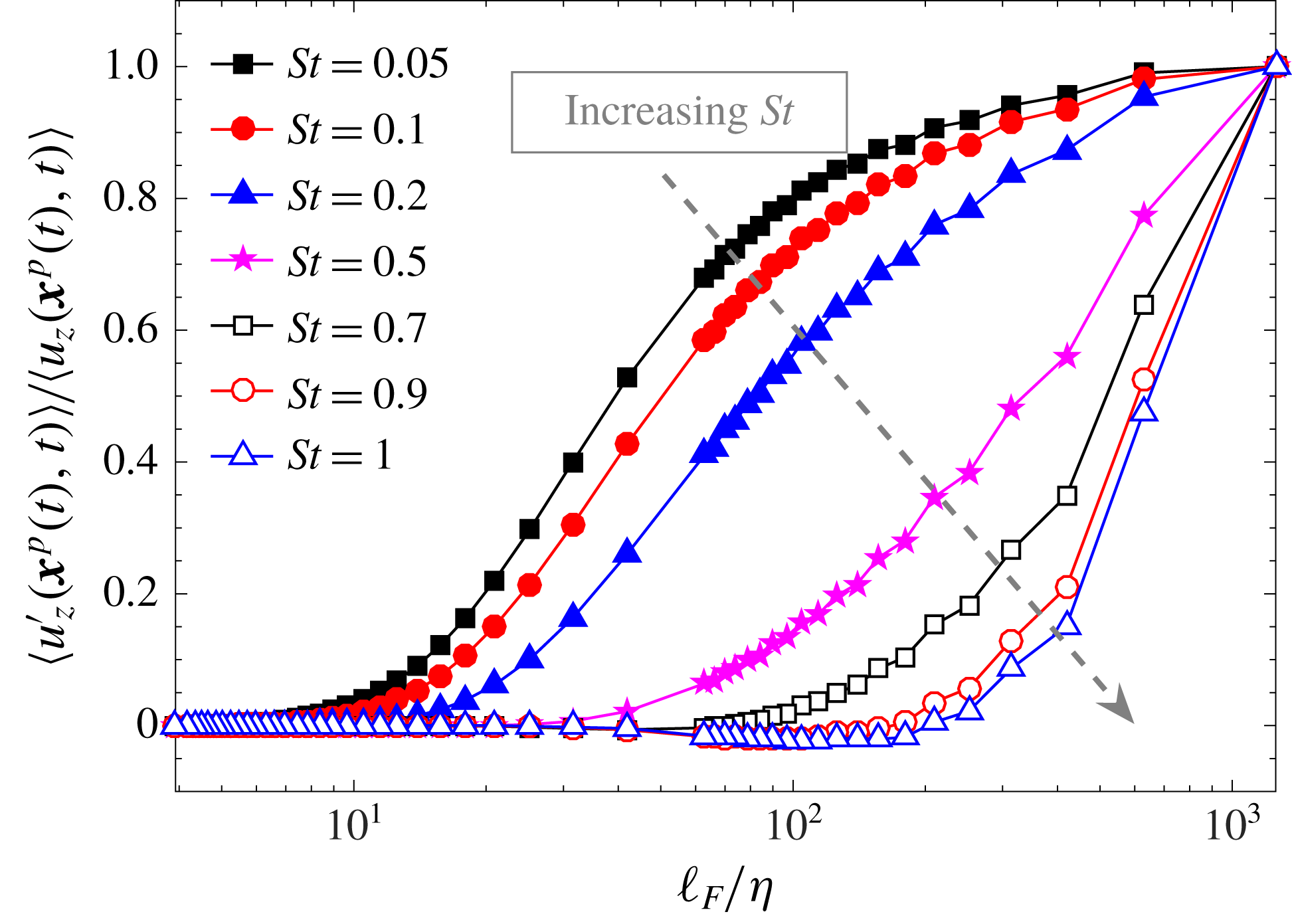
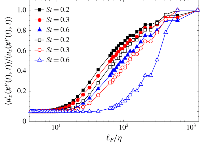
To further illustrate this behaviour, in figure 3, we plot $\langle u_{z}^{\prime }(\boldsymbol{x}^{p}(t),t)\rangle /\langle u_{z}(\boldsymbol{x}^{p}(t),t)\rangle$ as a function of $\ell _{F}/\unicode[STIX]{x1D702}$ for various $St$ . For $St\lesssim 0.2$ we clearly see that as $\ell _{F}$ is increased, $\langle u_{z}^{\prime }(\boldsymbol{x}^{p}(t),t)\rangle$ approaches a constant value, implying that there do indeed exist scales beyond a certain size that have a negligible effect on the particle settling velocity, as predicted by the theory. However, for $St=O(1)$ , we do not see such an asymptote, and their settling velocity is significantly affected by the largest scales in the flow. In order to understand why this is the case, we will now estimate $\ell _{c}(St)$ .

Figure 2.

DNS results for $\langle u_{z}^{\prime }(\boldsymbol{x}^{p}(t),t)\rangle /\langle u_{z}(\boldsymbol{x}^{p}(t),t)\rangle$ as a function of $St$ , for $Fr=0.052$ , and for various filtering lengths $\ell _{F}/\unicode[STIX]{x1D702}$ . The circles correspond to $R_{\unicode[STIX]{x1D706}}=90$ , the triangles to $R_{\unicode[STIX]{x1D706}}\approx 230$ and the squares to $R_{\unicode[STIX]{x1D706}}=398$ . The dashed lines correspond to $\ell _{F}/\unicode[STIX]{x1D702}=125.6$ , the dash-dot lines to $\ell _{F}/\unicode[STIX]{x1D702}=31.4$ , and the dotted lines to $\ell _{F}/\unicode[STIX]{x1D702}=12.6$ .

Figure 3.

DNS data for $\langle u_{z}^{\prime }(\boldsymbol{x}^{p}(t),t)\rangle /\langle u_{z}(\boldsymbol{x}^{p}(t),t)\rangle$ as a function of $\ell _{F}/\unicode[STIX]{x1D702}$ for different $St$ , and $Fr=0.052$ , $R_{\unicode[STIX]{x1D706}}=398$ .

Figure 4.

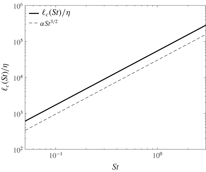
Plot illustrating how $\ell _{c}(St)/\unicode[STIX]{x1D702}$ grows with $St$ .

Recall that in the derivation of our theoretical result we prescribed the parameter $\unicode[STIX]{x1D6FE}$ to have the asymptotic value $\unicode[STIX]{x1D6FE}\lll 1$ . However, we may estimate a value for $\unicode[STIX]{x1D6FE}$ from our DNS. To do this, we note that for $St=0.05$ , $\langle u_{z}^{\prime }(\boldsymbol{x}^{p}(t),t)\rangle /\langle u_{z}(\boldsymbol{x}^{p}(t),t)\rangle \approx 1$ for $\ell _{F}/\unicode[STIX]{x1D702}\gtrsim 600$ and hence $\ell _{c}(St=0.05)\approx 600\unicode[STIX]{x1D702}$ . Then using the K41 result discussed earlier, $\ell _{c}(St)\sim \unicode[STIX]{x1D702}(St/\unicode[STIX]{x1D6FE})^{3/2}$ and using $\ell _{c}(St=0.05)\approx 600\unicode[STIX]{x1D702}$ , we obtain the estimate $\unicode[STIX]{x1D6FE}\approx 7\times 10^{-4}$ . Using this value, in figure 4 we plot $\ell _{c}(St)\sim \unicode[STIX]{x1D702}(St/\unicode[STIX]{x1D6FE})^{3/2}$ , where we have taken $R_{\unicode[STIX]{x1D706}}\rightarrow \infty$ so that the inertial range scaling $\ell _{c}(St)\sim \unicode[STIX]{x1D702}(St/\unicode[STIX]{x1D6FE})^{3/2}$ applies for all $St\geqslant 0.05$ . Using this estimated behaviour we find that for $St=1$ , $\ell _{c}(St)/\unicode[STIX]{x1D702}\approx 5.4\times 10^{4}$ . In our DNS at $R_{\unicode[STIX]{x1D706}}=398$ , the ratio of the integral length scale $L$ to $\unicode[STIX]{x1D702}$ is $L/\unicode[STIX]{x1D702}=4.3\times 10^{2}$ which is two orders of magnitude smaller than $\ell _{c}(St)/\unicode[STIX]{x1D702}$ for $St=1$ . This then explains why in our DNS we do not observe a saturation of $\langle u_{z}^{\prime }(\boldsymbol{x}^{p}(t),t)\rangle /\langle u_{z}(\boldsymbol{x}^{p}(t),t)\rangle$ for $St=O(1)$ as $\ell _{F}$ is increased. An important conclusion that follows from this is that while the settling speed of particles is dominated by a restricted range of scales, namely scales of size less than $\ell _{c}(St)$ , this range can actually be quite large. Indeed, figure 4, and the results in figure 3 indicate that even for $St=0.1$ , $\ell _{c}(St)/\unicode[STIX]{x1D702}\approx 1.7\times 10^{3}$ such that their settling speeds are affected by scales much larger than those in the dissipation range.

These findings also explain why in many previous numerical and experimental studies, it was found that $\langle u_{z}(\boldsymbol{x}^{p}(t),t)\rangle$ had a strong dependence on $u^{\prime }$ , the large scale fluid velocity scale. We have argued that on theoretical grounds, $\langle u_{z}(\boldsymbol{x}^{p}(t),t)\rangle$ cannot be characterized by a single flow scale since the range of scales contributing to $\langle u_{z}(\boldsymbol{x}^{p}(t),t)\rangle$ depends on $St$ . However, in these previous works $R_{\unicode[STIX]{x1D706}}$ was sufficiently small so that the particle settling speeds were significantly affected by all scales, and as a result $\langle u_{z}(\boldsymbol{x}^{p}(t),t)\rangle$ was found to have a strong dependence on $u^{\prime }$ . In contrast, in natural flows where $R_{\unicode[STIX]{x1D706}}$ is much larger, this would not be the case. In the atmosphere, typical values are $\unicode[STIX]{x1D702}=O(mm)$ and $L=O(100~\text{m})$ (Shaw Reference Shaw2003; Grabowski & Wang Reference Grabowski and Wang2013), and together with the results in figure 4 this implies we would have, for example, $\ell _{c}(St=0.1)\approx 1.7~\text{m}$ and $\ell _{c}(St=1)\approx 54~\text{m}$ . Consequently, for $St\leqslant 1$ , the large scale fluid velocities in the atmosphere, characterized by $u^{\prime }$ , would play no role in the particle settling. Nevertheless, the estimate $\ell _{c}(St=1)\approx 54~\text{m}$ shows that the range of atmospheric flow scales that may contribute to the enhanced settling speeds due to turbulence is quite large. This means that for $St=O(1)$ , particle settling in the atmosphere may be strongly influenced by non-ideal effects such as flow inhomogeneity, anisotropy and stratification (noting that the Ozmidov scale is greater than or equal to $O(m)$ in the atmosphere (Riley & Lindborg Reference Riley and Lindborg2012)).

So far we have emphasized that as $St$ is increased, larger scales contribute to the particle settling since $\ell _{c}(St)$ is a non-decreasing function of $St$ . However, in reality, as $St$ is increased, not only do larger scales contribute to the particle settling, but smaller scales begin to contribute less. This is because the preferential sweeping effect at any scale is only effective when $St_{\ell }\not \lll 1$ and $St_{\ell }\not \ggg 1$ . Let us define $\widehat{\ell }_{c}(St)$ as the scale below which the preferential sweeping mechanism is not effective, so that scales $\ell <\widehat{\ell }_{c}(St)$ correspond to scales at which $St_{\ell }\ggg 1$ . Then, the scales at which the preferential sweeping mechanism would operate are $\widehat{\ell }_{c}(St)\leqslant \ell <\ell _{c}(St)$ , and both $\widehat{\ell }_{c}(St)$ and $\ell _{c}(St)$ are non-decreasing functions of $St$ . While our theoretical analysis could be extended to also include the lower limit scale $\widehat{\ell }_{c}(St)$ , we have chosen not to do so since it would render the theoretical result much more complicated. Furthermore, our principle concern in this paper is to understand the upper limit of the turbulent flow scales that contribute to the particle settling velocity in a turbulent flow, and this is given by $\ell _{c}(St)$ . Nevertheless, understanding the minimum flow scales affecting the settling process is key to the development of particle subgrid scale (SGS) models for LES of particles settling in turbulent flows. The effect of the smallest scales of the turbulence on particle settling speeds was investigated by Rosa & Pozorski (Reference Rosa and Pozorski2017) using DNS and their results showed that scales smaller than a certain size did not affect the particle settling speeds. Although their data do not provide enough information to determine exactly how this ‘cutoff scale’ depends on $St$ , their data are consistent with our theoretical prediction that $\widehat{\ell }_{c}(St)$ is a non-decreasing function of $St$ .

4.2 Influence of $R_{\unicode[STIX]{x1D706}}$ on the particle settling speed

As discussed in § 2.4.2, as $R_{\unicode[STIX]{x1D706}}$ is increased, the range of scales in the turbulent flow increases. According to our theoretical analysis, when $St\lll 1$ , $\ell _{c}(St)$ is small enough so that the particles are not influenced by the additional scales introduced by increasing $R_{\unicode[STIX]{x1D706}}$ . Consequently, $\langle u_{z}(\boldsymbol{x}^{p}(t),t)\rangle$ should not vary with $R_{\unicode[STIX]{x1D706}}$ for $St\lll 1$ . However, as $St$ is increased, so also does $\ell _{c}(St)$ , and for sufficiently large $St$ , this allows the particles to feel the effects of the additional flow scales introduced by increasing $R_{\unicode[STIX]{x1D706}}$ . As a result, $\langle u_{z}^{\prime }(\boldsymbol{x}^{p}(t),t)\rangle$ can depend on $R_{\unicode[STIX]{x1D706}}$ as $St$ is increased. The results in figure 5 confirm this picture and show that without filtering (i.e.  $\ell _{F}/\unicode[STIX]{x1D702}=\infty$ ), $\langle u_{z}^{\prime }(\boldsymbol{x}^{p}(t),t)\rangle =\langle u_{z}(\boldsymbol{x}^{p}(t),t)\rangle$ is significantly enhanced with increasing $R_{\unicode[STIX]{x1D706}}$ when $St\gtrsim 0.2$ , whereas it is almost insensitive to $R_{\unicode[STIX]{x1D706}}$ when $St\lesssim 0.1$ .

Figure 5.

DNS results for $\langle u_{z}^{\prime }(\boldsymbol{x}^{p}(t),t)\rangle$ as a function of $St$ , for $Fr=0.052$ , and for various filtering lengths $\ell _{F}/\unicode[STIX]{x1D702}$ . The circles correspond to $R_{\unicode[STIX]{x1D706}}=90$ , the triangles to $R_{\unicode[STIX]{x1D706}}\approx 230$ and the squares to $R_{\unicode[STIX]{x1D706}}=398$ . The solid lines correspond to $\ell _{F}/\unicode[STIX]{x1D702}=\infty$ , the dashed lines to $\ell _{F}/\unicode[STIX]{x1D702}=125.6$ , the dash-dot lines to $\ell _{F}/\unicode[STIX]{x1D702}=31.4$ and the dotted lines to $\ell _{F}/\unicode[STIX]{x1D702}=12.6$ .

The results in figure 5 also show that when scales larger than some finite $\ell _{F}/\unicode[STIX]{x1D702}$ are filtered out, so that the range of scales contained in $u_{z}^{\prime }$ is the same for each $R_{\unicode[STIX]{x1D706}}$ , the $R_{\unicode[STIX]{x1D706}}$ dependence of $\langle u_{z}^{\prime }(\boldsymbol{x}^{p}(t),t)\rangle$ is dramatically suppressed. Indeed, for $St\gtrsim 0.4$ the effect of $R_{\unicode[STIX]{x1D706}}$ is entirely suppressed for $\ell _{F}/\unicode[STIX]{x1D702}$ values considered. This confirms that the strong effect of $R_{\unicode[STIX]{x1D706}}$ on $\langle u_{z}(\boldsymbol{x}^{p}(t),t)\rangle$ is principally due to the enhanced range of scales available for the particles to preferentially sample as $R_{\unicode[STIX]{x1D706}}$ is increased. Recall that increasing $R_{\unicode[STIX]{x1D706}}$ leads to two distinct effects, namely an increased range of flow scales, and enhanced intermittency. While filtering eliminates the effect of the increased range of scales by removing scales greater than $\ell _{F}$ (so that each flow of differing $R_{\unicode[STIX]{x1D706}}$ has the same range of scales), the effect of enhanced intermittency still remains. It can be seen in figure 5 that for $\ell _{F}/\unicode[STIX]{x1D702}\leqslant 125.6$ , the curves collapse for $St\gtrsim 0.4$ , while there is a residual effect of $R_{\unicode[STIX]{x1D706}}$ for $St\lesssim 0.3$ , which must be due to intermittency. That the effect of intermittency is only apparent for small $St$ is consistent with previous works which show that the effect of flow intermittency on inertial particle motion in turbulence is mainly confined to small $St$ , while larger $St$ particles filter out the effects of intermittent fluctuations in the flow (Bec et al. Reference Bec, Biferale, Boffetta, Celani, Cencini, Lanotte, Musacchio and Toschi2006; Ayyalasomayajula, Warhaft & Collins Reference Ayyalasomayajula, Warhaft and Collins2008).

To observe the effect of $R_{\unicode[STIX]{x1D706}}$ more clearly, in figure 6, we plot ${\mathcal{A}}(R_{\unicode[STIX]{x1D706}},St)/{\mathcal{A}}(R_{\unicode[STIX]{x1D706}}=90,St)$ where ${\mathcal{A}}(R_{\unicode[STIX]{x1D706}},St)\equiv \langle u_{z}(\boldsymbol{x}^{p}(t),t)\rangle /u_{\unicode[STIX]{x1D702}}$ , as a function of $R_{\unicode[STIX]{x1D706}}$ and for different values of $St$ . In agreement with the theoretical analysis, as $St$ is increased, ${\mathcal{A}}(R_{\unicode[STIX]{x1D706}},St)/{\mathcal{A}}(R_{\unicode[STIX]{x1D706}}=90,St)$ becomes increasingly sensitive to $R_{\unicode[STIX]{x1D706}}$ . The analysis leads us to expect that for any $St$ , the ratio ${\mathcal{A}}(R_{\unicode[STIX]{x1D706}},St)/{\mathcal{A}}(R_{\unicode[STIX]{x1D706}}=90,St)$ will eventually saturate at sufficiently large $R_{\unicode[STIX]{x1D706}}$ and the $R_{\unicode[STIX]{x1D706}}$ at which saturation occurs would increase with $St$ . Our data are consistent with this, however, we do not have enough $R_{\unicode[STIX]{x1D706}}$ data points to be conclusive, and data at larger $R_{\unicode[STIX]{x1D706}}$ are required to observe the saturation for $St=O(1)$ . Again, this is because in order to observe the saturation we must consider values of $R_{\unicode[STIX]{x1D706}}$ for which $\ell _{c}(St)<L(R_{\unicode[STIX]{x1D706}})$ , and our DNS does not satisfy this for $R_{\unicode[STIX]{x1D706}}\leqslant 398$ and $St=O(1)$ .

Figure 6.

DNS results for ${\mathcal{A}}(R_{\unicode[STIX]{x1D706}},St)/{\mathcal{A}}(R_{\unicode[STIX]{x1D706}}=90,St)$ as a function of $R_{\unicode[STIX]{x1D706}}$ , for various $St$ , and for $Fr=0.052$ .

4.3 Influence of Froude number on the scales governing particle settling speeds

Another prediction of the theory is that for a given $St$ , as $Fr$ is decreased, $\ell _{c}(St)$ increases meaning that larger scales become responsible for the behaviour of $\langle u_{z}(\boldsymbol{x}^{p}(t),t)\rangle$ . In figure 7, we plot $\langle u_{z}^{\prime }(\boldsymbol{x}^{p}(t),t)\rangle$ for $Fr=0.3$ and $Fr=0.052$ , each at $R_{\unicode[STIX]{x1D706}}\approx 230$ . For $St\gtrsim 0.1$ , the results confirm the prediction, since they show that $\langle u_{z}(\boldsymbol{x}^{p}(t),t)\rangle$ is more strongly affected by filtering as $Fr$ is decreased, which is equivalent to saying that $\langle u_{z}(\boldsymbol{x}^{p}(t),t)\rangle$ is affected by increasingly larger scales as $Fr$ is decreased.

Figure 7.

DNS results for $\langle u_{z}^{\prime }(\boldsymbol{x}^{p}(t),t)\rangle /\langle u_{z}(\boldsymbol{x}^{p}(t),t)\rangle$ as a function of $St$ for $Fr=0.052$ (squares) and $Fr=0.3$ (circles), and $R_{\unicode[STIX]{x1D706}}\approx 230$ . The solid lines correspond to $\ell _{F}/\unicode[STIX]{x1D702}=125.6$ , the dashed lines to $\ell _{F}/\unicode[STIX]{x1D702}=31.4$ , and the dash-dot lines to $\ell _{F}/\unicode[STIX]{x1D702}=12.6$ .

Figure 8.

DNS data for $\langle u_{z}^{\prime }(\boldsymbol{x}^{p}(t),t)\rangle /\langle u_{z}(\boldsymbol{x}^{p}(t),t)\rangle$ as a function of $\ell _{F}/\unicode[STIX]{x1D702}$ for different $St$ , and $Fr=0.3$ (filled symbols), $Fr=0.052$ (open symbols), and $R_{\unicode[STIX]{x1D706}}\approx 230$ .

To show this more clearly, in figure 8 we plot the ratio $\langle u_{z}^{\prime }(\boldsymbol{x}^{p}(t),t)\rangle /\langle u_{z}(\boldsymbol{x}^{p}(t),t)\rangle$ as a function of $\ell _{F}/\unicode[STIX]{x1D702}$ , for different $Fr$ , $St$ and for $R_{\unicode[STIX]{x1D706}}\approx 230$ . The results show that as $Fr$ is decreased, the ratio decreases for a given $St$ and $\ell _{F}/\unicode[STIX]{x1D702}$ . This confirms the prediction of the theory as it indicates that as $Fr$ is decreased, larger scales become responsible for the enhanced particle settling speeds due to turbulence. This could also explain the increased cluster size (determined by Voronoi tessellation) in the presence of gravity observed by Baker et al. (Reference Baker, Frankel, Mani and Coletti2017). In particular, as the particles settle faster due to gravity, the scales at which the clustering mechanisms (such as the preferential sampling of the filtered velocity gradient field, see Bragg et al. (Reference Bragg, Ireland and Collins2015)) become active move to larger scales.

4.4 Scale dependence of preferential sweeping

So far, we have tested the predictions following from our theoretical analysis regarding the scales that contribute to enhanced particles settling speeds in turbulence. We now turn to consider in more detail the multiscale nature of the preferential sweeping mechanism. Recall that the preferential sweeping mechanism involves the idea that the enhanced particle settling is associated with the tendency of inertial particles to preferentially sample the flow by preferring paths around the downward side of vortices. However, according to our theoretical analysis this preferential sweeping can only take place at scales $\ell <\ell _{c}(St)$ , such that the preferential sweeping mechanism is multiscale in general, and does not only involve the small scales as in the $St\ll 1$ analysis of Maxey (Reference Maxey1987).

A traditional way to consider preferential sampling of the flow by inertial particles is to consider ${\mathcal{Q}}^{p}(t)\equiv {\mathcal{S}}^{2}(\boldsymbol{x}^{p}(t),t)-{\mathcal{R}}^{2}(\boldsymbol{x}^{p}(t),t)$ , where ${\mathcal{S}}^{2}$ and ${\mathcal{R}}^{2}$ are the second invariants of the strain-rate $\boldsymbol{{\mathcal{S}}}\equiv (\unicode[STIX]{x1D735}\boldsymbol{u}+\unicode[STIX]{x1D735}\boldsymbol{u}^{\top })/2$ and rotation-rate $\boldsymbol{{\mathcal{R}}}\equiv (\unicode[STIX]{x1D735}\boldsymbol{u}-\unicode[STIX]{x1D735}\boldsymbol{u}^{\top })/2$ tensors, respectively. Comparing the statistics of ${\mathcal{Q}}^{p}(t)$ along fluid and inertial particle trajectories provides a clear way to consider preferential sampling since their statistics can only differ if the inertial particles are both non-uniformly distributed, and if their distribution is correlated to the local flow, i.e. if they exhibit preferential concentration. However, in order to consider how the particles preferential sample the flow at different scales we must instead consider the coarse-grained quantity $\widetilde{{\mathcal{Q}}}^{p}(t)\equiv \widetilde{{\mathcal{S}}}^{2}(\boldsymbol{x}^{p}(t),t)-\widetilde{{\mathcal{R}}}^{2}(\boldsymbol{x}^{p}(t),t)$ , where $\widetilde{{\mathcal{S}}}^{2}\equiv \widetilde{\boldsymbol{{\mathcal{S}}}}\boldsymbol{ : }\widetilde{\boldsymbol{{\mathcal{S}}}}$ , $\widetilde{{\mathcal{R}}}^{2}\equiv \widetilde{\boldsymbol{{\mathcal{R}}}}\boldsymbol{ : }\widetilde{\boldsymbol{{\mathcal{R}}}}$ and $\widetilde{\boldsymbol{{\mathcal{S}}}}$ , $\widetilde{\boldsymbol{{\mathcal{R}}}}$ denote $\boldsymbol{{\mathcal{S}}}$ , $\boldsymbol{{\mathcal{R}}}$ coarse grained on the scale $\ell _{F}$ .

Figure 9.

DNS data for ${\mathcal{P}}(\widetilde{{\mathcal{Q}}},t)$ and different $St$ . Panels (a,b) are for $\ell _{F}/\unicode[STIX]{x1D702}=0$ , while panels (c,d) are for $\ell _{F}/\unicode[STIX]{x1D702}=66.1$ . Panels (a,c) are for $Fr=\infty$ , while panels (b,d) are for $Fr=0.052$ .

In figure 9, we plot the PDF of $\widetilde{{\mathcal{Q}}}^{p}(t)$ , namely

(4.1) $$\begin{eqnarray}{\mathcal{P}}(\widetilde{{\mathcal{Q}}},t)\equiv \langle \unicode[STIX]{x1D6FF}(\widetilde{{\mathcal{Q}}}^{p}(t)-\widetilde{{\mathcal{Q}}})\rangle ,\end{eqnarray}$$

where $\widetilde{{\mathcal{Q}}}$ is the sample-space variable. The results are shown for $R_{\unicode[STIX]{x1D706}}=398$ , $Fr=\infty$ and $Fr=0.052$ , and for different $St$ and $\ell _{F}/\unicode[STIX]{x1D702}$ . The results show, as expected, that the role of $St$ is different at different scales, which is because the behaviour of ${\mathcal{P}}(\widetilde{{\mathcal{Q}}},t)$ at any scale depends upon $St_{\ell }$ , not $St$ . The results also show the strong effect of gravity on the preferential sampling, which is to suppress it. For example, in figure 9(c), corresponding to the no gravity case, we see that preferential sampling is strongest for $St=1$ . However, the results in in figure 9(d) show that when gravity is active, the preferential sampling for $St=1$ is very weak. The suppression of preferential sampling due to gravity at any scale is because as $Fr$ is decreased, the particles fall through the flow faster, which in turn reduces the interaction time between the particles and flow eddies, thereby causing the centrifuging mechanism to be less efficient. We emphasize, however, that this does not mean that their clustering is diminished by gravity. Indeed it has been shown using DNS that for $St\gtrsim 1$ , clustering is actually enhanced by gravity (Bec et al. Reference Bec, Homann and Ray2014; Ireland et al. Reference Ireland, Bragg and Collins2016b ). This is a reflection of the distinction between clustering and preferential concentration and the mechanisms responsible for each, as discussed in § 2.2. The subtle, but important point is that it is preferential concentration/sampling that determines the enhanced particle settling due to turbulence, and not clustering per se (see § 2.2).

Figure 10.

DNS data for $\langle \widetilde{{\mathcal{Q}}}^{p}(t)\rangle /\sqrt{\langle [\widetilde{{\mathcal{Q}}}^{p}(t)]^{2}\rangle -\langle \widetilde{{\mathcal{Q}}}^{p}(t)\rangle ^{2}}$ as a function of $St$ for different $\ell _{F}/\unicode[STIX]{x1D702}$ , for $Fr=\infty$ (filled symbols) and $Fr=0.052$ (open symbols), and $R_{\unicode[STIX]{x1D706}}=398$ .

Further quantitative information concerning the preferential sampling may be obtained by considering the quantity

(4.2) $$\begin{eqnarray}\langle \widetilde{{\mathcal{Q}}}^{p}(t)\rangle /\sqrt{\langle [\widetilde{{\mathcal{Q}}}^{p}(t)]^{2}\rangle -\langle \widetilde{{\mathcal{Q}}}^{p}(t)\rangle ^{2}}.\end{eqnarray}$$

For homogeneous turbulence, this quantity is zero when measured along the trajectories of particles that do not preferentially sample the flow. The results in figure 10 show that with or without gravity, the maximum value for this quantity weakens as $\ell _{F}$ is increased. This then implies that the maximum preferential sampling decreases with increasing scale. As $\ell _{F}$ is increased, we also see that the peak value of the curve shifts to larger $St$ . This can be explained by noting that we would expect the preferential sampling at any scale to be maximum for $St_{\ell }=O(1)$ , and as $\ell$ is increased, the value of $St$ for which $St_{\ell }=O(1)$ moves to larger $St$ .

The results in figure 10 show that gravity significantly suppresses the preferential sampling at all scales, and the peak of the curves occurs at much lower $St$ than in the no gravity case. This latter point can be understood by the fact that since the eddy turnover time scale seen by the particle $T_{\ell }$ decreases with decreasing $Fr$ (for fixed $St$ ), then in order to observe $\unicode[STIX]{x1D70F}_{p}/T_{\ell }=O(1)$ (at which one would expect the strongest preferential sampling) one has to go to smaller $\unicode[STIX]{x1D70F}_{p}$ than in the case without gravity.

In figure 11, we show results corresponding to figure 10 but now for $R_{\unicode[STIX]{x1D706}}\approx 230$ and for three different values of $Fr$ in order to further check the trends based on $Fr$ observed in figure 10. The results confirm the trends observed in figure 10, showing that as $Fr$ is decreased, the preferential sampling is systematically suppressed, and the $St$ value at which the preferential sampling is strongest shifts to smaller values.

Figure 11.

DNS data for $\langle \widetilde{{\mathcal{Q}}}^{p}(t)\rangle /\sqrt{\langle [\widetilde{{\mathcal{Q}}}^{p}(t)]^{2}\rangle -\langle \widetilde{{\mathcal{Q}}}^{p}(t)\rangle ^{2}}$ as a function of $St$ for $\ell _{F}/\unicode[STIX]{x1D702}=0$ (filled symbols) and $\ell _{F}/\unicode[STIX]{x1D702}=157$ (open symbols) at $R_{\unicode[STIX]{x1D706}}\approx 230$ , and for $Fr=\infty$ (black solid lines), $Fr=0.3$ (red dashed lines), and $Fr=0.052$ (blue dash-dot lines).

Finally, we pointed out earlier that results in Ireland et al. (Reference Ireland, Bragg and Collins2016b ) showed that $\langle u_{z}(\boldsymbol{x}^{p}(t),t)\rangle >0$ may be observed for $St\geqslant O(1)$ and $Fr\ll 1$ , even though for $St\geqslant O(1)$ and $Fr\ll 1$ the particles do not preferentially sample the fluid velocity gradient field. The results in figures 10 and 11 for $\ell _{F}/\unicode[STIX]{x1D702}=0$ indeed show that for $St\geqslant O(1)$ and $Fr=0.052$ , the particles do not preferentially sample the fluid velocity gradient field. Nevertheless, the results in figure 5 show that for the same $St$ and $Fr$ , $\langle u_{z}(\boldsymbol{x}^{p}(t),t)\rangle$ is significantly positive. However, the results in figures 10 and 11 for $\ell _{F}/\unicode[STIX]{x1D702}>0$ resolve this issue because they show that while particles with $St\geqslant O(1)$ and $Fr=0.052$ do not preferentially sample the fluid velocity gradient field, they do preferentially sample the coarse-grained fluid velocity gradient field, i.e.  $\langle \widetilde{{\mathcal{Q}}}^{p}(t)\rangle /\sqrt{\langle [\widetilde{{\mathcal{Q}}}^{p}(t)]^{2}\rangle -\langle \widetilde{{\mathcal{Q}}}^{p}(t)\rangle ^{2}}$ becomes finite for $St\geqslant O(1)$ and $Fr=0.052$ as $\ell _{F}/\unicode[STIX]{x1D702}$ is increased. This confirms the picture presented by our theoretical analysis that as $St$ is increased, the scales responsible for the enhanced particle settling via preferential sweeping become larger.