2.1 Development of the aircraft maintenance requirements

This study focuses on the development of initial maintenance plans for transport-category aircraft complying with 14 CFR Part 25 and operating under 14 CFR Part 121 regulations. The manufacturer’s Instructions for continued airworthiness (ICAs), required by the CFR 25.1529 and CFR 25.1729, typically form the basis of an approved air operator’s maintenance plan.

For transport category aircraft, maintenance tasks and intervals are specified in either the maintenance task board (MTB) or in the maintenance review board (MRB) report, depending on the aircraft’s capacity (FAA [19]).

Additional maintenance information required for developing the operator’s maintenance plan is provided in the type certificate holder’s maintenance planning document (MPD) or relevant chapters of the maintenance manual.

For non-transport category aircraft, maintenance requirements can be developed in accordance with FAA Order 8110.54 or, alternatively, through the MRB/MTB process (FAA [20]).

The initial maintenance requirements for a new commercial aircraft are derived from the type certification (TC) and the MRB processes. Modifications to an aircraft’s design, performance, or systems that are not covered by the original TC require a supplemental type certificate (STC), as defined in 14 CFR Part 21. STCs introduce changes that can significantly impact continuing airworthiness.

The STC approval process, similar to the TC process, necessitates a thorough evaluation and may require revisions to the ICAs. This includes updates to the MSG-3 data and maintenance requirements, potentially leading to the creation of new maintenance tasks, revisions to existing tasks, or even the deletion of obsolete tasks.

2.2 Emerging technologies

Digital technology and the use of e-maintenance features permit real-time data analysis and the ability to monitor and predict the health of systems. This improves condition-based maintenance effectiveness and allows for the implementation of predictive and prescriptive maintenance strategies.

Proper maintenance strategies can ensure the cost-effective and safe use of high-complexity systems (Mlynarski et al. [Reference Mlynarski, Pilch, Smolnik, Szybka and Wiqzania21]). In this sense, high-complexity systems need to perform planned PM to reduce the probability of sudden failures, restore functionalities and extend their useful life as much as possible.

The aviation industry has made significant strides recently, not only in developing sustainable aircraft designs but also in enhancing operational efficiency through proactive maintenance strategies. In alignment with Industry 4.0 concepts, advancements in maintenance planning now integrate predictive analytics and optimisation frameworks to reduce downtime and improve aircraft availability. These strategies complement improvements in aircraft design, such as the use of carbon fiber composites, titanium alloys and 3D-printed structures, by ensuring that maintenance processes are as innovative and efficient as the aircraft themselves. Additionally, the adoption of advanced technologies like prognostic health monitoring and digital twins has enabled the aviation sector to anticipate and address maintenance needs, creating resilient and adaptive maintenance plans that align with sustainability and operational goals (Song and Liu [Reference Song and Liu1], Yusaf et al. [Reference Yusaf, Fernandes, Talib, Altarazi, Alrefae, Kadirgama, Ramasamy, Jayasuriya, Brown, Mamat, Dhahad, Benedict and Laimon2]).

Kabashkin [Reference Kabashkin22] presents a study with a comprehensive framework for integrating digital twins into aircraft lifecycle management. The framework leverages IoT sensors, big data analytics, machine learning, 6G communication, and cloud computing to create a robust ecosystem. A key achievement is the integration of physics-based, data-driven and hybrid models to enhance predictive maintenance and decision-making. However, limitations include challenges in real-time data integration, ensuring model accuracy and data security concerns due to multi-stakeholder involvement.

Giacotto et al. [Reference Giacotto, Mesquita, Marques and Martinetti23] present a framework for prescriptive maintenance that deals with issues that come up in Industry 4.0 settings, such as combining different types of data sources and creating accurate models that can predict when equipment will break down or become less useful. The authors highlight the importance of considering maintenance actions based on predicted outcomes and costs, as well as the need for scalable frameworks. The study focuses on developing a holistic and scalable smart prescriptive optimisation framework that provides an optimal course of action and can be extended across industries and assets with different technological maturities. The results show that the framework works to make maintenance more efficient and effective. This impacts numerous industries and paves the way for proactive and effective maintenance practices in digitalisation and prescriptive analytics.

2.3 Maintenance plan development and data

In the aeronautical industry, the operators are required to have a continuing analysis and surveillance system to ensure the effectiveness of the maintenance and inspection programme (FAA [24]). This enforces that the optimal maintenance strategy for a component or a multi-component system can significantly influence, minimising costs and downtime Rebaiaia and Ait-kadi [Reference Rebaiaia and Ait-kadi25]. In the case of a new engineered system, data from an existing, similar system can be reasonably used (O’Connor and Kleyner [Reference O’Connor and Kleyner26]).

To check how reliable a system is at first, you can also use military or commercial standard guidelines, like MIL-HDBK-217F, NPRD (Non-electronic Parts Reliability Data), and FMD (Failure Mode/Mechanism Distributions). The concepts and guidelines for dependability testing throughout system development can be found in MIL-HDBK-189C.

(Usuga-Cadavid et al. [Reference Usuga-Cadavid, Lamouri, Grabot and Fortin27]) stated that the dynamic nature of data during the development and operational phases presents both opportunities and challenges for maintenance planning. While data mining and ML tools can extract valuable insights from this evolving data to improve maintenance decisions, the complexity of these systems can hinder understanding and interpretation. Specifically, the interaction between human operators and the predictions generated by ML models can be difficult to grasp, potentially limiting the adoption and effectiveness of these tools.

2.4 Maintenance programme evolution

We assume that the objective of maintenance programme evolution is to keep the maintenance plan updated to maintain its effectiveness. In the operational phase, we establish a programme to control in-service dependability. The programme encompasses a collection of regulations and methodologies aimed at observing and assessing performance, as well as issuing notifications if any corrective measures are deemed necessary. Furthermore, it offers the necessary data to support the modification of the maintenance plan.

Although it can occur at any phase of the product’s lifecycle, the optimisation analysis is more effective if carried out as early as possible. According to Blyler [Reference Blanchard and Blyler28] without a focus on the dependability aspects from the start of the system design, several logistical support problems are prone to occur, impacting the system performance and costs.

During the operational phase, a programme for controlling in-service dependability is established, as required by CFR 14 Part 121.373.

The Continuing Analysis and Surveillance System programme is a set of rules and methods for keeping an eye on and judging performance, as well as sending out alerts if any corrective actions are thought to be needed. Furthermore, it offers the necessary data to support the modification of the maintenance plan.

In addition to alterations derived from its continuing performance and effectiveness analysis, the maintenance plan may be modified in response to major repairs, Airworthiness Directives, or Service Bulletins.

Furthermore, after a certain period of operation, the Type Certificate Holder and operators can propose to the authorities a programme to implement a complete evolution of the MRB report. The guidelines for running this evolution process are described in the International MRB/MTB Process Standard [Reference Johnson29].

A framework for a resilient maintenance plan is expected to collect, analyse and evaluate data using ML tools to proactively spot areas where the current maintenance strategy can be improved.

2.5 Maintenance optimisation approaches

de Jonge and Scarf [Reference de Jonge and Scarf30]’s review offers a comprehensive overview of maintenance optimisation models, categorising them by system characteristics and optimisation criteria. The paper highlights the increasing importance of data-driven approaches and identifies key research gaps. While focusing primarily on theoretical models, it provides a valuable resource for researchers and practitioners, facilitating model selection and guiding future research in this dynamic field. The review’s structured approach and insightful discussion of trends contribute significantly to the understanding of maintenance optimisation.

2.6 Predictive maintenance with machine learning

This subsection describes a system for predictive maintenance using ML. The system leverages historical data on maintenance and equipment failures to proactively plan future maintenance tasks.

Hu et al. [Reference Hu, Miao, Si, Pan and Zio31]’s review provides a comprehensive overview of Prognostics and Health Management (PHM), focusing on the interconnectedness of design, development and decision-making. The paper covers data acquisition, feature extraction, prognostic model development and decision strategies, highlighting the role of enabling technologies. While comprehensive, a deeper dive into the specific challenges of individual techniques could be beneficial. Overall, the review offers valuable insights for researchers and practitioners, providing a framework for understanding and implementing effective PHM systems.

As stated before, the work of Kabashkin [Reference Kabashkin22] proposes a comprehensive digital twin framework for aircraft lifecycle management, using IoT, big data, machine learning, 6G and cloud computing to enhance predictive maintenance via integrated models. Challenges include real-time data integration, model accuracy and data security, which federated learning and blockchain aim to address, supporting predictive maintenance’s digital transformation.

Cao et al. [Reference Cao, Zhang and Feng32] propose a data fusion method for failure rate analysis and maintenance plan optimisation for civil aircraft parts. The approach integrates data from multiple sources, including maintenance records, sensor data and expert knowledge, to improve the accuracy of failure rate predictions. While the concept of data fusion is promising, the paper could benefit from more detailed explanations of the specific techniques used and a more thorough evaluation with real-world data. The focus on failure rate prediction, while important, leaves open the question of how these predictions are incorporated into a full maintenance optimisation framework.

Key points of ML to predictive maintenance:

• • The ML model continuously analyses maintenance records and predicts potential equipment degradation based on predefined thresholds.

• • With dynamic maintenance plans, the model generates maintenance plans that adapt to changes in equipment performance, aiming to:

  1. − Ensure equipment is available for use when needed

  2. − Avoid unnecessary maintenance while preventing failures

Data handling:

• • In the early phases, use historical data from similar systems to generate initial maintenance plans.

• • As actual data is collected, the model’s accuracy improves, leading to more efficient maintenance plans.

Benefits of ML tools in predictive maintenance:

• • Proactive maintenance helps prevent unexpected equipment failures.

• • Optimised maintenance plans avoid unnecessary repairs.

• • Equipment is more frequently available for use when needed.

Overall, this system uses machine learning to analyse historical and real-time data, enabling the creation of dynamic and data-driven maintenance plans that optimise both equipment performance and cost efficiency.

2.7 An aircraft fleet as a resilient system

The resilience of a high-complexity system can be understood as its ability to fulfil its mission through attributes that protect its functionalities and parts while also allowing for precision in information, situational awareness and the ability to diagnose and recover from any one of these features.

It is necessary to contextualise the environment where aircraft fleet operate and the meaning of resilience for a more profound understanding of the objectives of this work. Every high-complexity aerospace system is a system that operates to meet service-level requirements (for the market, in the case of the private sector fleet, and for readiness, in the case of defence systems, (Goerger et al. [Reference Goerger, Madni and Eslinger33]).

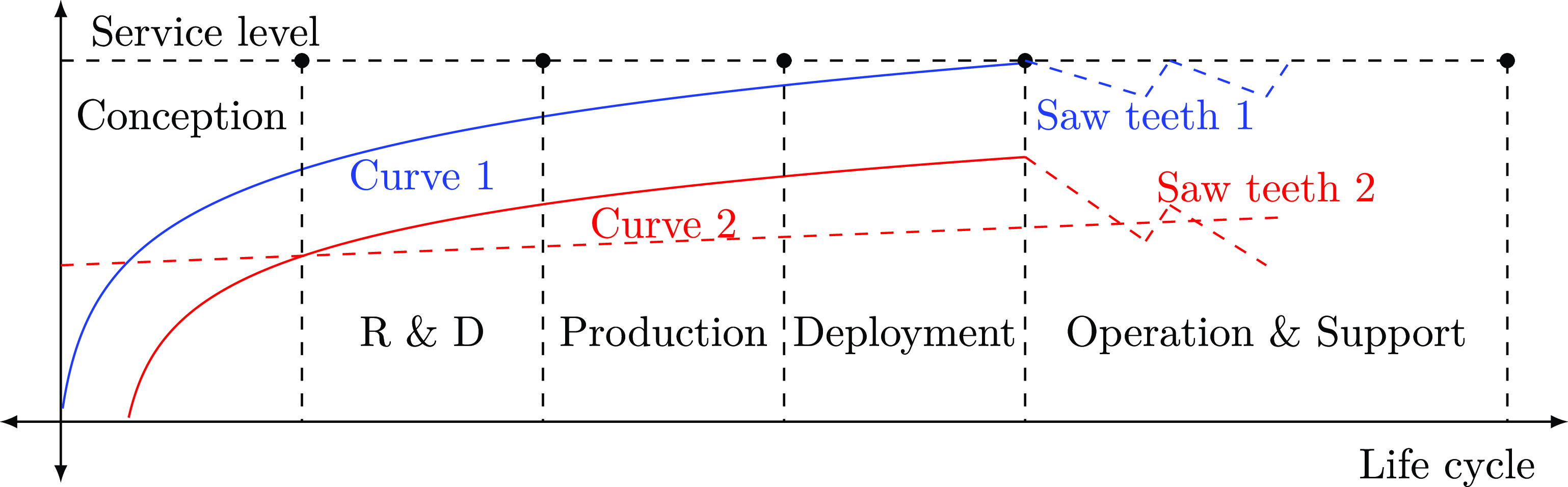
Figure 2 shows the behaviour of support performance for an aircraft fleet. It considers the entire lifecycle from the conceptual phase through conception, research and development, production, operation and support and disposal.

Figure 2.

Observed support performance behaviour.

From the beginning of the conceptual phase to the delivery of the first aircraft, there is an expected growth in service level and dependability requirements (Curve 1). A late entry of supportability requirements can lead to the case of Curve 2.

By observing what happens after the delivery of the first aircraft, the service levels may present degradation that, if not treated properly and in a timely manner, would imply benefit/cost degradation for the fleet. The performance demonstrated in Saw teeth 1 considers system that automatically realigns and corrects the entire maintenance and support programme to prevent such eventual degradation.

A system that adheres to Curve 1 and its continuity throughout the operation and support phase (Saw teeth 1) represents a support system that learns and is resilient throughout the entire fleet lifecycle.

A system that behaves like Curve 2 represents a support and maintenance system that took too long to be developed. It is expected to have a great delay in its maturity target (if it gets there). The performance of this product until its maintenance must therefore imply a series of wastes and extra costs (Saw teeth 2) that the present paper aims to avoid.

We hypothesise that, with the use of the framework proposed, we expect that the system will learn to improve the maintenance plan by intelligently exploring historical data acquired during product development and operation.

3.1 Predictive maintenance for aeronautical engines with machine learning

We accomplished a case study that applies machine learning to aircraft engine sensor data to predict failures. Using historical maintenance logs and sensor readings, we trained models to identify failure patterns and optimise predictive maintenance.

Below is a description of the three common types of machine learning strategies employed.

• • To predict a continuous value we used Random-Forest Regression: time-to-failure (TTF), for each cycle/engine, is the number cycles between that cycle and last cycle of the engine in the training data.

• • To categorise data into one of two distinct cycle bands, we used Binary Classification: if the remaining cycles (TTF) is less than a specific number of cycles (e.g. 30) then the engine will fail in this period. Otherwise the engine is fine.

• • Multi-class Classification was used to categorise failure risk into predefined cycle bands (e.g., 0-15, 16-30, 30+ cycles before failure). These bands allow maintenance teams to prioritise inspections and schedule preventive maintenance before failure occurs.

The insights gained from this case study provide a foundation for applying predictive maintenance models to other aircraft components. Future research will explore integrating these models with the ETTAPS framework to optimise fleet-wide maintenance schedules.

4.1 Maintenance plan development process

Figure 3 presents the flow of information to generate the initial maintenance requirements and appropriately allocate them in the operator’s maintenance plan.

Figure 3.

Process of maintenance plan development using ETTAPS.

The Object Process Methodology (OPM) guided the design of Fig. 3. OPM is a conceptual modeling language and methodology for capturing knowledge and designing systems, specified as ISO/PAS 19,450. OPM was conceived and developed by Dori [Reference Dori38] and is chosen for its ability to concisely represent both the structural (objects) and behavioral (processes) aspects of this complex system.

MSG-3 Data, which gives maintenance guidelines from the Maintenance Steering Group 3 process, is an object in the maintenance plan development process that stands for important information or physical things. Certification data, encompassing data from aircraft type certification, including safety requirements; Dependability Data, representing Reliability, Availability, Maintainability, and Safety (RAMS) data; Maintenance & Operation Profile, detailing the operational context and maintenance history of the aircraft or fleet; Maintenance Requirements, specifying the necessary maintenance tasks and procedures; The Results section contains the outcomes from the Analysing process, such as predictive or prescriptive models.

Maintenance Plan, outlining the scheduled maintenance activities, task allocation and resource allocation; and Field Data, which is collected during the execution of the maintenance activities. The representation of links between objects and processes takes the following form: there are solid arrows that show how objects are used or fed into processes. For example, the MSG-3 Data and Certification Data instrument is used for task compilation, dependability data, the maintenance and operation profile, maintenance requirements and results.

The maintenance plan instruments are used for task allocation and packing. The field data instruments are used for analysis. Control links (dashed arrows) show how objects influence or constrain processes; for example, Dependability Data controls Task Allocation & Packing. Procedural links A depends on B indicate process dependencies; for example, Analysing depends on Field Data.

Some important things to notice about the diagram are the feedback loop: field data informs analysis, and results inform task assignment and packing. This shows that maintenance planning is an iterative process. Multiple objects influence the central task allocation and packing process, which in turn produces the maintenance plan. The diagram emphasises a data-driven approach, highlighting the importance of data from various sources (MSG-3, Certification, Dependability, Field). Finally, it illustrates a systematic process, moving from high-level guidelines to specific tasks and schedules.

4.2 Predicting maintenance needs with machine learning

This system uses historical data to predict future maintenance needs for equipment. Here’s how it works:

• • Learning from the past: We analyse past maintenance data using a technique called supervised learning. This helps us identify a mathematical relationship (the mapping function) between changes in various factors and future maintenance outcomes.

• • Identifying important factors: Not all information in the data is equally important for predicting future needs. We carefully select the most relevant factors (features), such as maintenance date, labour hours and material costs, to improve the accuracy of our predictions.

• • Choosing the best fit: We use a specific technique called random forest regression to explore different types of relationships between the chosen features and the desired outcome. This helps us find the best mathematical formula (the mapping function) to represent that relationship.

• • Making predictions: Once we have a reliable mapping function, we use it to predict future outcomes based on new maintenance data. This allows us to estimate various aspects like:

  1. − Preventive maintenance needs: When might equipment need routine maintenance to avoid failure?

  2. − Failure rates and probabilities: How likely is the equipment to fail in the future?

  3. − Operational availability: How much uptime can we expect from the equipment?

• − Feeding the results: The predictions generated by the mapping function are provided to the IP solver. This solver uses these predictions to optimise future maintenance plans.

ETTAPS employs a two-stage approach. A random forest model (100 trees, max depth 10) predicts component failure probabilities, time-to-failure, remaining useful life and maintenance costs. The probabilities are then used to create a mixed-integer programme (using the Branch & Cut algorithm) that finds the best way to assign and schedule tasks while keeping operational constraints (like task dependencies and resource limits) in mind. Predicted failure probabilities weigh the cost of delaying tasks within the objective function of the optimisation model.

We did not use deep learning (like convolutional neural networks for sensor analysis and recurrent neural networks for time series prediction) yet in this work, nor reinforcement learning (like dynamic scheduling). We are aware that new research on aviation maintenance is exploring these techniques.

ETTAPS uses random forest for prediction and mixed-integer programming for optimisation. Unlike deep learning, ETTAPS effectively handles limited datasets. Unlike reinforcement learning, which often relies on simulations, ETTAPS leverages real-world maintenance data directly.

4.3 Historical records

This work uses a case of an aircraft under development to test the solution proposed. This approach was chosen because of its complexity, which will permit a broad diversity of intricacies that characterise aircraft development.

We chose important components used in aircraft under development that are commercially off-the-shelf components used in many other aircraft on the market. It is also significant that part of the maintenance history records is available: ejection pump; engine; fuel pump; hydraulic pump; starter generator and main battery. Another 80 aircraft repairable components, with some known attribute values, were added to the tests.

The general approach to the estimated parameter values for these 80 items’ attributes was based on making a random choice in the range $\left[ {{x_{min}},{\rm{\;\;}}{x_{max}}} \right]$ according to the engineers’ experience, where $x$ is the parameter average considered.

As to the failure rates, we adopted what was proposed by Smith and Hinchcliffe [Reference Smith and Hinchcliffe39] that defines the observed ranges for a wide number of industry components.

The historical records generated for this work comprised: maintenance date; PM costs; man-hours spent; material consumed; operating hours; and failure probability.

Each time the operations and maintenance schedule block in Fig. 1 sends a record, the learning mechanism is run to generate new slopes and bias. If a certain threshold is surpassed, the IP solver is triggered and a new optimised maintenance plan is generated.

4.4 The TAPP solver

This section presents the mathematical model for the ETTAPS presented in the doctoral thesis of the prime author.

This section provides the rules for any solution method to be adopted, a mathematical description of a system for maintenance planning that accounts for flight and labour times, resource availabilities and due times.

As all variables are expected to be integer and the constraints and objective function are linear, we model TAPP as an Integer Linear Programming formulation.

Let $C = \left\{ {{c_1},{c_2},{c_3},\ldots, {c_{\left| C \right|}}} \right\}$ be a set of aircraft components, being $\left| C \right|$ the size of set $C$ , with the following attributes each:

• • $nam{e_t}$ : a defining name for component ${c_t}$

• • ${\eta _t}$ : the Weibull characteristic life, the time at which 63.2% of the units are likely to fail. More details are available on www.weibull.com

• • ${\beta _t}$ : the Weibull shape parameter, which denotes the degradation rate if it exceeds 1.0

• • $usag{e_t}$ : the usage parameter of component ${c_t}$

A component may have some usage parameters: $FH$ (if the component is controlled by flight hour), $FC$ (by flight cycles), or $MO$ (monthly preventive tasks).

Let $M = \left\{ {General,{\rm{\;\;}}Airframe,{\rm{\;\;}}Powerplant,{\rm{\;\;}}Avionics{\rm{\;\;\;}}Inspection} \right\}$ be a set of aviation mechanics qualifications ( $quali{f_r}$ ) to be properly allocated as needed by the task, and a number of available ( $availabl{e_r}$ ) mechanics for each technical qualification. Each qualification ( $quali{f_r}$ ) has the attribute $wag{e_r}$ expressed in US$/h.

Let $Z = \left\{ {{z_1},{z_2},{z_3},\ldots, {z_{\left| Z \right|}}} \right\}$ be a set of aircraft zones according to the ATA-100 Specification, with the following attributes: $i{d_x}$ (zone ${z_x}$ identifier); $are{a_x}$ (zone area); and $limi{t_x}$ (the maximum number of people to remain simultaneously in the zone ${z_x}$ ). Zones are designated physical areas of an aircraft that identify where maintenance activities occur. A maintenance task can span multiple zones.

Let $P = \left\{ {{p_1},{p_2},{p_3},\ldots, {p_{\left| P \right|}}} \right\}$ be a set of maintenance preparations sub-tasks, that must be performed before or after a maintenance task, to be efficiently allocated with the task to the set of packages, and not duplicated, as multiple tasks may use the same preparations.

Each preparation ${p_k}$ has the following attributes:

• • $nam{e_k}$ : a defining name for preparation ${p_k}$ , e.g., 141BL $ \to $ in zone 141, open door BL

• • $cos{t_k}$ : preparation ${p_k}$ overall cost

• • $m{h_k}$ : estimated preparation ${p_k}$ man-hours

• • $quali{f_k}$ : mechanic qualification needed

• • $qualif_k^r$ : numbers of mechanics for each qualification needed to execute the preparation task ${p_k}$

• • $typ{e_k}$ : a preparation or a follow-on task

• • $nme{c_k}$ : number of mechanics needed

• • $d{t_k}$ : estimated preparation ${p_k}$ downtime

The cost for each preparation task ${p_k}$ is calculated through Equation 1.

(1) \begin{equation} cos{t_k} = m{h_k} \cdot wag{e_{qualif_k^r}} + ma{t_k} + \frac{{m{h_k}}}{{nme{c_k}}} \cdot HOC,{\rm{\;\;}}for{\rm{\;\;}}k \in \left\{ {1,2,3, \ldots, \left| P \right|} \right\}.\end{equation}

Where, $HOC$ is the hourly opportunity cost relative to revenue’s losses, $m{h_k}$ is the number of man-hour required, and $nme{c_k}$ is the quantity of mechanics necessary to accomplish the preparation ${p_k}$ ,.

Let $T = \left\{ {{t_1},{t_2},{t_3},\ldots, {t_{\left| T \right|}}} \right\}$ be a set of maintenance tasks to be efficiently allocated to one of the $S$ packages.

By ‘flight time limit’, we mean the maximum amount of time an aircraft can fly before it requires major maintenance or overhaul. This limit is set based on the Hard Time maintenance strategy, which focuses on scheduled maintenance at specific intervals, rather than relying on monitoring the aircraft’s actual condition.

Each task ${t_j}$ , has the following attributes:

• • $ci{d_j}$ : component identifier

• • $li{m_j}$ : the flight time limits to accomplished task ${t_j}$

• • $pm{c_j}$ : PM cost of ${t_j}$

• • $pmd{t_j}$ : PM downtime of ${t_j}$

• • $pmo{c_j}$ : PM opportunity cost associated to $pmd{t_j}$

• • $cm{c_j}$ : CM cost associated to corrective maintenance of ${t_j}$

• • $cmd{t_j}$ : CM downtime associated to ${t_j}$

• • $cmo{c_j}$ : CM opportunity cost associated to $cmd{t_j}$

• • $ztime_j^{xr}$ : time required for each qualification ${m_r}$ needed for task ${t_j}$ to be executed in zone ${z_x}$

• • $znum_j^{xr}$ : number of mechanics of each qualification ${m_r}$ needed for task ${t_j}$ to be executed in zone ${z_x}$

• • $zon{e_j}$ : aircraft zones where the task will be executed

• • $quali{f_j}$ : mechanic qualification needed

• • $nmec_j^r$ : number of mechanics of qualification ( ${m_r}$ ) needed

• • $prep{s_j}$ : list of preparations necessary to be accomplished prior or after task ${t_j}$

A task ${t_j}$ may be subject to certain constraints if it is included in the same package as another task ${t_q}$ . These constraints establish the relationship between the execution of tasks ${t_j}$ and ${t_q}$ . In this study, we used, $afterStar{t_q}$ which implies only start task ${t_j}$ after a relative task ${t_q}$ finishes and $incompatibl{e_q}$ implying that task ${t_j}$ must not be executed at the same time as task ${t_q}$ .

Constraints of task ${t_j}$ are identified according to the Table 1.

Table 1.

Task relationship codes

An important concept for this chapter is the Opportunity Cost (OC). According to ieser [Reference Wieser40], OC represents the potential benefits an individual, investor or business misses out on when choosing one alternative over another. Depending on the operating hours per day characteristic of an airline, we may establish the hourly opportunity cost ( ${\rm{HOC}}$ ) according to its Revenue per Available Seat Mile (RASM).

While flying, the expenses are relative to fuel consumption and other administrative costs. While in AOG, the expenses are due to maintenance wages and supply. The cost difference: maintenance wages plus supply minus fuel consumption and uptime administrative costs may also be added to the ${\rm{HOC}}$ .

The Equation 2 gives the reliability of a component ${c_t}$ included in task ${t_j}$ planned to stoppage ${s_i}$ occurring at each $sto{p_i}$ interval:

(2) \begin{equation} R_t^i = {e^{ - {{(\frac{{sto{p_i}}}{{{\eta _t}}})}^{{\beta _t}}}}},{\rm{\;\;}}for{\rm{\;\;}}t \in \left\{ {1,2,3, \ldots \left| C \right|} \right\}{\rm{\;\;}},{\rm{\;\;}}for{\rm{\;\;}}i \in \left\{ {1,2,3, \ldots \left| S \right|} \right\}\end{equation}

The Equation 3 gives the reliability of a component ${c_t}$ included in a task ${t_j}$ classified as an Out of Phase task to be executed in ${o_p}$ stoppage at $sto{p_p}$ interval:

(3) \begin{equation} R_t^o = {e^{ - {{(\frac{{sto{p_p}}}{{{\eta _t}}})}^{{\beta _t}}}}},{\rm{\;\;}}for{\rm{\;\;}}t \in \left\{ {1,2,3, \ldots \left| C \right|} \right\}{\rm{\;\;}},{\rm{\;\;}}for{\rm{\;\;}}o \in \left\{ {1,2,3, \ldots \left| O \right|} \right\}\end{equation}

Let ${A_j}$ be a set of $P$ containing the preparations necessary to accomplish the task ${t_j}$ .

Let ${D_{ij}}$ be a set of preparations necessary to accomplish the task ${t_j}$ whenever it is part of a package ${s_i}$ .

\begin{equation*} {D_{ij}} = \left\{ {\begin{array}{l@{\quad}l}{{A_j},} & {}{{\rm{if}}\;{x_{ij}} = 1}\\{0,} & {}{{\rm{if}}\;{x_{ij}} = 0} \end{array}} \right.\end{equation*}

A task may seize preparations if it is included in a package, so its costs and time must be accounted for only once per package ${s_i}$ .

The total number of preparations of a package ${s_i}$ is defined by the set ${B_i}$ , and is calculated as shown in the 4:

(4) \begin{equation} {B_i} = \mathop \bigcup \limits_{j = 1}^m \,{D_{ij}}\end{equation}

The preventive maintenance cost related to labour and material for each task ${t_j}$ allocated in a package is calculated through Equation 5.

(5) \begin{equation} pm{c_j} = \mathop \sum \limits_{r = 1}^{\left| M \right|} mh_j^r \cdot wag{e^r} + ma{t_j},{\rm{\;\;}}for{\rm{\;\;}}t,j \in \left\{ {1,2, \ldots, \left| T \right|} \right\}\end{equation}

The preventive maintenance opportunity cost for each task ${t_j}$ is calculated through Equation 6.

(6) \begin{equation} pmo{c_j} = \mathop \sum \limits_{r = 1}^{\left| M \right|} \frac{{mh_j^r}}{{nmec_j^r}} \cdot HOC,{\rm{\;\;}}for{\rm{\;\;}}t,j \in \left\{ {1,2, \ldots, \left| T \right|} \right\}\end{equation}

Expression $\mathop \sum \nolimits_{r = 1}^{\left| M \right|} \frac{{mh_j^r}}{{nmec_j^r}}$ represents the PM downtime $pmd{t_j}$ .

The total preventive maintenance cost for each task ${t_j}$ is given by Equation 7

(7) \begin{equation} pmt{c_j} = pm{c_j} + pmo{c_j},{\rm{\;\;}}for{\rm{\;\;}}j \in {\rm{\;\;}}\left\{ {1,2, \ldots, \left| T \right|} \right\}\end{equation}

The Equations 8–10 below give the task ${t_j}$ inherent corrective maintenance (CM) cost calculations:

The corrective maintenance labour and material cost for each task ${t_j}$ is calculated through Equation 8.

(8) \begin{equation} cm{c_j} = \mathop \sum \limits_{r = 1}^{\left| M \right|} mh_j^r \cdot CMCF \cdot wag{e^r} + ma{t_j},{\rm{\;\;}}for{\rm{\;\;}}t,j \in \left\{ {1,2,3, \ldots, \left| T \right|} \right\}\end{equation}

The corrective maintenance opportunity cost for each task ${t_j}$ is calculated through Equation 9.

(9) \begin{equation} cmo{c_j} = \mathop \sum \limits_{r = 1}^{||} \frac{{mh_j^r}}{{nmec_j^r}} \cdot CMTF \cdot HOC,{\rm{\;\;}}for{\rm{\;\;}}j \in \left\{ {1,2,3, \ldots, \left| T \right|} \right\}\end{equation}

Where, $CMCF$ is a cost factor for corrective maintenance that corresponds to the high-complexity of corrective maintenance in comparison to the preventive maintenance. $CMTF$ is the corrective maintenance time factor, which represents the increase in downtime caused by unexpected contingencies and unanticipated logistics demands, $HOC$ is the hourly opportunity cost relative to revenue’s losses, and $mh_j^r$ is the number of man-hour of mechanics with qualification $quali{f_r}$ mechanic required, $wag{e^{quali{f_r}}}$ is the man-hour cost of a mechanic with qualification $quali{f_r}$ required for task ${t_j}$ .

The total corrective maintenance cost is given by Equation 10

(10) \begin{equation} cmt{c_j} = cm{c_j} + cmo{c_j}\end{equation}

Let $S = \left\{ {{s_1},{s_2},{s_3},\ldots, {s_{\left| S \right|}}} \right\}$ be a set of maintenance stoppages (or work packages), each with the attribute $sto{p_i}$ , the aircraft maintenance stoppage, and some other parameters to be updated after optimisation:

• • $cos{t_i}$ : overall work package maintenance cost

• • $d{t_i}$ : overall work package maintenance downtime

• • $prep{s_i}$ : the set of unique subtasks associated to the work package

Let $O = \left\{ {{o_1},{o_2},{o_3},\ldots, {o_{\left| O \right|}}} \right\}$ be a set of out-of-phase (OP) stoppages for some tasks that are anti-economical to fit in the preceding regular work package ${s_i}$ . ${o_p}$ stays between ${s_i}$ and ${s_{i + 1}}$ (the next stoppage). It cannot be allocated to ${s_{i + 1}}$ because the component would fly after it’s due FH.

The individual task executed as out-of-phase has the same inherent costs described by the Equation 10.

The calculation of the overall maintenance cost of an out-of-phase stoppage ${o_p}$ is similar to that one used for a standard work package, ${s_i}$ except for the considerations below:

• • Estimation of the anticipated number of failures between two out-of-phase stoppages. ${o_p}$ where the out-of-phase limit $li{m_p}$ is used instead of the package $sto{p_i}$ interval;

• • There is no preparation cost savings, since each out-of-phase stoppage ${o_p}$ has only one task ${t_j}$ ;

• • The computation considers an out-of-phase factor $OPfactor$ , which defines how important it is to the operator to include out-of-phase stoppages in the maintenance plan.

Let ${B^i} = \left\{ {b_1^i,b_2^i,b_3^i,\ldots, b_{\left| {{B^i}} \right|}^i} \right\}$ be a set of maintenance bins which are partitions of maintenance work packages (Fig. 4). I.e., each package is composed of subsets of tasks grouped by bins of concurrent tasks. These bins hold as many tasks as the number of mechanics of each qualification available or the limit of personnel for the task zone, whichever is less. If this number is exceeded, a new Bin must be used to hold other tasks for the same mechanics (or for the same zone) from the previous Bin.

Figure 4.

Work package bins.

As to the Bin downtime ( $dt_b^i$ ), it may be accounted as the longest task and the overall bins downtime may be minimised by minimising the number of bins.

In general, the task constraints defined in the Table 1 that refer to related tasks in the same Bin would be applied; however, only the $startAfte{r_j}$ and $incompatibl{e_j}$ is managed in this work, as the referred task must be in one of the previous bins and tasks that are not compatible must not be in the same bin.

Any resolution method to be used will output an optimal (or close to optimal) solution that expresses the allocations of tasks and their preparation works to regular packages or to out-of-phase stoppages, and tasks in packages to bins.

To permit this, we define three vectors of binary decision variables: (1) ${X_{ij}}$ , to allocate task ${t_j}$ and its preparations $prep{s_j}$ to work package ${s_i}$ ; (2) ${O_{pj}}$ , to allocate task ${t_j}$ its preparations $prep{s_j}$ , not included in the regular work packages, to out-of-phase stoppage ${o_p}$ ; (3) ${W_{jb}}$ to allocate task ${t_j}$ to bin ${b_b}$ .

• • The binary variables ${X_{ij}} = 1$ if task ${t_j}$ is assigned to maintenance package ${s_i}$ , and 0 otherwise.

• • The binary variables ${O_{pj}} = 1$ if the task ${t_j}$ is assigned to an out-of-phase stoppage ${o_p}$ , and 0 otherwise.

• • The binary variables ${W_{jb}} = 1$ if task ${t_j}$ is allocated to the bin ${b_b}$ , and 0 otherwise.

• • Equation 19 states the Objective Function with four parcels:

• • The Equation 11 corresponds to the package preventive maintenance costs parcel, including the amount relative to the costs of the preparations after respective savings

(11) \begin{equation} pmc_j^i = R_t^i \cdot \left[ {pm{c_j} + pmo{c_j} + \mathop \sum \limits_{q = 1}^{n\left( {{B_i}} \right)} prep{c_q}} \right]\end{equation}

• • The Equation 12 corresponds to the expected corrective maintenance costs if the task ${t_j}$ is included in the package, ${s_i}$

(12) \begin{equation} cmc_j^i = \left( {1 - R_t^i} \right) \cdot \left( {cm{c_j} + cmo{c_j}} \right)\end{equation}

• • The Equation 13 corresponds to the out-of-phase stoppage preventive maintenance cost. In this case, there are no savings as regarding the preparations.

(13) \begin{equation} pmc_j^p = R_t^i \cdot \left[ {pm{c_j} + pmo{c_j} + \mathop \sum \limits_{q = 1}^{n\left( {{A_i}} \right)} prep{c_m}} \right]\end{equation}

• • The Equation 14 corresponds to the expected corrective maintenance costs if the task ${t_j}$ is included in the out-of-phase stoppage ${O_p}$

(14) \begin{equation} cmc_j^p = \left( {1 - R_t^i} \right) \cdot \left( {cm{c_j} + cmo{c_j}} \right)\end{equation}

Equations 15 and 16 calculates the flight hour unused. I.e., how much flight hours the aircraft did not fly for being stopped before its flight limit.

(15) \begin{equation} unusedP_i^j = \left\lceil {\frac{{sto{p_i}}}{{li{m_j}}}} \right\rceil - \frac{{sto{p_i}}}{{li{m_j}}},{\rm{\;\;}}for{\rm{\;\;}}j \in \left\{ {1,2,3,\ldots, \left| T \right|} \right\}{\rm{\;\;}}and{\rm{\;\;}}for{\rm{\;\;}}i \in \left\{ {1,2,3,\ldots, \left| S \right|} \right\}\end{equation}

(16) \begin{equation} unusedO_p^j = \left\lceil {\frac{{sto{p_p}}}{{li{m_j}}}} \right\rceil - \frac{{sto{p_p}}}{{li{m_j}}},{\rm{\;\;}}for{\rm{\;\;}}j \in \left\{ {1,2,3,\ldots, \left| T \right|} \right\}{\rm{\;\;}}and{\rm{\;\;}}for{\rm{\;\;}}i \in \left\{ {1,2,3,\ldots, \left| S \right|} \right\}\end{equation}

Equation 19 states the first Objective Function that minimises the maintenance cost of all tasks $\left| T \right|$ and preparation $\left| P \right|$ in the defined horizon $\left| S \right|$ , if tasks and preparations are allocated to work packages. It also attempts to minimise the unused hours costs.

(17) \begin{equation} task\_cos = \mathop \sum \limits_{i = 1}^{|S|} \mathop \sum \limits_{j = 1}^{\left| T \right|} {X_{ij}}{\rm{*}}\left( {cmp_j^i + cmc_j^i + unusedP_i^j \cdot HOC} \right)\end{equation}

(18) \begin{equation} prep\_costs = \mathop \sum \limits_{p = 1}^{\left| O \right|} \mathop \sum \limits_{j = 1}^{\left| T \right|} {O_{pj}}{\rm{*}}\left( {cmp_j^p + cmc_j^p + unusedo_p^j \cdot HOC} \right)\end{equation}

(19) \begin{equation} Min\left\{ {task\_costs + prep\_costs} \right\}\end{equation}

Subject to:

(20) \begin{equation} {\rm{\;\;}}{X_{ij}} \cdot unusedP_i^j \gt = 0,\;\;for{\rm{\;\;}}j \in \left\{ {1,2,3,\ldots, \left| T \right|} \right\}{\rm{\;\;}}and{\rm{\;\;}}for{\rm{\;\;}}i \in \left\{ {1,2,3,\ldots, \left| S \right|} \right\}\end{equation}

(21) \begin{equation} {O_{pj}} \cdot unusedO_p^j \gt = 0,\;\;for{\rm{\;\;}}j \in \left\{ {1,2,3,\ldots, \left| T \right|} \right\}{\rm{\;\;}}and{\rm{\;\;}}for{\rm{\;\;}}o \in \left\{ {1,2,3,\ldots, \left| O \right|} \right\}\end{equation}

Equations 20 and 21 hinder a component from flying beyond its time limit.

(22) \begin{equation} \mathop \sum \limits_{i = 1}^{\left| S \right|} {X_{ij}} + \mathop \sum \limits_{p = 1}^{\left| O \right|} {O_{pj}} \gt = \left\lfloor {{{sto{p_{\left| S \right|}}} \over {li{m_j}}}} \right\rfloor, {\rm{\;\;}}for{\rm{\;\;}}j \in \left\{ {1,2,...,\left| T \right|} \right\}\end{equation}

Equation 22 guarantees that the task ${t_j}$ is executed at least $\left\lfloor {\frac{{sto{p_{\left| S \right|}}}}{{li{m_j}}}} \right\rfloor $ times in planned horizon.

(23) \begin{equation} las{t_t} = las{t_t} \cdot \left( {1 - {X_{aj}}} \right) + sto{p_a} \cdot {X_{aj}},{\rm{\;\;}}for{\rm{\;\;}}t \in \left\{ {1,2,\ldots, \left| C \right|} \right\}\end{equation}

For $i \in \left\{ {1,2,\ldots, \left| S \right|} \right\},{\rm{\;\;}}a \in \left\{ {1,2,\ldots, i - 1} \right\}$ , the last component stoppage is calculated (Equation 23).

(24) \begin{equation} \mathop \sum \limits_{k = 1}^{\left| P \right|} \left| {{B_i}} \right| = {X_{ij}}\end{equation}

For $i \in \left\{ {1,2,\ldots, \left| S \right|} \right\},{\rm{\;\;}}k \in \left\{ {1,2,\ldots, \left| P \right|} \right\}$ , if the task is associated to the work package ( ${X_{ij}} = 1$ ), the preparation ${p_k}$ will be unique (Equation 24); i.e., the same door will not be opened or closed more than once.

(25) \begin{equation} \mathop \sum \limits_{r = 1}^{\left| M \right|} \mathop \sum \limits_{x = 1}^{\left| Z \right|} {X_{ij}} \cdot znum_j^{xr} \gt 0,\;\;for{\rm{\;\;}}j \in \left\{ {1,2,\ldots, \left| T \right|} \right\}\end{equation}

For $x \in \left\{ {1,2,\ldots, \left| Z \right|} \right\}$ and $i \in \left\{ {1,2,\ldots, \left| S \right|} \right\}$ , the number of mechanics of task zones must be greater than zero or the task will not be included (Equation 25).

The TAPP is solved at this point; tasks are associated with work packages, but their sequence and packing are not defined. So, we solve a Bin Packing Problem by minimising the number of bins through packing tasks as efficiently as possible.

(26) \begin{equation} minimize{\rm{\;\;}}\left| {{B^i}} \right|\end{equation}

Equation 26 states the second Objective Function that minimises the number of bins. This minimisation also minimises the overall downtime.

Subject to:

(27) \begin{equation} \mathop \sum \limits_{b = 1}^{\left| {{B^i}} \right|} {W_{jb}} = 1,{\rm{\;\;}}for{\rm{\;\;}}j \in \left\{ {1,2,\ldots, \left| T \right|} \right\}\end{equation}

Each task must be in exactly one Bin, if it is associated to the Bin [Reference Kheder, Trigui and Aifaoui12].

(28) \begin{equation} \mathop \sum \limits_{j = 1}^{\left| T \right|} \mathop \sum \limits_{r = 1}^{\left| M \right|} {W_{jb}} \cdot znum_j^{xr} \lt = limi{t_x}\end{equation}

For each ${\rm{\;\;}}b \in \left\{ {1,2,\ldots, \left| {{B^i}} \right|} \right\}$ and for each $x \in \left\{ {1,2,\ldots, \left| Z \right|} \right\}$ , the number of mechanics cannot exceed the zone limit (Equation 28).

(29) \begin{equation} \mathop \sum \limits_{j = 1}^{\left| T \right|} \mathop \sum \limits_{x = 1}^{\left| Z \right|} {W_{jb}} \cdot znum_j^{xr} \lt = availabl{e_r}\end{equation}

For each $b \in \left\{ {1,2,\ldots, \left| {{B^i}} \right|} \right\}$ and for each ${\rm{\;\;}}r \in \left\{ {1,2,\ldots, \left| M \right|} \right\}$ , the number of mechanics cannot exceed the available for each qualification (Equation 29).

(30) \begin{equation} {W_{t1,b1}} \cdot b1 \lt {W_{t2,b2}} \cdot b2,{\rm{\;\;}}for{\rm{\;\;}}\left( {b1,b2} \right) \in \left\{ {1,2,3,\ldots, \left| {{B^i}} \right|} \right\},{\rm{\;\;}}for{\rm{\;\;}}\left( {t1,t2} \right) \in \left\{ {1,2,3,\ldots, \left| T \right|} \right\}\end{equation}

Equation 30 guarantees that task $t2$ will be put in bin $b2$ , which is posterior to bin $b1$ because task $t2$ must start after $t1$ is finished ( $t1{\rm{\;\;}} = {\rm{\;\;}}StartAfte{r_{t2}}$ ).

(31) \begin{equation} X_{ic}^b = 1 - X_{id}^b\end{equation}

For $c,d \in \left\{ {1,2,\ldots, \left| T \right|} \right\},{\rm{\;\;}}i \in \left\{ {1,2,\ldots, \left| S \right|} \right\},$ and $b \in \left\{ {1,2,\ldots, \left| {{B^i}} \right|} \right\}$ ; and for $c{\rm{\;\;}} \in incompatibl{e_d}$ or $d \in incompatibl{e_c}$ , as $c$ and $d$ are segregated tasks, Equation 31 guarantees that they will not be executed in the same bin.

5.1 Optimisation with branch-and-cut and FFD

Following the work of Almgren et al. [Reference Almgren, Andréasson, Patriksson, Strömberg, Wojciechowski and Önnheim41] who utilised the Branch-and-Cut framework and observed a reduction in Branch-and-Bound nodes and simplex iterations for most problem instances with time-dependent costs, we also adopted this approach to solve the integer programming portion of the Task Allocation and Packing problem. Their work aimed to find optimal opportunistic maintenance schedules that maximise the replacement interval, similar to our goals. The mathematical formulation used in this context can be found in subsection 4.4.

This approach is particularly suited for ETTAPS, as it effectively handles the combinatorial complexity of maintenance task allocation by reducing the solution space through intelligent branching.

To enhance the gains in the availability, we implement the use of the First-Fit Decreasing (FFD) proposed by Johnson [Reference Johnson29].

FFD was selected due to its computational efficiency in solving bin-packing-like problems, as opposed to alternative heuristics like Best-Fit or Next-Fit, which do not prioritise larger tasks for earlier allocation.

We also ran simulations to mimic the process depicted in Fig. 1.

5.2 Simulation results

Tests with different steps were conducted to verify the influence of the value of the step in optimisation of grouping tasks around common preparations.

Figure 5 shows the results of simulations involving 85 maintenance tasks scheduled at intervals ranging in [Reference Gunda, Hackett, Kraus, Downs, Jones, McNalley, Bolen and Walker6, Reference Ackert42–Reference Senturk and Ozkol45] flight hours. We analysed these different intervals to understand the potential advantages and disadvantages of using shorter intervals over three years, with a total flight time of 4,500 hours.

These maintenance intervals were selected through a trial-and-error experimental approach, starting at 10-hour intervals with 1-hour increments. This process aimed to identify potential improvements in overall cost and availability. We observed significant variations in the performance of different intervals, leading us to continue experiments with the selected values, which showed meaningful impacts on optimisation outcomes.

Extensive simulations were performed for each interval to assess the impact. The maximum interval (200 hours) was chosen because some components have shorter lifespans and require more frequent maintenance.

Our experiments revealed that increasing the maintenance interval generally leads to improved cost-effectiveness and equipment availability. However, it’s important to note that 200 hours is the minimum interval considered for the tasks in our sample. This minimum interval is often determined by market demands during the initial development phase of a new product. Therefore, all generated maintenance requirements must adhere to these minimum interval limitations.

Table 2 summarises the results of 20 experiments comparing two maintenance scheduling methods: a simple heuristic method and the ETAPPS + FFD optimisation method. Each experiment considered a fixed maintenance interval of 200 hours and a total annual flight time of 1,500 hours.

Table 2.

200-hour steps tasks distribution

Figure 5.

Step length influence.

The simple heuristic method mimics the existing practice of assigning tasks solely based on engineering expertise. In contrast, the ETAPPS + FFD optimisation method utilises both Branch-and-Cut and FFD algorithms to achieve optimal scheduling. The effectiveness of the proposed optimisation model is evident, consistently demonstrating similar levels of improvement across various experiments involving different task numbers and operational profiles.

We also conducted tests with a sample of tasks that are common in commercial transport aircraft. We used the intervals shown in the MPD as the maximum permitted interval for the systems, structures and zonal tasks. We simulated task allocation in packages using the present technique and compared it to the optimised results supplied by ETTAPS. Table 3 shows the results:

Table 3.

Experiments results: 700 tasks and standard profile

The findings consistently showed that using the ETAPPS resulted in an optimised task distribution. The ETTAPS capitalises on the economic benefits of joining tasks that share the same preparations and access. There is also a gain in cost and availability associated with a lower likelihood of system failure.

The worst-case results expected from this work are an optimised maintenance plan, with tasks being allocated to maintenance packages in the most efficient schedule.

The best-case results are the long-term optimisation of costs and improved resilience of the maintenance system, as new data is constantly included in the learning and optimisation process and the task schedule is fine-tuned at each maintenance cycle.

5.3 Predictive modeling with random forest

The random forest regression included in the Scikit-learn Pedregosa et al. [Reference Pedregosa37] package was used to explore the dataset and select the best fit mapping function. Part of the data is dedicated to training the prediction model.

The main results of tests are presented together with the influence of the learning mechanism after some cycles of tests.

At this time, the historical records have not affected optimisation; ML still forecasts a cost increase, but optimised maintenance plan records will feed the learning mechanism, which will probably result in an overall cost reduction.

We extract features such as the time since last maintenance and sensor readings from historical maintenance logs. The random forest model is retrained monthly using a rolling 24-month data window. Retraining improves predictive accuracy (e.g., AUC increases from 0.77 to 0.85), resulting in 27.4% lower maintenance costs and 1.0% increase in availability in five operations/maintenance cycles, according to Table 4.

Table 4.

Influence of ML on optimisation

Features were selected using recursive feature elimination (RFE) to identify the most influential predictors of maintenance needs. The predictive model used 1,500 maintenance records. Limited data availability constrained the sample size. Five-fold cross-validation achieved an average AUC of 0.85, suggesting sufficient generalisation for this application.

Table 4 depicts the effects of using the learning capability on the optimisation process ( ${A_a}$ is the achieved availability). The resilient planner learned after exploring historical data during the maintenance cycles. This confirms the hypothesis.

These results demonstrate ETTAPS’ advantages in cost and availability compared to a baseline scenario. Due to space limitations, detailed cost distributions and task allocations are not included but are available upon request. ETTAPS achieves cost reductions by intelligently grouping tasks based on dependencies and predicted failure probabilities, minimising redundant preparation efforts and overall maintenance downtime. This is reflected in the lower mean costs and improved availability metrics presented in the tables.

5.4 Limitations

As a limitation, the immediate reaction capacity of the resilient maintenance planner was not considered in this work, as the number of records produced during experimentation was not enough to guarantee an acceptable level of confidence. However, with new operating and maintenance records, we believe that soon lower maintenance costs will be observed.

Future work will explore integrating real-time anomaly detection into ETTAPS, enhancing its ability to dynamically adapt to unexpected component failures.

5.5 Qualitative analysis of results

While a comprehensive quantitative validation with real-world data is a subject for future research, we can offer some qualitative insights based on observed trends and expert knowledge. For instance, the model’s tendency to group related tasks within the same maintenance package aligns with established maintenance practices, which aim to minimise aircraft downtime by coordinating maintenance activities. Furthermore, task prioritisation based on predicted failure probabilities is consistent with expert knowledge in risk management for aircraft maintenance, where components with a higher risk of failure are often given priority. These qualitative observations, while not definitive, provide initial support for the practical applicability of the ETTAPS framework.

5.6 Conclusion

The ETTAPS framework, combining branch-and-cut optimisation with first-fit decreasing task grouping and a random forest predictive model, effectively optimises aircraft maintenance plans, improving cost-effectiveness, resource utilisation, and system availability. While further validation with real-world data is needed, the results demonstrate ETTAPS’ potential for achieving resilient and sustainable aviation maintenance practices.

The framework’s modular design makes it adaptable for integration into existing airline maintenance management systems, facilitating deployment without major infrastructural changes.