


Introduction
Sub-polar and temperate glaciers are more complicated than cold ice sheets for radio echo-sounding (RES) surveys, because they have higher ice temperatures (up to the melting point on so-called “warm” glaciers) and a more inhomogeneous internal structure. In summer, a surface layer of water or soaked firn (slush) is formed on their surface. These water-soaked facies result in higher absorption, attenuation, and scattering of radio waves. In some cases this hampers or makes ineffective the use of radars operating in the ultra-high frequency (UHF) and very high frequency (VHF) range, which have been used successfully for sounding of cold ice sheets in Antarctica, Greenland, and the High Arctic.
Results of radio echo-sounding of Svalbard glaciers with different morphology, types of accumulation, range of zones of ice formation and temperature regime, which were obtained by Soviet expeditions between 1974 and 1984 using radars operating in the VHF and high frequency (HF) range, are illustrated in the following sections. Special attention is paid to the influence of melting on results of sounding, to the problem of sounding of accumulation areas of glaciers, and to the investigation of the nature of internal reflections.
UHF Airborne Radio Echo-Sounding of Svalbard Glaciers
Soaked snow (slush) and water on the surface of glaciers are transparent to radio waves in the UHF range. However, they do attenuate radar signals and also increase their reflection from the upper boundary. Melt water accumulating in the snow-firn facies, in streams, and in crevasses also increases radio-wave scattering. These factors reduce the depth of possible sounding and make the identification of bed returns difficult. Therefore, the cold season, particularly the spring months of April and May, are most favourable for measurements on glaciers which experience intense summer melting. However, because of logistical constraints, we managed to undertake most survey flights over Svalbard in the period June—August.
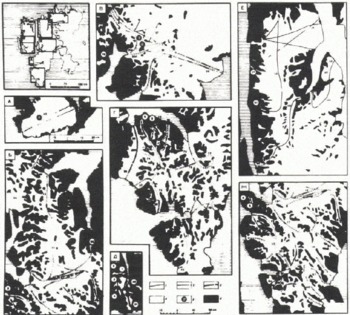
In summer field seasons during 1974–75 and 1978–79 a large number of valley glaciers, ice fields, and ice caps on Spitsbergen and Nordaustlandet (Fig.1) were sounded employing Mikoyan MI-4 and MI-8 helicopters. In 1984, measurements were carried out in some other areas of the archipelago, in particular, on Austfonna in Nordaustlandet (Fig.2), and in the central and southern parts of Spitsbergen. On Spitsbergen, the flights were begun in the middle of May, prior to intense glacier melting.
Index maps showing airborne radio echo-sounding (RES; 440 and 620 MHz) of Svalbard glaciers during the summer field seasons of 1974–75 and 1978–79. Delineation of flight lines of the RES surveys and coding of the types of reflections are shown as follows: 1, from bed; 2, from internal layer; 3, simultaneously from bed and from internal layer; 4, traverses where no reflections from bed and internal layer were registered; 5, location of bore holes; and 6, unglaciated terrain. For glaciers 1–7 data were obtained at a frequency of 440 MHz; for the remainder of the glaciers a frequency of 620 MHz was used. The numbers on the index maps denote glaciers shown in Tables I and II, and on Fig.3.
Index map showing flight lines followed during airborne radio echo-sounding (620 MHz) of glaciers on Nordaustlandet during the summer of 1984, and contours of ice thickness of Austfonna and Vestfonna. Legend: 1, flight lines and flight-line numbers of airborne measurements; 2, field calibration sites on the surface of the ice caps; 3, ice-thickness contours derived from airborne echo-sounding data; and 4, positions of bore holes.

The flights were generally carried out along longitudinal profiles at a flying height of about 300 m above the glacier surface. Navigation along flight lines plotted on 1 : 100 000 and 1 : 500 000 scale maps was carried out by visual sighting to known points. Norsk Polarinstitutt maps based on air-photogrammetric surveys carried out in 1936, 1938, and 1966 were used. In 1984, navigation along flight lines over Nordaustlandet used helicopter navigational equipment to control distances between the initial and final points of the RES profiles.
During the first two field seasons an aircraft-mounted RV-17 radio-altimeter was used. It operated at a frequency of 440 MHz, had a total system performance of 130 dB, and employed a wide-beam antenna of about 100°. The altimeter was successfully used for echo-sounding of small mountain glaciers not more than 150 m in thickness (Reference Kotlyakov, Macheret, Gordiyenko and ZhuravlevMacheret and Zhuravlev 1980). However, for one larger glacier, Fridtjovbreen, internal reflections and bed returns were obtained from ice thicknesses as great as 250 m. In later field seasons, measurements were carried out with an RLS-620 operating at a frequency of 620 MHz. Its total system performance was 185 dB and the radar had a narrow antenna beam width of 18° in E- and H-planes (Reference Kotlyakov, Macheret, Gordiyenko and ZhuravlevKotlyakov and others 1980). Radio echo-sounding measurements were carried out with the RLS-620 over most of the glaciers studied earlier.
Summer radio echo-sounding surveys at the 620 MHz frequency
Analysis of data from radio echo-sounding surveys at the 620 MHz frequency during the summers of 1978—79 are shown in a series of 27 profiles (Fig.3). For several glaciers the interpretations differ from those published earlier by Reference MacheretMacheret (1981) and Reference Macheret and ZhuravlevMacheret and Zhuravlev (1982). The variation is thought to be the result of erroneous interpretation of internal reflections as actual bottom returns (Reference Dowdeswell, Drewry, Liestøl and OrheimDowdeswell and others 1984[a]; Reference Macheret, Vasilenko, Gromyko and ZhuravlevMacheret and others 1984[b]). This revised interpretation is supported by data from airborne RES surveys carried out by British and Norwegian researchers during the spring of 1980 and 1983 with a system which operated at 60 MHz (Reference Dowdeswell, Drewry, Liestøl and OrheimDowdeswell and others 1984[a], Reference Dowdeswell, Drewry, Liestøl and Orheim[b]; Reference DowdeswellDowdeswell unpublished).
Profiles of Svalbard glaciers derived from airborne echo-sounding data acquired during the summer field seasons of 1974—75 and 1978—79 at 440 MHz and 620 MHz, respectively. Legend: 1 and 2, bottom and internal reflecting layer, respectively, according to airborne echo-sounding (RES) data; 3, location of bore holes. For glaciers 1, 3, 4, 5, and 7 RES data were obtained at a frequency of 440 MHz; for the rest of the glaciers at a frequency of 620 MHz. The figures in parentheses correspond to the glacier numbers shown on Fig.1 and in Tables I and II.
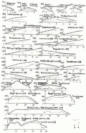
At the 620 MHz frequency, bottom returns throughout most echo-sounding profiles were obtained principally for comparatively small glaciers and ice caps (see Fig.1) not greater than 150–200 m thick and for only a few outlet glaciers not greater than 320–430 m thick. For other relatively large glaciers not greater than 200 m thick, bottom returns were registered with many breaks or gaps in profiles (see Figs 1 and 3) or were not identified at all, especially in accumulation areas and in the heavily crevassed tongues of tide-water glaciers. Examples of such records obtained for Eidembreen and Borebreen are shown in Fig.4a—d. Internal reflections (R), two- and three-fold multiple reflections from glacier surface (S2 and S3), and complicated multiples from the ice surface and the internal boundary (R + S) are also shown.
Examples of 620 MHz frequency records of radar reflections registered at Eidembreen (a and b), Borebreen (c and d), and Doctorbreen (e) in the summer of 1979 (a and c) and spring of 1984 (b, d, and e). T, echo-sounding pulses; S2 and S3, two- and three-fold multiple reflections from the glacier surface; R, reflection from internal layer; B, bottom return; and R + S, multiple reflections from surface and internal boundary.

At Austfonna and Sørfonna in Nordaustlandet, the maximum measured ice thickness was 556 m, and bottom returns were obtained for about 70% of the length of radio echo-sounding profiles. This compares well with 60 MHz RES on Austfonna in 1983 by Reference Dowdeswell, Drewry, Cooper, Gorman, Liestøl and OrheimDowdeswell and others (1986), where bed echoes were recorded over more than 91% of the traverses flown. Three profiles are shown in Fig.5. Bottom returns are generally absent in the heavily crevassed zones on outlet glaciers and in summit parts of the ice caps, where ice thickness exceeds 400—550 m (see Fig.2), On Vestfonna, tracks with bed returns (TBR) are fewer, about 50%. This compares with 52% bed returns observed by Reference Dowdeswell, Drewry, Cooper, Gorman, Liestøl and OrheimDowdeswell and others (1986), Ice thicknesses up to 400 m were recorded in these areas, At Veteranen glacier, returns from as much as 500 m of ice were recorded in 1979 (see Fig.3) and, in 1984, even deeper bottom returns were observed to as much as 625 m.
Thickness of glacier ice on Austfonna-Sørfonna in Nordaustlandet according to RES surveys carried out during the summer of 1984 at a frequency of 620 MHz. Legend: 1, glacier surface; 2 and 3, bottom and internal reflecting layers, respectively, according to analysis of airborne radio echo-sounding data. The location of survey flight lines for the profiles is shown on Fig.2.

Spring radio echo-sounding surveys at the 620 MHz frequency
During aerial RES surveys in May 1984 several glaciers were surveyed (Table I). The same glaciers were surveyed during the summers of 1978 and 1979 at a frequency of 620 MHz (Fig.1) and in the spring of 1980 at 60 MHz (Reference DowdeswellDowdeswell and others 1984[b]). Examples of 620 MHz frequency RES records for Eidembreen, Borebreen, and Doctorbreen are shown in Fig.4.
Track with Bottom Returns (TBR, %) of Selected Spitsbergen Glaciers From Summer and Spring Airborne Radio Echo-Sounding Surveys at Frequencies of 620 MHz (Authors’ Work) and 60 MHz (Reference DowdeswellDowdeswell and Otheks 1984[b])
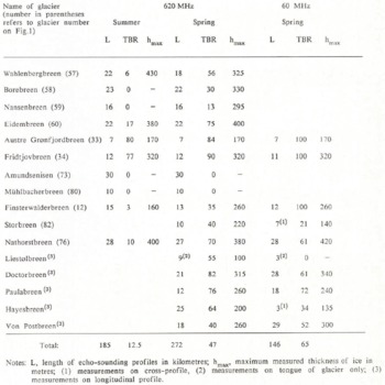
Figs 1, 3, and 4 indicate that on Eidembreen and Borebreen the TBR increased markedly when sounded at 620 MHz in the spring rather than in the summer, from 17 to 75% and from 0 to 30%, respectively. In addition, the pattern of two- and three-fold reflections, as well as of multiple reflections (R + S) have also changed. In particular, the S3 reflections have practically disappeared from the records, and S2 and R + S reflections were observed on only a few plots. Additional information in the form of internal reflections with a complicated form was also present.
The TBR at 620 MHz also increased on other glaciers, many of which were studied repeatedly during the spring of 1984 (Table I). On Amundsenisen and Mühlbacherbreen, bottom returns were not recorded in 1984. Nor were they observed during ground measurements by the RLS-620 radar at Amundsenisen in June 1984, when melting was still insignificant.
Influence of melting on data from high-frequency radio echo-sounding
Our experiments have shown (Reference Kotlyakov, Macheret, Gordiyenko and ZhuravlevMacheret and Zhuravlev 1980) that in accumulation areas of small Spitsbergen glaciers attenuation of radio signals at 440 MHz is 17–34 dB higher during the melt season, and 10 dB higher in the ablation areas. In accumulation areas the amount of additional attenuation depends on many factors: thickness and structure of the ice-firn layer, its temperature regime, intensity of melting and precipitation, depth of soaking, and spatial distribution and thickness of water horizons.
Theoretical assessments of signal attenuation at 440 MHz by a rain-soaked firn layer with a density of 0.5 Mg/m3 and 10–20 m thick gave a range of figures from 8 to 16 dB (Reference DowdeswellDowdeswell and others 1984[b]), and a water layer 5 mm thick spread over the ice surface, about 10 dB (Reference Smith and EvansSmith and Evans 1972). At the 60 MHz frequency these figures are several times less.
According to our calculations when using the 440 MHz altimeter, an additional 20—30 dB attenuation of signal at a flying height of 300 m is equivalent to a reduction in depth of echo-sounding of the glacier bottom which has a bulk ice temperature from 0° to -3°C, by approximately 300350 to 50—150 m when compared to the situation of a dry ice surface and absence of water in the snow—firn layers. At 620 MHz the attenuation may be still greater, and can reach up to 30–40 dB in glacier accumulation areas which have thick snow-firn layers and severe melting. For the RLS-620 radar, this will be equivalent to a decrease in depth of echo-sounding of the bed by approximately 650850 to 250—400 m. As for the 440 MHz equipment during the period of melting, this should result in a significant reduction of TBR on relatively thick glaciers which have tow equilibrium-line altitudes (ELAs). Experimental data on summer and spring measurements at high frequencies support this conclusion (see Figs 1 and 3, and Table I).
The reflection coefficient of the melting glacier surface increases up to values which makes it possible to use the more powerful 620 MHz radar to record n-fold S2 and S3 reflections (see Fig.4a and c). However, in some cases, RES at this frequency may mask bottom returns and reflections from internal layers which makes interpretation of Z-records more difficult. Spring measurements give a different pattern (see Fig.4b, d, and e). This allows us to interpret n-fold reflections as an indicator of surface melting and spatial-temporal changes of snow cover on glaciers. However, this pattern may be complicated by water accumulating in the snow-firn layer at its contact with solid ice. As revealed by the drilling of several shallow bore holes on Austfonna in 1985, these water horizons and lenses may be preserved until the following spring.
Comparison of Airborne Radio Echo-Sounding Data at Frequencies of 620 and 60 MHz
The above data on the thickness of Spitsbergen glaciers obtained from 620 and 60 MHz RES agree rather well, despite differences in flight lines and navigational errors; as a rule, the difference is within 10—15%. Valuable information is also obtained by comparison of data on the TBR of glaciers in the course of spring and summer echo- sounding at various frequencies (Tables I and II).
Track with Bottom Returns (TBR, %) of Selected Spitsbergen and Nordaustlandet Glaciers from Summer and Spring Airborne Radio Echo-Sounding Surveys at Frequencies of 620 MHz (Authors’ Work) and 60 MHz, (Reference DowdeswellDowdeswell and Others 1984[b]; Reference Dowdeswell, Drewry, Cooper, Gorman, Liestøl and OrheimDowdeswell and Others 1986), Respectively

Table I demonstrates that during spring measurements the TBR on the same glaciers at 620 MHz is somewhat lower than data recorded at 60 MHz (51 and 64% respectively), although the total system performance of the 60 MHz Scott Polar Research Institute (SPRI) Mk. IV radar is lower, 144 dB. This is apparently caused by the greater attenuation of radio waves at higher frequencies. The greatest difference was registered at Finsterwalderbreen, 35 and 100%, respectively. But for Doctorbreen, Paulabreen, Nathorstbreen, and Von Postbreen, bottom returns at 620 MHz were measured at a greater distance from the end of the glacier tongue than at 60 MHz, and on Doctorbreen (Fig.6) and Paulabreen they were observed up to the ice divide. On the whole, during spring survey flights in 1984 and 1980 the TBR was about the same: at 620 MHz it was equal to 47%, and at 60 MHz equal to 49% (Reference DowdeswellDowdeswell and others 1984[b]) (length of the profiles of the radio echo-sounding was about 270 and 740 km, respectively).
Data from bore-hole site I in 1975 (A) and from site 2 in 1979 (B-G) on Fridtjovbreen. A: 1, interbeds of dirty ice layers; 2, ice temperature from 1979 measurements; 3, depth of bore hole beyond which the water level in the bore hole, after water addition and withdrawal at the beginning and at the end of drilling periods, attained equilibrium at a permanent depth of 27 m; tm isotherm of ice melting, and 4, glacier bed. B: concentration of ice layers with sub-horizontal orientation of air bubbles. C (density of ice from point measurements): 5, approximation by exponential function (J). D (insoluble mineral admixtures in ice); 6, layers of dirty ice; 7, weight concentration of mineral admixtures in selected layers; E (ice temperature): 8, 1981 measurements; Tm, calculated pressure melting-point of ice; MC, sub-vertical micro-channels 3—5 ?t?ra* found in ice core. F and G (vertical velocity profiles of the glacier according to data from radar logging of bore hole at a frequency of 620 MHz, according to the following calculations): 9, curve τ’(h); 10 and II, curves of layer velocities VL1 and VL2, respectively; 12, graph of velocity calculated on the basis of empirical Equations (1) and (2) (see text). G (curves of the average velocity of radio-wave travel in the glacier υa(h): 13, after two series of measurements; 14, range of υa in each series of measurements; 15 and 10, approximation of curve 13 by twit segments of a straight line; a and c, respectively, depths and errors of definition of the internal reflecting boundary and turning point o£ the curve τ’(h).

But in the summer period at 620 MHz, the TBR of most glaciers was much lower than during spring measurements at 60 MHz. Both the summer and spring measurements at 620 MHz have not recorded bottom returns, mostly in the upper parts of large glaciers and in their lower heavily crevassed parts. The same situation occurred during spring measurements at 60 MHz (Reference Dowdeswell, Drewry, Liestøl and OrheimDowdeswell and Others 1984[a], Reference Dowdeswell, Drewry, Liestøl and Orheim[b]).
Therefore, carrying out the surveys in the spring before melting begins, and reducing the radar frequency from 620 to 60 MHz will not solve the problem of echo- sounding in the accumulation area of many Spitsbergen glaciers (Reference Smith and EvansSmith and Evans 1972; Reference DowdeswellDowdeswell and others 1984[b]). Simple increases in the total system performance of a radar are not able to solve the problem either. The main reason is that, because of melting and refreezing of water, many sub-polar glaciers have higher temperatures of firn and ice in their accumulation areas than ice temperatures in the ablation areas, and some glaciers may have temperatures equal to the pressure melting-point (Reference Troitskiy, Zinger, Koryakin, Markin and MikhaievTroitskiy and others 1975; Reference BaranowskiBaranowski 1977). In addition, the snow-firn layer in many sub-polar glaciers has an inhomogeneous structure because of abundant interbeds and lenses of ice and water inclusions. This results in heavier absorption and attenuation of radio waves of UHF and VHF ranges as well as heavy scattering and masking of bottom returns (Reference Smith and EvansSmith and Evans 1972). This is seen on the records discussed previously (Fig.4). Therefore, heavy scattering may be interpreted to be a qualitative indicator of warmer firn and ice in the accumulation areas of Spitsbergen glaciers (Reference DowdeswellDowdeswell and others 1984[b]). An effective way to reduce scattering is to decrease the radar frequency to 10 MHz or lower (Reference Watts and EnglandWatts and England 1976).
Investigation of the Nature of Internal Reflections
Airborne RES over selected glaciers on Spitsbergen has shown that internal radar reflections (IRR) are present (cf. Reference Macheret, Vasilenko, Gromyko and ZhuravlevMacheret and others 1984[b]; Reference DowdeswellDowdeswell and others 1984[a]). In most cases they could be followed within a depth range from 70 to 200 m, which represents from ¼ of the glacier thickness, and were, for the most part, parallel to the glacier surface. On Z-records they were usually observed as an isolated single-layer echo (Fig.4). An explanation for such IRR may be either: (1) an extended layer with dielectric contrast, or a series of such layers, with a thickness more or less comparable with the transmitted pulse length in the ice (about 30 m for the RLS-620 radar), or (2) a separation of two “semi-infinite” media which differ in their dielectric properties (Reference CloughClough 1977). Extended IRRs within a depth range of 70 to 190 m were also registered by airborne radio echo-sounding at 60 MHz (Reference DowdeswellDowdeswell and others 1984[a], Reference Dowdeswell, Drewry, Liestøl and Orheim[b]). A specific feature of the IRR is that their thickness did not appreciably change with time, within the accuracy of measurements and navigation, and that they were recorded on only relatively thick glaciers (more than 200–250 m thick).
The probable, reason for the extended IRR may be ice layers, differring in density, structure, concentration of mineral inclusions, and chemical impurities from the rest of the ice mass, and water lenses within the glacier (e.g. Millar 1982; Reference Bogorodskiy, Bentley and GudmandsenBogorodskiy and others 1983). These reflections may also be caused by different concentrations of water in cold ice and in ice at the pressure melting-point (Reference Luchininov and MacheretLuchininov and Macheret 1971).
For glaciological interpretations the physical nature of IRR is important; evidence comes from a comparison of radio echo-sounding data with data from deep bore holes (Reference Kotlyakov, Macheret, Gordiyenko and ZhuravlevKotlyakov and others 1980). Such data are available, for example, for Fridtjovbreen, a typical sub-polar glacier (Reference Grigoryan, Bozhinskiy, Krass and MacheretMacheret and others 1985). Studies of Fridtjovbreen included ground and airborne RES, recovery of a deep ice core, and thermal drilling at two sites where IRR were recorded. A description and instrumental investigation of the, ice core was carried out in addition to measurement of the temperature of the ice in bore holes and recording of the water level in one of them. Radar echo-sounding surveys were carried out at frequencies of 440 and 620 MHz along a network of profiles. Along one of the profiles the following frequencies were also used: 450, 686, 735, 786, and 865 MHz.
Two bore holes exceeding 200 m in depth were made; the data collected are shown on Fig.6. In the bore hole at site 1 ice temperatures reached the melting point at a depth of about 80 m (Fig.6a); in the bore hole at site 2 the melting point was reached at about 113 m (Fig.6e). By reference to indirect evidence, the ice temperature at considerable depths is probably close to the pressure melting-point (for example, constant speed of thermal drilling, no sticking of boring tools resulting from icing of the bore hole even if drilling is carried out without antifreeze, absence of sludge, etc.). At depths of less than 115 m the average ice temperature in the bore hole at site 2 equals —1.7° C. The mean integral ice density p within the range of depths less than 119 m is 904 kg m−3 and gradually changes with depth h from 888 to 917 kg m−3 according to the equation:
ρ(h) = 879.5h0 0072.
Volume concentrations of mineral impurities in dirty ice layers generally do not exceed 0.04% (Fig.6d).
A comparison of data from ground and airborne RES obtained during different seasons, at different radar frequencies, and under different flight altitudes has shown that at the ice divide the depth, character, and patterns of the internal reflecting boundary (IRB) are not subject to significant changes over time, taking into account the range of accuracy of measurements and navigational precision. The bore hole at site 1 has a depth of 72 ± 5 m, the one at site 2, 120 ± 10 m. This denotes, first of all, the absence of internal reflecting layers which are “transparent” or “not transparent” for some frequencies; and secondly, that the character of IRB is basically determined by the nature of the IRB and not by equipment parameters or conditions of measurements. Taking this into account, one can, as a first approximation, interpret the IRB at the drilling sites as a comparatively thick homogeneous dielectric layer which is stable with depth.
Measurements of reflected signals from the IRB at bore-hole site 2 provided data of an attenuation of 107 dB at a frequency of 620 MHz. Taking into account the errors of measurements of reflected signals, errors in depth to the IRB, and accuracy of parameters assumed for the calculated model, the reflection coefficient in power from IRB RR = −35 ± 10 dB. At the same time, changes in density, structure, mineral admixtures, and chemical impurities in individual layers or in a series of layers found in the ice core (Fig.6b, c, and d) give, according to our estimates, lower reflection coefficients (from −55 to −100 dB or less), and cannot explain the reported high reflection coefficient from the IRB, The high reflection coefficient from the IRB is, therefore, a result of a dielectrically more contrasting medium, as, for example, from a layer of water-bearing ice or of water.
To investigate the vertical velocity profile of Fridtjovbreen, radar logging of the bore hole at site 2 was carried out (Reference Macheret, Vasilenko, Gromyko and ZhuravlevMacheret and others 1984[a]). Measurements down to a depth of 145 m are given in Fig.6f and g at a specified time:

and Va, the average velocity of radio waves in the glacier:

where τ is the time of travel of a signal from the transmitting antenna on the glacier surface to the receiving antenna in the bore hole, h is the vertical depth of sinking of the receiving antenna (with correction for bending of the bore hole), d is the distance from the transmitting antenna to the bore-hole outlet. The interval of depths corresponding to every linear interval on the diagram, τ ‘(h), is characterized by an approximately constant value of travel time of radio waves and may be interpreted as about homogeneous. In such a layer, the velocity is denoted as layer velocity and is determined as follows:

where Δ hi is the thickness of layer i, Δτi is the time of wave travel in this layer. If a glacier profile consists of two layers with different layer velocities VL1 and VL2, then the average velocity Va2(h) in the lower layer will change in a non-linear way with an increase in thickness of the lower layer h2(Z):

where h1 is the thickness of the upper layer.
On Fig.6, τ’(h), despite rather high dispersion of points resulting mainly from errors of measurements τ, one can see an abrupt change at the depth range of 105–130 m. The curve τ’(h) can be satisfactorily approximated by two linear segments. Therefore, the cross-section of the glacier may be presented as two layers with different layer velocities and, correspondingly, with different dielectric constants. The separation of these layers is at depth h* = 117 ± 12 m. This is very close to the depth of the IRR for the bore hole at site 2 (hR = 120 ± 10 m); therefore, it is suggested that this variation is what produces the IRR, Taking into account small losses in the ice, the following values of layer velocities VL and of dielectric constant ϵ = (c/VL)2 are calculated as follows for the upper layer (0–117 m):
VL1 = 172.2m μs−1, ϵ1 = 3.035; for the lower (117–145 m):
VL2 = 147.7 m μs−1, ϵ2 = 4.125.
Fig.6f and g show VL1 and VL2, and curves
 and
 , produced with an approximation of a Va(h) curve with two linear segments within the same depth interval as the graph τ’(h). They also demonstrate the correlation of average velocity of radio-wave travel in the glacier with depth calculations taking into account the ratio (1) according to the formula of Reference Robin, Evans and BaileyRobin and others (1969)

which describes ∈ of “dry” cold ice as a function of ρ in kg m−3.
From Fig.6f and g, it follows that the value of VL1 differs by no more than 3.3% from
and by only 2% from Vh. This confirms the comparatively high accuracy in the calculations of VL1 and in the validity of the chosen two-layer model of the glacier. The comparatively low mean velocity of radio waves
 , determined through comparison of radio echo-sounding and drilling data for the bore hole at site 1, is explained by a layer of ice at depths h > h* with an average radio-wave velocity close to VL2.
The relationship of the IRR with englacial water is indicated by the following points; depth of the IRR at bore-hole site 1 (hR = 72 ± 5 m) is close to the level where inflow of liquid water from the glacier to the bore hole begins, that is, where englacial water appears (hw = 55—81 m) and the ice temperature reaches the melting point (h0 ≈ 80 m). Also, the level of the water in the bore hole was at 27 m, or 12.6% of the thickness of the glacier. This may be explained by the effects of hydrostatic pressure and the hydraulic connection of the bore hole with the englacial water. The depth of the IRR at bore-hole site 2 (hR = 120 ± 10 m) is close to the level where the ice temperature reaches the melting point (h0 ≈ 113 m). Also, in the ice core there were micro-channels, which are specific to “warm” ice (Reference Zagorodnov and ZotikovZagorodnov and Zotikov 1981) (hw = 100—116 m); the calculated coefficient of reflection from the separation of “cold” and “warm” ice with a low concentration of water (several per cent in volume) is −30 dB (Reference Luchininov and MacheretLuchininov and Macheret 1971) which is very close to the actual measurements (RR = –35 ± 10 dB).
Data on the layer velocity VL allows the content of water in the lower layer to be assessed using the formula of J Paren (Reference Smith and EvansSmith and Evans 1972):

showing the function of the dielectric constant ϵs of water-saturated ice, in which all pores and cavities are filled with water and have a chaotic spatial pattern, in which water content in per cent W = (1 – υ)/100%, where υ = ρd/ρi, ρd and ρi are the density of “dry” glacial ice and of compact ice (ρi = 916.8 kgm−3); ?dand ?w are the dielectric constant of “dry” glacial ice and water (?w = 86). However, Equation (3) provides only the maximum estimate of water in ice. Taking the data of radar logging of the bore hole at site 2 and assuming ϵ1 = 3.035 and ϵs = ϵ2 = 4.125, we get W = 3.8%. The value of may also be estimated according to Equation (2). Taking ρ = 904 kg m−s, we get ϵ = 3.13, and W = 3.4%, The value of ϵ2can also be assessed by the value of the reflection coefficient RR from the IRB, If, starting from the above, we assume that the IRB is a division of two “semi-infinite” media (two-layer model), then:

where

If we assume that RR = –35 ± 10 dB and ϵ1equals 3.035 and 3.13, we get ϵ2 varying from 3.1 to 3.3 and from 3.20 to 3.92, and W changing within 0.23–2.67 and 0.24–2.76%. These estimates are similar to the available data on the water content in warm glaciers of 1–2% (Reference GolubevGolubev 1976).
These data and their analysis suggest that the reason for the IRR at Fridtjovbreen bore-hole sites 1 and 2 is the isothermal layer of “warm” wet ice underlying “dry” cold ice. The depth of the IRR practically coincides with the depth of the isotherm of ice melt in the glacier. Indicators of such a two-layer structure are IRBs, which were recorded along a considerable stretch of this glacier, including cross-profiles. Therefore, it is likely that much of Fridtjovbreen has a two-layer structure.
Relationship of Internal Reflections with the Hydrothermal State and Regime of Glaciers
Similar IRR observed by airborne radio echo-sounding along considerable lengths of many Svalbard glaciers are likely to be of the same nature as those observed at Fridtjovbreen. This allows us to classify as two-layered nearly one-half of the glaciers we studied in Svalbard. However, there is still a chance that in some glaciers, or at least along part of their lengths, IRRs with a similar pattern correspond to reflections from englacial and (or) surface reflectors (for example, water lenses, water streams, cavities, etc.), producing on the RES records a series of hyperbolae encircling their upper parts, or individual branches (Fig.4d and e).
Fig.1 shows that on Spitsbergen the selected glaciers, for which IRR were registered (the supposed indicators of their two-layer structure), occur most often either in the margins of the plateau glaciers or correspond to outlet glaciers. Some of them have (or had in the past) a pattern of warm firn in their accumulation areas and originate in the glacial plateau with warm firn accumulation areas, such as with Fridtjovbreen, the plateau glaciers Amundsenisen and Isachsenfonna, and others. The outlet glaciers descend from plateau glaciers with cold firn in the accumulation areas and negative ice temperature throughout the entire ice thickness such as with Lomonosovfonna (Reference Troitskiy, Zinger, Koryakin, Markin and MikhaievTroitskiy and others 1975; Reference KotlyakovKotlyakov 1985). It was noted previously that the characteristic thickness of ice for these glaciers is greater than 200—250 m, and location of the IRR is usually at to ¼ ½ of their depth. At the same time, in glaciers with a smaller ice thickness, IRR were not usually observed.
The preceding data suggest that glaciers without IRR have cold temperature regimes either throughout the whole ice mass or very nearly to the base of the glacier. This does not, however, preclude the presence of a bottom layer of warm, water-soaked ice, its thickness being beyond the radar resolution in delay time (i.e. about 30 m) as well as the occurrence of water in the bottom layer and on the glacier bed. The IRR should be absent in the accumulation areas of glaciers with warm firn zones, where location of the 0 C isotherm is simitar to the thickness of the active layer, that is, in the range of 10–15 m. Therefore, in some cases, extended IRR may not be recorded on both cold and warm glaciers. In addition, there may be other factors causing the absence of such IRR on records, such as their absence in records which record bottom returns.
The existence on Spitsbergen of glaciers with a bottom layer of ice at the melting temperature was earlier suggested on the basis of observations of ice temperature measured in shallow pits and bore holes (Reference SchyttSchytt 1969; Reference BaranowskiBaranowski 1977). Hypothetical and theoretical ideas were also put forward, that the availability of small amounts of water in the bottom layer of warm ice may result in its outflow from a glacier, thereby producing a notable influence on the mechanical stability of glaciers (Reference KrassKrass 1983).
Analysis of radio echo-sounding data (except for 1984) has demonstrated that of the total number of 43 Spitsbergen glaciers for which IRR were recorded, 16 glaciers have experienced surge behaviour during the past century (Reference LiestølLiestøl 1969; Reference KotlyakovKotlyakov 1985). This accounts for 40% of the total number of selected glaciers under study; data on winter englacial run-off and ice naleds are available for an additional five glaciers, Of the remaining 22 glaciers, 15 are tidal and probably also have englacial run-off during the winter; five are tributary glaciers. In May 1984, for example, we observed differently coloured streams of water discharging into the sea from Eidembreen.
However, surges and naleds were also observed on glaciers which cannot be classified as two-layered ones (for example, Hessbreen, Midre Lovenbreen). On the other hand, ice naleds were found in the tongue of Austre Grønfjordbreen, where hyperbolic IRR were observed from the bottom strata, denoting, apparently, their relation to englacial water accumulations. Hyperbolic reflections were also recorded from the bottom strata of Eidembreen (Fig.4b), where extended IRR were also recorded. In the past 100 years, surges of Spitsbergen glaciers were more often observed from the middle-end of the nineteenth century to the 1920s and 1930s, when the “Little Ice Age” (c. sixteenth to eighteenth centuries) was replaced by warming of the climate, accompanied by glacier recession and thinning. At the same time, many glaciers of the archipelago have apparently experienced changes in the type of accumulation. For some glaciers this could cause cooling of the ice mass from the surface; for other glaciers, warming from the surface (Reference KotlyakovKotlyakov 1985; Reference KotlyakovKotlyakov and Troitskiy 1985). For some glaciers the internal warming is caused by dissipation of energy (Reference KrassKrass 1983; Reference Grigoryan, Bozhinskiy, Krass and MacheretGrigoryan and others 1985), that is, a reconstitution of the glaciers’ thermal regime to form a two-layer one. This mechanism of englacial warming provides a theoretical explanation for the two-layer structure of selected Spitsbergen glaciers, for which extended IRR were registered, and for a good correlation of the calculated depth of location of the ice-melting isotherm in those glaciers which have experimental data on the location of the IRR. In particular, a two-layer structure of Veteranen glacier was theoretically predicted and then supported by radio echo-sounding survey data of 1984.
Conclusions
The RLS-620 radar, which operates at a frequency of 620 MHz, can be successfully employed for radio echo- sounding of a certain type of sub-polar glacier in both the spring and summer. This type of glacier includes comparatively small glaciers up to 200 m thick, as well as some larger ones and ice caps up to 320–625 m thick with, apparently, a colder temperature regime. However, melting considerably worsens the results of radio echo-sounding in the upper parts of many glaciers which are more than 200— 250 m thick. In the accumulation areas of some of these glaciers severe scattering of radio waves caused by englacial inhomogeneities formed by melting and refreezing of water often masks bottom returns even in the case of spring measurements. Studies of Amundsenisen, which has a warm temperature regime and is 700 m thick, have established that this problem may be eliminated by using radar operating in the HF range.
Investigations of the nature of IRR recorded along a considerable length of Fridtjovbreen at a depth range from 70 to 180 m have established that they are caused by a small (of the order of 1–2% in volume) amount of water in the bottom layer and the presence of isothermal ice, which is close to the melting point. Therefore, such IRR may be interpreted as indicators of a special class of two-layered glacier and of the location of the isotherm of melting within them. Many of these glaciers have experienced surge behaviour during the past century and have winter englacial run-off and ice naleds.



