1 Introduction
A ferrofluid is a suspension of magnetizable nano-particles in a carrier fluid. Owing to the ultra-fine particle size and the colloidal stability, a ferrofluid appears as a homogeneous medium, but it displays a variety of novel interfacial phenomena under an external magnetic field (Cowley & Rosensweig Reference Cowley and Rosensweig1967; Miranda Reference Miranda2000; Conroy & Matar Reference Conroy and Matar2015; Feng & Chen Reference Feng and Chen2016). As ferrofluids can be manipulated remotely by a magnetic field, they find applications in mechanical seals, damping systems and loudspeakers (Rosensweig Reference Rosensweig1982; Bailey Reference Bailey1983). More recently, ferrofluids have been studied for potential applications in drug delivery (Voltairas, Fotiadis & Michalis Reference Voltairas, Fotiadis and Michalis2002), treatment of retinal detachment (Mefford et al. Reference Mefford, Woodward, Goff, Vadala, Pierre, Dailey and Riffle2007), control of microfluidic devices (Tan et al. Reference Tan, Nguyen, Yobas and Kang2010) and mechanical measurement in biological tissues (Serwane et al. Reference Serwane, Mongera, Rowghanian, Kealhofer, Lucio, Hockenbery and Campàs2017). In these cases, the dynamics of deformable ferrofluid drops suspended in an immiscible liquid plays an essential role.
The behaviour of a single ferrofluid drop in a static uniform field is well understood. It elongates in the field direction as the magnetic force pulls the drop against interfacial tension. At small deformation, the equilibrium drop shape can be calculated approximately by assuming a prolate spheroidal shape (Bacri & Salin Reference Bacri and Salin1982). At large deformations, numerical computation is necessary (Afkhami et al. Reference Afkhami, Tyler, Renardy, Renardy, Pierre, Woodward and Riffle2010; Rowghanian, Meinhart & Campàs Reference Rowghanian, Meinhart and Campàs2016). Zhu et al. (Reference Zhu, Nguyen, Ramanujan and Huang2011) studied the case of a drop resting on a hydrophobic substrate, with the field direction parallel to the substrate. Other studies have examined the motion of a ferrofluid drop in a magnetic field driven by buoyancy (Korlie et al. Reference Korlie, Mukherjee, Nita, Stevens, Trubatch and Yecko2008) or a field gradient (Afkhami et al. Reference Afkhami, Renardy, Renardy, Riffle and St Pierre2008), drop rupture (Falcucci et al. Reference Falcucci, Chiatti, Succi, Mohamad and Kuzmin2009) and drop relaxation (Rowghanian et al. Reference Rowghanian, Meinhart and Campàs2016).
In a rotating magnetic field, a single ferrofluid drop exhibits an array of interesting dynamics. When the angular velocity of the field – called the driving frequency hereafter – is low, a drop elongates as in a static field and follows the rotation of the field. With increasing driving frequency, the prolate drop may bend (Lācis Reference Lācis1999; Cēbers Reference Cēbers2002) or even break up (Lebedev & Morozov Reference Lebedev and Morozov1997) because of viscous friction in the surrounding medium. At even higher frequencies, the drop may assume several shapes depending on the field strength, ranging from oblate spheroidal at low field strength to a ‘spiny starfish’ shape at high field strength (Bacri, Cēbers & Perzynski Reference Bacri, Cēbers and Perzynski1994; Cēbers & Lācis Reference Cēbers and Lācis1995; Morozov, Engel & Lebedev Reference Morozov, Engel and Lebedev2002; Lebedev et al. Reference Lebedev, Engel, Morozov and Bauke2003). The recent boundary-integral computation of Erdmanis et al. (Reference Erdmanis, Kitenbergs, Perzynski and Cēbers2017) has successfully reproduced many of these shapes.
A pair of ferrofluid drops interact in a static field because of mutually induced magnetization. If their line of centres is initially perpendicular to the external static field, the drops repel while rotating around each other so that their line of centres aligns with the field. Meanwhile, the radial force becomes attractive and the two approach each other and may even coalesce (Chen et al. Reference Chen, Hsueh, Wang and Li2015). A similar scenario occurs in the equivalent problem of two bubbles interacting in a ferrofluid (Lee et al. Reference Lee, Scardovelli, Trubatch and Yecko2010). In both cases, the magnetophoretic interaction can be understood by viewing each drop as an effective magnetic dipole. If an array of ferrofluid drops are constrained in a plane and a static external field is applied perpendicular to the plane, the drops assemble into a hexagonal lattice owing to the magnetic repulsion among them (Chen & Li Reference Chen and Li2010; Timonen et al. Reference Timonen, Latikka, Leibler, Ras and Ikkala2013).
Note that the ferrofluid problem is equivalent to an electrohydrodynamic (EHD) problem for perfect dielectrics, with no free charge and vanished conductivity. Thus, the observations above have counterparts in EHD studies, e.g. on the equilibrium shape of a dielectric drop in an insulating fluid (Garton & Krasucki Reference Garton and Krasucki1964; Sherwood Reference Sherwood1991), the conical ends of a drop under high field strength (Stone, Lister & Brenner Reference Stone, Lister and Brenner1999), and the dielectrophoretic alignment of drops (Baygents, Rivette & Stone Reference Baygents, Rivette and Stone1998).
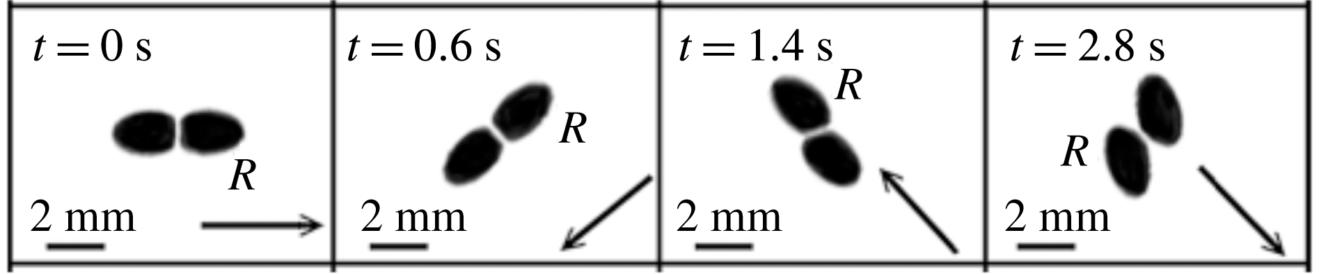
For a pair of ferrofluid drops in a rotating magnetic field, Chen et al. (Reference Chen, Hsueh, Wang and Li2015) observed an intriguing ‘planetary motion’, illustrated in figure 1 and movie 1 in the supplementary material online (available at https://doi.org/10.1017/jfm.2018.261). In their experiments, the millimetre-sized drops elongate in the field direction into an ellipsoidal shape and then spin in phase with the rotating field. The driving frequency is too low for any of the shape instabilities (Lebedev et al. Reference Lebedev, Engel, Morozov and Bauke2003). In addition to the self-spin, the drops revolve around each other in the same sense as the rotation of the field. This planetary revolution does not proceed smoothly with a constant angular velocity, but is punctuated by periodical reversals. The averaged angular velocity is much lower than that of the field. Moreover, a larger number of drops arrange themselves into a regular array that revolves in the sense of the rotating field, at a much lower angular velocity.
Snapshots of the planetary motion of a pair of ferrofluid drops under a magnetic field of uniform strength
 $H_{0}=4488~\text{A}~\text{m}^{-1}$
that rotates anticlockwise at a driving frequency of 1 Hz. The letter
 $R$
marks the drop initially on the right. Reproduced from Chen et al. (Reference Chen, Hsueh, Wang and Li2015) with permission, ©Springer. See also movie 1 in the supplementary material online.

For understanding the cause of the planetary revolution, the most closely related work is perhaps that of Bacri et al. (Reference Bacri, Drame, Kashevsky, Neveu, Perzynski and Redon1995), which concerns a pair of micron-sized highly viscous ferrofluid drops in a rotating field. Because of the small size of the drops, their high viscosity and presumably surface immobilization by surfactant transport, the drops deform little and behave essentially as rigid particles. A pair of solid particles are known to exhibit a revolution around each other (Helgesen, Pieranski & Skjeltorp Reference Helgesen, Pieranski and Skjeltorp1990; Gao et al. Reference Gao, Hulsen, Kang and den Toonder2012) at high enough driving frequency, and the angular velocity of the revolution decreases with the driving frequency. This can be rationalized by treating each particle as a magnetic dipole, and balancing the magnetophoretic forces with a Stokes drag on the particle (Helgesen et al. Reference Helgesen, Pieranski and Skjeltorp1990).
The experiment of Chen et al. (Reference Chen, Hsueh, Wang and Li2015) differs from the solid-particle studies in that the drops are large (radius
 $r_{0}\sim 1$
mm); they deform and are subject to inertial effects. Can their planetary motion be explained by the same dipole model, or does it involve distinct mechanisms? Are there other modes of interaction between deformable ferrofluid drops? These questions have motivated the current study. We have conducted a careful two-dimensional (2-D) numerical simulation of the interaction between a pair of ferrofluid drops in a rotating field. We have reproduced the planetary revolution but found that it arises from different mechanisms. Although the magnetophoretic forces play a role, the most important factor is the hydrodynamic interaction between the elongated drops termed ‘viscous sweeping’. We have also discovered a novel ‘drop-locking’ regime, and confirmed it in new experiments.
2 Governing equations
Consider a pair of ferrofluid drops suspended in an immiscible viscous fluid. Both fluids are assumed to be Newtonian and incompressible, with matched density so gravity or buoyancy is immaterial. The equations of motion are
 $$\begin{eqnarray}\displaystyle & \displaystyle \unicode[STIX]{x1D735}\boldsymbol{\cdot }\boldsymbol{v}=0, & \displaystyle\end{eqnarray}$$
 $$\begin{eqnarray}\displaystyle & \displaystyle \unicode[STIX]{x1D70C}\left(\unicode[STIX]{x2202}_{t}\boldsymbol{v}+\boldsymbol{v}\boldsymbol{\cdot }\unicode[STIX]{x1D735}\boldsymbol{v}\right)=-\unicode[STIX]{x1D735}p+\unicode[STIX]{x1D735}\boldsymbol{\cdot }\left(2\unicode[STIX]{x1D702}\unicode[STIX]{x1D63F}\right)+\unicode[STIX]{x1D735}\boldsymbol{\cdot }\unicode[STIX]{x1D749}_{m}. & \displaystyle\end{eqnarray}$$
Here
 $p$
is the pressure,
 $\boldsymbol{v}$
the velocity,
 $\unicode[STIX]{x1D70C}$
the density and
 $\unicode[STIX]{x1D702}$
the dynamic viscosity.
 $\unicode[STIX]{x1D63F}=(\unicode[STIX]{x1D735}\boldsymbol{v}+\unicode[STIX]{x1D735}\boldsymbol{v}^{\text{T}})/2$
is the rate of deformation tensor. The Maxwell stress tensor
 $\unicode[STIX]{x1D749}_{m}$
represents the magnetic forcing on the ferrofluid. All magnetic equations and quantities in this paper are in SI units. Both fluids are assumed to be dielectric, with instantaneous relaxation of magnetic moments within the ferrofluid (Shliomis & Morozov Reference Shliomis and Morozov1994; Fischer et al.
Reference Fischer, Huke, Lücke and Hempelmann2005; Tackett et al.
Reference Tackett, Thakur, Mosher, Perkins-Harbin, Kumon, Wang, Rablau and Vaishnava2015). Hence,
 $$\begin{eqnarray}\unicode[STIX]{x1D749}_{m}=\unicode[STIX]{x1D707}\boldsymbol{H}\boldsymbol{H}-{\textstyle \frac{1}{2}}\unicode[STIX]{x1D707}H^{2}\boldsymbol{I},\end{eqnarray}$$
where
 $\unicode[STIX]{x1D707}$
is the magnetic permeability of the medium. The surrounding fluid (denoted by subscript
 $s$
) is non-magnetic, so its permeability
 $\unicode[STIX]{x1D707}_{s}$
equals that of vacuum
 $\unicode[STIX]{x1D707}_{0}=4\unicode[STIX]{x03C0}\times 10^{-7}~\text{N}~\text{A}^{-2}$
. For the ferrofluid drop (denoted by subscript
 $d$
),
 $\unicode[STIX]{x1D707}_{d}=\unicode[STIX]{x1D707}_{0}(1+\unicode[STIX]{x1D712})$
with
 $\unicode[STIX]{x1D712}$
being the magnetic (volume) susceptibility.
 $\boldsymbol{H}$
is the magnetic field vector. As commonly done in the literature (Afkhami et al.
Reference Afkhami, Tyler, Renardy, Renardy, Pierre, Woodward and Riffle2010; Erdmanis et al.
Reference Erdmanis, Kitenbergs, Perzynski and Cēbers2017), we assume magnetostatics so
 $\boldsymbol{H}=-\unicode[STIX]{x1D735}\unicode[STIX]{x1D711}$
is irrotational,
 $\unicode[STIX]{x1D711}$
being the magnetic potential, and the Maxwell equations reduce to
 $$\begin{eqnarray}\unicode[STIX]{x1D735}\boldsymbol{\cdot }(\unicode[STIX]{x1D707}\unicode[STIX]{x1D735}\unicode[STIX]{x1D711})=0.\end{eqnarray}$$
The boundary conditions across the interface between the two fluids are standard:
 $$\begin{eqnarray}\unicode[STIX]{x27E6}\boldsymbol{v}\unicode[STIX]{x27E7}=0,\quad \boldsymbol{n}\boldsymbol{\cdot }\unicode[STIX]{x27E6}\unicode[STIX]{x1D70F}_{\unicode[STIX]{x1D702}}+\unicode[STIX]{x1D749}_{m}\unicode[STIX]{x27E7}\boldsymbol{\cdot }\boldsymbol{t}=0,\quad \unicode[STIX]{x27E6}\unicode[STIX]{x1D711}\unicode[STIX]{x27E7}=0,\quad \unicode[STIX]{x27E6}\unicode[STIX]{x1D707}\boldsymbol{H}\unicode[STIX]{x27E7}\boldsymbol{\cdot }\boldsymbol{n}=0,\end{eqnarray}$$
where
 $\unicode[STIX]{x27E6}\cdot \unicode[STIX]{x27E7}$
denotes the interfacial jump of a quantity,
 $\boldsymbol{n}$
and
 $\boldsymbol{t}$
are the unit normal and tangential vectors, respectively, and
 $\unicode[STIX]{x1D70F}_{\unicode[STIX]{x1D702}}=2\unicode[STIX]{x1D702}\unicode[STIX]{x1D63F}$
is the viscous stress tensor. The normal component of the stress has a jump across the interface due to interfacial tension:
 $$\begin{eqnarray}\boldsymbol{n}\boldsymbol{\cdot }\unicode[STIX]{x27E6}\unicode[STIX]{x1D70F}_{\unicode[STIX]{x1D702}}+\unicode[STIX]{x1D749}_{m}\unicode[STIX]{x27E7}\boldsymbol{\cdot }\boldsymbol{n}+\unicode[STIX]{x27E6}p\unicode[STIX]{x27E7}=\unicode[STIX]{x1D70E}\unicode[STIX]{x1D705},\end{eqnarray}$$
where
 $\unicode[STIX]{x1D70E}$
is the constant interfacial tension and
 $\unicode[STIX]{x1D705}$
the curvature.
We use the volume-of-fluid (VOF) formalism to solve the two-phase ferro-hydrodynamics problem numerically. This modifies the governing equations. First, the interfacial tension is accounted for through a body force term that acts only on the interface:
 $$\begin{eqnarray}\unicode[STIX]{x1D70C}(\unicode[STIX]{x2202}_{t}\boldsymbol{v}+\boldsymbol{v}\boldsymbol{\cdot }\unicode[STIX]{x1D735}\boldsymbol{v})=-\unicode[STIX]{x1D735}p+\unicode[STIX]{x1D735}\boldsymbol{\cdot }(2\unicode[STIX]{x1D702}\unicode[STIX]{x1D63F})+\unicode[STIX]{x1D735}\boldsymbol{\cdot }\unicode[STIX]{x1D749}_{m}+\unicode[STIX]{x1D70E}\unicode[STIX]{x1D705}\unicode[STIX]{x1D6FF}_{s}\boldsymbol{n},\end{eqnarray}$$
where
 $\unicode[STIX]{x1D6FF}_{s}$
is the Dirac delta function at the interface. A volume fraction function
 $c(\boldsymbol{x},t)$
is introduced such that
 $c$
takes the value of 1 in the ferrofluid and 0 in the surrounding medium. Thus
 $c$
marks the location of the interface, and evolves according to an advection equation:
 $$\begin{eqnarray}\unicode[STIX]{x2202}_{t}c+\unicode[STIX]{x1D735}\boldsymbol{\cdot }\left(c\boldsymbol{v}\right)=0.\end{eqnarray}$$
We choose the following reference scales: the initial radius of the circular drops
 $r_{0}$
, the matched density of both fluids
 $\unicode[STIX]{x1D70C}$
, the viscosity of the surrounding medium
 $\unicode[STIX]{x1D702}_{s}$
and the magnitude of the uniform external magnetic field
 $H_{0}$
. The reference time scale is chosen to be
 $t_{0}=\sqrt{\unicode[STIX]{x1D70C}r_{0}^{2}/\unicode[STIX]{x1D707}_{0}H_{0}^{2}}$
. It follows that the reference velocity scale is
 $v_{0}=r_{0}/t_{0}$
, and the reference pressure scale is
 $p_{0}=\unicode[STIX]{x1D707}_{0}H_{0}^{2}$
. Denoting all dimensionless variables using the same symbols, the dimensionless Navier–Stokes equation becomes
 $$\begin{eqnarray}(\unicode[STIX]{x2202}_{t}\boldsymbol{v}+\boldsymbol{v}\boldsymbol{\cdot }\unicode[STIX]{x1D735}\boldsymbol{v})=-\unicode[STIX]{x1D735}p+\sqrt{\frac{1}{La_{m}}}\unicode[STIX]{x1D735}\boldsymbol{\cdot }(2\unicode[STIX]{x1D702}\unicode[STIX]{x1D63F})+\unicode[STIX]{x1D735}\boldsymbol{\cdot }\unicode[STIX]{x1D749}_{m}+\frac{1}{Bo_{m}}\unicode[STIX]{x1D705}\unicode[STIX]{x1D6FF}_{s}\boldsymbol{n}.\end{eqnarray}$$
The magnetic Laplace number
 $La_{m}$
,
 $$\begin{eqnarray}La_{m}=\frac{\unicode[STIX]{x1D707}_{0}H_{0}^{2}\unicode[STIX]{x1D70C}r_{0}^{2}}{\unicode[STIX]{x1D702}_{s}^{2}},\end{eqnarray}$$
represents the ratio of the magnetic and inertial forces over the viscous force, and can be interpreted as the square of a Reynolds number. The magnetic Bond number
 $Bo_{m}$
represents the ratio of magnetic force to interfacial tension,
 $$\begin{eqnarray}Bo_{m}=\frac{\unicode[STIX]{x1D707}_{0}H_{0}^{2}r_{0}}{\unicode[STIX]{x1D70E}}.\end{eqnarray}$$
Other dimensionless numbers that govern the problem are as follows: the dimensionless frequency of the driving field,
 $$\begin{eqnarray}f=\frac{1}{T}\sqrt{\frac{\unicode[STIX]{x1D70C}r_{0}^{2}}{\unicode[STIX]{x1D707}_{0}H_{0}^{2}}},\end{eqnarray}$$
with
 $T$
being the period of rotation of the field; the viscosity ratio
 $$\begin{eqnarray}\unicode[STIX]{x1D709}=\frac{\unicode[STIX]{x1D702}_{d}}{\unicode[STIX]{x1D702}_{s}};\end{eqnarray}$$
and the magnetic (volume) susceptibility of the ferrofluid
 $$\begin{eqnarray}\unicode[STIX]{x1D712}=\frac{\unicode[STIX]{x1D707}_{d}}{\unicode[STIX]{x1D707}_{0}}-1.\end{eqnarray}$$
The magnetic field strength in the current study is sufficiently low that we can ignore the rotational viscosity of the ferrofluid (Shliomis Reference Shliomis1972) and assume linear magnetization. Hence
 $\unicode[STIX]{x1D709}$
and
 $\unicode[STIX]{x1D712}$
are both constants. The latter implies that the magnetic force
 $\unicode[STIX]{x1D735}\boldsymbol{\cdot }\unicode[STIX]{x1D749}_{m}=-(H^{2}/2)\unicode[STIX]{x1D735}\unicode[STIX]{x1D707}$
amounts effectively to a surface force acting on the interface only. From this point on, unless stated otherwise, we use dimensionless variables normalized by the reference scales given above.
3 Problem set-up and numerics
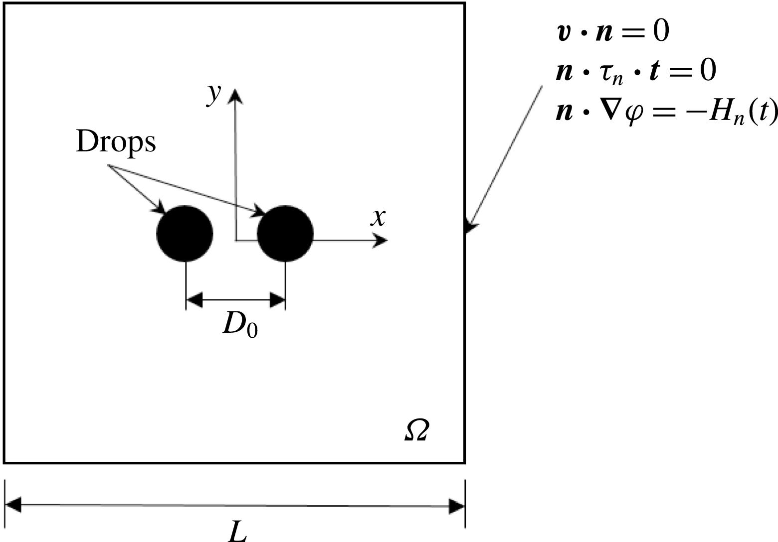
After extensive numerical experimentation, we have realized that a full three-dimensional simulation of two ferrofluid drops in a rotating magnetic field is computationally prohibitive using our current tools. Thus, we will carry out a 2-D simulation using the geometry of figure 2. Two drops of initially circular shape are placed symmetrically in a square domain
 $\unicode[STIX]{x1D6FA}$
, which is large enough that the magnetic field and the velocity field on the boundary
 $\unicode[STIX]{x2202}\unicode[STIX]{x1D6FA}$
are hardly disturbed by the drops. A uniform external field rotates anticlockwise with a constant speed and the dimensionless driving frequency of (2.12). Its orientation is given by the phase angle
 $\unicode[STIX]{x1D703}_{h}=2\unicode[STIX]{x03C0}ft$
with respect to the
 $x$
axis. Thus, we prescribe the rotating magnetic field and impose no penetration of fluid but free slip on
 $\unicode[STIX]{x2202}\unicode[STIX]{x1D6FA}$
:
 $$\begin{eqnarray}\boldsymbol{v}|_{\unicode[STIX]{x2202}\unicode[STIX]{x1D6FA}}\boldsymbol{\cdot }\boldsymbol{n}=0,\quad \boldsymbol{n}\boldsymbol{\cdot }\unicode[STIX]{x1D70F}_{\unicode[STIX]{x1D702}}|_{\unicode[STIX]{x2202}\unicode[STIX]{x1D6FA}}\boldsymbol{\cdot }\boldsymbol{t}=0,\quad \left.\frac{\unicode[STIX]{x2202}\unicode[STIX]{x1D711}}{\unicode[STIX]{x2202}n}\right|_{\unicode[STIX]{x2202}\unicode[STIX]{x1D6FA}}=-H_{n}(t)=-\boldsymbol{n}\boldsymbol{\cdot }(\cos \unicode[STIX]{x1D703}_{h},\sin \unicode[STIX]{x1D703}_{h}).\end{eqnarray}$$
In most of our simulations, the pair of drops start from a horizontal initial orientation.
The 2-D computational domain is a square with the ferrofluid drops initially placed symmetrically inside. On the outer boundary we specify a rotational magnetic field and no-penetration condition with free slip for the velocity.

The VOF computation is carried out using the open-source software package Gerris (Popinet Reference Popinet2003, Reference Popinet2009; López-Herrera, Popinet & Herrada Reference López-Herrera, Popinet and Herrada2011), which uses a second-order accurate fractional-step projection method for time marching, and a finite-volume spatial discretization with a structured quad/octree grid. Both the time step and mesh are adaptive. The discretization of the interfacial tension term
 $\unicode[STIX]{x1D70E}\unicode[STIX]{x1D705}\boldsymbol{n}\unicode[STIX]{x1D6FF}_{s}$
follows the continuous-surface-force (CSF) approach (Brackbill, Kothe & Zemach Reference Brackbill, Kothe and Zemach1992). To interpolate the material properties in the interfacial cells, we use a simple algebraic average for viscosity and a weighted harmonic mean for the magnetic permeability (Afkhami et al.
Reference Afkhami, Tyler, Renardy, Renardy, Pierre, Woodward and Riffle2010):
 $$\begin{eqnarray}\displaystyle & \displaystyle \unicode[STIX]{x1D702}=\frac{c\unicode[STIX]{x1D702}_{d}+(1-c)\unicode[STIX]{x1D702}_{s}}{\unicode[STIX]{x1D702}_{s}}=1+c(\unicode[STIX]{x1D709}-1), & \displaystyle\end{eqnarray}$$
 $$\begin{eqnarray}\displaystyle & \displaystyle \frac{1}{\unicode[STIX]{x1D707}}=\left(\frac{c}{\unicode[STIX]{x1D707}_{d}}+\frac{1-c}{\unicode[STIX]{x1D707}_{0}}\right)\unicode[STIX]{x1D707}_{0}=1+c\left(\frac{1}{1+\unicode[STIX]{x1D712}}-1\right). & \displaystyle\end{eqnarray}$$
We adapt the EHD module in Gerris by setting the electric permittivity
 $\unicode[STIX]{x1D716}$
to the magnetic permeability
 $\unicode[STIX]{x1D707}$
, and the conductivity and free charge density both to zero. Note that in such a VOF formalism, all the boundary conditions across the interface (2.5)–(2.6) are naturally satisfied.
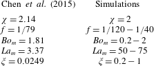
The parameter values are listed in table 1 along with the experimental values in Chen et al. (Reference Chen, Hsueh, Wang and Li2015). We use larger values for the magnetic Laplace number and the viscosity ratio, since the experimental values, corresponding to a low-viscosity ferrofluid and a high-viscosity surrounding liquid, tend to produce strong spurious currents across the interface, which only diminish slowly with mesh refinement. Despite these differences in parameters and the 2-D geometry of the numerical simulations, we have been able to capture the key mechanisms governing the experiment.
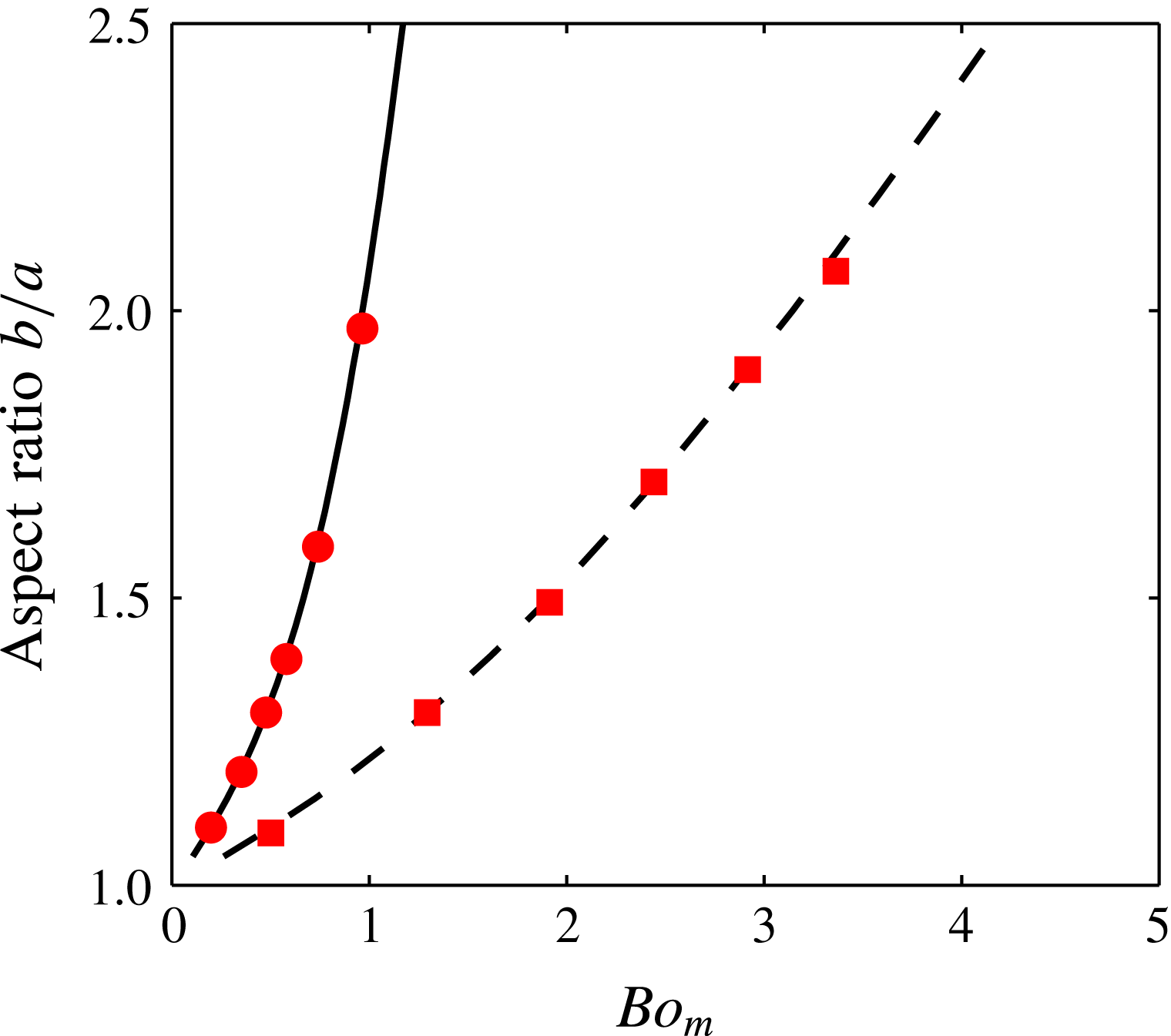
The steady-state drop aspect ratio
 $b/a$
as a function of the magnetic Bond number
 $Bo_{m}$
for two
 $\unicode[STIX]{x1D712}$
values. We compare the numerical results (symbols) with the small-deformation theory (Afkhami et al.
Reference Afkhami, Tyler, Renardy, Renardy, Pierre, Woodward and Riffle2010) for
 $\unicode[STIX]{x1D712}=5$
(solid line) and
 $\unicode[STIX]{x1D712}=2$
(dashed line). The axisymmetric domain is large enough that the magnetic field on the boundary is not disturbed by the drop. The finite-volume cells have sizes ranging from
 $5\times 2^{-9}$
to
 $5\times 2^{-6}$
, with finer cells concentrated on the drop interface.

Comparison of parameters used in the experiment of Chen et al. (Reference Chen, Hsueh, Wang and Li2015) and in our simulations.

We have used two validation tests to assess the performance of the code for simulating two-phase flows with magnetic effects. First, we compute the steady-state shape of a ferrofluid drop in a static uniform field. This test problem is set up in an axisymmetric domain, and we compute the equilibrium aspect ratio of the drop
 $b/a$
as a function of
 $Bo_{m}$
and
 $\unicode[STIX]{x1D712}$
. If the field is weak and the deformation is small, the drop shape can be assumed spheroidal and the problem admits an approximate analytical solution (Afkhami et al.
Reference Afkhami, Tyler, Renardy, Renardy, Pierre, Woodward and Riffle2010). Figure 3 compares the numerical results with the analytical solution for two
 $\unicode[STIX]{x1D712}$
values. Excellent agreement is seen for relatively mild elongation of the drop. At higher
 $Bo_{m}$
or
 $\unicode[STIX]{x1D712}$
values, the drop shape deviates from a perfect spheroid and the discrepancy between the numerical and theoretical results begins to increase.
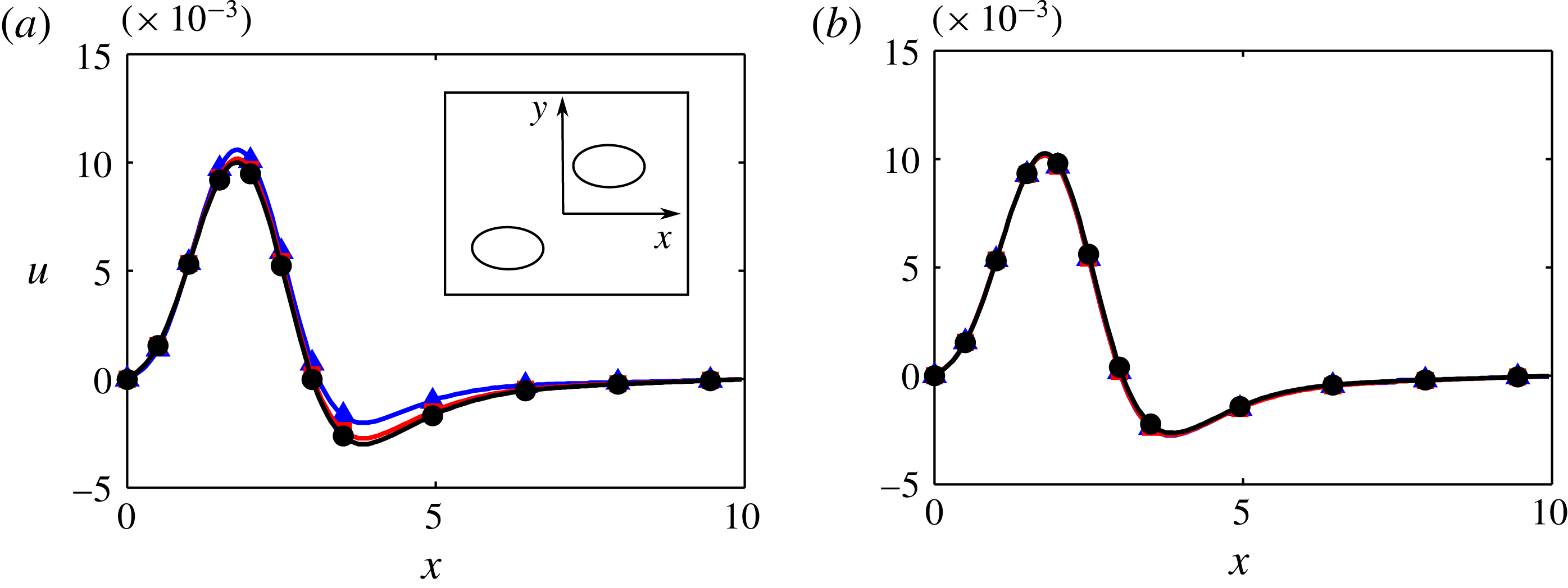
Convergence with mesh refinement (
 $f=1/80$
,
 $Bo_{m}=2$
,
 $\unicode[STIX]{x1D709}=1$
,
 $La_{m}=75$
and
 $D_{0}=4$
). (a)
 $u(x)$
for different finest grid sizes:
 $5\times 2^{-7}$
(▴);
 $5\times 2^{-8}$
(▪);
 $5\times 2^{-9}$
(●). The coarsest grid size is fixed at
 $5\times 2^{-4}$
. (b)
 $u(x)$
for different coarsest grid sizes:
 $5\times 2^{-3}$
(▴);
 $5\times 2^{-4}$
(▪);
 $5\times 2^{-5}$
(●). The finest grid size is fixed at
 $5\times 2^{-8}$
. Temporal discretization is adaptive and the domain length is fixed at
 $L=20$
to save computation time, and the profiles are taken at
 $t=80$
. The inset in (a) shows the shape and position of the drops at this moment.

Further, we demonstrate convergence with respect to grid size and time step refinement and the domain size for the full numerical solution of our drop interaction problem as set up in figure 2. The mesh generator requires specification of the coarsest and finest grid sizes, and we adaptively refine the mesh to deploy the finest grids at the interfaces (Popinet Reference Popinet2009). For a simulation with a representative set of parameters (
 $f=1/80$
,
 $Bo_{m}=2$
,
 $\unicode[STIX]{x1D709}=1$
,
 $La_{m}=75$
and initial separation
 $D_{0}=4$
), figure 4 illustrates mesh convergence using the horizontal velocity profile
 $u(x)$
at
 $t=80$
. The solution converges when the finest mesh size reaches
 $5\times 2^{-8}$
(figure 4
a) and the coarsest mesh size reaches
 $5\times 2^{-4}$
(figure 4
b). Such a grid is used for the rest of the paper except for § 4.3, in which the finest mesh size is reduced to
 $5\times 2^{-9}$
to better resolve the fluid film between the drops. For time stepping, we have found the default adaptive scheme sufficient, with the maximum time step limited by the Courant–Friedrichs–Lewy condition associated with the advection of the fluid and the volume fraction field
 $c$
(Popinet Reference Popinet2003, Reference Popinet2009). For the domain size,
 $L=40$
is large enough for the solution to be independent of
 $L$
.
4 Results and discussion
4.1 Regimes of interaction
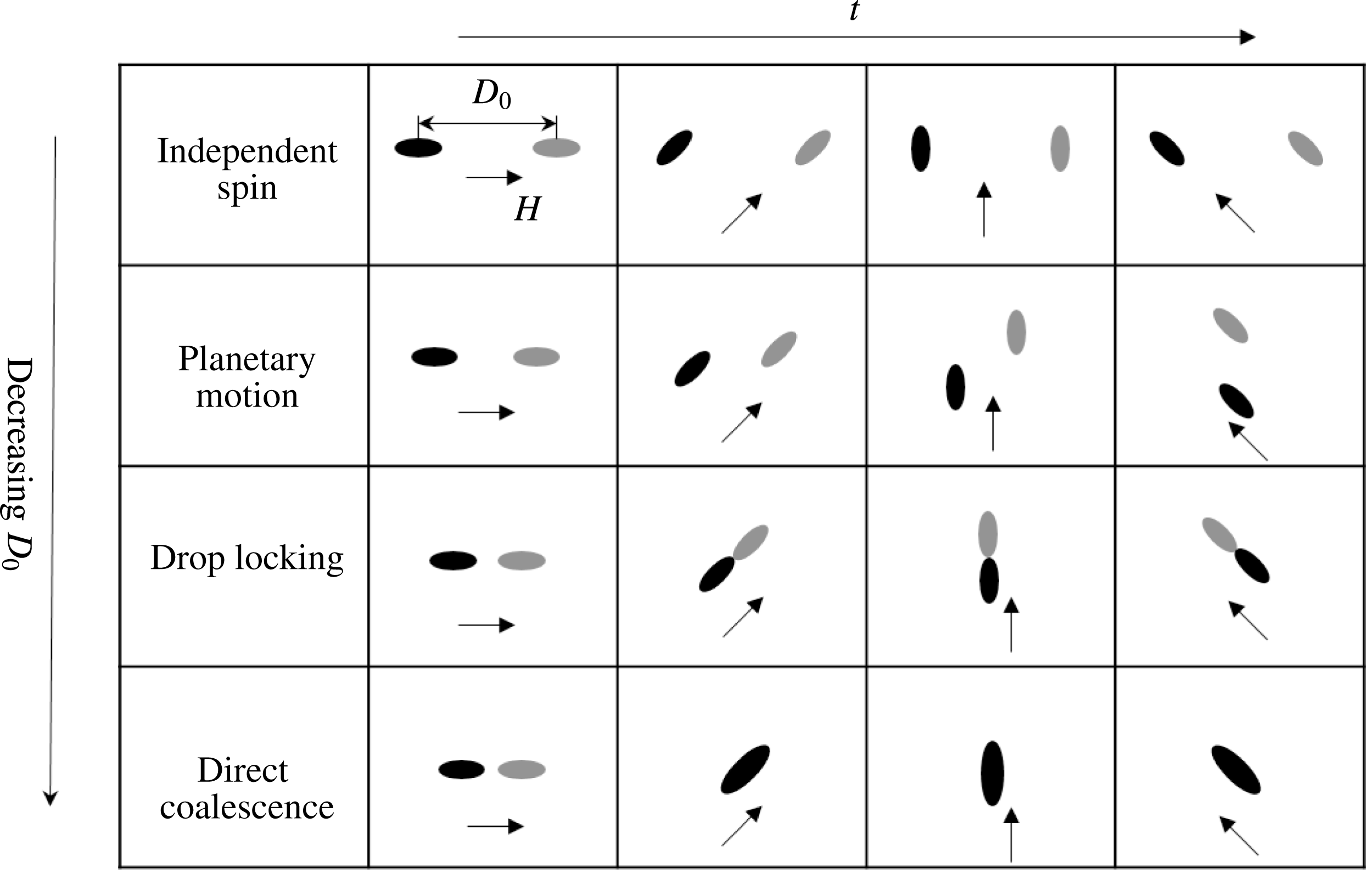
Four regimes of pairwise interaction between the drops have been identified, which can be observed by, for instance, varying the initial separation
 $D_{0}$
of the drops (figure 5).
(i) When
 $D_{0}$
is large, the drops spin individually in phase with the external magnetic field, with negligible interaction.
(ii) At intermediate values of
$D_{0}$
, the drops perform planetary motion; they spin while revolving around each other. The angular velocity of the global revolution is lower than the rotating velocity of the field.(iii) At smaller values of
$D_{0}$
, the pair may attach to each other end-to-end without coalescing, and form a doublet that rotates with the driving frequency. In this ‘drop-locking’ regime, both the phase angle of individual drops and the orientational angle of the pair are locked to the external field, while the drops maintain a small separation between them. This regime may be transient, sometimes preceded by an episode of planetary motion and usually ending in coalescence.(iv) With an even smaller
$D_{0}$
, coalescence takes place right away without going through the locked rotation episode. Afterwards, the merged drop elongates and spins with the field.


Regimes of interaction of the ferrofluid drop pair under an anticlockwise rotating magnetic field.

These regimes agree qualitatively with recent experimental observations (Lu Reference Lu2017). The rest of the paper focuses on the planetary motion and the drop-locking regimes, as well as transitions between different regimes.
4.2 Planetary motion
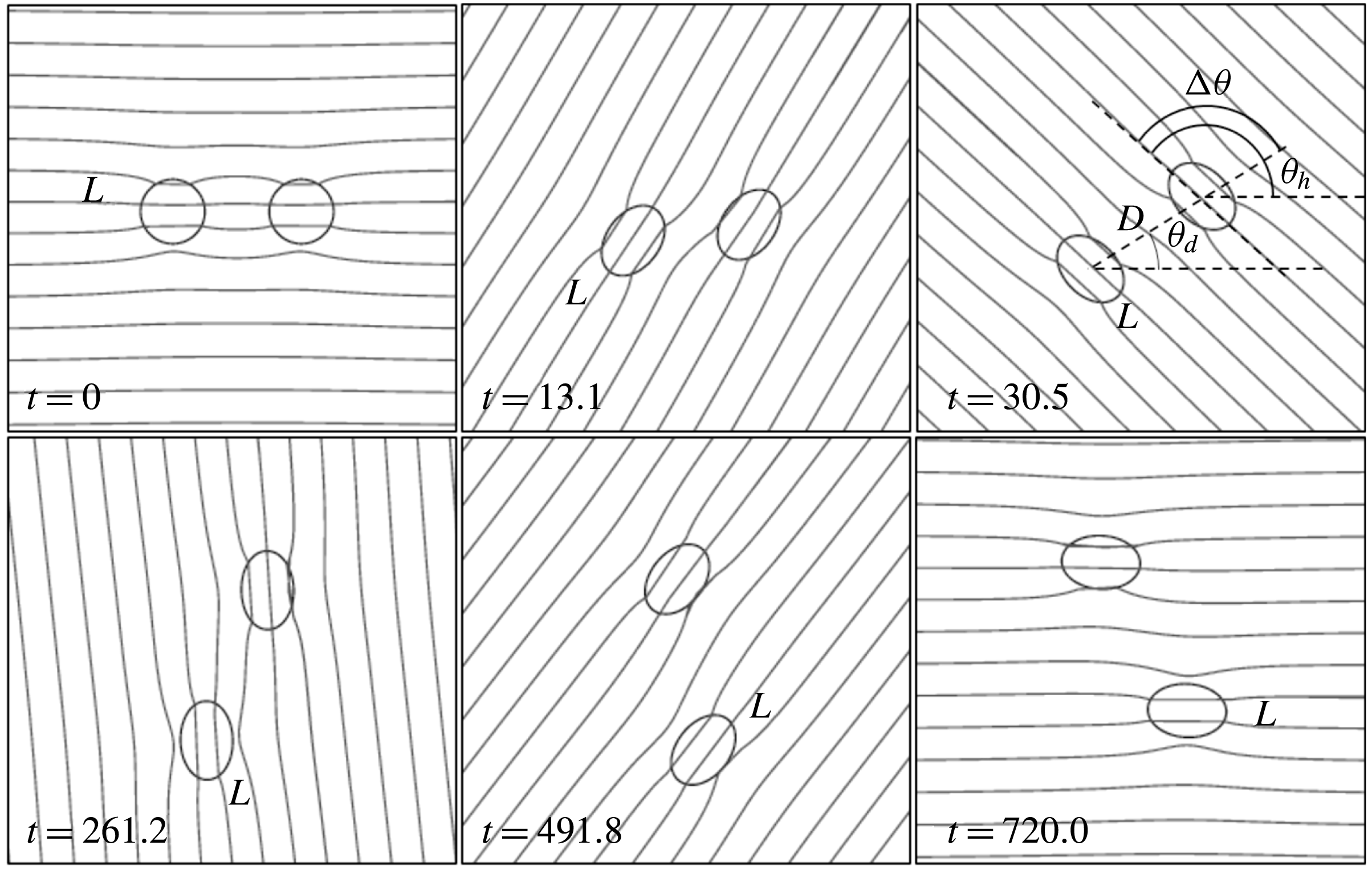
Figure 6 shows a typical simulation of the planetary motion, and an animation (movie 2) can be viewed in the supplementary material online. Each drop spins with the driving frequency of the rotating field
 $f$
, with little phase lag. This is evident from figure 6, where the long axes of the drops align to the field direction within
 $3^{\circ }$
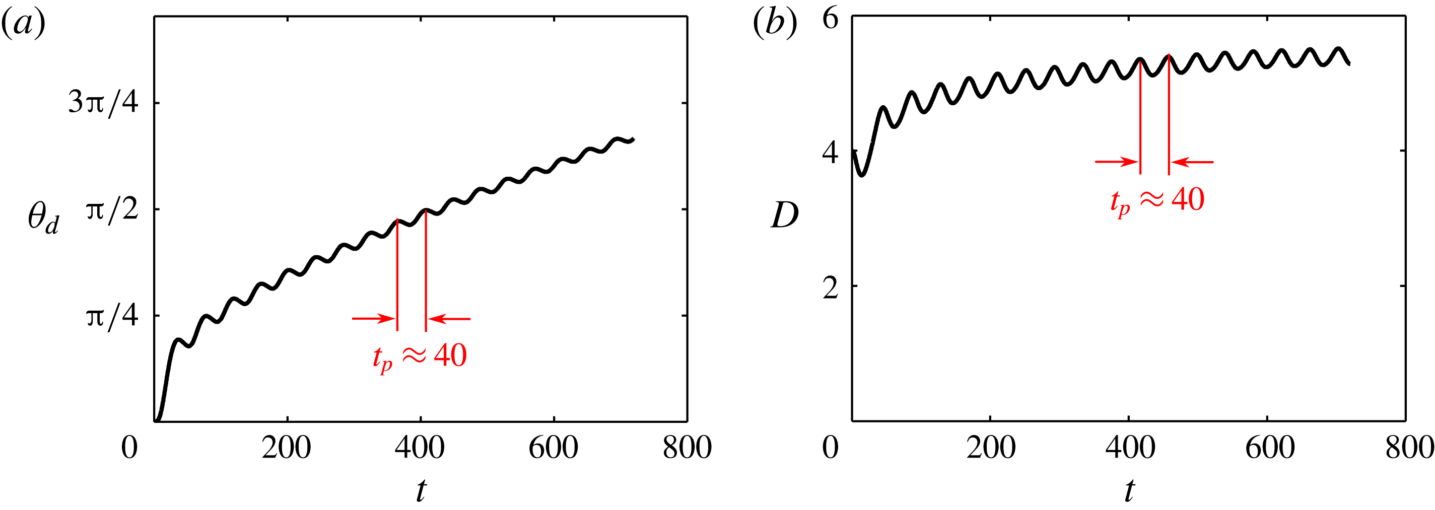
. In the meantime, the drops revolve around each other in the same sense as the rotating field, at a much lower rate. This is demonstrated in figure 7(a) by the increase of the pair orientational angle
 $\unicode[STIX]{x1D703}_{d}(t)$
(see figure 6 for definition). The revolution is not monotonic but suffers periodic small-scale reversals, as has been noted experimentally (Chen et al.
Reference Chen, Hsueh, Wang and Li2015). The drop separation
 $D(t)$
, measured between the centroids of the drops (see figure 6 for definition), shows a similar oscillation, around a mean value that appears to approach a limit in time. These features can be understood from the magnetic and hydrodynamic forces on the drops.
Snapshots of a typical simulation of planetary motion for parameters
 $f=1/80$
,
 $Bo_{m}=2$
,
 $\unicode[STIX]{x1D709}=1$
,
 $La_{m}=75$
and
 $D_{0}=4$
, showing the drops and the magnetic field lines. The letter
 $L$
marks the drop initially on the left. We denote the distance between the centroids of the drops by
 $D$
, and the orientational angle of the pair by
 $\unicode[STIX]{x1D703}_{d}$
. See also movie 2 in the supplementary material online.

(a) The planetary revolution is manifested by the continual increase in the angle
 $\unicode[STIX]{x1D703}_{d}(t)$
. (b) The distance
 $D(t)$
between the centroids of the drops. The parameters are
 $f=1/80$
,
 $Bo_{m}=2$
,
 $\unicode[STIX]{x1D709}=1$
,
 $La_{m}=75$
and
 $D_{0}=4$
. Note the oscillation in both curves with a period
 $t_{p}\approx 1/(2f)=40$
.

4.2.1 Magnetic interaction
The planetary motion resembles the behaviour of two solid magnetic microspheres in a rotating field, which has been accounted for by a dipole model (Helgesen et al. Reference Helgesen, Pieranski and Skjeltorp1990; Bacri et al. Reference Bacri, Drame, Kashevsky, Neveu, Perzynski and Redon1995). Thus, our first enquiry is which of the features observed above can be explained by the simple picture of magnetic dipole–dipole interactions in a viscous medium.
Assuming each drop is a magnetic point dipole, we can derive the following dimensionless 2-D dipolar forces on each drop:
 $$\begin{eqnarray}F_{\unicode[STIX]{x1D703}}=\left(\frac{\unicode[STIX]{x1D712}}{2+\unicode[STIX]{x1D712}}\right)^{2}\frac{\sin (2\unicode[STIX]{x0394}\unicode[STIX]{x1D703})}{D^{3}},\quad F_{r}=-\left(\frac{\unicode[STIX]{x1D712}}{2+\unicode[STIX]{x1D712}}\right)^{2}\frac{\cos (2\unicode[STIX]{x0394}\unicode[STIX]{x1D703})}{D^{3}},\end{eqnarray}$$
in the azimuthal and radial directions, respectively. The forces have been scaled by
 $4\unicode[STIX]{x03C0}\unicode[STIX]{x1D707}_{0}H_{0}^{2}r_{0}$
. The former amounts to a magnetic torque that affects the rotation of the line of the centroids, i.e. the angle
 $\unicode[STIX]{x1D703}_{d}$
. A positive
 $F_{\unicode[STIX]{x1D703}}$
implies an anticlockwise rotation, in the same direction as the rotation of the magnetic field. The latter affects the separation
 $D$
, and a negative
 $F_{r}$
attracts the drops toward each other.
Because the speed of field rotation (
 $\text{d}\unicode[STIX]{x1D703}_{h}/\text{d}t$
) is faster than the rate of planetary revolution (
 $\text{d}\unicode[STIX]{x1D703}_{d}/\text{d}t$
) (figure 7
a), the phase lag
 $\unicode[STIX]{x0394}\unicode[STIX]{x1D703}=\unicode[STIX]{x1D703}_{h}-\unicode[STIX]{x1D703}_{d}$
increases in time. In each round of
 $\unicode[STIX]{x0394}\unicode[STIX]{x1D703}$
,
 $F_{\unicode[STIX]{x1D703}}$
changes sign at
 $\unicode[STIX]{x0394}\unicode[STIX]{x1D703}=0$
,
 $\unicode[STIX]{x03C0}/2$
,
 $\unicode[STIX]{x03C0}$
and
 $3\unicode[STIX]{x03C0}/2$
. Thus, there are four intervals in which the magnetic torque alternately rotates the pair forward (in the same direction as the rotating field) or backward (counter to the field). This explains the small-amplitude oscillations of
 $\unicode[STIX]{x1D703}_{d}$
in figure 7(a). The oscillations in
 $D$
are similarly due to the change in sign of
 $F_{r}$
, although at different
 $\unicode[STIX]{x0394}\unicode[STIX]{x1D703}$
values. Because
 $\text{d}\unicode[STIX]{x1D703}_{h}/\text{d}t$
is much larger than
 $\text{d}\unicode[STIX]{x1D703}_{d}/\text{d}t$
,
 $\unicode[STIX]{x0394}\unicode[STIX]{x1D703}$
increases at almost the same rate as
 $\unicode[STIX]{x1D703}_{h}$
. Hence, the appearance of
 $2\unicode[STIX]{x0394}\unicode[STIX]{x1D703}$
in (4.1) means that
 $\unicode[STIX]{x1D703}_{d}$
and
 $D$
oscillate with a frequency roughly twice the driving frequency
 $f$
(see the period
 $t_{p}$
in figure 7). Furthermore, in an interval of
 $\unicode[STIX]{x0394}\unicode[STIX]{x1D703}$
corresponding to a positive
 $F_{\unicode[STIX]{x1D703}}$
and forward rotation of
 $\unicode[STIX]{x1D703}_{d}$
, the line of centroids chases the driving field so as to slow down the increase of the phase lag
 $\unicode[STIX]{x0394}\unicode[STIX]{x1D703}$
and prolong the time period of forward rotation. Conversely, the time period of backward rotation is shortened. This difference in duration is manifested in figure 7(a). Accumulated over repeated cycles, it produces a forward planetary revolution, in the same sense as the rotating field.
4.2.2 Hydrodynamic interaction
Our ferrofluid drops are not point dipoles, however. For one, they have a finite size and shape, and deform under the influence of the external field
 $\boldsymbol{H}$
. Their motion incurs viscous drag in the surrounding medium. As one elongated drop spins with the driving frequency
 $f$
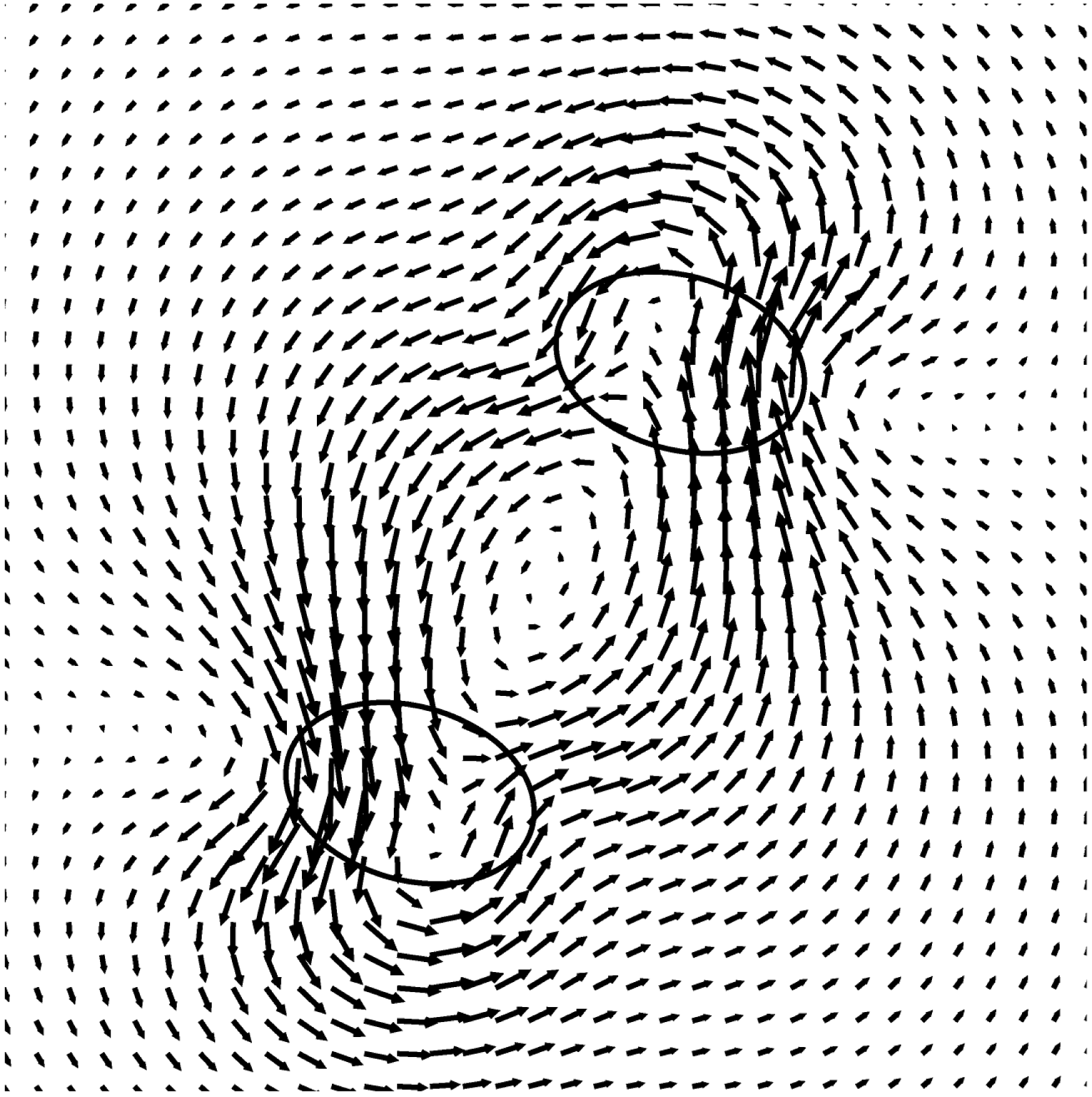
, it creates a flow field that sweeps the other drop forward and induces revolution around each other (figure 8). This ‘viscous sweeping’ effect provides another potential mechanism for the planetary motion, and is key to understanding several novel features of the planetary motion of ferrofluid drops that are absent for point dipoles or solid particles.
Instantaneous velocity field (
 $f=1/80,Bo_{m}=2,\unicode[STIX]{x1D709}=1,La_{m}=75,D_{0}=4$
at
 $t=156.8$
). Only the central region of the domain containing the drops is shown.

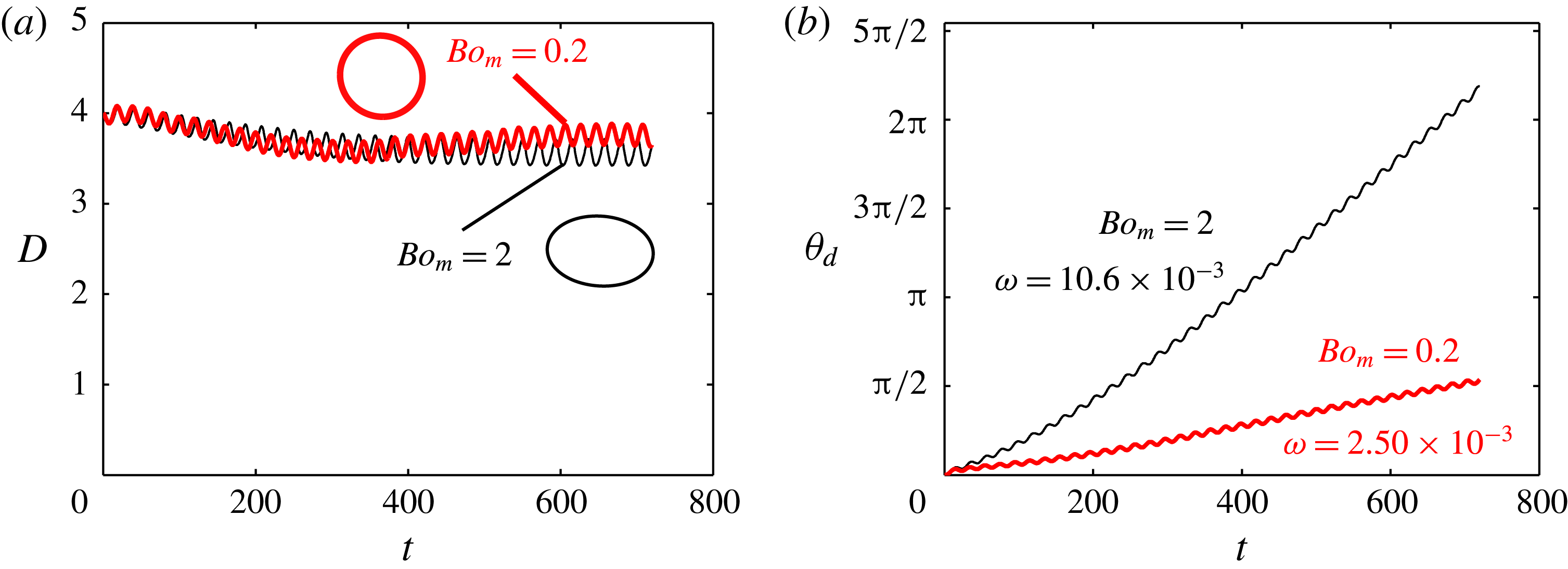
To evaluate the magnitude of the viscous sweeping effect, we vary the drop deformation by reducing the magnetic Bond number
 $Bo_{m}$
from 2 to 0.2. This can be interpreted as increasing the interfacial tension by ten times. In figure 9(a), the ovals represent the typical drop shape at each of the Bond numbers, at the driving frequency
 $f=1/40$
. The drop deformation is indeed greatly reduced, and so will be the viscous sweeping. This change in shape may potentially change the magnetization of the drops and the strength of magnetic interaction. However, figure 9(a) shows little change in the mean value of
 $D$
and its amplitude of the oscillations. Because the radial oscillation is driven by magnetic attraction or repulsion, it follows that there is little change in the magnitude of the magnetic forces. Meanwhile, in figure 9(b), the rate of global revolution has decreased from
 $\unicode[STIX]{x1D714}=10.6\times 10^{-3}$
at
 $Bo_{m}=2$
to
 $\unicode[STIX]{x1D714}=2.50\times 10^{-3}$
at
 $Bo_{m}=0.2$
. Hence, reducing viscous sweeping while keeping the magnetic effect roughly fixed has approximately quartered the rate of planetary revolution. Simulations at other
 $f$
values have confirmed the same trend.
Effect of viscous sweeping probed by varying the magnetic Bond numbers
 $Bo_{m}$
and drop shape:
 $Bo_{m}=2$
(thin line) and
 $Bo_{m}=0.2$
(thick line), with
 $f=1/40$
,
 $\unicode[STIX]{x1D709}=1$
,
 $La_{m}=75$
and
 $D_{0}=4$
. (a) Evolution of the radial distance
 $D$
. The ovals represent the typical drop shapes for the two Bond numbers. (b) Evolution of the pair angle
 $\unicode[STIX]{x1D703}_{d}$
. The angular velocity
 $\unicode[STIX]{x1D714}=d\unicode[STIX]{x1D703}_{d}/dt$
is calculated from the slope of straight lines fitted to the latter part of the
 $\unicode[STIX]{x1D703}_{d}(t)$
curves.

Taking the simplistic view that the dipolar magnetic interaction and viscous sweeping contribute additive parts to the planetary motion, we deduce from the above result that viscous sweeping is a more important mechanism than the magnetophoretic interaction. The same conclusion probably holds in the experiment of Chen et al. (Reference Chen, Hsueh, Wang and Li2015), whose external fluid has higher viscosity than in our numerical study, and thus is more efficient at viscous sweeping. As a side remark, the slower revolution for
 $Bo_{m}=0.2$
means that
 $\unicode[STIX]{x0394}\unicode[STIX]{x1D703}=\unicode[STIX]{x1D703}_{h}-\unicode[STIX]{x1D703}_{d}$
increases slightly faster in time (figure 9
b). This explains the slightly shorter period of oscillation for the rounder drops that is evident in figure 9(a). Its oscillation starts out in phase with that of the elongated drop, but has gained a lead of more than half a period by the end of the simulation.
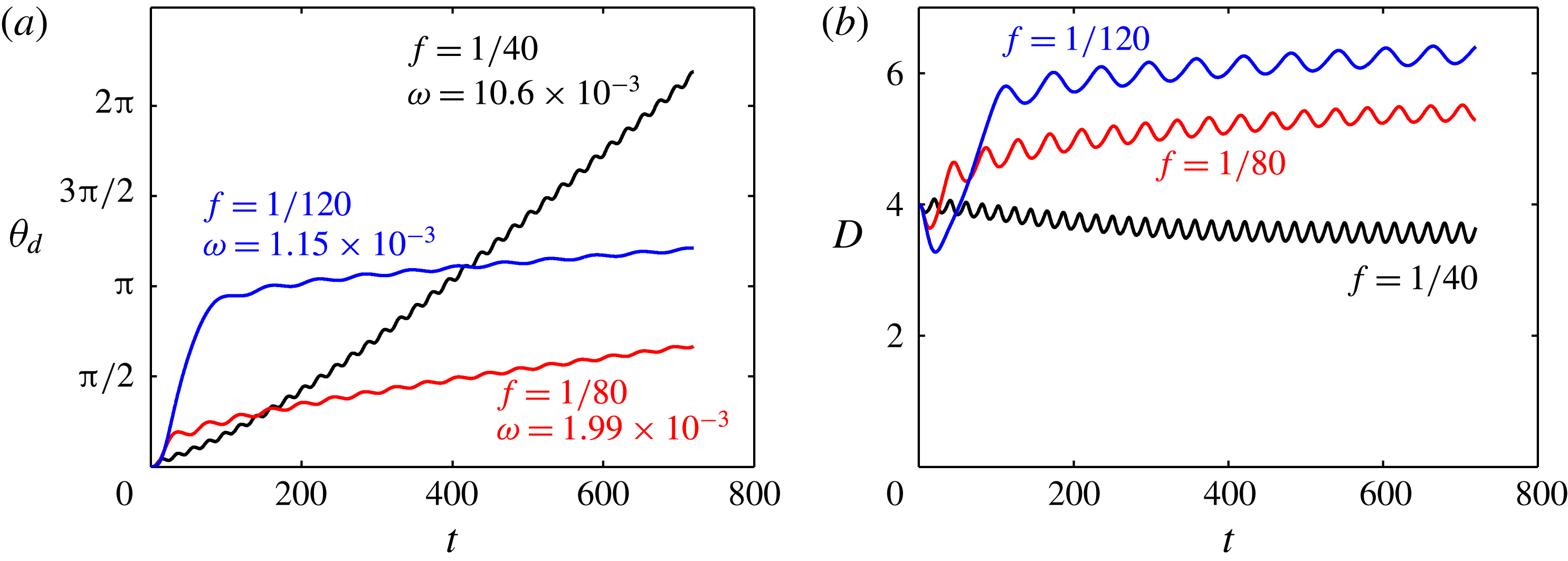
Another novel feature, distinct from its counterpart in solid particles, is how the angular velocity
 $\unicode[STIX]{x1D714}$
of the planetary motion changes with the driving frequency
 $f$
. With all other parameters fixed, increasing
 $f$
causes the pair to revolve around each other at faster
 $\unicode[STIX]{x1D714}$
(figure 10
a). This contrasts the dipole-based solution for solid particles (Helgesen et al.
Reference Helgesen, Pieranski and Skjeltorp1990; Bacri et al.
Reference Bacri, Drame, Kashevsky, Neveu, Perzynski and Redon1995), in which
 $\unicode[STIX]{x1D714}$
decreases with increasing
 $f$
. The latter is because at a faster driving frequency
 $f$
, the planetary revolution of the pair becomes less significant in determining the phase lag
 $\unicode[STIX]{x0394}\unicode[STIX]{x1D703}=\unicode[STIX]{x1D703}_{h}-\unicode[STIX]{x1D703}_{d}$
. As a result, the difference in durations of forward and backward rotation due to
 $\unicode[STIX]{x1D703}_{d}$
also diminishes as the two become closer to cancelling each other. As a cumulative effect, the global revolution
 $\unicode[STIX]{x1D714}$
due to dipolar interaction decreases with increasing
 $f$
. The distinction between ferrofluid drops and solid particles can be rationalized by viscous sweeping, which increases with the spinning velocity
 $f$
of each drop so much that it compensates for any loss in the contribution due to magnetic dipolar interaction to the planetary motion. Note that the drop separation tends to different limits at different frequencies, being closer for higher frequencies (figure 10
b). The reduced separation may also have helped enhance the viscous sweeping.
Effect of the driving frequency
 $f$
on the planetary motion. (a) The evolution of
 $\unicode[STIX]{x1D703}_{d}$
at three frequencies
 $f=1/120$
,
 $1/80$
and
 $1/40$
. The average angular velocity
 $\unicode[STIX]{x1D714}$
is calculated from the slope of straight lines fitted to the latter part of the curves. (b) The evolution of drop separation
 $D$
under the same conditions. The other parameters are fixed:
 $Bo_{m}=2$
,
 $\unicode[STIX]{x1D709}=1$
,
 $La_{m}=75$
and
 $D_{0}=4$
.

4.2.3 Limit separation
We turn to the last novel feature of the ferrodrop planetary motion: the drop separation
 $D$
approaching a limiting mean value independent of the initial separation
 $D_{0}$
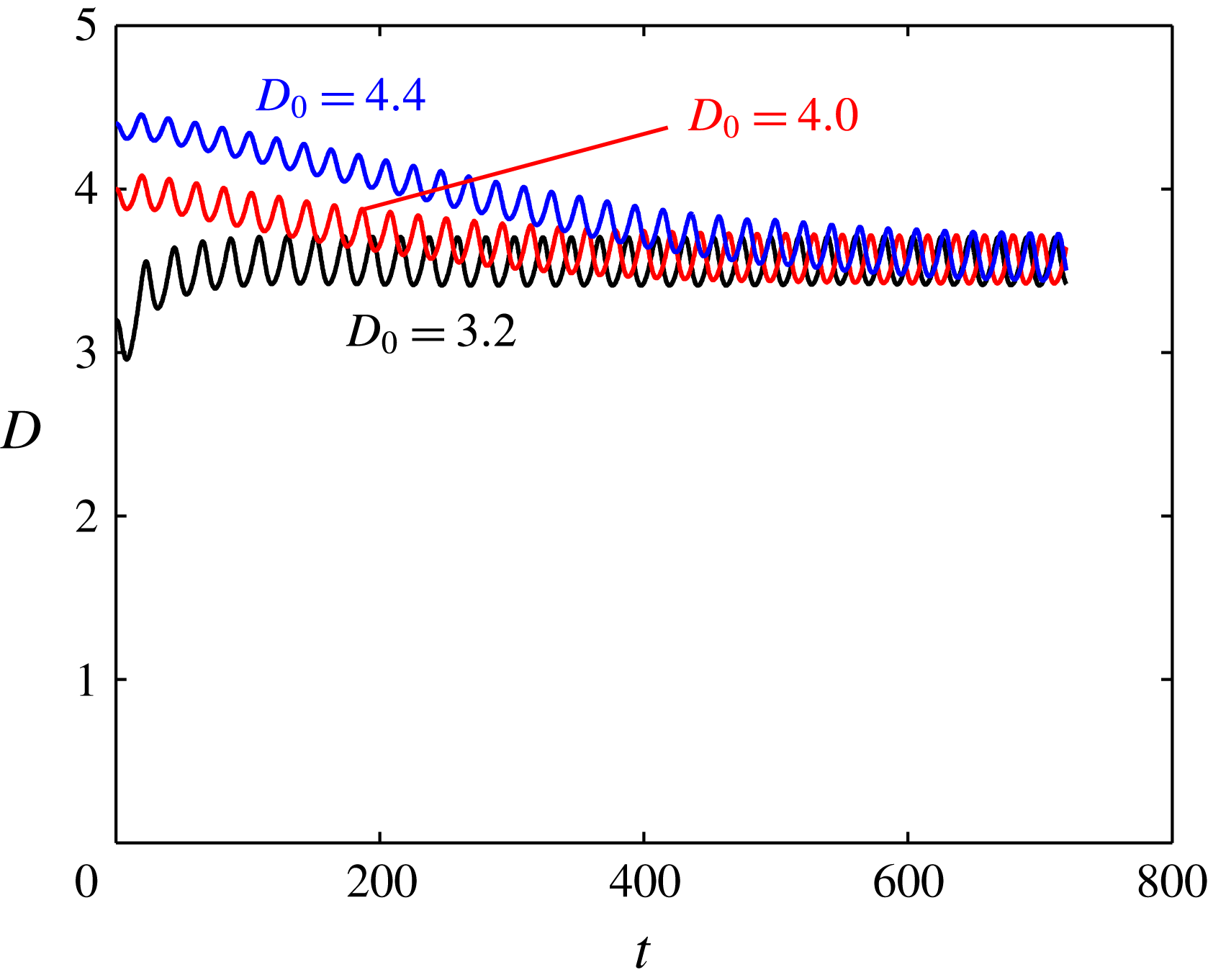
. This has been noted in passing when discussing figures 7 and 10. Figure 11 depicts three trajectories that start from different
 $D_{0}$
toward the same long-time limit mean separation, denoted by
 $D_{s}$
. Initially, the oscillation in the radial distance has smaller amplitudes for the drops starting farther away. This is due to weaker magnetic force at larger distance. As the drops approach the same
 $D_{s}$
, the amplitudes for different cases converge to the same value.
Evolution of the radial distance between the drops starting from different initial separations, for
 $f=1/40,~Bo_{m}=2,~\unicode[STIX]{x1D709}=1$
and
 $La_{m}=75$
.

The limit separation cannot be explained by dipole–dipole interactions. In previous studies of 3-D spheres, the attractive radial magnetic force has greater magnitude and longer duration than the repulsive. Hence, the particles gradually attract and move into contact despite the periodical repulsions (Helgesen et al.
Reference Helgesen, Pieranski and Skjeltorp1990). In two dimensions, the radial magnetic force
 $F_{r}\propto \cos (2\unicode[STIX]{x0394}\unicode[STIX]{x1D703})$
(4.1) is symmetric between the attractive and repulsive phases. Thus, the two cancel over each cycle and do not produce a cumulative drift in
 $D$
. Two solid particles would thus revolve in orbits that retain the initial mean separation
 $D_{0}$
.
Here we examine three hydrodynamic mechanisms that have potentially contributed to the limit separation. The first is inertia. As the magnetic radial force
 $F_{r}$
drives the drops apart or toward each other, the drops will not stop instantaneously when
 $F_{r}$
switches between positive and negative values. Rather, inertia carries them further, overshooting the zeros of
 $F_{r}$
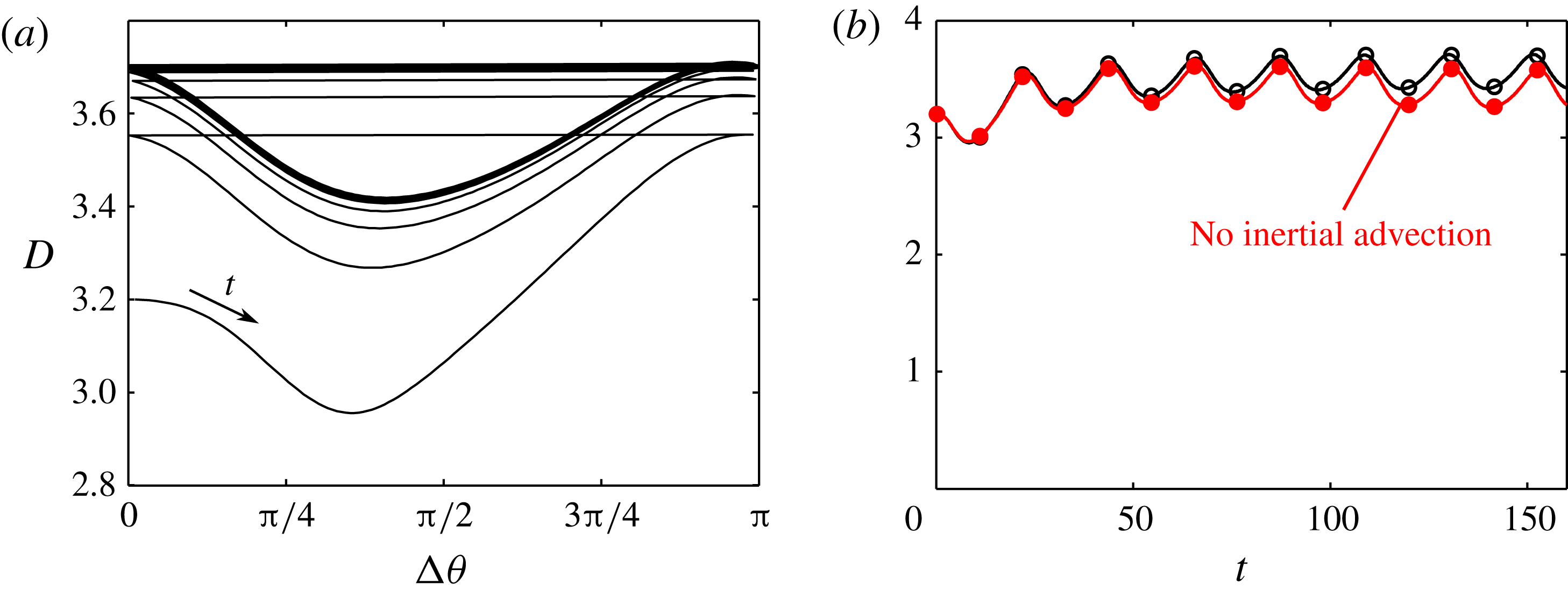
. Figure 12(a) illustrates the overshoot in the
 $D$
-
 $\unicode[STIX]{x0394}\unicode[STIX]{x1D703}$
phase plane by a representative trajectory, the
 $D_{0}=3.2$
case in figure 11.
 $F_{r}$
changes from attraction to repulsion at
 $\unicode[STIX]{x0394}\unicode[STIX]{x1D703}=\unicode[STIX]{x03C0}/4$
. But
 $D$
continues to shrink and reaches its minimum some time after
 $F_{r}$
has turned repulsive. At such a small
 $D$
,
 $F_{r}$
achieves a larger repulsive value than if the overshoot were absent, and drives the drops apart more forcefully. Similarly the maximum of
 $D$
overshoots
 $\unicode[STIX]{x0394}\unicode[STIX]{x1D703}=3\unicode[STIX]{x03C0}/4$
, such that part of the attractive phase happens at larger separations. This results in a weaker attractive
 $F_{r}$
that fails to bring the drops back to the separation at the start of the previous cycle. Over each cycle, therefore, the inertial overshoot favours the repulsive force over the attractive one, and amounts to a net effect of separating the drops. As a test of the inertial effect, we turn off the nonlinear convection term in the Navier–Stokes equation, and repeat the simulation of figure 12(a). Figure 12(b) shows that without the convective part of inertia, the separation
 $D$
does not increase as much from one cycle to the next and approaches a smaller
 $D_{s}$
. This provides a partial confirmation of the inertial effect.
The inertial effect (
 $D_{0}=3.2$
,
 $f=1/40$
,
 $Bo_{m}=2$
,
 $\unicode[STIX]{x1D709}=1$
and
 $La_{m}=75$
). (a) Trajectory of the pair of drops in the
 $D$
-
 $\unicode[STIX]{x0394}\unicode[STIX]{x1D703}$
phase plane. The
 $t$
-arrow indicates the progression of time. As
 $\unicode[STIX]{x0394}\unicode[STIX]{x1D703}$
reaches
 $\unicode[STIX]{x03C0}$
, we fold the trajectory to the left end (
 $\unicode[STIX]{x0394}\unicode[STIX]{x1D703}=0$
) because of the
 $\cos (2\unicode[STIX]{x0394}\unicode[STIX]{x1D703})$
periodicity of the radial dipolar force
 $F_{r}$
. (b) Evolution of radial distance
 $D$
between the drops with (open ○) or without (filled ●) the nonlinear convection term.

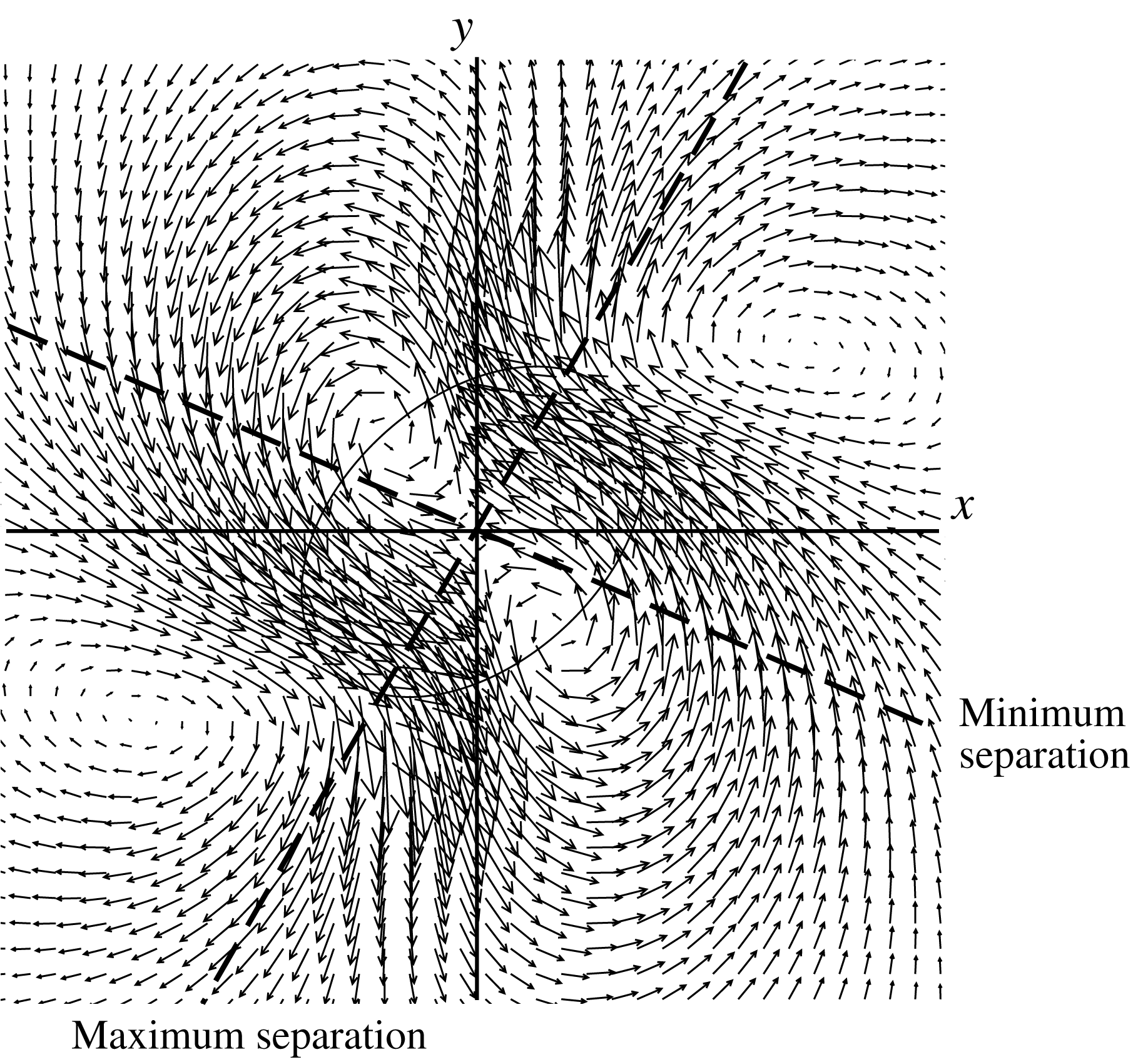
The second is the viscous sweeping effect, which favours drop attraction. Figure 13 shows the velocity field around a single ferrofluid drop spinning in a rotating field. We examine how a second drop, placed in different positions relative to the first, would be pushed or pulled by the radial component of the flow field. We prefer this simpler flow to the two-drop velocity field of figure 8, as the latter varies according to the location and orientation of the drops, and the added complexity obscures the underlying physics. Here, the flow is steady as far as the rotating drop is concerned. For ease of discussion, we orient the
 $x$
and
 $y$
axes always at
 $\unicode[STIX]{x03C0}/4$
from the long axis of the drop. Thus, the flow field stays the same at different times, and the second drop will be placed at different angular locations at different times during its revolution.
The velocity field around a single ferrofluid drop spinning steadily in a rotating field (
 $f=1/80$
,
 $Bo_{m}=2$
,
 $\unicode[STIX]{x1D709}=1$
and
 $La_{m}=75$
). The dashed lines indicate locations where a second drop will be at maximum or minimum separation from the one shown during planetary motion.

We start by noting that the radial dipolar force vanishes if the second drop is placed on the
 $x$
or
 $y$
axes (
 $\unicode[STIX]{x0394}\unicode[STIX]{x1D703}=\unicode[STIX]{x03C0}/4$
or
 $3\unicode[STIX]{x03C0}/4$
, see (4.1)). Next, to follow the increase of the phase lag
 $\unicode[STIX]{x0394}\unicode[STIX]{x1D703}$
during planetary motion, we imagine the second drop moving clockwise around the first, starting from the first quadrant. As the second drop passes from above the
 $x$
axis to below it,
 $\unicode[STIX]{x0394}\unicode[STIX]{x1D703}$
increases past
 $\unicode[STIX]{x03C0}/4$
.
 $F_{r}$
changes from attractive to repulsive, suggesting a minimum in separation
 $D$
. Because of inertia, however, the minimum is attained further clockwise at an angle of approximately
 $0.13\unicode[STIX]{x03C0}$
below the
 $x$
axis. Similarly the farthest separation is at about
 $0.17\unicode[STIX]{x03C0}$
past the
 $y$
axis. The flow is mostly radially inward in the region around the minimum
 $D$
but outward in the region around the maximum
 $D$
. As a result, the second drop experiences stronger inward flow than outward flow during its revolution. Although the overall radial flux around a drop necessarily vanishes, viscous sweeping favours approach over separation on balance. Figure 10(b) provides direct evidence for this argument. Raising the driving frequency
 $f$
increases the spinning velocity of the drops and the strength of viscous sweeping, which results in closer separation between the drops.
Finally, the third effect is anisotropic viscous drag, illustrated by the diagrams in figure 14. The radial magnetic force is attractive when the phase lag
 $\unicode[STIX]{x0394}\unicode[STIX]{x1D703}$
has a small magnitude (below
 $\unicode[STIX]{x03C0}/4$
). As the drops approach, therefore, they present relatively small cross-sections to each other and thus have smaller viscous drag
 $F_{\unicode[STIX]{x1D702}}$
(figure 14
a). Conversely, the separation phase sees the drops oriented away from their line of centroids, and the large cross-sectional area induces more viscous drag (figure 14
b). Overall the anisotropic viscous drag favours drop attraction.
Illustration of anisotropic viscous drag. Magnetic attraction in (a) induces a smaller viscous drag
 $F_{\unicode[STIX]{x1D702}}$
than the magnetic repulsion in (b).

With the three effects in simultaneous action, we can rationalize the attainment of the limit separation
 $D_{s}$
. When the drops are initially far apart, the inertial overshoot effect is weak, and the anisotropic drag and viscous sweeping effect bring the drops closer together. If the initial separation
 $D_{0}$
is small, the inertial overshoot is amplified as the asymmetry between approach and separation becomes relatively larger. This mechanism prevails over viscous sweeping and anisotropic drag to push the two drops apart. The limit separation will be achieved when all effects are in balance.
Admittedly, the arguments above are mostly qualitative since it is difficult to quantify each factor and analyse their variation with parameters such as
 $f$
. For instance, when we reduce the magnetic Bond number
 $Bo_{m}$
in figure 9, the rounded shape of the drop reduces viscous sweeping and anisotropic drag, and hence should increase the limit separation
 $D_{s}$
. In the meantime, numerical results show that the inertial overshoot is also suppressed for the round drop, probably by the reduction in flow velocity. The outcome is that
 $D_{s}$
only increases slightly. We can rationalize the outcome thus, but cannot make the quantitative calculation to predict it.
4.3 Drop locking
Figure 15 shows a typical simulation in the drop-locking regime. Compared with the planetary motion of figure 6, the viscosity ratio and the initial separation
 $D_{0}$
are both smaller. The drops initially approach each other as if coalescing, and form a thin liquid film between them. Then the two rotate as one at the same angular velocity as the external field. The locked rotation lasts for about
 $1/2$
of a cycle before coalescence.
A typical simulation in the drop-locking regime, with snapshots showing the drops and magnetic field lines (
 $f=1/80$
,
 $Bo_{m}=2$
,
 $\unicode[STIX]{x1D709}=0.2$
,
 $La_{m}=75$
and
 $D_{0}=3.5$
). The letter
 $L$
marks the drop (or the end of the combined drop) initially on the left. See also movie 3 in the supplementary material online.

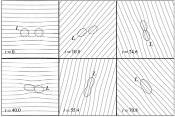
Intrigued by this behaviour, we went back to the laboratory to search for it experimentally (Lu Reference Lu2017). Indeed, starting with the conditions that would produce the planetary motion and gradually reducing the initial drop separation, we were able to confirm the drop-locking regime experimentally. Figure 16 shows snapshots of a pair of drops locked in close proximity and rotating with the driving frequency. In this case, the drops are locked for approximately 5/4 cycles of rotation before coalescing, a longer duration than in our numerical solution. This duration varies among experimental runs, apparently stochastically. In one extreme case, the drops remain locked for the entire duration of the experiment, for more than 12 cycles. In a sense, we can view drop locking as intermediate between planetary motion and direct coalescence. The transition among the regimes will be analysed in the next subsection.
Snapshots of drop locking observed in an experiment. The letter
 $L$
marks the drop (or the end of the combined drop) initially on the left. See also movie 4 in the online supplementary material.

The reason that drop locking lasts for a much shorter time in the simulations than in the experiment is likely twofold. First, we have used a lower viscosity for the surrounding medium in the simulations (see table 1), and this will produce faster film drainage. Second, insufficient numerical resolution of the thin liquid film between the drops may also lead to premature coalescence. As drop coalescence occurs upon rupturing of the thin liquid film separating them, its exact timing depends on molecular-scale forces and cannot be predicted by purely continuum models (Yue et al. Reference Yue, Feng, Liu and Shen2005). In simulations, therefore, rupture or coalescence is often precipitated by incidental factors such as numerical errors.
4.4 Transitions between regimes
The last section suggests that drop locking is an intermediate regime between planetary motion and direct coalescence. Naturally the question arises as to what conditions determine the transition between regimes. In § 4.1, we have found it convenient to describe the four regimes in terms of gradually reducing the initial separation
 $D_{0}$
. This is not the only way to organize the regimes. Now we will consider the transitions as the outcome of the various forces in competition.
Generally, the interaction of a pair of ferrofluid drops in a rotating field is determined by the competition between the magnetic forces and viscous drag. The former causes attraction and even coalescence, while the latter, by way of modifying the relative position and orientation of the drops, introduces the potential for repulsion and sustained cyclic motion without coalescence. Much insight can be gained from considering the simpler case of solid microspheres (or effectively magnetic dipoles) that has been studied before (Helgesen et al. Reference Helgesen, Pieranski and Skjeltorp1990; Bacri et al. Reference Bacri, Drame, Kashevsky, Neveu, Perzynski and Redon1995).
In this case, Helgesen et al. (Reference Helgesen, Pieranski and Skjeltorp1990) derived a critical driving frequency based on dipole interactions in three dimensions and the Stokes drag. Using our unit system and scaling (see § 2), this critical frequency can be written in dimensionless form as
 $$\begin{eqnarray}f_{c}=\frac{2\sqrt{La_{m}}}{\unicode[STIX]{x03C0}}\left(\frac{\unicode[STIX]{x1D712}}{3+\unicode[STIX]{x1D712}}\right)^{2}\frac{1}{D^{5}}.\end{eqnarray}$$
At a driving frequency
 $f<f_{c}$
, the magnetic force dominates the viscous drag. The pair rotates at the same speed as the driving field, with a phase lag
 $\unicode[STIX]{x0394}\unicode[STIX]{x1D703}$
never exceeding
 $\unicode[STIX]{x03C0}/4$
. Thus the magnetic radial force remains attractive at all times and the spheres approach each other and then stay in contact. This behaviour is the counterpart of our drop-locking regime. When
 $f>f_{c}$
, the strong viscous drag causes the phase lag
 $\unicode[STIX]{x0394}\unicode[STIX]{x1D703}$
to exceed
 $\unicode[STIX]{x03C0}/4$
. The two spheres periodically repel and separate, and revolve around each other at a lower rate, as in our planetary motion. Helgesen et al. (Reference Helgesen, Pieranski and Skjeltorp1990) and Bacri et al. (Reference Bacri, Drame, Kashevsky, Neveu, Perzynski and Redon1995) have also verified the predictions by experiments.
Extending this idea to the ferrofluid drops in our case, we can view the transitions outlined in figure 5 in a more general light. Increasing the initial separation
 $D_{0}$
tends to decrease the magnetic forces relative to the viscous drag, resulting in the shift from direct coalescence to drop locking, and further to planetary motion and independent spin. The same outcome can also be achieved by one or a combination of the following means: gradually increasing the driving frequency
 $f$
, reducing the magnetic susceptibility
 $\unicode[STIX]{x1D712}$
or reducing the magnetic Laplace number
 $La_{m}$
. In fact, as
 $La_{m}$
decreases from 75 to 50 in the simulation of figure 15, drop locking gives way to planetary motion. Furthermore, taking the experimental parameters of Chen et al. (Reference Chen, Hsueh, Wang and Li2015), equation (4.2) predicts the dimensional critical driving frequency to be 0.5 Hz. This is consistent with observations of the planetary motion at a driving frequency of 1 Hz in the experiment.
To make direct comparison with our 2-D numerical simulation, we assume Oseen flow with small inertia to avoid the singularity of Stokes flow. Balancing the dipole force in the azimuthal direction with the Oseen drag on a cylinder (Lamb Reference Lamb1911), we can derive a 2-D counterpart of (4.2):
 $$\begin{eqnarray}\frac{f_{c}}{\ln \left({\displaystyle \frac{3.7}{\unicode[STIX]{x03C0}D\sqrt{La_{m}}f_{c}}}\right)}=\frac{\sqrt{La_{m}}}{\unicode[STIX]{x03C0}}\left(\frac{\unicode[STIX]{x1D712}}{2+\unicode[STIX]{x1D712}}\right)^{2}\frac{1}{D^{4}}.\end{eqnarray}$$
In our numerical simulations, planetary motion prevails at a frequency of
 $f=0.025$
at
 $D_{0}=3.5$
,
 $La_{m}=75$
,
 $\unicode[STIX]{x1D712}=2$
and
 $\unicode[STIX]{x1D709}=0.2$
. Drop locking is realized at the lower frequency of
 $f=0.0125$
. Thus, the threshold frequency lies between these two values. Using the same parameters, equation (4.3) predicts a critical frequency of
 $f_{c}=0.0075$
, smaller than but of the same order of magnitude as the threshold frequency in the simulations.
Of course, our ferrofluid drops are not point dipoles, and their deformation and hydrodynamic interaction introduce new mechanisms into the picture. For one, we have observed that near the boundary between regimes, the initial positioning of the drops relative to the field can influence which behaviour prevails. In all the simulations presented so far, the drops are initially aligned along the field direction (horizontal in figure 2). Thus, the two drops initially attract and approach each other. If the two drops are placed in a vertical line, perpendicular to the initial field direction, they repel each other at the start. For a relatively close
 $D_{0}=3.6$
(the other parameters being
 $f=1/120$
,
 $Bo_{m}=2$
,
 $\unicode[STIX]{x1D709}=1$
,
 $La_{m}=75$
), we have observed the two drops coalescing directly from the horizontal initial configuration, but separating and settling into a planetary motion from the vertical initial configuration. In addition, the viscosity ratio
 $\unicode[STIX]{x1D709}$
of the ferrofluid to the surrounding medium affects the regimes. In the drop-locking example of § 4.3, increasing
 $\unicode[STIX]{x1D709}$
from
 $0.2$
to 1 while keeping all other parameters the same will cause a transition from drop locking to planetary motion. Increasing the viscosity of the ferrofluid drop makes it more rounded, and the reduced viscous sweeping tends to keep the drops farther apart. These are manifestations of the ferrofluid drop dynamics as distinct from that of magnetic dipoles.
A still more important factor is viscous sweeping, which can affect the drop interaction significantly. On the one hand, it directly promotes the revolution of the drops around each other through viscous forces. On the other, it tends to push the drops toward each other, magnifying the magnetic forces in the meantime. Thus, it is difficult to express its effects, say, as an algebraic generalization of (4.3). Given the computational cost, especially associated with resolving thin films, we have not undertaken a comprehensive parameter sweep to determine more precisely the boundaries among the regimes as part of this study.
5 Conclusion
Inspired by the experimental observations of Chen et al. (Reference Chen, Hsueh, Wang and Li2015), we have used direct numerical simulation to investigate the interaction between a pair of ferrofluid drops suspended in an immiscible fluid inside a rotating uniform magnetic field. The driving field is of sufficiently low frequency that the drops elongate and spin in phase with the field. We have observed four regimes of pairwise interaction within the range of parameters explored: independent spin, planetary motion, drop locking and direct coalescence. These are in qualitative agreement with experimental observations.
Furthermore, we have probed the mechanisms behind these outcomes by interrogating our numerical results. The transition between these regimes can be understood as the outcome of the competition of two types of forces: magnetophoretic forces that tend to attract the drops toward each other, and viscous drag that hinders the drop motion and causes the drops to fall periodically into a configuration of mutual repulsion. Thus, relatively strong magnetic forces favour coalescence, while relatively strong viscous drag favours less interactive regimes. The drop-locking regime was discovered in the simulations first, and then confirmed by new laboratory experiments. It represents an intermediate state between direct coalescence and planetary motion.
We have analysed the planetary motion in detail. A model of magnetic dipolar interaction explains well the oscillations in the trajectory of the drops. Although the magnetic interaction can also produce revolution of the two drops around each other, we have found a type of hydrodynamic interaction – viscous sweeping – to play a more important role. When an elongated drop spins with the driving field, it produces a flow field that sweeps the second drop in the same direction. As a result, drop interaction presents novel features that cannot be explained by dipolar interaction. For example, the average angular velocity of the planetary revolution increases with the driving frequency, contrary to predictions of the dipole model. Besides, the drops in planetary motion approach a mean separation in time that is independent of initial separations. This limit separation is smaller if the external field rotates faster.
We should note that the simulations are limited by computational cost to two dimensions, so quantitative comparison with experiments is difficult. The main numerical challenge comes from resolving the thin film between two drops. The solution for the magnetic field and the need for a large enough domain to avoid boundary interference also add to the magnitude of a full 3-D simulation. The main contribution of this study, therefore, consists in elucidating qualitatively the mechanisms underlying the experimental observations of ferrofluid drops in a rotating magnetic field. In this regard, the 2-D predictions match well with the experimental observations, including the transition between regimes (§§ 4.1 and 4.4) and the emergence of drop locking (§ 4.3). This indicates that the 2-D simulations have captured the essential physics. Beyond the pairwise interaction studied here, the experiments have also demonstrated self-organization of a cluster of drops into regular patterns (Chen et al. Reference Chen, Hsueh, Wang and Li2015). This, together with a full 3-D numerical calculation using more realistic material parameters, presents challenges for future theoretical and computational studies.
Acknowledgements
This work was supported by the Natural Sciences and Engineering Research Council (Canada), the Ministry of Science and Technology (Taiwan, ROC, grant no. MOST 104-2221-E-009-142-MY3) and the National Science Foundation (USA, grant no. NSF-CBET-1604351). The computation used the Extreme Science and Engineering Discovery Environment (XSEDE) supported by the National Science Foundation (USA grant no. ACI-1548562). M.Q. is also grateful for a Four-Year Doctoral Fellowship from the University of British Columbia. Effort by Mr Chun-Yi Lu in conducting ferrofluid drop experiments is greatly appreciated.
Supplementary movies
Supplementary movies are available at https://doi.org/10.1017/jfm.2018.261.