


I. INTRODUCTION
Neutron powder diffraction is a useful and complementary tool when compared with X-ray diffraction. For example, elements in the periodic table do not show atomic number dependence as is seen for X-rays. Neutron scattering factors contain scalar scattering lengths instead of atomic scattering factors that are angular dependent. In addition, neutron scattering contrast is isotope dependent. Unlike standard laboratory X-ray sources, nuclear research reactors and pulsed neutron sources are sited at national facilities (available worldwide). The particular interest of this paper is the use of high-resolution powder techniques available at pulsed neutron sources.
Calculated powder patterns have proved to be an invaluable asset in materials analysis (Clark et al., Reference Clark, Smith and Johnson1973; Smith and Smith, Reference Smith and Smith1986; Faber and Fawcett, Reference Faber and Fawcett2002; Faber, Reference Faber2004). The case for on-the-fly calculated constant wavelength (CW) neutron diffraction patterns has been published (Faber et al., Reference Faber, Crowder, Blanton, Kabekkodu, Gourdon, Blanton and Fawcett2014). For neutron time-of-flight (TOF), a brief recently published report (Faber et al., Reference Faber, Kabekkodu, Blanton, Blanton and Fawcett2017) showed on-the-fly powder pattern calculation and developed I/I c for TOF quantitative multiphase analysis. Here, we continue this development to calculate the background contribution for full patterns.
Historically, background contributions to experimental full patterns have been modeled using parameterized, empirically derived background functions. Many programs that calculate powder patterns completely ignore background contributions. In this paper, we will show that the rigor of TOF data reduction allows us to calculate a background function that contains contributions from isotope incoherent scattering and thermal diffuse scattering (TDS). This model will be tested using experimental data from reference standards typically used to calibrate the behavior of neutron TOF instruments. After the structure is defined, the powder pattern can be calculated and the proposed background model can be calculated without requiring additional parameters. The strategy for carrying out these goals requires us to refine the structural detail contained in the Bragg scattering. In the next section, we describe the TOF relations that are required to carry out these calculations.
II. TOF RELATIONSHIPS
For neutron TOF, the relationship between the d-spacing for a particular Bragg peak and its TOF are described by:
 $$t({\rm microseconds}) = {\rm DIFC} \;\bullet\; {\rm} d{\rm \;+\; DIFA} \;\bullet\; {\rm} d^2 {\rm \;+\; ZERO}$$
Given the flight path in the instrument (source to detector), the time for any particular neutron wavelength can be obtained from Eq. (1). The calibration constants, DIFC, DIFA, and ZERO are defined by instrument calibration. The Bragg scattering d-spacings then define the TOF. We have chosen to use the Thompson et al. (Reference Thompson, Cox and Hastings1987) profile function as described by:
 $$\eqalign{ H(\Delta t) = &(1 - \eta )N\left[ {e^u erfc(y) + e^v erfc(z)} \right] \cr &- \displaystyle{{2N\eta} \over \pi} \left\{ {{\mathop{\rm Im}\nolimits} \left[ {\exp (\,p)E_1 (\,p)} \right] + {\mathop{\rm Im}\nolimits} \left[ {\exp (q)E_1 (q)} \right]} \right\}}$$
where the first term involves the convolution of a Gaussian with leading and lagging exponentials. The second term creates a Lorentzian component in the peak shape. The parameters for the Gaussian and Lorentzian components can be used to characterize crystallite particle size and strain.
In addition,
 $$\Delta t = t - t({\rm peak}),\;E_1 {\rm is}\;{\rm defined}\;{\rm as}\;{\rm an}\;{\rm exponential}\;{\rm integral}$$
 $$\eqalign{p &= - \alpha \Delta t + \displaystyle{{i\alpha \gamma} \over 2}\quad {\rm and}\quad q = - \beta \Delta t + \displaystyle{{i\beta \gamma} \over 2} \cr u &= \displaystyle{\alpha \over 2}\left( {\alpha \sigma ^2 + 2\Delta t} \right){\rm,} \;v = \displaystyle{\beta \over 2}\left( {\beta \sigma ^2 - 2\Delta t} \right){\rm,} \cr y &= \; \displaystyle{{\alpha \sigma ^2 + \Delta t} \over {\sqrt {2\sigma ^2}}} {\rm,} \;z{\rm \;=\;} \displaystyle{{\beta \sigma ^2 + \Delta t} \over {\sqrt {2\sigma ^2}}} \cr \alpha =\, &\alpha _1 /d,\;\beta = \beta _0 + \beta _1 /d^4, \;\sigma ^2 = \sigma _0^2 + \sigma _1^2 d^2 + \sigma _2^2 d^4, \cr \;\gamma &= \gamma _0 + \gamma _1 d + \gamma _2 d^2} $$
The details of these parameters and equations are spelled out in the GSAS Technical Manual (Larson and Von Dreele, Reference Larson and Von Dreele2000; Toby, Reference Toby2001). An important point is that for each Bragg peak, the integral of the profile function, H, is defined by
 $\int {H(\Delta t)} = 1.0$
, which means that the calculated integrated intensity is distributed over all the points in the profile function. To take into account the Bragg peak broadening resulting from isotropic strain and sample broadening,
 $$\eqalign{S =\; & \displaystyle{1 \over C}\sqrt {(8\ln 2)(\sigma _1^2 - \sigma _{1i}^2 )} 100\% \;{\rm and} \cr P =\; & \displaystyle{{CK} \over {\gamma _2}}} $$
where S is the strain at full-width-at-half-maximum, P is the size parameter, K is the Scherrer constant (here assumed to be 1.0), and C is the diffractometer C value given above. For cylindrical neutron TOF powder diffraction (Bacon, Reference Bacon1975a), the integrated intensity is
 $$P = i(\lambda )\left( {\displaystyle{{\lambda ^4 l_s} \over {8\pi r}}} \right)\left( {\displaystyle{{V\rho ^{\prime}} \over \rho}} \right)\left( {\displaystyle{{\,jN_c^2 F^2} \over {2\sin ^3 \theta}}} \right)e^{ - 2W} A_{hkl} $$
where i(λ) is the incident flux on sample as a function of wavelength. Substituting Bragg's Law, and defining the scattering per unit cell:
 $$P = i(\lambda )\left( {\displaystyle{{l_s} \over {\pi r}}} \right)\left( {\displaystyle{{\rho ^{\prime}} \over \rho}} \right)\sin \theta \left( {\displaystyle{{\,jF^2 d^4} \over {V_{{\rm cell}}}}} \right)e^{ - 2W} A_{hkl} $$
In Eq. (5), there exists a d 4 term, which means that large d-space reflections are stronger than one might anticipate (recall that because the flux-on-sample has a Maxwellian component in the thermal region, the flux at large d-spaces would be expected to fall off in intensity). Note that for a pulsed source, a cold moderator would alter this expectation.
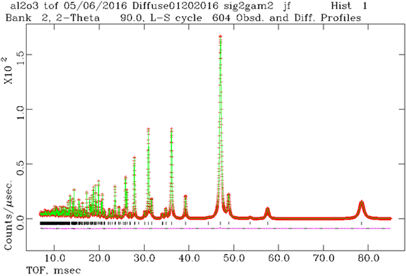
Given these relationships, we can proceed to calculate TOF full patterns. The program is called TOFtchDiffuseTDSabs09222016. After generating the digitized powder pattern, we have analyzed and checked the results using GSAS (Larson and Von Dreele, Reference Larson and Von Dreele2000; Toby, Reference Toby2001). In principal, we expect a perfect match between the pattern calculated with Powder Diffraction File (PDF)-4+ and the least-squares structural refinement carried out in GSAS. Consider Al2O3, with strain defined by S = 0.05 and size defined by P = 300 Å [see Eq. (3)]. These correspond to profile parameters, Δσ 2 = 23 and γ 2 = 75.3 for POWGEN (bank = 2) at the SNS. The result from the program “liveplot” in GSAS is shown in Figure 1.
(Color online) Results from GSAS using the combination of strain and size as given above. The Bragg peaks at largest TOF values show Lorentzian tails that arise from the size model. The pluses are the calculated data points, the solid green line connects the points for the theoretical model, the vertical tic marks define the Bragg peak positions, and the difference plot is shown below the tic marks.

The GSAS least-squares results give Δσ 2 = 23.1(9) and γ 2 = 75.3(1). As shown by the difference plot in Figure 1, the agreement between theory and structural refinement least-squares results are excellent. This gives a simple facility to simulate the effects of crystallite size and strain. These can then be compared with experimental data.
In Figure 1, we see that at large TOF, the Bragg peaks are clearly separated from the background, whereas at low TOF, the background appears to increase. In this case, the heuristic background fit was done with a series of Chebychev polynomials and the solution values we obtain with least-squares fit to the data using GSAS. The question that arises is: is the increase in scattering at low TOF due solely to instrumental background effects? Or could part of the rise be because of increasing overlapped Bragg reflections at low TOF?
III. RESOLUTION COMPARISONS
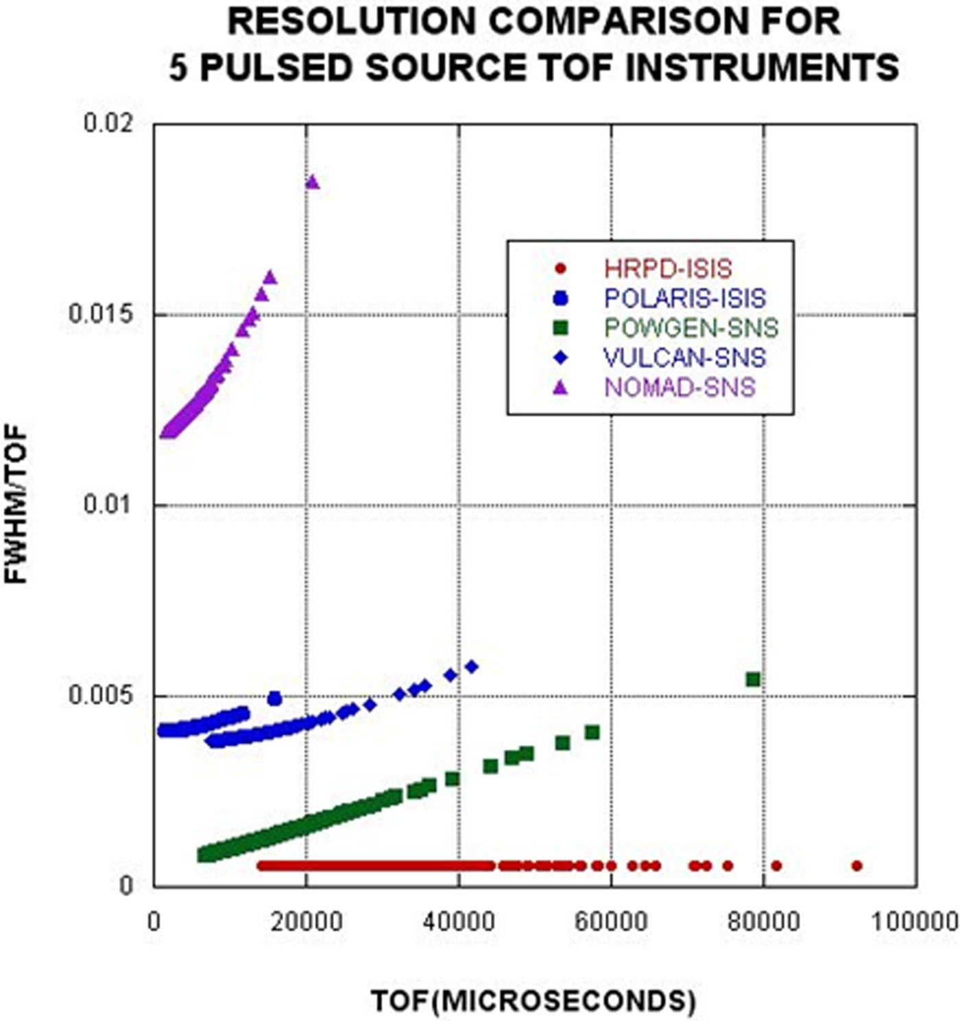
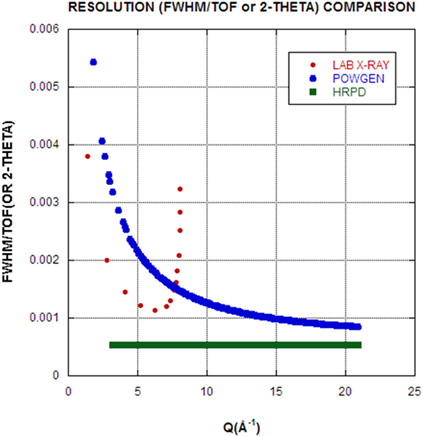
The ability to calculate TOF on-the-fly powder patterns means that we can calculate resolution functions for any TOF instrument provided that the associated instrument parameter file is available. To illustrate this capability, a resolution comparison is shown in Figure 2. For TOF profile coefficients, σ 2 terms have a d 4 dependence that produces increasing FWHM values at large TOF (large d). This is the primary cause of the increased FWHM for POWGEN compared with HRPD. Perhaps more relevant for X-ray diffraction practitioners, Figure 3 shows the comparison between a stereotypical in-house laboratory powder diffractometer and TOF instruments. Notice that the abscissa has units of Q = 4 πsin θ/λ = 2π/d. The laboratory machine resolution is set for CuK α1,2 and thus has Bragg peak doublets, whereas the TOF machines have singlet Bragg peaks. Notice in Figure 3 that the range of Q space is greatly expanded for the TOF case. In fact, machines with even higher Qs are available at most pulsed neutron sources. Both HRPD and POWGEN also exhibit better resolution than a standard X-ray diffractometer (especially if one takes into account the doublet radiation in the X-ray case). In the case of POWGEN, notice that the best resolution occurs at high Q, or small d-spaces, precisely where the number density of Bragg reflections increases. Of course the Q range in the laboratory case could be extended using Mo or Ag radiation, at some loss in resolution. The focus of this paper is to examine the details of background contributions to the full patterns.
(Color online) Resolution comparison for five TOF diffraction instruments. Only two of these instruments, POWGEN and HRPD, are high-resolution powder diffractometers. The others have significantly high count rates and resolutions more suitable for in situ studies, time-dependent studies, or S(Q) studies of glass, liquids, and amorphous materials.

(Color online) Comparison of resolution, Δt/t or Δ2Θ/2Θ vs. Q. The current world-class leader in TOF neutron resolution is HRPD at the ISIS pulsed source.

IV. BACKGROUND CALCULATION FOR TOF POWDER DIFFRACTION
The data reduction scheme on POWGEN at SNS takes into account data from:
-
• the sample in a vanadium can,
-
• the vanadium sample in a vanadium can,
-
• an empty vanadium can, and
-
• background taken without the sample can in the beam.
With statistical fluctuation and low background, this gives rise to a reduced data spectrum that scatters above and below zero counts. However, GSAS does not handle non-positive-definite observed intensities (these are excluded points in the fit); the data are rescaled by adding a small offset to avoid this problem. However, when we calculate background, we need to see the unscaled background. In the standard data reduction, the data without offset can be retrieved.
The total elastic scattering of a polycrystalline element or compound (Bacon, Reference Bacon1975b) is given by:
 $${\rm Total}\;{\rm scattering} = \displaystyle{{\pi N_c} \over {2\kappa ^2}} \sum\limits_{hkl} {(4\pi F_{hkl}^2} d_{hkl} ) + \sum {\sigma ({\rm inc})} $$
The first summation is over all of the hkl sample reflections and the second is made over all the atoms in the unit cell. This expression corresponds to the CW neutron diffraction case. We express this relationship for TOF as:
 $${\rm Total}\;{\rm scattering} = {\rm scale}^*\left( {\sum\limits_{hkl} {(I_{hkl}} ) + \displaystyle{1 \over {4\pi}} \sum {\sigma ({\rm inc})}} \right)$$
The second term is the incoherent scattering cross-section per atom. This model is applicable for all materials and depends only on the elements present in the sample.
Part of the background receives contributions from inelastic TDS, and may be calculated from (Bacon, Reference Bacon1975c):
 $$I_{{\rm TDS}} = \sum {\left\{ {1 - \exp ( - 2W)} \right\}b^2} $$
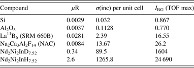
where W is the Debye factor, and b is the coherent scattering length. The summation is taken over the various atoms present. In this case, we have calculated the scattering contribution per unit cell, as was done in Eqs (6) and (7). We should note that Eq. (8) assumes a monoatomic solid, and therefore is an approximate expression to account for the effects of TDS. Table I shows calculated data for four compounds. Case-limiting calculated values of I BG are shown in the table, where I BG is the sum of the incoherent background and the I TDS.

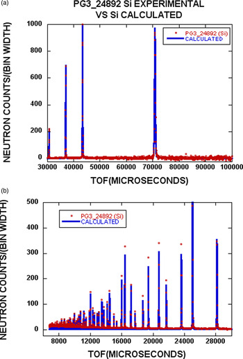
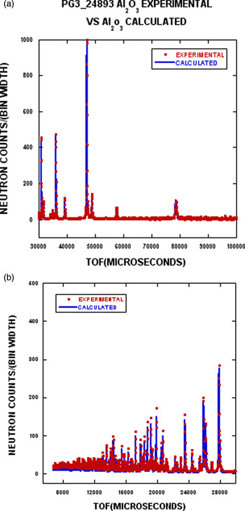
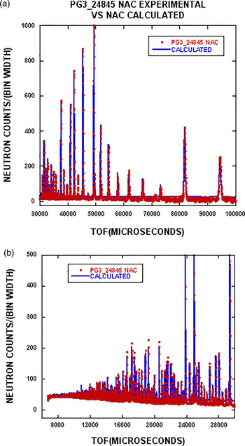
Corresponding to the compounds listed in Table I, the calculated and experimental results are shown in Figures 4–7. The experimental data are plotted for every second point to facilitate comparison between theory (solid line) and experiment (red points).
(Color online) The experimental data for Si from POWGEN are shown as the red dots, whereas the blue line represents the calculated profile including background [see Eqs (7) and (8)]. Figure 4(a) shows the TOF range from 30 000–100 000 µs). The data have been normalized to 1000 for the strongest reflection. In Figure 4(b), intensities have been magnified by a factor of two, and the TOF range is 6000–30 000 µs. The scales in Figures 5–7 are treated in the same way.

(Color online) The experimental data for Al2O3 from POWGEN are shown as red dots, whereas the blue line represents the calculated pattern including background.

(Color online) The experimental data for La11B6 (SRM 660b) from POWGEN are shown as red dots, whereas the blue line represents the calculated pattern including background.

(Color online) The experimental data for NAC from POWGEN are shown as red dots, whereas the blue line represents the calculated pattern including background.

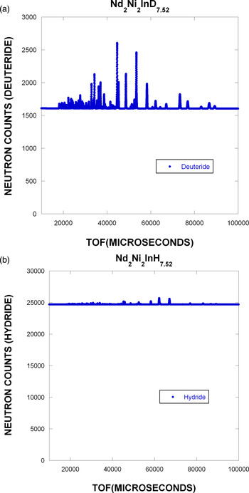
To demonstrate the calculated model in a more extreme case, Figure 8 shows the calculated results for Nd2Ni2InD7.52 and Nd2Ni2InH7.52. We would expect the background to be high as a result of the incoherent scattering from hydrogen. In the case of the deuteride, there remains a substantial isotopic incoherent scattering that arises from indium.
(Color online) Comparison in full pattern calculated results for Nd2Ni2InD7.52 (a) and Nd2Ni2InH7.52 (b). Note that the zero of the ordinate is not suppressed to emphasize the incoherent background contribution. The Bragg peaks are normalized in both (a) and (b) to 1000.

V. DISCUSSION
To start the discussion, it is important to emphasize that the calculated patterns in Figures 4–7 were generated using a structural refinement based on GSAS results. However, once the structural detail in the coherent component of the pattern has been defined, no additional adjustable parameters to describe the background model are required. The TDS model is quite simple and would not be expected to fit the fine details of the TDS-derived background. However, the computation time to calculate the total background is minimized.
The predictions of the background model yield excellent results for Si (Figure 4) and Al2O3 (Figure 5). The only areas of disagreement are at low TOF, or high Q. This is just where the TDS correction becomes more important. From Figure 3, we see that the resolution at high Q is improved and there is a concomitant reduction in the Bragg peak intensities. This shows that defects in the fit are most likely because of an inadequate TDS model and not simply a resolution detail resulting from Bragg peak overlap.
It appears from Figure 6 that a systematic overestimate of the background for LaB6 is obtained. There are several possible ways for which this can occur. The σ(inc) per unit cell could be incorrect. From Table I, we see that the incoherent background, σ(inc) and uR are at least 10–20 times larger than for Si or Al2O3. This just points out that the relative contribution of the incoherent scattering is much larger for this compound when compared with Si (Figure 4) or Al2O3 (Figure 5). In the case of LaB6 (SRM 660A) (Faber and Suchomel, Reference Faber and Suchomel2014), there was evidence for non-stoichiometry and a small amount of second phase was detected (680 ppm wt.%). However, SRM 660C has replaced SRM 660A, and shows no evidence for these effects. The conclusion is that defects or second phase are probably not responsible for the differences in the background fit.
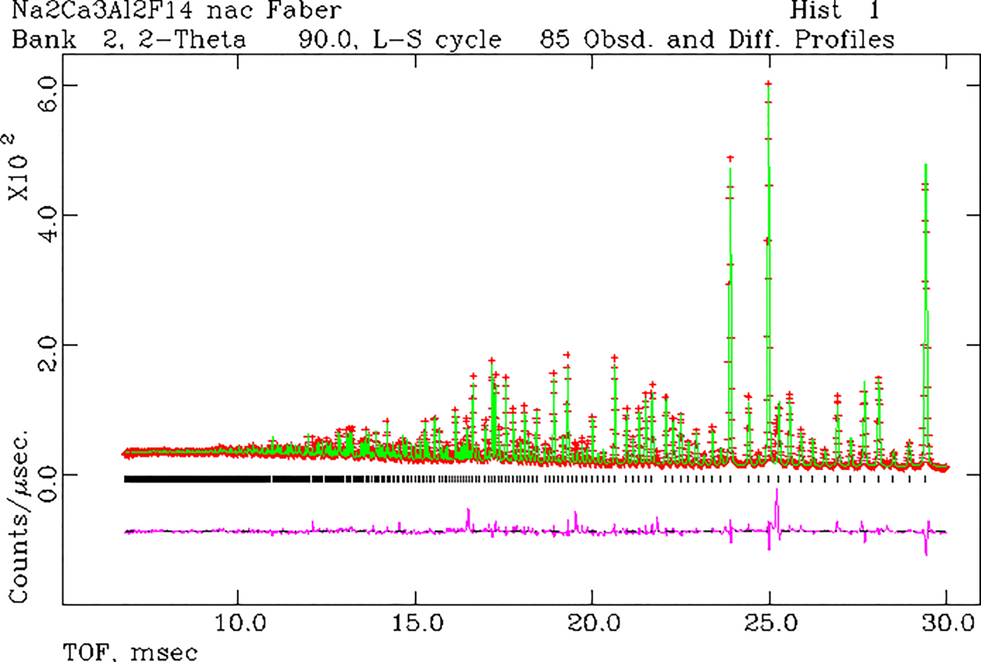
From Figure 7 for NAC, we see that there is a systematic overestimate in the incoherent background; however, the TDS (low TOF) seems to be in agreement. To focus on the background more than the Bragg scattering, only every second data point was plotted. However, we see that there is a cluster of experimental data points at ~43 000 µs that are clearly outside the bounds of this analysis. In a re-examination of the GSAS fit for NAC, Figures 9 and 10 show that there are several Bragg reflections that are observed and not accounted for in the model (in this case every experimental data point is plotted). Most notably, there are extra Bragg peaks at 43 193 and 71 229 µs. Using the ICDD PDF-4+ 2017, it is straightforward to show that these peaks correspond to CaF2. The experimental data are grouped in five histograms and quantitative phase analyses yielded the results in Table II. A particularly important point is that a second phase is almost always more sensitive to detection from neutron scattering when compared with X-ray scattering. Neutrons scatter from the entire volume of the sample, and the absorption cross-sections are much smaller and more uniform with respect to phase composition (shadowing of the minor phase by the major phase is essentially non-existent).
(Color online) Results of a single-phase GSAS refinement for NAC. In this figure, we show 30 > TOF > 100 ms.

(Color online) Results of a single-phase GSAS refinement for NAC. In this case, the range 7 < TOF < 30 ms is shown.

Simultaneous refinement of five histograms of experimental data on NAC using GSAS (Larson and VonDreele, Reference Larson and Von Dreele2000; Toby, Reference Toby2001). In this case, the focus is on a solution for the wt.% for the second phase, CaF2. The lattice parameter solutions are a(0) NAC = 10.2541(1) and a(0) CaF2 = 5.4661(1) Å. The reduced χ 2 = 9.5 for 25 211 observations.

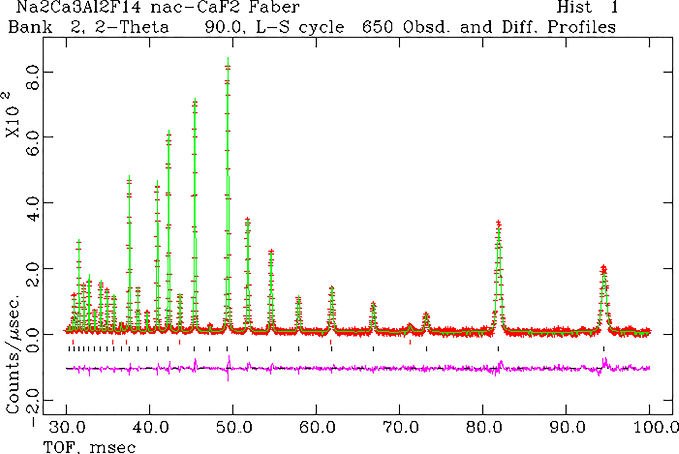
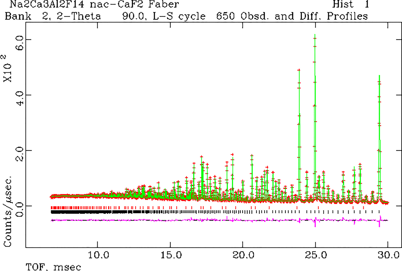
Choosing the arithmetic average of these results gives wt.% CaF2 = 2.8(2). For brevity, we show the two-phase solution for NAC by illustrating the GSAS results for histogram 1 in Figures 11 and 12.
(Color online) Rietveld refinement results for a two-phase model of NAC and CaF2. There is a substantial improvement in the fit after invoking a two-phase model. The red tic marks show the positions of the CaF2 peaks in the pattern. The black tics show the positions of the NAC Bragg peaks. In this figure, we show 30 < TOF < 100 ms.

(Color online) Rietveld refinement results for a two-phase model of NAC and CaF2. There is a substantial improvement in the fit after invoking a two-phase model. The red tic marks show the positions of the CaF2 peaks in the pattern. The black tics show the positions of the NAC Bragg peaks. In this figure, we show 7 < TOF < 30 ms.

A. The calculated background model
The calculated background model includes contributions from isotope incoherent scattering and TDS. Once the structural details are known (perhaps from Rietveld refinement), there are no additional parameters required to describe the background scattering. Agreement between theory and experiment for four standard reference compounds is quite good, despite the simplicity of the TDS model. The agreement between theory and experiment for NAC could be improved if a 50% reduction in the incoherent cross-section for Na was applied. Focusing on the experimental background led us to discover a detectable contribution from a second phase.
As anticipated, the calculated patterns for Nd2Ni2InD7.52 and Nd2Ni2InH7.52 in Figure 8 show huge contributions because of incoherent scattering. In this case, the contributions from TDS are overwhelmed by the incoherent scattering. It is perhaps interesting to note that there are four crystallographically independent H/D sites in the structure (orthorhombic Pbam). In this case, we need to be sure that the H/D substitution is complete (despite the possibility that the energetics of these four sites could be different). If D is not fully substituted for H, and provided that the individual sites are fully occupied, then the incoherent background will be a sensitive indicator for this condition. Alternatively, if a particular atomic site has mixed but random H/D occupation, then this will also affect the background level. The modeling of background thus becomes an important tool in assessing these cases. In a more complicated case, if short-range order between H/D site occupation occurs, then there will be a modulation of the TOF (or Q) dependence in the scattering. Beyond this example, there are many compounds (entries in the ICDD PDF-4+ 2017) that show incomplete substitution of H/D. One of the litmus tests for these effects is to model the total diffraction pattern consisting of Bragg peaks and background.
Another area of applicability for our model is in the determination of crystallinity, i.e. presence of amorphous structure and its characteristic scattering signature. The determination of crystallinity depends critically on an accurate determination of the background present in the diffraction pattern.
The rigorous attention to background as well as Bragg intensities and the approach described here is also applicable to X-ray scattering. In this case, the isotopic incoherent scattering disappears but fluorescence scattering must be calculated. Pulse-height discrimination must be carefully calibrated.
The experimental data show a need for improved statistics at large TOF. This limits the detection of weak second phases, ordered magnetic scattering, and weak paramagnetic diffuse scattering, all of which require accurate large TOF intensities. POWGEN's upgrade to improve the instrument performance was announced to start on January 2017 and should help remedy some of these shortcomings and better define the background detected. A report (Huq et al., Reference Huq, Hodges, Gourdon and Heroux2011) on the POWGEN instrument has been published.
ACKNOWLEDGEMENTS
The author acknowledges financial support from the ICDD for the calculation of TOF Bragg diffraction patterns. The author is pleased to acknowledge the help of Ashvia Huq (Instrument Scientist for POWGEN at the SNS, Oak Ridge National Laboratory) who made available the experimental powder data without the small background offset. The SNS is a DOE Office of Sciences User Facility operated by the Oak Ridge National Laboratory. In addition, the author gratefully received a release to use three specific Fortran routines, expint.for, epsvoigt. for and hfunc.for in connection with our code writing for on-the-fly TOF calculation via a personal communication (Von Dreele, R. B. On March 5, 2015).