1. Introduction
Barchan dunes are three-dimensional bedforms that typically form under flows characterized by limited directional variability and sediment supply. Most traditionally associated with dry aeolian environments (Finkel Reference Finkel1959; Livingstone, Wiggs & Weaver Reference Livingstone, Wiggs and Weaver2007; Elbelrhiti, Andreotti & Claudin Reference Elbelrhiti, Andreotti and Claudin2008; Smith, Jackson & Cooper Reference Smith, Jackson and Cooper2017), barchans represent a ubiquitous wind-driven landform typology on planetary surfaces, including Mars (Bourke Reference Bourke2010). Recent technological advances in bathymetric surveying have revealed their presence under water, in river channels (McCulloch & Janda Reference McCulloch and Janda1964; Carling et al. Reference Carling, Golz, Orr and Radecki-Pawlik2000; Kleinhans et al. Reference Kleinhans, Wilbers, De Swaaf and Van Den Berg2002) and on continental shelves (Todd Reference Todd2005; Ma, Yan & Fan Reference Ma, Yan and Fan2014; Couldrey et al. Reference Couldrey, Benson, Knaapen, Marten and Whitehouse2020). The crescentic planform shape of barchan dunes has been the focus of study for many decades (e.g. Hesp & Hastings Reference Hesp and Hastings1998; Sauermann et al. Reference Sauermann, Rognon, Poliakov and Herrmann2000), with a relatively large body of research aimed at understanding the flow–form–transport feedbacks that control their formation and evolutionary processes (e.g. Lancaster et al. Reference Lancaster, Nickling, McKenna Neuman and Wyatt1996; Wiggs, Livingstone & Warren Reference Wiggs, Livingstone and Warren1996; Baddock, Wiggs & Livingstone Reference Baddock, Wiggs and Livingstone2011; Weaver & Wiggs Reference Weaver and Wiggs2011; Yuxiang et al. Reference Yuxiang, Hesp, Dequan and Namikas2017). These bedforms are known to migrate at rates inversely proportional to their size (Andreotti, Claudin & Douady Reference Andreotti, Claudin and Douady2002; Hersen Reference Hersen2005), such that, within a field of barchans of varying size, dune–dune collisions are common. Barchan collisions, and bedform interactions more generally, have been studied both numerically (e.g. Katsuki et al. Reference Katsuki, Kikuchi, Nishimori, Endo and Taniguchi2011; Omidyeganeh et al. Reference Omidyeganeh, Piomelli, Christensen and Best2013; Parteli et al. Reference Parteli, Durán, Bourke, Tsoar, Pöschel and Herrmann2014; Wang & Anderson Reference Wang and Anderson2018) and experimentally (e.g. Endo, Taniguchi & Katsuki Reference Endo, Taniguchi and Katsuki2004; Hersen & Douady Reference Hersen and Douady2005; Fernandez, Best & López Reference Fernandez, Best and López2006; Palmer et al. Reference Palmer, Mejia-Alvarez, Best and Christensen2012; Bristow et al. Reference Bristow, Blois, Best and Christensen2018; Assis & Franklin Reference Assis and Franklin2020). Water tunnels, in which relatively small barchans ( $H\sim O(10^{-2}\ \textrm {{m}}$), where
 $H$ is the dune height) can easily be formed and allowed to evolve naturally over sufficiently short time scales, are commonly used to observe the morphological changes produced by these interactions (Endo et al. Reference Endo, Taniguchi and Katsuki2004; Hersen & Douady Reference Hersen and Douady2005; Assis & Franklin Reference Assis and Franklin2020). Longer time-scale observations via remote sensing of much larger and more complex aeolian barchan fields have also been critical to validation of theoretical, numerical and experimental findings (Ewing & Kocurek Reference Ewing and Kocurek2010; Vermeesch Reference Vermeesch2011; Hugenholtz & Barchyn Reference Hugenholtz and Barchyn2012; Hugenholtz et al. Reference Hugenholtz, Levin, Barchyn and Baddock2012).
Recent studies have increasingly shown that the morphodynamics of interactions between dunes in close proximity is linked to enhanced turbulence produced in the wake of an upstream bedform impinging on a downstream bedform (Fernandez et al. Reference Fernandez, Best and López2006; Wang et al. Reference Wang, Tang, Bristow, Blois, Christensen and Anderson2017; Bristow et al. Reference Bristow, Blois, Best and Christensen2018; Wang & Anderson Reference Wang and Anderson2018, Reference Wang and Anderson2019; Bristow et al. Reference Bristow, Blois, Best and Christensen2019, Reference Bristow, Blois, Best and Christensen2020; Assis & Franklin Reference Assis and Franklin2020; Bacik et al. Reference Bacik, Lovett, Colm-cille and Vriend2020; Khosronejad et al. Reference Khosronejad, Kang, Farhadzadeh and Sotiropoulos2020). Bacik et al. (Reference Bacik, Lovett, Colm-cille and Vriend2020) showed for transverse dunes that the turbulent wake of the upstream bedform influences the migration speed of the downstream bedform by enhancing downstream sediment flux. Assis & Franklin (Reference Assis and Franklin2020) demonstrated the role that other factors play in such interactions, including bedform alignment and sediment size and shape, while also emphasizing the importance of wake turbulence in the short-range interaction dynamics via a flow strength parameter. In coupled large-eddy simulations (LES) involving a deformable bed, Khosronejad et al. (Reference Khosronejad, Kang, Farhadzadeh and Sotiropoulos2020) recently showed that the morphodynamics of subaqueous barchanoid bedforms is strongly influenced by the hydrodynamics of the shear layer formed by upstream bedforms that propagate downstream. Bristow et al. (Reference Bristow, Blois, Best and Christensen2018, Reference Bristow, Blois, Best and Christensen2019, Reference Bristow, Blois, Best and Christensen2020), investigating the flow field associated with a collision sequence between fixed-bed, laterally offset barchans, showed how the mean flow, turbulence stresses, and secondary flows over the downstream dune are significantly altered by the approaching upstream dune. From this, they proposed that the morphological changes observed in naturally evolving barchans are controlled by turbulent processes. Wang et al. (Reference Wang, Tang, Bristow, Blois, Christensen and Anderson2017) and Wang & Anderson (Reference Wang and Anderson2018, Reference Wang and Anderson2019) studied similar collision configurations using LES, exploring additional flow features, including a flow channelling effect and hairpin vortex shedding, while also identifying the role of such features that persist in more complex barchan fields.
These advances in our understanding of bedform-scale dynamics and its interactions are complemented, and in part supported, by studies focusing on the links between turbulence and sediment transport at a granular scale. More specifically, instantaneous turbulent events above the transport threshold result in sediment motion (Williams & Kemp Reference Williams and Kemp1971; Grass Reference Grass1983; Best Reference Best1992; Nelson et al. Reference Nelson, Shreve, McLean and Drake1995; Roy et al. Reference Roy, Buffin-Belanger, Lamarre and Kirkbride2004; Pähtz et al. Reference Pähtz, Valyrakis, Zhao and Li2018; Cameron, Nikora & Marusic Reference Cameron, Nikora and Marusic2019; Cameron, Nikora & Witz Reference Cameron, Nikora and Witz2020; Li et al. Reference Li, Zhang, Herrmann, Shao and Huang2020). A common approach to identifying such ‘activating’ events is to decompose the near-bed Reynolds shear stress contributions into quadrants (Wallace, Eckelmann & Brodkey Reference Wallace, Eckelmann and Brodkey1972; Wallace Reference Wallace2016) based on positive and negative streamwise and wall-normal velocity fluctuations, and to correlate these with measurements of transport (e.g. Nelson et al. Reference Nelson, Shreve, McLean and Drake1995; Dwivedi et al. Reference Dwivedi, Melville, Shamseldin and Guha2011; Wiggs & Weaver Reference Wiggs and Weaver2012). Turbulent ‘sweep’ events, wherein higher-momentum fluid is swept downward to the bed, have been clearly linked to sediment mobilization. During a sweep event, drag and lift forces imparted by the fluid to the grains increase, producing periods of transport associated with the passage of these events. The spatio-temporal variability of these turbulent events is likely one of the main reasons why transport laws based only on mean flow quantities (e.g. mean bed shear stress) struggle to accurately predict transport, even for perfectly uniform sediment distributions (Barchyn et al. Reference Barchyn, Martin, Kok and Hugenholtz2014; Yager et al. Reference Yager, Venditti, Smith and Schmeeckle2018). Recent modifications of transport laws have revealed the effect of hysteresis in this regard, wherein the fluid threshold for transport must be exceeded to initiate saltation, but transport does not cease until the fluid forcing falls below the lower impact threshold (Martin & Kok Reference Martin and Kok2018; Comola et al. Reference Comola, Kok, Chamecki and Martin2019; Rana, Anderson & Day Reference Rana, Anderson and Day2020).
In addition to the intensity of a turbulent fluctuation, a key component of this momentum exchange mechanism is its duration. Seminal observations by Diplas et al. (Reference Diplas, Dancey, Celik, Valyrakis, Greer and Akar2008), accounting for both the intensity and duration of entrainment events, led to the development of the ‘impulse’ concept for sediment transport. This framework is based on the notion that the coherence of the turbulent flow motions is important, as the reaction of the sediment lags behind the fluid forcing due to particle inertia. Moreover, when the flow conditions approach the threshold of entrainment in terms of mean wall shear stress (i.e. incipient motion), the system becomes dynamic and each turbulent event must be considered independently (Celik, Diplas & Dancey Reference Celik, Diplas and Dancey2014). Fluctuations of instantaneous shear stress above the threshold will induce particle dislocation and could ultimately produce transport, if sustained for a sufficient duration.
Recently, Cameron et al. (Reference Cameron, Nikora and Marusic2019, Reference Cameron, Nikora and Witz2020) have shown that large- and very-large-scale motions (LSMs and VLSMs, respectively) in open channel flow are correlated with the entrainment of sediment. The presence of such motions, wherein VLSMs have been suggested to form by the streamwise concatenation of LSMs (Kim & Adrian Reference Kim and Adrian1999; Lee, Sung & Adrian Reference Lee, Sung and Adrian2019), is a hallmark of high Reynolds number (hereafter denoted as Re) wall turbulence (Kim & Adrian Reference Kim and Adrian1999; Balakumar & Adrian Reference Balakumar and Adrian2007; Hutchins & Marusic Reference Hutchins and Marusic2007a), present both in laboratory-scale flows as well as in the atmospheric surface layer (Hutchins et al. Reference Hutchins, Chauhan, Marusic, Monty and Klewicki2012; Wang & Zheng Reference Wang and Zheng2016). These LSMs and VLSMs (or ‘superstructures’, as the latter are often referred to in boundary layers) can sustain long durations of above-average streamwise momentum, while also modulating the amplitude and frequency of smaller-scale near-wall turbulence. The relatively recent discovery of superstructures means that their implications in terms of sediment transport are the subject of ongoing research (Cameron et al. Reference Cameron, Nikora and Witz2020).
While these studies focusing on near-bed turbulence physics provide the first evidence linking sediment transport to the larger-scale organization of wall-bounded turbulence, topographic effects such as roughness or bedforms will likely complicate this relationship. In the specific case of barchan dunes, field observations (Hersen, Douady & Andreotti Reference Hersen, Douady and Andreotti2002) suggest that they are generally immersed within the log layer of their characteristic formative flow. This scaling suggests that relative to the large streamwise extents of LSMs and VLSMs, individual barchan dunes can be viewed as isolated roughness elements. Studies that focus on flow over barchans in particular (i.e. capturing the relevant aspect ratio  $H/W$, where W is dune spanwise length), and which have also modelled bedforms at this scaling within the boundary layer, however, are relatively few (Palmer et al. Reference Palmer, Mejia-Alvarez, Best and Christensen2012; Wang et al. Reference Wang, Tang, Bristow, Blois, Christensen and Anderson2017; Bristow et al. Reference Bristow, Blois, Best and Christensen2018; Wang & Anderson Reference Wang and Anderson2018, Reference Wang and Anderson2019; Bristow et al. Reference Bristow, Blois, Best and Christensen2019, Reference Bristow, Blois, Best and Christensen2020). Moreover, these studies have generally not focused on how the boundary layer structure interacts with, and possibly modulates, the flow perturbations from the bedform itself.
While flow over an isolated barchan could be considered as similar to that considered in studies of flow around an idealized wall-mounted obstacle, such as a hemisphere, cube or cylinder, most such studies focus on scenarios wherein the wall-mounted obstacle occupies a substantial fraction of the boundary-layer thickness or even exceeds this in height (e.g. Acarlar & Smith Reference Acarlar and Smith1987; Martinuzzi & Tropea Reference Martinuzzi and Tropea1993; Manhart Reference Manhart1998; Pattenden, Turnock & Zhang Reference Pattenden, Turnock and Zhang2005; Wood et al. Reference Wood, De Nayer, Schmidt and Breuer2016). These flows differ significantly from cases where the obstacle extends only to the log layer of the turbulent boundary layer (up to  $H/\delta \approx 0.2$, where
 $\delta$ is the boundary layer thickness), at which point it is more appropriately viewed as a roughness element, exposed to much higher turbulence levels (Tomkins Reference Tomkins2001; Ryan, Ortiz-Dueñas & Longmire Reference Ryan, Ortiz-Dueñas and Longmire2011; Zheng & Longmire Reference Zheng and Longmire2014; Pathikonda & Christensen Reference Pathikonda and Christensen2015; Johnson et al. Reference Johnson, Thurow, Kim, Blois and Christensen2017; Tan & Longmire Reference Tan and Longmire2017; Tang et al. Reference Tang, Jiang, Zheng and Wu2016; Kim & Christensen Reference Kim and Christensen2018).
Many other studies have considered more distributed roughness, either as discrete roughness elements or more continuous surface morphologies that populate the entire wall, but still with a relatively large protrusion into the log layer (e.g. Coceal et al. Reference Coceal, Dobre, Thomas and Belcher2007; Guala et al. Reference Guala, Tomkins, Christensen and Adrian2012). In addition, extensive literature exists concerning more traditional rough-wall turbulence wherein the roughness is exposed to (and thus most directly perturbs) the inner region of the boundary layer (e.g. Raupach, Antonia & Rajagopalan Reference Raupach, Antonia and Rajagopalan1991; Jiménez Reference Jiménez2004), including recent efforts focused on multiscale, irregular topographies reminiscent of practical engineering systems (due to surface damage) (Wu & Christensen Reference Wu and Christensen2007; Anderson et al. Reference Anderson, Barros, Christensen and Awasthi2015) as well as geophysical landscapes (e.g. Anderson et al. Reference Anderson, Passalacqua, Porté-Agel and Meneveau2012). However, due to this difference in protrusion into the boundary layer, these latter studies are quite distinct from surface topography that extends deep into the log layer.
The studies of roughness elements most relevant to the work presented herein are those that focus on individual or tandem roughness elements immersed up to the log layer of a turbulent boundary layer, as opposed to widely distributed elements covering the entire wall. Most such studies considered hemispheres (Tomkins Reference Tomkins2001; Johnson et al. Reference Johnson, Thurow, Kim, Blois and Christensen2017) and cylinders (Ryan et al. Reference Ryan, Ortiz-Dueñas and Longmire2011; Pathikonda & Christensen Reference Pathikonda and Christensen2015; Tang et al. Reference Tang, Jiang, Zheng and Wu2016), which typically have aspect ratios of at least  $H/W=1$, where
 $H$ and
 $W$ are the obstacle height and spanwise length, respectively. Barchan dunes, in general, have very low aspect ratios of
 $H/W \approx 0.1$, with
 $H\sim O(10^{0} - 10^{1}\ \textrm {{m}})$ for aeolian barchans (Hersen et al. Reference Hersen, Douady and Andreotti2002),
 $H\sim O(10^{-2} - 10^{-1}\ \textrm {{m}})$ for barchans in rivers (Konsoer et al. Reference Konsoer, Rhoads, Best, Langendoen, Abad, Parsons and Garcia2016) and
 $H\sim O(10^{0}\ \textrm {{m}})$ on continental shelves (Todd Reference Todd2005; Ma et al. Reference Ma, Yan and Fan2014). As mentioned previously, barchan dunes are generally immersed within the log layer of their respective environments and therefore, although previous studies of cylindrical and hemispherical roughness elements immersed in the log layer are the most relevant to the work herein, they are certainly distinct from bedforms in terms of their geometry.
The aim of the present study is to elucidate the ‘hierarchical’ organization of, and interaction between, the dominant turbulent flow structures associated with barchan dunes. In particular, the existence of a link between coherent structures shed in the wake of the barchan and the larger structures transported in the overlying turbulent boundary layer within which barchan dunes are immersed is investigated. In addition, the role that this flow physics might play in barchan–barchan interactions and associated sediment transport processes is explored, for which bedform three-dimensionality and offset alignments are critical factors. As such, the present study combines knowledge of boundary-layer structure concerning the dynamics of vortex shedding from roughness elements, and the resultant turbulence statistics, in order to provide key insights into fundamental processes of planetary surface boundary layers.
2. Experimental methods
Experiments were conducted in the large-scale refractive-index-matching (LS-RIM) flow facility at the University of Notre Dame, described in detail in Blois et al. (Reference Blois, Bristow, Kim, Best and Christensen2020). The facility features a closed-loop, recirculating liquid-flow tunnel whose test section is  $0.45\ \mathrm {m}\times 0.45\ \mathrm {m}\times 2.5\ \textrm {m}$ in cross-section, with the full depth being filled with liquid for the experiments reported herein. The primary advantage of a RIM flow environment is the mitigation of surface reflections and optical aberrations from laser illumination in the presence of complex topography that are detrimental to near-surface particle image velocimetry (PIV) measurements. These effects are minimized when the refractive index (RI) of transparent barchan models matches that of the working fluid – effectively rendering the barchan models virtually invisible when immersed in the flow facility and permitting uninhibited optical access to the entire flow field surrounding the models. This capability is achieved in the LS-RIM through a combination of an aqueous solution of sodium iodide (
 ${\sim }63\,\%$ by weight, with specific gravity
 $c. 1.8$) as the working fluid and cast acrylic as the solid model material. To fine tune and maintain the fluid RI, the temperature of the working fluid is controlled via an in-line heat exchanger. Further details on this facility can be found in Blois et al. (Reference Blois, Bristow, Kim, Best and Christensen2020).
The solid barchan models and geometrical configurations investigated herein involved an isolated barchan and three representative collision cases (figure 1). These configurations match those reported in Bristow et al. (Reference Bristow, Blois, Best and Christensen2018, Reference Bristow, Blois, Best and Christensen2019, Reference Bristow, Blois, Best and Christensen2020), allowing straightforward comparisons with previous measurements. The upstream barchan in figure 1(b–d) is a scaled version of the isolated barchan (volumetric ratio between the two barchans is 1 : 8). The volume of the downstream barchan is maintained identical to the isolated case for all collisions, with its morphology unaltered in collision case A, while the horn aligned with the upstream barchan is elongated in collision cases B and C. As discussed in Bristow et al. (Reference Bristow, Blois, Best and Christensen2018), although these morphologies do not match exactly a specific barchan dune in nature, they represent a generic barchan morphology that is expected to be associated with a similar flow structure as most common barchan dunes. These collision configurations are idealizations inspired by the mobile bed experiments of Hersen & Douady (Reference Hersen and Douady2005) and simply seek to qualitatively represent the main evolutionary features observed in those experiments. As such, the downstream barchan dune horn in collisions B and C is elongated as a function of interdune separation based on measurements provided in the supplemental material of Hersen & Douady (Reference Hersen and Douady2005). The cast acrylic models are polished to have a smooth surface, similar to the acrylic walls of the test section. The reader is referred to Bristow et al. (Reference Bristow, Blois, Best and Christensen2018) for further details on the barchan morphologies adopted, as well as the method for fabricating the models.
The morphologies and configurations of the barchan dunes studied herein: (a) isolated case; (b–d) collision cases. Green lines mark streamwise positions of the spanwise–wall-normal measurement planes that were unchanged for all configurations. (e) Shows a streamwise–wall-normal (x–y) view of the isolated barchan; the mean slopes of the stoss and lee sides along the dune centreline are indicated by the red line. Adapted from Bristow et al. (Reference Bristow, Blois, Best and Christensen2018).

The specific experimental datasets presented herein were collected contemporaneously with those reported in Bristow et al. (Reference Bristow, Blois, Best and Christensen2020), which specifically involved a number of cross-plane stereo-PIV measurements. Herein, the analysis leverages a suite of high-frame-rate measurements for the same barchan model configurations and flow conditions discussed in Bristow et al. (Reference Bristow, Blois, Best and Christensen2020). Figure 1 illustrates the streamwise locations of the cross-planes in which PIV measurements were made.
Flow measurements were conducted in wall-normal–spanwise (y–z) planes (hereafter the cross-plane) at four fixed streamwise ( $x$) positions (see figure 1b) with a field of view (FOV) of
 $45\ \textrm {mm}\times 90\ \textrm {mm}$ (
 $y\times z$) using stereo PIV, which allowed all three velocity components to be captured (figure 2). The flow was seeded with silver-coated solid glass spheres (
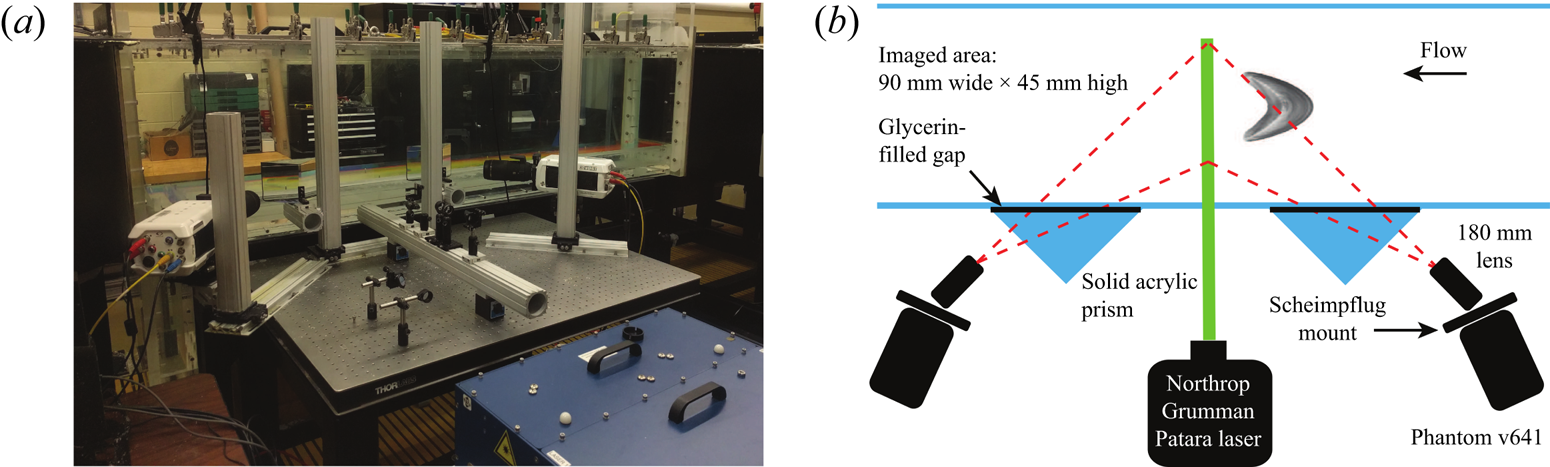
 $2\ \mathrm {\mu }\textrm {m}$ in diameter and specific gravity of 3.5) and illuminated with a Northrop Grumman, dual-cavity, Nd:YLF Patara laser. Image pairs were collected using two 4MP Phantom v641 cameras, fitted with 180 mm Sigma lenses and positioned on Scheimpflug mounts supplied by LaVision that viewed the same FOV but from opposite sides of the illuminating light sheet. Due to the high RI of the aqueous NaI solution (
 ${\approx }1.49 \ {\rm at} \ 20\,^{\circ}{\rm C} $), solid acrylic prisms were attached to the sidewall of the test section in order to compensate for the
 $45^{\circ }$ stereoscopic viewing angles. The air gaps between the prisms and the sidewall were filled with glycerin to minimize the discontinuity in RI along the imaging paths of the cameras.
(a) Photograph of the stereo-PIV experimental set-up in the LS-RIM; (b) top-view schematic representation of the stereo-PIV arrangement. Reproduced from Bristow et al. (Reference Bristow, Blois, Best and Christensen2020).

Figure 1 illustrates the locations of the y–z measurement planes for the datasets used herein related to each barchan configuration, as well as the dimensions of the models and their positions. Relative to the streamwise position of the crest of the isolated (or downstream) barchan ( $x/H=0$), data were collected from the interdune region at
 $x/H=-2.5$ (near the toe) and
 $x/H=-1$, and from the wake of the isolated (or downstream) barchan at
 $x/H=5$ and
 $x/H=6.5$, where
 $H$ is the height of the larger, downstream barchan. Measurement plane
 $x/H=5$ coincides approximately with the mean flow reattachment location at the centreline, based on the results of Bristow et al. (Reference Bristow, Blois, Best and Christensen2018). The FOV covered roughly
 $9.5H\times 4.7H$ in the spanwise and wall-normal directions, respectively. The final PIV interrogation window size of
 $16\times 16\ \textrm {pixels}^{2}$ and a 50 % window overlap yielded a grid spacing of approximately
 $220\ \mathrm {\mu }\textrm {m}$, or
 $0.023H$.
PIV image pairs were first acquired at each location at a low frame rate of 20 Hz (4 sets of 2700 image pairs), to enable uncorrelated ensembles for statistical calculations. Subsequently, image pairs were captured at higher frame rates of 350 Hz for the isolated barchan wake and 700 Hz for the interdune region (12 sets of 2700 image pairs). These latter measurements are the focus of the analysis presented herein.
The boundary layer at the inlet of the test section was tripped using a half-cylinder (7 mm in radius), resulting in a turbulent boundary layer thickness of  $\delta =52.5\ \textrm {mm}$ and a free-stream velocity,
 $U_e$, of
 $0.97\ \textrm {ms}^{-1}$ (obtained separately with PIV measurements over a larger FOV for the same flow conditions) at the measurement location (approximately 1.7 m downstream of the inlet at the centreline). Sidewall boundary layers are thinner, as they are not tripped upstream. Therefore, given the 0.45 m span of the test section and the 0.06 m width of the models, incoming flow is uniform across the span of the FOV. For the various tandem model configurations, the position of the light sheet was maintained fixed while the models were moved instead, which simplified the data collection. As the boundary layer is not undergoing rapid growth this far downstream, the varied positions of the models, depending on the measurement position within the model configuration, are not expected to introduce appreciable changes. The friction velocity was
 $u_{\tau } \approx 0.0380\ \textrm {ms}^{-1}$, found using both the Clauser chart method (Clauser Reference Clauser1954) and the boundary layer fitting method (Chauhan, Monkewitz & Nagib Reference Chauhan, Monkewitz and Nagib2009), resulting in a friction Reynolds number
 $Re_{\tau }=u_{\tau } \delta / \nu \approx 1800$, where
 $u_{\tau }$ is the friction velocity and
 $\nu$ is the fluid kinematic viscosity. Profiles of mean velocity,
 $\langle U \rangle$, and Reynolds stresses,
 $\langle u^{2} \rangle$,
 $\langle v^{2} \rangle$ and
 $\langle uv \rangle$, are shown in figure 3. In the following,
 $U$,
 $V$ and
 $W$ denote streamwise, wall-normal and spanwise velocity components, respectively, while lower-case velocities denote fluctuating quantities and brackets
 $\langle \cdot \rangle$ indicate temporal averaging. Comparisons of the smooth-wall boundary-layer profiles with LES (Eitel-Amor, Örlü & Schlatter Reference Eitel-Amor, Örlü and Schlatter2014) and hot-wire measurements (Örlü & Schlatter Reference Örlü and Schlatter2013) from similar Re show good agreement with canonical zero-pressure-gradient turbulent boundary layer statistics. The slightly weaker wake region in the present mean-velocity results compared to that from the literature is associated with a slight favourable pressure gradient imposed by the constant cross-sectional area of the LS-RIM test section. Based on separate PIV experiments measuring the free-stream velocity gradient across a 160 mm long x–y plane (centred at the same 1.7 m downstream position relative to the inlet), the Clauser pressure gradient parameter is
 \begin{equation} \beta=\frac{\delta^{*}}{\tau_w}\frac{\mathrm{d}P}{\mathrm{d} x}={-}\frac{\delta^{*}}{u_{\tau}^{2}}U_e\frac{\mathrm{d}U_e}{\mathrm{d} x}\approx{-}0.1, \end{equation}
where P is pressure,  $\delta ^{*}$ is the displacement thickness and
 $\tau _w$ is the mean wall shear stress, and the acceleration parameter is
 \begin{equation} K = \frac{\nu}{U_e^{2}}\frac{\mathrm{d}U_e}{\mathrm{d} x}\approx 3\times 10^{{-}8}. \end{equation}
Both of these metrics confirm that the favourable pressure gradient present in the LS-RIM test section is mild, with  $K$ in the present work just above the nominally zero-pressure-gradient conditions reported by Flack, Schultz & Connelly (Reference Flack, Schultz and Connelly2007) in studies of roughness effects in turbulent boundary layers and two orders of magnitude smaller than that necessary to relaminarize the flow (Sreenivasan Reference Sreenivasan1982).
Incoming smooth-wall boundary-layer conditions, with comparisons to LES (Eitel-Amor et al. Reference Eitel-Amor, Örlü and Schlatter2014) and hot-wire (Örlü & Schlatter Reference Örlü and Schlatter2013) data from comparable Re. The model height  $H^{+}$ is indicated by the vertical line.

An important aspect in the design of the present experiments was the relation between the flume and the natural environment in which barchan dunes form. Atmospheric boundary layers typically feature Reynolds numbers  $Re_{\tau } \sim O(10^{6})$. Therefore, the log layer of the turbulent boundary layer (which thickens as Re grows) is relatively large, allowing the bedforms formed under such conditions to be fully immersed within this region. Due to the universality of the log layer, this means that the relevant scaling necessary to appropriately study flow over dunes in a laboratory setting is the immersion of the laboratory-scale model within the log layer of the laboratory turbulent boundary layer (i.e.
 $H/\delta < 0.2$, with
 $H^{+}$ indicated in figure 3). This scaling ensures that the relevant dynamical and statistical properties of the flow structure that are imposed on natural bedforms of similar morphology are sufficiently captured in a laboratory setting. In the current experiments, this condition is met since
 $H/\delta = 0.18$.
3. Results
Understanding the dynamics and spatial distribution of coherent flow structures populating the wake of a bedform is important, as these flow features are hypothesized to produce impulsive, sediment transport events that contribute significantly to bedform evolution (Nelson et al. Reference Nelson, Shreve, McLean and Drake1995; Diplas et al. Reference Diplas, Dancey, Celik, Valyrakis, Greer and Akar2008; Valyrakis, Diplas & Dancey Reference Valyrakis, Diplas and Dancey2013; Shih et al. Reference Shih, Diplas, Celik and Dancey2017; Amirshahi, Kwoll & Winter Reference Amirshahi, Kwoll and Winter2018; Cameron et al. Reference Cameron, Nikora and Witz2020; Schobesberger et al. Reference Schobesberger, Lichtneger, Hauer, Habersack and Sindelar2020). In the following, the high-frame-rate cross-plane data are used to examine the three-dimensional structure of the flow, using Taylor's hypothesis, to clarify the structural organization of turbulence produced by barchan dunes. The frequencies with which vortices are shed are then examined to document the dynamics of flow in the barchan wake and relate their physics to the overlying boundary-layer structure through amplitude modulation analysis (Mathis, Hutchins & Marusic Reference Mathis, Hutchins and Marusic2009; Baars et al. Reference Baars, Talluru, Hutchins and Marusic2015; Pathikonda & Christensen Reference Pathikonda and Christensen2017). These instantaneous flow features leave their imprint on the statistics of turbulent stresses, which will be further examined in terms of turbulent impulses associated with components of the Reynolds shear stress, both in the context of an individual isolated barchan as well as tandem barchan interactions.
3.1. Three-dimensional flow structure
3.1.1. Taylor's hypothesis
Taylor's hypothesis of frozen turbulence has been commonly applied to enable translation between dimensions in time and space (e.g. Hutchins & Marusic Reference Hutchins and Marusic2007a; Dennis & Nickels Reference Dennis and Nickels2008; Ganapathisubramani, Lakshminarasimhan & Clemens Reference Ganapathisubramani, Lakshminarasimhan and Clemens2008; Dennis & Nickels Reference Dennis and Nickels2011a,Reference Dennis and Nickelsb; Hutchins et al. Reference Hutchins, Monty, Ganapathisubramani, Ng and Marusic2011; Mejia-Alvarez, Wu & Christensen Reference Mejia-Alvarez, Wu and Christensen2014). The essence of the hypothesis is that if the convective velocities,  $U_c$, of coherent structures in the flow are much greater than the turbulent fluctuations in that same region of the flow, convective effects dominate over viscous ones. When such conditions exist, one may perform a space–time coordinate transformation,
 $x=-U_c t$, that converts temporal measurements from a fixed streamwise position to equivalent spatial data in the streamwise direction (Dennis Reference Dennis2009; Dennis & Nickels Reference Dennis and Nickels2011a). This approach is particularly useful when time-resolved cross-plane PIV measurements are available, allowing the concatenation of a series of planar velocity fields into a pseudo-three-dimensional volume, from which the three-dimensional (3-D) nature of flow events, like vortices, can be clarified. The application of Taylor's hypothesis, however, requires careful consideration of its limitations and the choice of an appropriate convection velocity.
The identification of an appropriate convection velocity is not necessarily straightforward. The simplest case in this regard is when the analysis is limited to measurements from a single wall-normal height in a spanwise-homogeneous boundary layer. A common approach in this case is to use the local mean velocity (e.g. Dennis & Nickels Reference Dennis and Nickels2008; Mejia-Alvarez et al. Reference Mejia-Alvarez, Wu and Christensen2014). However, when the full wall-normal profile is used, the local mean velocity varies with wall-normal location and introduces potential ambiguity. Del Álamo & Jiménez (Reference Del Álamo and Jiménez2009) showed that larger-scale structures in a spanwise-homogeneous boundary layer convect at a relatively uniform velocity that is close to the bulk velocity. Dennis & Nickels (Reference Dennis and Nickels2011a) applied this finding and used Taylor's hypothesis to reconstruct a 3-D flow volume from cross-plane PIV measurements by using a single (i.e. uniformly applied) convection velocity, equal to the bulk velocity (Dennis Reference Dennis2009). Hutchins et al. (Reference Hutchins, Monty, Ganapathisubramani, Ng and Marusic2011), using simultaneous hot-wire probe measurements at varying wall-normal heights, reconstructed 3-D conditionally averaged flow fields also using a single convection velocity. They argued that the large scales that reside in the log layer convect at a velocity corresponding with the mean streamwise velocity at the midpoint of the log layer, and supported this contention with correlations between probes in a streamwise array. In the present case, we are concerned primarily with structures of the order of the barchan height, which herein are hypothesized to form in the shear layer via vortex roll-up and convect downstream forming the barchan wake. This shear layer at the centreline emanates from the crest of the barchan where the flow separates, as shown by Bristow et al. (Reference Bristow, Blois, Best and Christensen2018) (figure 4a therein). As such, the most appropriate single convection velocity is expected to be close to the mean streamwise velocity at the height of the barchan and along the centreline ( $y/H=1$,
 $z/H=0$) in each cross-plane measurement location (
 $U(x/H=5)=0.39U_e, U(x/H=6.5)=0.46U_e$). As will be shown in § 3.1.3, a good approximation of the convection velocity, based on comparison with streamwise-resolved planar velocity ‘ground truth’ data in the streamwise–wall-normal plane, is found to be
 $U_c=0.3U_e$ at
 $x/H=5$ and
 $U_c=0.35U_e$ at
 $x/H=6.5$.
Lastly, it should be noted that Taylor's hypothesis assumes that the flow structures convecting through the measurement location do not undergo significant evolution as they pass – i.e. they remain ‘frozen’ and simply convect downstream. Work by Dennis & Nickels (Reference Dennis and Nickels2008) in a smooth-wall boundary layer showed that this assumption was valid up to convection distances of approximately  $6\delta$. In the present case, however, the streamwise velocity gradients that characterize flow recovery in the wake make application of Taylor's hypothesis for similarly large streamwise extrapolations untenable. It is also emphasized that the use of this approach herein is not meant as a quantitative assessment of flow structure but rather a qualitative one. However, the level of temporal coherence of streamwise vortices in the cross-plane can be directly measured. To do so, a feature tracking algorithm was applied to the instantaneous, in-plane flow fields.
The methodology of this algorithm involves applying a top-hat smoothing filter to instantaneous cross-plane flow fields, making it easier to identify the local maxima/minima associated with a desired flow feature from a peak-finding algorithm. For example, in identifying and tracking vortices, this means that the centres of swirling motions in the flow field are found by applying the filter and peak finding to the output of vortex-identification calculations. Swirling strength is used for this purpose and is computed as the imaginary component of the complex eigenvalue of the local velocity gradient tensor,  $\partial U_i/\partial x_j$ (Zhou et al. Reference Zhou, Adrian, Balachandar and Kendall1999; Adrian, Christensen & Liu Reference Adrian, Christensen and Liu2000; Chakraborty, Balachandar & Adrian Reference Chakraborty, Balachandar and Adrian2005). As a Galilean invariant measure of rotation in the flow,
 $\lambda _{ci}$ does not highlight regions of intense shear, unlike vorticity, but rather effectively isolates regions of pure rotation as vortex cores. Peak swirling strength locations are then tracked between time steps using an open-source particle tracking code implemented in MATLAB (Blair et al. Reference Blair, Dufresne, Crocker and Grier2008). Swirling strength naturally biases toward smaller-scale structures, however, and therefore a preliminary low-pass spatial filter was applied to the velocity fields prior to the top-hat smoothing filter in the peak-finding algorithm. This preliminary filter involved reconstructing vector fields via snapshot proper orthogonal decomposition (POD) (Sirovich Reference Sirovich1987), wherein 67 % of the total turbulent kinetic energy (TKE) is retained by removing higher mode numbers. This method filtered out smaller scales so that vortices associated with the barchan wake could be consistently identified and tracked.
This method was applied to track streamwise vortices within a cross-plane region approximating the bulk of the wake ( $z/H\in [-1.8,1.8]$,
 $y/H\in (0,1.5]$) at both measurement positions (
 $x/H=5, 6.5$). The probability distribution of their tracked durations (figure 4), in addition to that of quadrant events for direct comparison (discussed later in § 3.3), demonstrate that the temporal coherence of streamwise vortices can extend up to
 $T=2H/U_c$. Thus, it is reasonable to expect in the present case that Taylor's hypothesis is approximately valid for visualizing individual large-scale structures associated with a streamwise reconstruction length of
 ${\approx }2H$. It should therefore be noted that the 3-D reconstructions presented herein for a given time series dataset are intended solely as a pseudo-3-D visualization of flow structures that have passed through the measurement plane, rather than as single large instantaneous 3-D velocity fields wherein structures are observed simultaneously.
Probability distributions of the durations of streamwise swirling motions ( $\lambda _{ci,x}$) compared with the durations of Reynolds shear stress quadrant events, all for the isolated barchan case.

3.1.2. Reconstructed three-dimensional flow field
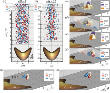
Pseudo-3-D reconstructed flow fields are shown in figure 5(a,b), from the two cross-plane measurement locations in the wake. Here, in order to more clearly identify structures with the swirling strength criterion, the planar, 3-component velocity fields were low-pass filtered (as before) via snapshot POD, retaining 67 % of total TKE by removing higher mode numbers. Upon being concatenated into pseudo-3-D fields, the in-plane grid resolution ( $\Delta y, \Delta z$) was then reduced through binning to match the out-of-plane resolution given by
 $\Delta x=U_c/f_s$. Isosurfaces of 3-D swirling strength show clear evidence of structures reminiscent of hairpin-shaped vortices populating the wake. In each case, instantaneous values of
 $\lambda _{ci}$ are normalized as
 \begin{equation} \lambda_{ci}^{*} = \lambda_{ci}\frac{\Delta x}{U_e} = \lambda_{ci}\frac{\Delta t U_c}{U_e} = \lambda_{ci}\frac{U_c}{f_s U_e}, \end{equation}
where  $f_s$ is the sampling frequency of the measurements (350 Hz herein). It is important to reiterate that the pseudo-3-D flow fields depicted here are not instantaneous volumetric realizations. Due to the non-stationarity of the flow and strong streamwise velocity gradients, as flow structures advect away from each respective measurement location, they are likely evolving and changing. This is also evidenced by the fact that the convection velocities found for the two measurement locations were slightly different (§ 3.1.3). As clarified above, these pseudo-3-D reconstructions using Taylor's hypothesis are only likely to be reflective of an instantaneous volumetric flow field within a 2
 $H$ streamwise extent around a given structure. Therefore, the volumetric flow fields depicted in figure 5(a,b) are best understood as a concatenated time series of flow structures that have advected through the measurement plane but are not simultaneously observed at one instant. The higher level of structural activity in reconstructions from
 $x/H=5$ compared with
 $x/H=6.5$, is likely due to the decreased turbulence at the downstream position as the wake grows and diffuses. As swirling strength is based on instantaneous velocity gradients and strongly influenced by small-scale activity, the flow therefore appears relatively cleaner at
 $x/H=6.5$.
(a,b) Isosurfaces of 3-D swirling strength from the isolated case showing reconstructions from time series of cross-plane stereo PIV measurements collected at  $x/H=5$ and 6, respectively; (c–f) conditionally averaged 3-D flow obtained in the measurement plane sampling events with consistent spanwise swirling (
 $\lambda _{ci,z}$); and (g,h) conditionally averaged 3-D flow obtained sampling on ejection events (
 $u<0$,
 $v>0$). Isosurface colours in (a,b) and (g,h) indicate the sign of streamwise swirling component (
 $\lambda _{ci,x}$), while isosurfaces themselves are extracted from
 $\lambda _{ci}^{*}=0.04$ for (a,b) and
 $\lambda _{ci}^{*}=0.03$ for (g,h). Isosurfaces in (c,d) plot conditionally averaged data from
 $x/H=5$ and isosurfaces in (e,f) plot data from
 $x/H=6.5$, both extracted using
 $\lambda _{ci}^{*}=0.026$. Isosurface values are chosen in each case to minimize visualization of noise and maintain consistency between data from the two measurement planes. Cross-sectional planes in (c–f) display in-plane velocity vectors overlaid with contours of
 $u$ and streamwise swirling,
 $\lambda _{ci,x}$.

With these limitations acknowledged, reconstructed volumetric velocity fields can still be used to compute conditionally averaged 3-D swirling strength isosurfaces (figure 5c–h) over the limited domain of 2 $H$ in the streamwise direction. Velocity field ensembles in figure 5(c–f) are conditioned on the identification of a spanwise swirling core along the centreline plane. As such, swirling strength fields were obtained by conditionally averaging around spanwise swirling cores identified anywhere in the
 $z/H=0$ plane within
 $y/H\in [0.75,1.5]$, with the origin set to the spanwise vortex core location. To aid visualization, resultant conditionally averaged fields were shifted such that the hairpin structure ‘head’ at the respective measurement plane's streamwise position was elevated to
 $y/H=1$ above the wall. Reconstructions from both the
 $x/H=5$ and
 $x/H=6.5$ cross-planes show similarity, where arched structures form with ‘legs’ that trail along in the streamwise direction, similar in spirit to a hairpin-like vortex. In-plane vector fields from x–y and y–z planes, overlaid with
 $u$ and streamwise swirling,
 $\lambda _{ci,x}$, highlight the ejection of low-momentum fluid underneath the head and between the legs, again consistent with that of a hairpin-like vortex.
Additional conditionally averaged flow fields were also generated by sampling on the occurrence of a  $Q_2$ ejection event (i.e.
 $u<0, v>0$). This approach yields very similar results, with isosurfaces of swirling strength, coloured by streamwise swirling strength, plotted in figure 5(g,h) revealing a spatial structure reminiscent of hairpin-like vortices. Here, the conditionally averaged structure has more clearly defined legs extending in the streamwise direction, as also indicated by the higher colour contour levels. This is likely because streamwise swirling motions directly induce
 $Q_2$ events, which are the conditioning criteria, whereas the previous approach (conditioning on a spanwise swirling motion) is not necessarily correlated with streamwise swirling motion. Nevertheless, this conditionally averaged 3-D flow structure, along with the time series of advecting flow structures (figure 5a,b), provide clear evidence that hairpin-like vortices populate the wake of the barchan dune, as was previously shown using LES by Wang & Anderson (Reference Wang and Anderson2018) and also inferred from low-frame-rate experiments by Bristow et al. (Reference Bristow, Blois, Best and Christensen2020).
3.1.3. Validating the choice of convection velocity
The convection velocities implemented herein were fine tuned by comparison with ‘ground truth’ velocity fields measured directly in the streamwise–wall-normal (x–y) centreline plane and reported by Bristow et al. (Reference Bristow, Blois, Best and Christensen2018). These measurements were made over the same physical models in a similar, but smaller scale, facility, for the same flow conditions such that the barchan was immersed at the same depth within the boundary layer. Following an approach similar to Dennis & Nickels (Reference Dennis and Nickels2008), comparisons were made of conditionally averaged flow fields from data directly measured in the x–y plane (with the same low-pass POD filter and binning applied as in the reconstructions, for consistency) to pseudo-x–y data reconstructed from the cross-plane measurements, using Taylor's hypothesis with several different uniformly applied convection velocities. The comparison (figure 6) is made for each of the two cross-plane measurement locations in terms of conditionally averaged spanwise swirling strength ( $\lambda _{ci,z}$) and
 $Q_2$ ‘ejection’ event probability. This approach is based on the premise that if hairpin vortices populate the wake region, both the reconstructed flow fields and the ground truth data should return features with similar spatial scales and spacing in the streamwise direction, at least near the streamwise position of the cross-plane measurement plane. A feature identification algorithm, similar to that used for tracking streamwise vortices, was used to (i) locate spanwise eddies in the x–y plane that are likely the heads of hairpin vortices, based on their typical signature in smooth-wall turbulent boundary layers (Adrian Reference Adrian2007), and (ii) conditionally average the flow field surrounding these identified motions. Thus, in figure 6, the conditionally averaged swirling strength fields of the ground truth and reconstructed data are compared, with the origins in each plot corresponding to the centre of the conditionally averaged spanwise swirling motions (hence the strong
 $\lambda _{ci,z}$ signal at the origin). The two cross-plane measurements are located at
 $x/H=5, 6.5$ and, therefore, within the ground truth dataset the conditional averaging algorithm searches only for hairpin heads located
 $\pm 0.5H$ of each respective measurement location.
Comparison between conditionally averaged ‘ground truth’ flow fields and conditionally averaged reconstructed flow fields in the wake of the isolated barchan. (a–d) swirling strength; (e–h) Q 2 event probabilities.

In the ground truth data, the swirling strength contours (figure 6a,b) exhibit secondary peaks aligned along  $\Delta y/H=0$. The spacing between these peaks represents the spatial distance between sequentially shed vortices in the ground truth data and consequently reflects their temporal distance in the reconstruction. As such, the comparison can be used to infer and validate the choice of convection velocity. In the ground truth data, this spacing is approximately
 $1H$ at both
 $x/H=5$ and
 $x/H=6.5$, judging primarily based on the closest (and likely most trustworthy) secondary peak at
 $\Delta x/H=1$. Adjusting the convection velocities for the cross-plane data to be
 $U_c=0.3U_e$ at
 $x/H=5$ and
 $U_c=0.35U_e$ at
 $x/H=6.5$ (approximately 30 % lower than the respective mean velocities), the spacings in secondary peaks of
 $\lambda _{ci,z}$ for the reconstructed fields agree well with the ground truth data. The spacings in the ground truth and reconstructed data are not perfectly periodic in either case, reflecting expected unsteadiness in this shedding behaviour that also introduces some uncertainty in identifying secondary peaks beyond
 $\Delta x/H\pm 1$. However, given that the application of Taylor's hypothesis is already an approximation, and the observation of secondary peaks at
 $\Delta x/H\pm 1$, the agreement over the reconstruction lengths used herein for individual conditional structures is deemed sufficient for the role that these reconstructions adopt in the present paper.
The spatial distribution of  $Q_2$ event probabilities (figure 6e–h) provides an additional metric for comparison between the ground truth and reconstructed data. It should be noted that the hairpin vortex-based identification algorithm for conditional averaging required the detection of not only a spanwise swirling motion, but also a trailing
 $Q_2$ event below and upstream of the spanwise swirling, as well as a shear layer in the instantaneous flow. Therefore, finding a very high probability of
 $Q_2$ events below and upstream of the origin, and a very low probability downstream and above the origin, is not surprising or meaningful in itself. However, what is revealing here is the agreement between the ground truth and reconstructed data in terms of the spatial extent of the contour levels in the streamwise direction, which for
 $P(Q_2)=0.5$ is approximately
 $1.5 - 2H$ in all four plots. This again provides further validation of the final convection velocities used herein for reconstruction.
If a larger or smaller convection velocity had been used for the reconstructions, the spacings between vortices and the spatial extent of  $Q_2$ probabilities in the reconstructed fields would merely be larger or smaller, respectively, with the same velocity fields stretched out in the streamwise dimension. It is important to note that the streamwise grid spacing of the reconstructed field is defined by the convection velocity, resulting in a coarser grid with increasing velocity. As such, in order to match the streamwise grid spacing, the in-plane grid density of the cross-plane measurements was downscaled through data binning.
An alternate approach, not used herein, would have been to use a spatially varying convection velocity, equal to the mean velocity in the cross-plane at the measurement location, for example (i.e.  $U_c(y,z) = \langle U(y,z) \rangle$). This approach is explored in Appendix A, where it is shown to have a similar effect as described previously, such that the resultant 3-D flow field is merely stretched out. In this case, the reconstructed flow fields would also be tilted in the streamwise direction with the mean shear. In addition, this approach produces an irregular grid in the streamwise direction that requires interpolation onto a regular grid of the reconstructed flow fields. As such, using a uniform convection velocity simplifies both analysis and interpretation (Dennis Reference Dennis2009; Hutchins et al. Reference Hutchins, Monty, Ganapathisubramani, Ng and Marusic2011), especially given that our interest is solely in qualitative aspects of the pseudo-3-D flow fields.
The approximate  $1H$ streamwise spacing of spanwise vortices (i.e. consistent with the heads of hairpin-like vortices) apparent in the planar conditional averages (figure 6a–d) is suggestive of a characteristic shedding frequency occurring in the wake. Converting the observed spatial wavenumber
 $\omega _x\approx 1/H$ into an equivalent temporal frequency,
 $f$, via
 $f=\omega _x U_c=U_c/H$, and using the incoming mean velocity at the height of the barchan as the characteristic velocity
 $U_0=U(x=-\infty ,y/H=1,z/H=0)$ and
 $H$ as the length scale, the Strouhal number associated with this vortex shedding is
 $St=fH/U_0=U_c/ U_0\approx 0.5$.
3.2. Spectral analysis
To investigate the presence of a spectral energy peak corresponding to the approximate  $1H$ streamwise structure spacing (equivalently
 $St\approx 0.5$), wavelet analysis is used. This approach involves a convolution between a ‘mother wavelet’ function
 $\psi (t)$ and the data signal (in this case
 $u(t)$), performed for varying temporal translation (
 $t'$) and dilatation (
 $s$) values to yield complex wavelet coefficients
 \begin{equation} G(t,s) = \frac{1}{\sqrt{s}}\int_{-\infty}^{+\infty} u(t') \psi^{*} \left(\frac{t-t'}{s}\right) \textrm{{d}}t', \end{equation}
where  $*$ indicates a complex conjugate. Furthermore,
 $t'$ can be intuitively understood as localizing the wavelet function in time, while
 $s$ provides a temporal scale associated with the wavelet function, and the coefficient
 $1/\sqrt {s}$ is an energy normalizing factor across dilatation values. Herein, the complex Morlet wavelet function is used as
 \begin{equation} \psi(t) = \textrm{e}^{{-}t^{2}/2}\textrm{e}^{-\textrm{i}bt}, \end{equation}
where  $b=6$ is a non-dimensional frequency parameter of the complex Morlet. Applying the convolution theorem to (3.2), wavelet coefficients
 $G(t,s)$ can efficiently be computed as
 \begin{equation} G(t,s) = \sqrt{s} \mathcal{F}^{{-}1}[\hat{\psi}^{*}(s\omega) \hat{u}(\omega)], \end{equation}
where
 $$\begin{gather} \hat{\psi}(\omega) = \mathcal{F}[\psi(t)] \end{gather}$$
 $$\begin{gather}\hat{u}(\omega) = \mathcal{F}[u(t)] \end{gather}$$
and  $\mathcal {F}$ and
 $\mathcal {F}^{-1}$ are the Fourier and inverse Fourier transforms, respectively. Using the conversion into frequency space for the wavelet coefficients via
 $f={b}/{2{\rm \pi} s}$, the instantaneous spectral energy can be calculated as
 \begin{equation} fE_{uu}(t,f)=f|G(t,f)|^{2}. \end{equation}
In figure 7(a,b), the premultiplied wavelet power spectra of  $u(t)$ and spanwise swirling strength
 $\lambda _{ci,z}(t)$, respectively, are plotted for a portion of the time series. These time series come from a grid point located at
 $(y,z)/H=(1,0)$ in the
 $x/H=5$ measurement plane. Figure 7(c) displays the integration of these two plots over the full time series to yield spectral energy as a function of frequency alone. These profiles, which are equivalent to the spectral energy distribution obtained via the relatively simpler Fourier transform of the times series, are normalized by their respective maxima to a scale of
 $[0,1]$ for comparison. Note that direct measurements of time-resolved
 $\lambda _{ci,z}$ realizations were not available in the present experiments, given the cross-plane orientation of the measurement domain wherein only streamwise swirling,
 $\lambda _{ci,x}$, is directly measured. Instead, the calculation of
 $\lambda _{ci,z}$ (as the imaginary component of the complex eigenvalue of
 $\partial U_i/\partial x_j$) at each time step involves the directly measured gradient
 $\partial U/\partial y$ and the time-local reconstructed gradient
 $\partial V/\partial x$ wherein
 $\partial /\partial x=-U_c\partial /\partial t$. This time-derivative calculation is performed using a central-difference approach with consecutive velocity fields acquired with a time difference of
 $\Delta t=2.86\ \mathrm {ms}= 0.09H/U_c$, where
 $U_c=0.3U_e$. This application of Taylor's hypothesis for local time derivatives is most accurate as it involves no significant evolution of the flow that might introduce unwanted error over longer time scales. The spectral energy distribution for
 $\lambda _{ci,z}(t)$ reflects the expected
 $St\approx 0.5$ based on the previous approximations, in support of the chosen convection velocity. The pre-multiplied global wavelet power spectrum of streamwise velocity fluctuations,
 $f\langle E_{uu} \rangle$, however, shows evidence of a much lower spectral peak corresponding to
 $St\approx 0.1$ (figure 7).
(a,b) Examples of pre-multiplied wavelet power spectra of (a)  $u$ and (b)
 $\lambda _{ci,z}$ from a grid point near
 $(y/H,z/H)= [1,0]$ in the measurement plane at
 $x/H=5$ for the isolated case; (c) global wavelet power spectra of
 $u$,
 $\lambda _{ci,z}$ and
 $\varPhi '_{\lambda _{ci,z}}$, normalized by respective maxima for visual comparison of frequencies associated with peaks. Solid lines indicate data from grid point near
 $(y/H,z/H)= [1,0]$ in measurement plane at
 $x/H=5$ and dashed lines from
 $x/H=6.5$. Horizontal dashed lines in (b) and thin vertical dashed lines in (c) indicate frequency band integrated over for
 $\varPhi '_{\lambda _{ci,z}}$.

The dynamics of large-scale structures in the flow is reflected in  $fE_{uu}$, the spectrum of which in the outer region is typically used to identify the imprint of LSM (e.g. Kim & Adrian Reference Kim and Adrian1999; Hutchins & Marusic Reference Hutchins and Marusic2007b). On the other hand,
 $fE_{\lambda _{ci,z} \lambda _{ci,z}}(t,f)$ displays a comparatively smaller scale associated with individual vortices, which is not entirely surprising given that swirling strength tends to emphasize smaller-scale activity due to the velocity gradients on which it is based. The question remains, however, as to whether there is a structural link between the two signals. To investigate this, we can leverage the strength of wavelet analysis wherein temporal information is retained, in order to uncover underlying periodicity in
 $fE_{\lambda _{ci,z} \lambda _{ci,z}}(t,f)$ itself. To that end, the bandpass filtered instantaneous spectral energy of
 $\lambda _{ci,z}$ is calculated as
 \begin{equation} \varPhi_{\lambda_{ci,z}}(t) = \left[ \int_{St=0.34}^{St=0.52} fE_{\lambda_{ci,z} \lambda_{ci,z}}\,\mathrm{d}\log_{10}(\,f) \right]^{1/2}, \end{equation}
where the range of integration  $0.34\leqslant St \leqslant 0.52$ corresponds to the dashed lines in figure 7(b,c) (i.e. the peak spectral energy band of
 $\lambda _{ci,z}$). After removing the mean, the fluctuating instantaneous energy,
 $\varPhi '_{\lambda _{ci,z}}(t)$, can be treated as a new time series upon which one can perform a global wavelet analysis (i.e. standard wavelet analysis followed by averaging over all time) to yield the third curve in figure 7(c). A significant overlap of this profile with
 $fE_{uu}$ suggests that the vortex shedding indicated by
 $\lambda _{ci,z}$, and the streamwise wavelength of
 ${\approx }1H$, is in fact superimposed upon a lower-order ‘pulsation’ in the wake that dominates the large-scale energy production captured by
 $fE_{uu}$. In other words, there are two dominant frequencies in the wake, with the higher frequency being manifested as the instantaneously observed hairpin-like vortices and the lower frequency indicating an episodic (i.e. discontinuous) nature to the vortex shedding events such that the hairpin-like vortices are shed in groups or ‘packets’.
This analysis, however, does not yet reveal a direct correlation between these two dominant frequencies. An appropriate measure of the extent to which the individual vortices (i.e.  $\lambda _{ci,z}$) are correlated with low-order, large-scale flow motions (reflected by the spectra of
 $u$) can be obtained via amplitude modulation analysis. Amplitude modulation herein generally refers to the interaction between two turbulent signals involving a significant scale separation, wherein the amplitude of the fluctuations in the small-scale quantity is either excited or attenuated by the large scale. By calculating normalized modulation coefficients, it is possible to quantify the extent to which the two signals are thus correlated, as well as any spatio-temporal phase difference. Following the approach of Baars et al. (Reference Baars, Talluru, Hutchins and Marusic2015) and Pathikonda & Christensen (Reference Pathikonda and Christensen2017), amplitude modulation coefficients,
 $R^{a}$, are herein calculated using low-pass filtered (instead of bandpass filtered, as before) fluctuating instantaneous energy of a small-scale signal,
 $\varPhi '_{sL}(t)$, and low-pass filtered large-scale signal,
 $u_L$ (where subscript
 $L$ indicates the low-pass filter). The frequency cutoff for low-pass filtering,
 $\,f_{{cut}}$, is chosen here via
 $St=0.2=\,f_{{cut}}H/U_0$ based on the crossing point between the spectral energy distributions of
 $u$ and
 $\lambda _{ci,z}$ in figure 7(c). The normalized modulation coefficients can then be calculated as
 \begin{equation} R_u^{a}(\Delta y,\Delta z,\Delta t) = \frac{\langle u_L(y_{ref}+\Delta y,z_{ref}+\Delta z,t-\Delta t) \varPhi'_{sL}(y_{ref},z_{ref},t) \rangle}{ \sqrt{ \langle u^{2}_L \rangle} \sqrt{ \langle \varPhi'^{2}_{sL} \rangle} }. \end{equation}
Using the convention above, positive  $\Delta t$ indicates a leading of the large-scale structures. In the study of near-wall turbulence modulation by outer large scales, the position of the large-scale signal is usually kept fixed while traversing the small-scale signal. Here, however, it should be noted that the small-scale signal,
 $\varPhi '_{sL}$ is held fixed while the large-scale
 $u_L$ is traversed. This is done such that if all three velocity components
 $u$,
 $v$ and
 $w$, are used in turn as the large-scale signal, a volumetric flow field can be constructed using the modulation coefficients. Similar to a linear stochastic estimation (Adrian Reference Adrian1994), this can be understood as the conditionally averaged flow field associated with a peak in the instantaneous spectral energy of the small-scale signal. Thus, if we take
 $\lambda _{ci,z}$ as a proxy for the shedding of the hairpin-like vortices observed in § 3.1.2, these amplitude modulation coefficients will reflect the approximate 3-D structure of the large-scale flow field associated with vortex shedding events.
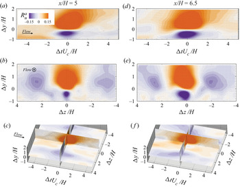
Figure 8(a,d) shows that a shear layer exists along  $\Delta y/H=0$ within approximately
 $\Delta tU_c/H\in \pm 1.5$, with a large, high-streamwise momentum region overlying a low-streamwise momentum region. This is expected to a certain degree, as the vortices would be shed via Kelvin–Helmholtz instabilities in the shear layer of the wake, and the hairpin-like vortices themselves should be associated with ejection of low-momentum fluid beneath the hairpin ‘head’, which has a clockwise swirling direction in the x–y plane. The cross-stream planes in figure 8(b,e) are more surprising, however, and by the same token are more informative about the origin of the large-scale structure correlated with the vortex shedding events. Two large-scale low-momentum (i.e. anticorrelation) regions flank either side of the central high-momentum region, with a spacing of roughly
 $2.5H$, bearing a strong similarity to the anticorrelation peaks observed in autocorrelations of
 $u$ in turbulent boundary layers. This structure in the outer region of the flow is typically indicative of LSMs whose streamwise wavelength is
 $O(\delta )$, and with a spanwise spacing similar to those observed here (
 $\delta /H\approx 5.5$). The streamwise extent of these low-momentum regions is shown in figure 8(c,f), where an additional low-momentum region is found to begin trailing the central high-momentum region for the measurements from
 $x/H=6.5$.
Amplitude modulation coefficients from measurements at (a–c)  $x/H=5$ and (d–f)
 $x/H=6.5$, all at (
 $y_{ref}$,
 $z_{ref})/H = (1,0)$ in wake of the isolated barchan, plotted as a volumetric velocity field, where colours denote the modulation coefficient associated with
 $u$. (a,d) Plot the slice of the flow field along
 $\Delta z/H=0$, (b,e) along
 $\Delta tU_c/H=0$ and (c,f) plot the previous two slices along with the slice at
 $\Delta y/H=0$.

While the correlation values,  $R^{a}$, are relatively low, these features of the spatial structure suggest that the LSMs present in the incoming turbulent boundary layer are responsible for modulating the shedding activity in the barchan wake. It can be hypothesized that passage of a high-momentum region, topographically forced over the top of the barchan, excites the shear layer separating from the crest (i.e. increasing
 $\partial U/\partial y$) causing roll-up of several vortices via the Kelvin–Helmholtz instability, and which then form into hairpin-like structures shed as organized packets. This interpretation explains the previously identified low frequency ‘episodic’ nature of the shedding activity. While causative conclusions are tenuous from correlations such as this, these results suggest that the overlying boundary-layer structure directly influences the shedding activity in the wake, and not the other way around, due to the significantly larger scales in the unperturbed boundary layer. Thus, it is likely that the frequency of vortex shedding in the barchan wake is modulated by that of the lower-order periodicity in the turbulent boundary layer due to alternating passage of high- and low- momentum LSMs.
To further substantiate this interpretation that the positive and negative correlations in the outer region of the flow are associated with the passage of LSMs in the overlying boundary layer, the same analysis was applied to datasets collected upstream of the isolated barchan, in a relatively unperturbed region of the flow, as well as in the wake of the smaller barchan in one of the collision cases (figure 9). For simplicity, the convection velocity for these datasets, required to generate reconstructed fields with which to extract a time series of spanwise swirling strength, was chosen to be identical to that of the isolated barchan at  $x/H=6.5$. The position of the measurement plane in the wake of the upstream barchan in collision B is also
 $6.5h$ downstream of its crest, where
 $h$ is the height of the smaller upstream barchan. Here, the focus is primarily on the spanwise and wall-normal dimensions of the outer structures rather than on comparing streamwise dimensions of the large scales from different planes, which would be entirely dependent on Taylor's hypothesis. Instead, Taylor's hypothesis is only used to calculate the local streamwise velocity gradients, and thus instantaneous spanwise swirling strength, from adjacent time steps at a given grid point. Spanwise swirling strength is then cast as a time series (i.e. reversing the application Taylor's hypothesis), in order to calculate modulation coefficients.
Amplitude modulation coefficients from (a) measurements in the relatively unperturbed region upstream of the isolated barchan at a reference location of  $(x_{ref}, y_{ref}, z_{ref})/H = (-2.5,1,-4)$ and (b) measurements in the wake of the smaller upstream barchan at a reference location of
 $(x_{ref}, y_{ref}, z_{ref})/H = (-2.5,0.5,-1.75)$. Coefficients are plotted as a velocity field, where colours are the modulation coefficient associated with
 $u$, taken from
 $\Delta tU_c/H=0$, and vector components are
 $R_v^{a}$ and
 $R_w^{a}$.

The ‘unperturbed’ dataset is taken from a streamwise position aligned with the toe of the isolated barchan ( $x/H=-2.5$), and the reference point for the calculation of the modulation coefficients is taken from the same height as that used in the wake of the barchan (
 $y/H=1$), but far off to the side and away from the barchan model as much as possible (
 $z/H=-4$) to avoid any topographical influence. These results (figure 9a–c) show a strong similarity to the results from the wake of the barchan, indicating that the large-scale structure found in the modulation coefficients (i.e. the flanking outer anticorrelation regions) comes from the incoming turbulent boundary layer, and is not a structure produced by the barchan itself. Hairpin-like vortices formed in smooth-wall turbulent boundary layers are known to be associated with LSMs (Adrian Reference Adrian2007), and therefore the similarity with the modulation coefficients in the wake of the isolated barchan supports the notion that those hairpin-like vortices formed by the barchan itself are also modulated by the LSMs in the overlying boundary layer, despite their formative mechanisms being distinct. It should be noted that the data plotted in figure 9(a) only contain positive
 $\Delta z$ values because the reference point is located at the spanwise edge of the measurement plane.
In further confirmation of this hypothesis, the results from the wake of the smaller, upstream barchan in collision case B (see figures 1c and 9b) show that the spatial extent of these outer region modulation coefficients does not scale with the size of the barchan, but rather with the thickness of the incoming boundary layer ( $\delta$). The upstream barchan in the collision cases is half as tall as the isolated barchan, and yet the approximate spacing between positive and negative modulation coefficients in the outer region is similar to the results from the wake of the isolated barchan.
3.3. Impulses of turbulent events
Having established this understanding of the dynamics and organization of turbulence in the barchan wake, attention is now given to the implications of these results for sediment transport and the morphodynamics of barchan dunes. In order to estimate the potential for sediment mobilization by the turbulent wake generated by a barchan dune, turbulent events can be accounted for independently in terms of the ‘impulses’ associated with contributions to the mean Reynolds shear stress,  $\langle -uv \rangle$. It is important to note again that these experiments involve smooth, rigid dune models immersed in flow without any sediment loading nor sediment transport occurring in the flume. Instead, this analysis is aimed at inferring where one might expect increased or decreased transport due to turbulence if the dunes and underlying bed were composed of an erodible substrate.
The impulse,  $J$, is herein defined as the integral of the Reynolds shear stress magnitude,
 $|uv|$, over the duration of a conditionally sampled event. These ‘events’ are defined according to canonical quadrant decomposition of
 $-uv$ based on the sign of
 $u$ and
 $v$ (Wallace Reference Wallace2016). Positive contributions to
 $\langle -uv \rangle$ are given by
 $Q_2$ ‘ejection’ events (
 $u<0, v>0$) and
 $Q_4$ ‘sweep’ events (
 $u>0, v<0$), which are associated with either low-momentum fluid being ejected away from the wall, or high-momentum fluid being swept down toward the wall, respectively. Negative contributions to
 $\langle -uv \rangle$ are given by
 $Q_1$ ‘outward interaction’ events (
 $u>0, v>0$) and
 $Q_3$ ‘inward interaction’ events (
 $u<0, v<0$).
By decomposing the Reynolds shear stress signal (measured at each grid point in the cross-plane) in this manner, the impulse of each quadrant can be calculated at each y–z location as
 \begin{equation} J_Q(y,z) = \frac{1}{N}\sum_{k=1}^{N} \left[ \int_{A_{Q,k}}^{B_{Q,k}}, |u(y,z,t)v(y,z,t)|\,\textrm{{d}}t\right] \end{equation}
where  $Q$ is the quadrant number,
 $k$ is the event number,
 $N$ is the total number of events registered and
 $A$ and
 $B$ are the beginning and end of an event, respectively. It is important to note here that
 $A$ and
 $B$ are not conditioned on a given threshold of
 $uv$, as is often done for quadrant analysis, such that low-magnitude
 $uv$ events with a longer duration are not overlooked. Moreover, the results herein are presented for all events that are registered in at least two time steps, but no other additional filtering is applied. The effects of filtering out relatively short duration events (events registered only for a few time steps), and which might be construed as noise, are demonstrated in Appendix B, and shown to be negligible. Using a characteristic duration,
 $H/U_c$, and magnitude,
 $u_{\tau }^{2}$,
 $J_Q$ can be normalized as
 \begin{equation} J_Q^{*}=\frac{J_Q}{J_c}=\frac{J_QU_c}{Hu_{\tau}^{2}}. \end{equation}
Note that in the following figures, small regions are masked out in white due to lower quality data resulting from imaging the flow directly through a sharp interface on the surface of the barchan model. Such challenges are attributable to finite RIM imperfections, the effects of which are amplified when imaging through a solid–fluid interface at a high incidence angle, and for higher-order flow statistics. Similar masking is absent in other plots, either due to their location or from the downscaling of the vector fields through data binning involved in pseudo-3-D reconstructions.
Figure 10(a–d) illustrates the spatial distribution of  $J_Q^{*}$ for each quadrant from the measurement plane at
 $x/H=5$. These results show that the turbulent impulse of an average
 $Q_2$ or
 $Q_4$ event here is significantly stronger than the impulse of an average
 $Q_1$ or
 $Q_3$ event, suggesting that
 $Q_1$ and
 $Q_3$ events are unlikely to be responsible for a significant amount of sediment transport. In order to reveal the relative contribution of
 $Q_2$ and
 $Q_4$ events and identify the distinct spatial regions of the wake where each of them is statistically dominant, figure 10(e) presents the difference between their respective impulses,
 $\Delta J^{*}=J_2^{*}-J_4^{*}$. In particular, near the wall and close to the barchan centreline,
 $Q_4$ events generate stronger average impulses, while further out in the span, for
 $|z/H|>1$, average
 $Q_2$ events generate a stronger impulse. Farther away from the wall, around
 $y/H=1$,
 $Q_2$ events clearly produce the strongest impulses.
(a–d) Average impulses from each of the four quadrant events, as indicated. (e) Disparity between  $Q_2$ and
 $Q_4$ event distributions. Data taken from
 $x/H=5$ for the isolated case, plotted with streamwise flow into page.

Examining impulse in terms of its components, duration and stress enables further insight into the dynamics of flow that gives rise to this spatial structure of mean impulse. Given that  $Q_1$ and
 $Q_3$ events appear negligible in terms of impulse, only the results for
 $Q_2$ and
 $Q_4$ will be considered hereafter. Figure 11(a–d) shows spatial distributions of normalized duration,
 $T_Q^{*}$, and stress,
 $S_Q^{*}$, respectively, which are defined as
 \begin{equation} T_Q^{*}=\frac{U_c}{H}\frac{1}{N}\sum_{k=1}^{N}\left( B_{Q,k} - A_{Q,k} \right) \end{equation}
and
 \begin{equation} S_Q^{*} = \frac{1}{u_{\tau}^{2}}\frac{1}{N}\sum_{k=1}^{N} J_{Q,k}(B_{Q,k} - A_{Q,k}). \end{equation}
As the product of the integral  $J_{Q,k}$ and its domain, each
 $S_{Q,k}$ is therefore the average magnitude of the Reynolds shear stress over the duration of the corresponding event. Additionally, both
 $T_{Q,k}^{*}$ and
 $S_{Q,k}^{*}$ are averaged over all recorded events.
Spatial distributions of average (a,c)  $Q_2$ and (b,d)
 $Q_4$ events, in terms of (a,b) event duration (
 $T_Q^{*}$) and (c,d) event stress (
 $S_Q^{*}$). Data taken from
 $x/H=5$ for the isolated case, plotted with streamwise flow into page.

The spatial distributions of  $T_2^{*}$ and
 $T_4^{*}$ (figure 11a,b) show that both
 $Q_2$ and
 $Q_4$ events have increased average durations in a specific quasi-circular region whose centre is located close to the barchan centreline and below its maximum height (
 $z/H\in [-1,1]$,
 $y/H\in (0,1]$). This suggests that the increased magnitude of turbulent impulses in this particular region of the wake are not only due to the significantly increased intensity of the turbulent stresses (figure 11c,d), but also an increased temporal coherence. The contours of
 $T_4^{*}$ are relatively constant across the span of the entire FOV with the exception of the aforementioned central region. However, contours of
 $T_2^{*}$ are particularly concentrated near the wall at the barchan centreline.
Given that the average stress of an event,  $S_{Q,k}$, is merely the impulse divided by the duration, the spatial distributions of
 $S_2^{*}$ and
 $S_4^{*}$ should follow a similar spatial distribution to that of the impulses after factoring out duration. Thus,
 $S_2^{*}$ and
 $S_4^{*}$ contours resemble that of
 $J_2^{*}$ and
 $J_4^{*}$ (figure 11c,d), with some minor differences due to the higher
 $T_2^{*}$ and
 $T_4^{*}$ values close to the centreline, as noted above. The disparities between the durations and stresses for
 $Q_2$ and
 $Q_4$ events are highlighted in figure 12, which demonstrates the relatively greater durations, yet lower stresses, of
 $Q_2$ events within
 $z/H\in [-1,1]$,
 $y/H\in (0,1]$. These trends are then inverted in the area above this domain, where instead
 $Q_2$ events have relatively shorter duration but higher stresses.
Disparity between distributions of  $Q_2$ and
 $Q_4$ event (a) durations and (b) stresses. Data taken from
 $x/H=5$ for the isolated case, plotted with streamwise flow into page.

The differences between  $Q_2$ and
 $Q_4$ events are further examined in terms of the durations of events with the strongest impulses (figure 13), i.e. those events most capable of influencing instantaneous sediment movement. This conditioning procedure is expressed as
 $T_Q^{*}(y,z)|{J_Q^{*}(y,z)>J_t}$, where
 $J_t^{*}\approx 2.1$ is chosen as an impulse threshold equal to the largest mean impulse of any event within the FOV. In a similar trend to the unconditional statistics for
 $T^{*}$, the
 $Q_2$ events characterized by the highest impulses are found to have significantly longer durations than
 $Q_4$ events of comparable impulse within
 $z/H\in [-1,1]$,
 $y/H\in (0,1]$. These conditionally averaged statistics provide a clear distinction in terms of the dynamics of
 $Q_2$ and
 $Q_4$ events that are most capable of influencing instantaneous sediment transport. Within
 $z/H\in [-1,1]$,
 $y/H\in (0,1]$,
 $Q_2$ turbulent events that are likely to transfer a significant amount of energy to grains through high impulse, causing mobilization, are characterized by a relatively lower stress yet sustained over a longer duration. The inverse holds for
 $Q_4$, whose high impulse events are characterized by higher intensities over shorter durations.
The  $Q_2$ (a) and
 $Q_4$ (b) event duration and stress distributions, conditioned on corresponding impulses above threshold
 $J_t$. (c) Disparity between panels (a,b). Data taken from
 $x/H=5$, plotted with streamwise flow into page.

This organization of  $Q_2$ events with long duration agrees with the organization of hairpin-like vortices shed in the wake of the barchan. The neck and legs of such structures should mutually induce
 $Q_2$ events between them, as shown in figure 5(c–f). The temporal coherence of streamwise vortices associated with the legs should then correlate well with the durations of
 $Q_2$ events, which is indeed observed in figure 4. It can be seen therein that the durations of
 $Q_2$ events agree most closely with the durations of streamwise swirling motions, particularly those of
 $TU_c/H>1.5$, compared with the other quadrant events.
3.4. Conditionally averaged structure of a  $Q_{4}$ event

While the relationship between  $Q_2$ events and the shedding and organization of hairpin-like vortices in the barchan wake is clear, the statistical dominance of
 $Q_4$ impulses near the wall along the barchan centreline is not as readily explained by the instantaneous observations of hairpin-like vortices in the wake of the barchan dune. Given the prevalence of these vortices, and the
 $Q_2$ events they induce, it might be expected that
 $Q_2$ events should have greater impulse near the wall about the centreline, instead of
 $Q_4$ events.
In order to understand this seeming contradiction, further insight can be gained from investigating the conditionally averaged  $Q_4$ structure in a 3-D reconstruction of the flow. In § 3.1.2, it was highlighted that when the flow is conditioned on a
 $Q_2$ event, the resulting hairpin-like structure surrounds that
 $Q_2$ event. Similar features were also observable in the pseudo-instantaneous realizations (figure 5a,b). Thus, the flow dynamics and structure giving rise to, or at least correlated with, a
 $Q_2$ event can be understood to some extent. For
 $Q_4$ events (figure 14a,d), this becomes less clear. Swirling strength isosurfaces, conditionally averaged on
 $Q_4$ events, display a spanwise swirling core, but no accompanying legs trailing behind it. Instead, if anything, it is more of an inverted hairpin structure, with more compact legs protruding in front (Hong et al. Reference Hong, Katz, Meneveau and Schultz2012; Jodai & Elsinga Reference Jodai and Elsinga2016). These features are difficult to reconcile with the pseudo-instantaneous structures in figure 5(a,b) and would suggest that the
 $Q_4$ events are not directly associated with hairpin-like structures. While this is not surprising, it might be expected that a
 $Q_4$ event would always precede the passage of a hairpin, due to the prograde spanwise swirling motion induced by the head of the vortex. However, this does not appear to be the case and, although a spanwise swirling motion is found upstream of the
 $Q_4$ event, there is no clear indication that this is part of a coherent hairpin-like structure.
Conditionally averaged flow fields from the isolated case associated with (a,b,d,e)  $Q_4$ events and (c,f)
 $Q_2$ events. (a,d) Isosurfaces of swirling strength coloured by its spanwise swirling component (
 $\lambda _{ci,z}$) with in-plane vectors in the centreline x–y plane overlaid; (b,c,e,f) isosurfaces of
 $u$.

Instead, it is informative to inspect the isosurfaces of  $u$ in the flow field conditioned on a
 $Q_4$ event. Plotting these isosurfaces (figure 14b,e) shows that a large-scale high-momentum region (
 $u>0$) is associated with the
 $Q_4$ event. Moreover, this structure is flanked by two low-momentum regions (
 $u<0$). These structures extend quite far upstream and downstream of the
 $Q_4$ event, and also occupy a greater wall-normal distance above the wall, unlike the conditionally averaged
 $u$ isosurfaces associated with a
 $Q_2$ event, which are more compact in the streamwise direction (figure 14c,f). This is particularly evident in the measurements from
 $x/H=6.5$ where the structures also appear more coherent and extend into the outer region with an inclination away from the wall. Therefore, these results suggest that a more likely explanation for the dominance of
 $Q_4$ event impulses near the wall is that these sweeps of high-momentum fluid come directly from the outer region of flow in the overlying turbulent boundary layer. In other words, they are not directly linked to individual vortices shed by the barchan, and instead are associated with high-momentum LSMs as these structures advect over the barchan, into its wake, and impinge on the bed during flow reattachment events. In this manner, the sweep events in the wake can also be understood to be likely modulated by the large-scale structure of the incoming turbulent boundary layer.
3.5. Collisions
Having explored the dynamics and organization of turbulence structures in the wake of an isolated barchan, measurements taken from the region between two interacting barchans can shed light on how the wake of an upstream barchan dune (hereafter referred to as UBD) can influence the flow structure over a downstream barchan dune (hereafter referred to as DBD). First, the distribution of turbulent impulses associated with  $Q_2$ and
 $Q_4$ events in the interdune region are examined for all three collision cases (A, B and C). Figure 15 presents the differences in the average impulse associated with a
 $Q_2$ and a
 $Q_4$ event. A progression can be observed, from a strong similarity to the wake of the isolated barchan in the early stage of the collision (figure 15a), to a highly asymmetric distribution in the final stage, when the barchan dunes are in closest proximity (figure 15f). The panels on the left (figure 15a–c) all show data aligned with the toe of the DBD, while the panels on the right (figure 15d–f) show data overlying the stoss side of the DBD. As was discussed in greater detail by Bristow et al. (Reference Bristow, Blois, Best and Christensen2020), asymmetries in the turbulence statistics in the interdune region are driven by the lateral offset between the DBD and UBD. This asymmetry can be seen here to manifest itself as a skewed spatial distribution of impulses, where
 $Q_2$ has higher impulse (i.e. positive
 $\Delta J^{*}$) farther to the outside, away from the DBD. The impulses of
 $Q_4$ events remain dominant in the near-wall region, with only a minor spatial shift as the UBD wake veers off to the side (Wang et al. Reference Wang, Tang, Bristow, Blois, Christensen and Anderson2017; Bristow et al. Reference Bristow, Blois, Best and Christensen2018).
Impulse differences between  $Q_2$ and
 $Q_4$ events in the interdune region during collision cases A–C. Dashed lines in (b,d,f) indicate DBD stoss side topography transected by measurement plane.

The asymmetry in  $Q_2$ impulses observed herein can be understood as the imprint of hairpin-like vortices shed in the UBD wake that are altered by the proximity and offset alignment of the DBD, as was proposed by Bristow et al. (Reference Bristow, Blois, Best and Christensen2020). Evidence of this behaviour can be seen in pseudo-3-D reconstructions of flow in the interdune region (figure 16) at
 $x/H=-2.5$ for collision B, and
 $x/H=-1$ for collision C. These two measurement planes take data from a streamwise distance
 $6.5h$ downstream of the UBD crest, where
 $h$ is the UBD height, in each case. This is the same relative distance from the crest as was examined for the isolated barchan at its farthest downstream measurement position,
 $x/H=6.5$, and thus for simplicity the same convection velocity
 $U_c=0.35U_e$ was used. From the time series of pseudo-instantaneous structures, hairpin-like vortices can be observed in both cases that are quite similar to that observed in the wake of the isolated barchan. It should be noted that the application of Taylor's hypothesis here only involves a streamwise convection velocity (as before), despite the fact that there is a non-zero mean spanwise velocity throughout the bulk of the UBD wake. In other words, the vortices reconstructed in figure 16(a,b) would appear to advect directly through the DBD, while in reality these structures will also advect laterally to move around the DBD. For simplicity in these reconstructions, attempting to introduce any lateral advection is avoided, and therefore the topography of the DBD is not shown, only its planform projection.
Isosurfaces of 3-D swirling strength from collision cases B and C showing (a,b) reconstructions from time series, (c,d) flow reconstructions conditionally averaged on ejection events ( $u<0, v>0$). Isosurface colours indicate the sign of streamwise swirling component (
 $\lambda _{ci,x}^{*}$), while isosurfaces themselves are extracted from
 $\lambda _{ci}^{*}=0.03$ in (a,b) and
 $\lambda _{ci}^{*}=0.025$ in (c,d). Isosurfaces in (a,c) plot conditionally averaged data from
 $x/H=-2.5$ in collision case B and isosurfaces in (b,d) plot data from
 $x/H=-1$ in collision case C. Isosurface values are chosen in each case to minimize visualization of noise.

Despite this approximation, conditionally averaged flow fields are informative, particularly for directly comparing the measurements from the two collision cases. Conditionally averaging the flow field on the occurrence of a  $Q_2$ event yields the 3-D structures shown in figure 16(c,d). While the conditionally averaged interdune structure in collision B is relatively symmetric, resembling that observed in the wake of the isolated barchan when conditioned in the same manner (figure 5g,h), the structure from collision C is distinctly asymmetric, with its right leg extended over a greater streamwise extent. The structure shown here closely resembles the cartoon depiction postulated by Bristow et al. (Reference Bristow, Blois, Best and Christensen2020), resembling a ‘cane’ vortex. This confirms the notion that the strong asymmetry in the mean swirling strength presented by Bristow et al. (Reference Bristow, Blois, Best and Christensen2020) within the interdune region is, in fact, the imprint of distorted hairpin-like vortices that are altered due to interaction with the DBD.
The spanwise asymmetry of the structure means that the motions induced by its legs will be out of balance. Therefore, an ejection of low-momentum fluid in between the legs, which would otherwise be directed upward (i.e. without a preferential spanwise direction) in the case of a symmetric hairpin, will now be pushed primarily to the side where the leg is weaker or missing. Therefore, since the hairpin leg that is closest to the DBD is more coherent than the opposing leg in collision C, it can be expected that  $Q_2$ events should be more dominant on the far side of the wake (i.e. farther from the DBD). This proposition agrees with the results shown in figure 15(e,f), where the region of the flow where
 $Q_2$ event impulses are most dominant over
 $Q_4$ events is concentrated asymmetrically farther out in the span.
4. Discussion
4.1. Mechanism for hairpin-like vortices, $Q_{2}$ events, and $Q_{4}$ events in the wake of a barchan dune


A physical mechanism for the dynamics of turbulence in the wake of a barchan dune presented herein can be postulated as follows. When a high-speed (i.e.  $u>0$) LSM from the incoming turbulent boundary layer approaches a barchan dune, it is lifted up over the dune and into the wake. This high-speed LSM in turn forms the upper half of the shear layer that characterizes the wake region, where the flow has separated. As noted previously, the presence of this high-speed LSM excites the shear layer (as the velocity gradient across the layer will be greater than its average value), amplifying the instability, and resulting in the promotion of vortex roll-up and formation of hairpin-like vortices.
It can be hypothesized that the formation of hairpins in the shear layer drives a rapid mixing of the overlying high-speed flow brought by the LSM with the low-speed flow near the wall. In other words, the passing high-speed LSM has driven the flow around it to be locally more turbulent and effective at mixing. As the newly formed vortices mix the flow, the boundary between the low-speed flow near the wall and the overlying high-speed flow shifts closer to the wall, as momentum is diffused from the outer region downward. This process culminates in a strong  $Q_4$ event, as very high-speed flow (in a relative sense) has been brought from the outer region close to the wall. If the high-speed LSM is particularly elongated in the streamwise direction, then the duration of the
 $Q_4$ event felt near the wall will be correspondingly longer, and thus for a given magnitude of the fluctuation, will result in a greater turbulent impulse. Once the high-speed LSM has passed, the low-momentum region of the wake effectively begins to expand away from the wall again and the shear layer moves outward in what is likely a period of relative inactivity (in terms of vortex shedding), which explains the observed intermittency of the vortex shedding.
With all of this in mind, it is therefore not surprising that  $Q_4$ events, being associated with passing high-speed LSMs themselves, will have correspondingly greater turbulent impulses, in comparison with the
 $Q_2$ events, which are locally induced by individual vortices. Due to the blockage of the wall,
 $Q_2$ events are limited in how great a velocity differential (i.e. fluctuation) they can be associated with, at least close to the wall. A
 $Q_4$ event, on the other hand, can be associated with very strong fluctuations depending on how far from the wall the ‘sweep’ of high-speed fluid originated. From this perspective, despite the presence of hairpin-like vortices straddling the barchan centreline as the predominant structure formed in the wake,
 $Q_4$ events will still be more dominant close to the wall, due to their intensity, than the
 $Q_2$ events induced by these structures.
Farther away from the barchan centreline, however, this relative dominance of  $Q_4$ events over
 $Q_2$ events understandably changes. The velocity deficit is greatest near the centreline, and thus
 $Q_4$ events here have the greatest potential to possess very intense fluctuations. Away from the centreline,
 $Q_2$ events are able to become more dominant over
 $Q_4$ events. Indeed, it should be noted that while the vortices that induce the
 $Q_2$ events are, on average, centred at
 $z/H=0$, they are not stationary or fixed in space, as can be seen in the pseudo-instantaneous reconstructions (figure 5a,b), where vortices are not all perfectly aligned with the centreline.
4.2. Interaction of roughness elements with boundary-layer LSMs
If we consider flow associated with barchan dunes on the scale of the boundary layer itself, these bedforms can be considered as roughness elements protruding into the log layer of the overlying turbulent boundary layer. Studies of similarly scaled roughness elements are typically motivated by progress towards passive control of the turbulent boundary layer through modification of the near-wall flow (Tomkins Reference Tomkins2001; Jacobi & McKeon Reference Jacobi and McKeon2011; Ryan et al. Reference Ryan, Ortiz-Dueñas and Longmire2011; Zheng & Longmire Reference Zheng and Longmire2014; Pathikonda & Christensen Reference Pathikonda and Christensen2015; Tang et al. Reference Tang, Jiang, Zheng and Wu2016; Tan & Longmire Reference Tan and Longmire2017). Therefore, although the aspect ratios ( $H/W$) of barchan dunes are much lower than hemispheres and cylinders typically considered in such contexts, the insights gained from these prior studies remain relevant to how one should interpret the interaction of the barchan wake with the overlying turbulent boundary layer. Studying wall-mounted cylinders and hemispheres protruding into the boundary layer at
 $H/\delta \approx 0.15$, Tomkins (Reference Tomkins2001) showed that hemispheres produced more intense spanwise swirling motions associated with hairpin vortices, but was unable to extract a clear shedding frequency using autocorrelations of
 $u$ and
 $\lambda _{ci,z}$. Tomkins (Reference Tomkins2001) postulated that boundary-layer turbulence, within which the elements were immersed, disrupted this shedding process. This result does not contradict our findings herein, as we have shown that the LSMs in the boundary layer in fact modulate the vortex shedding, such that hairpin-like structures do not appear perfectly periodically, but in bursts of shedding events, followed by more quiescent periods of flow. This effect would inhibit clear periodicity being reflected in any autocorrelation analysis, and therefore the results presented herein provide a possible explanation as to why Tomkins (Reference Tomkins2001) did not find a clear shedding frequency. Ryan et al. (Reference Ryan, Ortiz-Dueñas and Longmire2011) showed that cylinders with height-to-diameter ratios of
 $H/D=1.5$ attenuate the premultiplied power spectral energy and root mean square of
 $u$ in the near-wall region, shifting the energy away from the wall. These effects were capped at the top of the log layer, however. Jacobi & McKeon (Reference Jacobi and McKeon2011), studying a short fetch of 2-D roughness elements, showed that the near-wall impact of the roughness elements was not continuous across the spectrum, but selectively interacted with wavelengths in the boundary layer, suppressing the large scales near the wall. Pathikonda & Christensen (Reference Pathikonda and Christensen2015) showed results similar to both Ryan et al. (Reference Ryan, Ortiz-Dueñas and Longmire2011) and Jacobi & McKeon (Reference Jacobi and McKeon2011) using hot-wire anemometry in the wakes of slightly higher aspect ratio cylinders, up to
 $H/D=2.55$. They noted, however, that the three-dimensionality of the cylinders aided more rapid recovery of the boundary-layer spectral energy content than for 2-D roughness of equivalent height. Zheng & Longmire (Reference Zheng and Longmire2014) further developed these ideas concerning the interaction of roughness elements with the large-scale structure in a turbulent boundary layer by studying the perturbation and recovery of hairpin vortex packets behind spanwise arrays of cylinders protruding into the log layer. They found that hairpin packets from the incoming boundary layer recovered over relatively short distances of 2
 $\delta$ downstream, and therefore suggested a top-down mechanism of recovery, wherein the packets were not destroyed by the cylinder arrays. Instead, the significant wall-normal extent of the packets meant that they retained some of their structure and propagated gradually downwards to the wall. This result agrees with the interpretation of the results herein, which rely on the assumption that LSMs in the boundary layer are not completely broken apart by the presence of the barchan, but are instead lifted above the barchan through an even more gentle topographic forcing than would be encountered in an interaction with a cylinder. The concept of top-down recovery was shown in the subsequent study of Tan & Longmire (Reference Tan and Longmire2017) to be exclusive to roughness elements that do not occupy the entire boundary-layer thickness. Comparing cylinders with
 $H/\delta =0.2$ and
 $H/\delta =1$, Tan & Longmire (Reference Tan and Longmire2017) found that the taller cylinder featured a bottom-up recovery of vortex packets in its wake, such that the cylinder had completely disrupted the passing LSMs in contrast to the log-layer cylinder. Tang et al. (Reference Tang, Jiang, Zheng and Wu2016) showed that amplitude modulation of the small scales by the large scales observed in smooth-wall boundary layers was robust to the presence of a cylindrical roughness element. Their cylinder had a relatively low aspect ratio of
 $H/D=0.58$, remaining immersed in the log layer, and while changes to the modulation of bursting events were observed, the overall behaviour was similar to that found in smooth-wall boundary layers. This provides further support to the notion that the modulating LSMs are not wholly destroyed by such roughness elements, as was noted in the studies cited above.
These observations from past studies support, in general, the conclusion that amplitude modulation by the large scales plays a significant role in the vortex shedding process in the wake of the barchan dune, through the excitation of the shear layer as high-momentum LSMs pass over the barchan and into its wake and remain intact. Moreover, it is also reasonable to expect that such instantaneous turbulent dynamics are imprinted on the statistics of turbulent impulses by facilitating more intense  $Q_4$ sweep events near the wall along the centreline, as discussed in § 3.4.
4.3. Implications for barchan morphodynamics
The interaction between the turbulent boundary layer and the wake of the barchan dune suggests that the flow environment associated with natural barchans may play a role in the precise dynamics of their long-range interactions during collisions between barchans. For instance, although a mobile barchan dune may be immersed in the log layer of a flume channel, the LSMs in the boundary layer or channel flow would be affected by the Re of the flow. If the Re is not large enough, the modulating effect of LSMs may not be as significant in influencing flow in the barchan wake, particularly for the sweep events. For an aeolian barchan, the spatial structure and modulating effects of LSMs are altered in the atmospheric surface layer by buoyancy effects under convective instability (Chauhan et al. Reference Chauhan, Hutchins, Monty and Marusic2013; Salesky & Anderson Reference Salesky and Anderson2018). Thus, for the same wind strength, the dynamics of vortex shedding in the barchan wake could be altered by convective instability. Such changes in boundary layer turbulence could, therefore, influence wake-dominated barchan interactions through the capacity of an upstream barchan to enhance transport over the downstream barchan (Assis & Franklin Reference Assis and Franklin2020).
While the precise link between hairpin-like vortices and sediment transport, whether as bedload, saltation or suspension, remains to be fully elucidated, many studies have shown that instantaneous turbulent events, identified as sweeps, ejections, and inner–outer interactions, play key roles in sediment transport and its intermittency and variability. Studies have shown that bedload transport is strongly correlated with  $Q_4$ sweeps (e.g. Williams & Kemp Reference Williams and Kemp1971; Grass Reference Grass1983; Best Reference Best1992; Nelson et al. Reference Nelson, Shreve, McLean and Drake1995), while
 $Q_2$ ejections are particularly important for sediment suspension (Jackson Reference Jackson1976; Leeder Reference Leeder1983; Amirshahi et al. Reference Amirshahi, Kwoll and Winter2018; Li et al. Reference Li, Balachandar, Lee and Bai2019). Moreover, aeolian ‘streamers’, which are a primary manifestation of saltation transport (Baas & Sherman Reference Baas and Sherman2005) are thought to be associated with
 $Q_4$ sweeps and are initiated trailing the passage of LSMs (Wang et al. Reference Wang, Feng, Zheng and Sung2019). Based on the results herein, the wake of a barchan dune is characterized by shedding of packets of hairpin-like vortices, which primarily induce
 $Q_2$ ejections, followed by a strong reattachment event as the aloft high-speed LSM reaches the bed, thus inducing
 $Q_4$ sweeps. The cycling between these two states could result in sediment being mobilized as bedload, and initiation of saltation by the reattachment event could further aid entrainment into suspension by the passage of the next set of hairpin-like vortices. Although the present study does not involve mobile sediment, and therefore these inferences are speculative, it does support past work that has suggested the important links between
 $Q_2$ and
 $Q_4$ events generated over bedforms and their role in bedload and suspended load transport (Bennett & Best Reference Bennett and Best1995, Reference Bennett and Best1996; Best Reference Best2005a,Reference Bestb).
For the barchan collision scenarios examined herein, results did not indicate a fundamental change in the organization of the wake flow or its interaction with the overlying boundary layer, apart from a strong asymmetry in the final stages of the laterally offset collision. It is noteworthy, however, that the asymmetric hairpin-like vortices found via conditional averaging in the interdune region are significantly more coherent in the streamwise direction during the final collision stage (figure 16d). This additional coherence would likely increase the potential for sustaining or enhancing sediment transport.
A similar elongated streamwise vortex to that elucidated herein was shown in the interdune region for laterally offset barchan collisions in the flow simulations of Wang & Anderson (Reference Wang and Anderson2018, Reference Wang and Anderson2019). However, the mechanism postulated for its formation, mainly related to flow channelling effects, is different from the observations reported herein, as well as the statistics of streamwise vortices shown by Bristow et al. (Reference Bristow, Blois, Best and Christensen2020). It is apparent that the long streamwise structure in the interdune region is a component of a highly asymmetric hairpin-like structure that still retains a spanwise swirling motion as the head (figure 16d). The reason for the consistent asymmetry in the legs of the hairpin, and thus the sustained streamwise swirling motion, seems to be the interaction of this hairpin shed by the upstream barchan with the downstream barchan. As was shown by Bristow et al. (Reference Bristow, Blois, Best and Christensen2020), the stoss side topography of a barchan organizes the flow into counter-rotating streamwise swirling motions on either side of the barchan. This topographic forcing thus interacts with the nearest leg of the hairpin-like vortex that is shed, amplifying it and sustaining its asymmetry. Regardless of the precise mechanism, however, it has been shown by Wang & Anderson (Reference Wang and Anderson2019) that these streamwise vortices formed in offset collisions are prevalent in dune fields and, on the scale of the boundary layer itself, are an important part of the ‘dune field sublayer’ flow structure.
Lastly, although the barchan dune collision studied herein only considered one size of upstream barchan, based on our understanding of the flow physics some implications can be hypothesized concerning collisions between barchans of various sizes, as investigated by Endo et al. (Reference Endo, Taniguchi and Katsuki2004) and Assis & Franklin (Reference Assis and Franklin2020). These experimental investigations of subaqueous barchans showed that the ratio of the sizes of the two bedforms exerts a first-order control on the resultant morphodynamics, where larger upstream barchans have more potential to erode the downstream dune compared with smaller dunes. In the present study, hairpin-like vortices shed in the wake of the barchan are found to typically be aligned with the height of the dune, and can thus be expected to scale approximately with dune height. This contention is reflected by the fact that vortices shed by the upstream barchan in the current study are generally smaller in scale than those shed by the larger, isolated barchan. Thus, the coherence of flow motions that are induced by these hairpin-like vortices can be inferred to scale roughly with the size of the barchan. Naturally, this has implications for sediment transport, which relies on flow impulse and coherence. However, perhaps more important is the disparity between the momentum deficit in the wake of the barchan and the momentum excess of LSMs that are lifted over the barchan and lie above the shear layer. This disparity directly impacts the intensity of  $Q_4$ sweep events. Larger barchan dunes will therefore be characterized by a larger momentum disparity, resulting in a greater potential for intense sweeps and enhanced sediment transport similar to that shown by Bacik et al. (Reference Bacik, Lovett, Colm-cille and Vriend2020).
5. Summary and conclusions
PIV measurements were made of flow over solid barchan dune models immersed in a turbulent boundary layer, both for an isolated barchan as well as for several stages of interaction of laterally offset dunes. High-frame-rate measurements of the flow field in the spanwise–wall-normal (i.e. cross) plane enabled analysis of the time-resolved dynamics of turbulent flow in the wakes of the barchans, allowing reconstruction of pseudo-3-D flow fields and derivation of time-averaged statistics upon which such instantaneous features leave their imprint. From this analysis, four principal conclusions can be drawn.
First, the flow field in the wake of an isolated barchan dune is populated with hairpin-like vortices that are shed from the barchan dune. However, the manner in which these vortices are shed is not perfectly periodic, and is instead intermittent, and modulated by the passage of LSMs in the overlying boundary layer. The presence of the barchan dune does not completely break-up these LSMs, but rather lifts them over the barchan, and into the bedform wake, where, if the LSM is a high-momentum structure, they excite the aloft shear layer during their passage. This interaction promotes vortex roll-up via amplification of the Kelvin–Helmholtz instability and shedding of vortices. The shedding activity is attenuated with the departure of the high-momentum LSM, culminating in a reattachment event. The characteristics of these interactions have generic implications for how one understands the interaction of roughness elements that protrude into the logarithmic region of turbulent boundary layers.
Second, the dynamics of these coherent structures in the barchan wake leaves its imprint on the average impulses of Reynolds shear stress contributions (i.e. sweeps, ejections and inner–outer interactions). Sweeps and ejections have the strongest turbulent impulses on average, yet are distinct in their characteristics. Sweep events, which have stronger impulses near the wall along the barchan centreline, as compared with ejection events, are shown to be associated with relatively short, but intense, turbulent fluctuations. Ejection events, on the other hand, dominate the rest of the wake region in terms of impulse, but are characterized by relatively longer durations of lower intensity, as compared with sweeps in the same region. These ejections are associated with the hairpin-like vortices, while intense sweeps most likely occur with the LSM-induced reattachment events.
Third, collisions between barchan dunes involve similar flow structures controlling the dynamics of turbulence in the interdune region. The flow in this region is modified, however, by the presence of the downstream barchan with a lateral offset, which induces an asymmetry in the hairpin structures shed by the upstream barchan as they advect downstream. The spatial distribution of where sweeps and ejections have their greatest impulse in a mean sense is thus somewhat asymmetric, but is shown to remain fundamentally unchanged.
Lastly, the results presented herein have implications for understanding how sediment transport over and around a downstream barchan is altered by the presence of an upstream barchan. The turbulence is highly intermittent, yet also retains an underlying organization. Critically, the flow structures shed by the upstream barchan and the turbulent events in the wake are controlled in their scale and coherence by the size of the upstream barchan. Moreover, these results allow characterization of the likely mechanisms of sediment transport in the wake of a barchan dune, or on the stoss of a downstream dune during a collision or interaction. This characterization, and the intimate links between LSMs and near-bed turbulence, have implications not only for the dynamics of sediment transport associated with barchan dunes, but also a wide range of bedform interactions (Bennett & Best Reference Bennett and Best1995; Fernandez et al. Reference Fernandez, Best and López2006) as well as flow over rough-bed gravel beds (Roy et al. Reference Roy, Buffin-Belanger, Lamarre and Kirkbride2004).
Funding
This work was supported by the US National Science Foundation through collaborative grants CBET-1603211 (Notre Dame) and CBET-1604155 (Illinois).
Declaration of interests
The authors report no conflict of interest.
Appendix A. Varying convection velocity reconstructions
Pseudo-3-D reconstructions of flow structures, identified using the swirling strength criterion, are compared in figure 17, with the only difference between the panels being the use of a uniform convection velocity (figure 17a) and a spatially varying convection velocity (figure 17b). Both reconstructions are made using the same sample of cross-plane measurements, which are taken from the same set as plotted in figure 5(b) associated with the  $x/H=6.5$ plane. The structure visible in the centre of the flow field, and consistent with a hairpin-like vortex, in the uniform
 $U_c$ case is also identifiable in the spatially varying
 $U_c$ case. However, in the latter case this structure has been significantly elongated in the streamwise direction. Here, instead of the legs of the structure curving away from the wall to connect to the head, they are angled linearly away from the wall. Thus, in a qualitative sense, the same flow structures are identified, and their shape is not fundamentally changed by the choice of convection velocity, but rather they are simply distorted.
Comparison of isosurfaces of swirling strength reconstructed from the  $x/H=6.5$ measurement plane in the wake of the isolated barchan, using (a) uniform convection velocity,
 $U_c=0.35U_e$ and (b) spatially varying convection velocity equal to the local mean streamwise velocity,
 $U_c(y,z)=\langle U(y,z) \rangle$.

Appendix B. Event duration thresholding
The effects of filtering out short duration events from the turbulent events used to calculate the impulse statistics are demonstrated in figure 18. The left-hand panels (a,c,e) display the same data from figures 10(e) and 12 (i.e. without a minimum duration filter applied) except with a colour scale such that they are comparable to the right-hand panels, for which a minimum duration filter was applied. This ‘minimum duration’ was somewhat arbitrarily chosen to be four time steps ( $\Delta t = 1/f_s$) in order to remove any relatively short events that could be construed as noise in the data. The trends between the unfiltered and filtered data are quite similar, with the only difference being that the average magnitude of impulses, durations and stresses are larger for the thresholded data. This trend is to be expected, as short duration events will, in general, have weaker impulses and will contribute to reducing the average. The conclusions drawn regarding the spatial regions where
 $Q_2$ ejections have a relatively long duration, but lower stress, as compared with
 $Q_4$ sweeps, are therefore unchanged.
Differences between  $Q_2$ and
 $Q_4$ for average (a,b) impulse, (c,d) duration and (e,f) stress, comparing results obtained (a,c,e) without any thresholding, and (b,d,f) a minimum duration threshold of four measurement time steps applied. All data from
 $x/H=5$ for the isolated case.