I. INTRODUCTION
A digital transmitter used in wireless communication applications comprises several stages including a digital baseband, digital-to-analog converter (DAC), modulator, and power amplifier (PA). In general, a PA has a nonlinear gain, which is not desired. As a result, the transmitter often includes a baseband linearization method such as digital predistortion (DPD) [Reference Braithwaite and Luo1]. Unfortunately, the predistorted signal requires a wider bandwidth than the linear (original) signal to accommodate the compensation provided by the DPD. The Nyquist rate of the linear signal is not sufficient to represent the predistorted signal digitally without aliasing. In this paper, the sampling requirements for digitally predistorted signals used to compensate for nonlinear power amplifiers are investigated. In addition, the delay offset (spacing) between taps within memory-based DPD models is discussed.
Nonlinear amplification transforms the input signal into a linear component and several nonlinear components related to the polynomial order of the nonlinearity. The components created are referred to as modes of the PA. Sampling requirements for nonlinear modes have been discussed briefly in [Reference Braithwaite2]. Most DPD systems over-sample the digital domain reducing the practical impact of such problems. However, as signal bandwidths increase (e.g., to 100 MHz for LTE-Advanced) there becomes a greater need to understand the minimum sampling requirements for DPD.
The outline of the paper is as follows. Nonlinear representations of the PA response to band-limited signals are discussed in Section II. In Section III, an equivalent digital model of the PA response is formed by back projecting the RF nonlinearity to a sampled baseband. The sampling requirement for each nonlinear mode is determined as a function of the polynomial order. Examples are provided in Section IV to illustrate how the theory can be utilized in a DPD system. Section V provides recommendations and discusses future work.
II. REPRESENTATIONS OF PA NONLINEARITIES
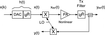
Consider a digital transmitter without predistortion, as shown in Fig. 1. An analog baseband signal x(t) is derived from a digital sequence of complex symbols x(k):
 $$x\lpar t\rpar =\sum\limits_k^{} {x\lpar k\rpar h\lpar t - kT\rpar }\comma \; \eqno\lpar 1\rpar$$
where T is the time interval between symbols and h(t) is an interpolation function that fills in between the discrete samples located at t = kT. In a typical digital communication system the interpolation function is the impulse response of the channel filter.
Digital transmitter with an observation path providing an analog baseband version of the RF output signal y RF(t). The analog baseband output signal, y(t), can be modeled as a nonlinear function of the baseband analog input x(t) or the digital input x(k).

The analog baseband signal x(t) is up-converted in frequency to create a RF signal x RF(t) where
 $$x_{RF} \lpar t\rpar =x\lpar t\rpar \cdot \exp \!\lpar j \cdot \omega _c \cdot t\rpar \comma \; \eqno\lpar 2\rpar$$
and ωc is the carrier frequency. The RF output of the PA is
 $$y_{RF} \lpar t\rpar =h_{Tx} \left\{{F_{PA} \left({x_{RF} \lpar t\rpar } \right)} \right\}\comma \; \eqno\lpar 3\rpar$$
where F PA is a nonlinear function of x RF(t) representing the PA model and h Tx{} is a transmit filter which limits the output spectrum to a narrow bandwidth relative to ωc, allowing the harmonics of ωc to be ignored.
An observation path is often present in the transmitter which down-converts the RF output y RF(t) to an analog baseband signal y(t): that is,
 $$y\lpar t\rpar =y_{RF} \lpar t\rpar \cdot \exp\! \lpar \!- j \cdot \omega _c \cdot t\rpar .\eqno\lpar 4\rpar$$
This is done because it is easier to measure the nonlinear behavior of the PA at baseband, as opposed to RF.
The nonlinear behavior of the amplifier, modeled at analog baseband, has the following form:
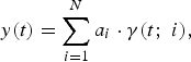 $$y\lpar t\rpar =\sum\limits_{i=1}^N {a_i \cdot \gamma \lpar t\semicolon \; i\rpar }\comma \; \eqno\lpar 5\rpar$$
where γ(t;i) are basis waveforms that are derived from nonlinear modes of the analog input signal x(t), a i are complex coefficients, and N is the number of basis waveforms in the PA model. In this paper, three basis sets are considered: memoryless polynomial, memory polynomial, and the Volterra series.
The basis set for the memoryless polynomial is
 $$\gamma _p \lpar t\rpar =\left\vert {x\lpar t\rpar } \right\vert ^{p - 1} \cdot\, x\lpar t\rpar \comma \; \eqno\lpar 6\rpar$$
where p is the polynomial order. The PA model is
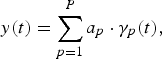 $$y\lpar t\rpar =\sum\limits_{p=1}^P {a_p \cdot \gamma _p \lpar t\rpar }\comma \; \eqno\lpar 7\rpar$$
where a p are complex coefficients and P is the highest polynomial order considered. The even-order terms (p = 2, 4, …) are often omitted from the basis set because the even-order distortion products are suppressed at the output of the PA by the transmit filter. However, ignoring the even terms is done more for convenience than necessity because it has been shown in [Reference Ding3] that including them in the baseband model can improve DPD performance.
The basis set for the memory polynomial is
 $$\gamma _p \lpar t\semicolon \; m\rpar =\gamma _p \lpar t - m\Delta \rpar =\left\vert {x\lpar t - m\Delta \rpar } \right\vert ^{p - 1} \cdot \,x\lpar t - m\Delta \rpar \comma \; \eqno\lpar 8\rpar$$
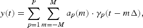
where m is an integer index and Δ is the delay offset between memory taps. The PA model becomes
 $$y\lpar t\rpar =\sum\limits_{p=1}^P {\sum\limits_{m=- M}^M {a_p \lpar m\rpar \cdot \gamma _p \lpar t - m\Delta \rpar \comma \; } } \eqno\lpar 9\rpar$$
where a p(m) are coefficients and M is the memory depth. Note that the memory depth M may vary with the polynomial order p.
The Volterra series is also a nonlinear representation with memory. The basis waveforms for polynomial order p = 3 and memory depth of M are
 $$\eqalignno{\gamma _3 \lpar t\semicolon \; m_1\comma \; m_2\comma \; m_3 \rpar & =x\lpar t - m_1 \Delta \rpar \cdot x\lpar t - m_2 \Delta \rpar\cr &\quad \cdot x^{\ast} \lpar t - m_3 \Delta \rpar \comma \; &\lpar 10\rpar}$$
where –M ≤ m 1, m 2, m 3 ≤ M and ()* indicates complex conjugate. For notational convenience, the basis waveform γ p(t; m 1,…,m p) will be written as γ(t;i) where the index i is a function of the polynomial order p and the memory taps (m 1,…,m p). The basis waveforms for odd orders p ≥ 3 are
 $$\gamma \lpar t\semicolon \; i\rpar =A\lpar m_1\comma \; \ldots\comma \; m_{0.5\lpar p+1\rpar} \rpar \cdot A\lpar m_{0.5\lpar P+3\rpar}\comma \; \ldots\comma \; m_p \rpar ^{\ast} \eqno\lpar 11\rpar$$
where
 $$A\lpar m_l\comma \; \ldots\comma \; m_j \rpar =x\lpar t - m_l \Delta \rpar \cdot x\lpar t - m_{l+1} \Delta \rpar \cdots x\lpar t - m_j \Delta \rpar .\eqno\lpar 12\rpar$$
The nonlinear behavior of the amplifier at analog baseband is modeled using
 $$y\lpar t\rpar =\sum\limits_{p=1}^P {\sum\limits_{m1=- M}^M { \cdots \sum\limits_{mp=- M}^M {a_i \cdot \gamma \lpar t\semicolon \; i\rpar } } } .\eqno\lpar 13\rpar$$
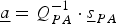
Consider the general form of the nonlinear model defined by (5). The estimate of the coefficients a i, based on the analog output y(t), is
 $$\underline a=Q_{PA} ^{ - 1} \cdot \underline s _{PA} \eqno\lpar 14\rpar$$
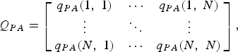
where a = [a 1…a N]T, sPA = [s PA(1)…s PA(N)]T, and
 $$Q_{PA}=\left[{\matrix{ {q_{PA} \lpar 1\comma \; 1\rpar } & \cdots & {q_{PA} \lpar 1\comma \; N\rpar } \cr \vdots & \ddots & \vdots \cr {q_{PA} \lpar N\comma \; 1\rpar } & \cdots & {q_{PA} \lpar N\comma \; N\rpar } \cr } } \right]\comma \; \eqno\lpar 15\rpar$$
 $$q_{PA} \lpar i\comma \; j\rpar =\vint {\gamma \lpar t\semicolon \; i\rpar \cdot \gamma ^{\ast} \lpar t\semicolon \; j\rpar \, \partial t\comma \; } \eqno\lpar 16\rpar$$
 $$s_{PA} \lpar i\rpar =\vint {y\lpar t\rpar \cdot \gamma ^{\ast} \lpar t\semicolon \; i\rpar\, \partial t} .\eqno\lpar 17\rpar$$
The cross-correlations of the basis waveform pairs q PA(i,j) determine the conditioning of the coefficient estimation. The condition number of Q PA is used later in Section IV for memory-based representations as a means of selecting the appropriate delay offset Δ.
III. BACK PROJECTING THE RF NONLINEARITY TO DIGITAL BASEBAND
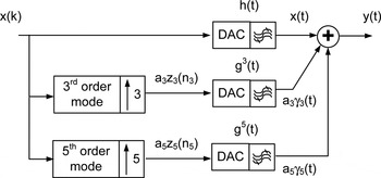
It is possible to back project the RF nonlinearity associated with the PA into the digital baseband, as shown in Fig. 2. This is done for each of the memoryless polynomial (Section III A), memory polynomial (Section III B), and Volterra series (Section III C) models. Information regarding the sampling rate needed to represent a nonlinear mode digitally is derived as a function of the polynomial order p. For the memory polynomial, the delay offset between memory taps Δ is specified as a function of p.
The analog baseband output signal y(t) is represented as a nonlinear function of the digital input x(k). The RF nonlinearity associated with the power amplifier is back-projected into the digital domain. Note that the sample rates for the digital sequences z 3(n 3) and z 5(n 5) are three and five times higher than the sample rate associated with x(k), as discussed later.

Although Fig. 2 shows the model of the PA nonlinearity back projected to the digital baseband, it is of greater interest to represent the inverse of the PA nonlinearity when performing DPD which projects the nonlinearity forward from digital into the RF domain. However, whether one projects nonlinearities forward or backward between the digital and RF domains, the required sampling rate and delay offset for nonlinear modes of x(k) are the same.
A) Memoryless polynomial
The basis waveforms for the memoryless polynomial, represented as a function of the digital input signal x(k), are written as (substitute (1) into (6))
 $$\gamma _p \lpar t\rpar =\left\vert {\sum\limits_k {x\lpar k\rpar\, h\lpar t - kT\rpar } } \right\vert ^{p - 1} \cdot \sum\limits_k {x\lpar k\rpar \, h\lpar t - kT\rpar } .\eqno\lpar 18\rpar$$
However, making sense of (18) in its current form is challenging. Consider the 3rd order mode, for example. Expanding (18) creates higher-order interpolation kernels of the form h(t − k 1T)*h(t − k 2T)*h(t − k 3T), which are difficult to interpret analytically. For simplicity, it will be assumed that the effective interpolation functions for the 3rd- and 5th-order modes are h 3(t) and h 5(t).
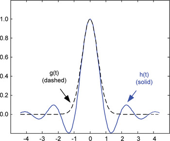
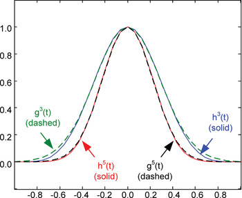
Assume the interpolation function for the linear mode, h(t), is a root raised cosine (RRC) with a roll-off factor of 0.22 (as is used for a single carrier WCDMA waveform). The function h p(t) becomes narrower in time as the polynomial order p increases. In addition, the sinc function shape of h(t), shown in Fig. 3, gradually takes on a Gaussian shape for h 3(t) and h 5(t), shown in Fig. 4. The Gaussian function has desirable properties for evaluating nonlinear modes, which are discussed later. As a result, the interpolation functions h p(t) for p ≥ 3 are assumed to have Gaussian shapes in order to make the mathematics associated with (18) tractable.
RRC function h(t) and the best-fit Gaussian approximation g(t).

Third- and fifth-order modes of the RRC function (h 3(t) and h 5(t)) and their Gaussian approximations (g 3(t) and g5(t)).

Let us first look at the validity of the Gaussian assumption. The comparison of the linear interpolation function h(t) to a Gaussian is shown in Fig. 3. The Gaussian fit to h(t) is a crude approximation at best. In contrast, the Gaussian approximations for the 3rd- and 5th-order modes are much better, as shown in Fig. 4. Thus, it is assumed that the information derived from using Gaussian interpolation functions is valid for the higher-order nonlinear modes (p ≥ 3).
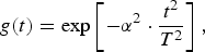
A Gaussian function is defined by
 $$g\lpar t\rpar =\exp \left[{ - \alpha ^2 \cdot \displaystyle{{t^2 } \over {T^2 }}} \right]\comma \; \eqno\lpar 19\rpar$$
where α is selected to best fit the Gaussian to the interpolation function h(t). Substituting g(t) for h(t) within (18), we have
 $$\gamma _p \lpar t\rpar =\left\vert {\sum\limits_k {x\lpar k\rpar \, g\lpar t - kT\rpar } } \right\vert ^{p - 1} \sum\limits_k {x\lpar k\rpar \, g\lpar t - kT\rpar } .\eqno\lpar 20\rpar$$
A simplification of (20) is possible because of the desirable properties of Gaussian functions: g(t) = g*(t) = |g(t)| and the product of Gaussians is also a Gaussian (narrower in time).
Equation (20) contains the product of p Gaussians, which can be written as
 $$g\lpar t - k_1 T\rpar \cdots g\lpar t - k_p T\rpar =g^p \left({t - n \cdot \displaystyle{T \over p}} \right)\cdot r_p \lpar \tau ^2 \rpar \comma \; \eqno\lpar 21\rpar$$
where
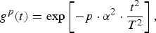 $$g^p \lpar t\rpar =\exp \left[{ - p \cdot \alpha ^2 \cdot \displaystyle{{t^2 } \over {T^2 }}} \right]\comma \; \eqno\lpar 22\rpar$$
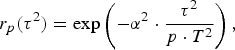 $$r_p \lpar \tau ^2 \rpar =\exp \left({ - \alpha ^2 \cdot \displaystyle{{\tau ^2 } \over {p \cdot T^2 }}} \right)\comma \; \eqno\lpar 23\rpar$$
 $$n=\sum\limits_{i=1}^p {k_i }\comma \; \eqno\lpar 24\rpar$$
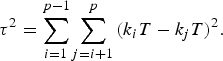 $$\tau ^2=\sum\limits_{i=1}^{p - 1} {\sum\limits_{j=i+1}^p {\lpar k_i } } T - k_j T\rpar ^2 .\eqno\lpar 25\rpar$$
Even though the sampling interval of the linear mode is T, the product of Gaussians, g(t − k 1T)…g(t − k pT), creates new Gaussians, g p(t − nT/p), some of which fall between the samples kT. Note that the index n in (21) is different for each polynomial order p.
For an odd order p, we can write (20) as
 $$\gamma _p \lpar t\rpar =\sum\limits_n^{} {z_p \lpar n\rpar \cdot g^p \left({t - n \cdot \displaystyle{T \over p}} \right)}\comma \; \eqno\lpar 26\rpar$$
where
 $$z_p \lpar n\rpar =\sum\limits_{k1=- \infty }^\infty { \cdots \sum\limits_{k\lpar p - 1\rpar =- \infty }^\infty {C\lpar k_1\comma \; \ldots\comma \; k_p \rpar } } \cdot r_p \left({\tau ^2 } \right)\comma \; \eqno\lpar 27\rpar$$
 $$C\lpar k_1\comma \; \ldots\comma \; k_p \rpar =x\lpar k_1 \rpar \cdot \prod\limits_{i=2}^{\lpar p+1\rpar /2} {x\lpar k_i \rpar \cdot x^{\ast} \lpar k_{i+\lpar p - 1\rpar /2} \rpar } .\eqno\lpar 28\rpar$$
Note that z p(n) is a sampled sequence and g p(t) is an interpolation function for the polynomial order p. The sampled sequence z p(n) contains p times more samples than the linear sequence x(k) from which it is derived. The interpolation function g p(t) is narrower in time than the linear function h(t). The term r p(τ2) defined in (23) reduces the influence of products of widely-spaced Gaussians providing a practical bound for the infinite summations in (27). It acts as a window that limits the summation to values of C(k 1,…,k p), where [(k 1 − k 2), (k 1 − k 3),…,(k p−1 − k p)] are close to [0, 0,…,0].
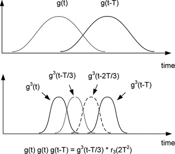
The first observation made from (26) is that the pth-order basis waveform γ p(t) is derived from a sampled sequence z p(n) whose sampling rate is p times higher than the linear mode (i.e., the sample period is T/p). To understand how this occurs, consider the 3rd order products of two Gaussians, g(t) and g(t − T). The resulting Gaussians (narrower in time) are centered at t = 0, t = T/3, t = 2T/3, and t = T, as shown in Fig. 5. Thus, despite the fact that z 3(n) is derived from x(k), the sequence z 3(n) has three times as many samples as the sequence x(k). Although the samples of z 3(n) are not independent of each other, a higher sampling rate (triple) is required to represent the 3rd-order nonlinear mode correctly because there is no linear dependency between samples of z 3(n) (assuming the samples of x(k) are independent). A similar requirement for higher sampling rates (by a factor of p) exists for any nonlinear mode p.
The sampling density is tripled for p = 3 over the linear mode. This is due to the cross-products g(t)g(t)g(t − T) and g(t)g(t − T)g(t − T) which create Gaussians located at t = T/3 and t = 2T/3, respectively.

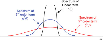
A second observation is that the interpolation function for the nonlinear mode p is g p(t). The spectra for the linear, 3rd-order, and 5th-order interpolation functions (h(t), g 3(t), and g 5(t)) are shown in Fig. 6. The width of the spectrum increases with the polynomial order p. Thus, it is important that any filters present in the analog or RF sections between x(t) and the PA output have sufficient bandwidth to pass the spectrum of the highest polynomial order of interest.
The spectrum of the linear interpolation function h(t) as well as the spectra of the third- and fifth-order functions, g 3(t) and g 5(t).

A third observation, made from (23) and (27), is that the term r p(τ2) becomes wider as p increases. This means that the influence of a symbol x(k) spreads out further in time for the higher orders of p. This may have an impact on the crest factor of the distorted signal. That is, several small perturbations of x(k) over a wide time period, performed in a coordinated manner, have the potential to enhance or attenuate a narrow peak within a nonlinear mode. However, it is not yet apparent to the author how this could be implemented as a crest factor reduction technique.
B) Memory polynomial
Now let us consider the memory polynomial. The memory polynomial in (8) can be written as
 $$y\lpar t\rpar =\sum\limits_{p=1}^P {a_p \cdot \sum\limits_{m=- M}^M {b_p \lpar m\rpar \cdot \gamma _p \lpar t - m\Delta \rpar \comma \; } } \eqno\lpar 29\rpar$$
where b p(m) = a p(m)/a p. Substituting (26) into (29), we get
 $$y\lpar t\rpar =\sum\limits_{p=1}^P {a_p \cdot \sum\limits_n {z_p \lpar n_p \rpar\, \cdot\, } } f_p \left({t - n \cdot \displaystyle{T \over p}} \right).\eqno\lpar 30\rpar$$
where f p(t) is the memory polynomial interpolation function for the nonlinear mode p and is defined as a weighted sum of offset Gaussians,
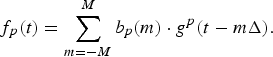 $$f_p \lpar t\rpar =\sum\limits_{m=- M}^M {b_p \lpar m\rpar \cdot g^p \lpar t - m\Delta \rpar } .\eqno\lpar 31\rpar$$
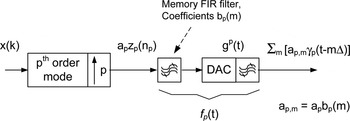
It is interesting to note from (30) that the memory polynomial has the same sampled sequence z p(n) as in the memoryless polynomial (see (27)). Equation (31) indicates that the memory polynomial modifies the interpolation functions used for the nonlinear modes, as shown in Fig. 7.
The pth order nonlinear mode of the memory polynomial.

The delay offset Δ can be selected arbitrarily. A small value of Δ increases the accuracy in which f p(t) is represented. However, some moderation is recommended because the incremental improvement in the accuracy diminishes as Δ is reduced. A small value of Δ also causes the estimation of the memory filter coefficients b p(m) to be ill-conditioned. In addition, it increases the number of basis waveforms needed to represent f p(t). Thus, there is a trade-off between accuracy, conditioning, and computational cost when selecting Δ.
The delay offset Δ and the polynomial order p affect the estimation of the memory filter coefficients b p(m). The estimate of b p(m) for a given order p is
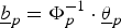 $$\underline b _p=\Phi _p ^{ - 1} \cdot \underline \theta _p \eqno\lpar 32\rpar$$
where bp = [b p(−M)…b p(M)]T, θ p = [θ p(−M)…θ p(M)]T, and
 $$\theta _p \lpar m_1 \rpar =\vint_{ - \infty }^\infty {f_p \lpar t\rpar \cdot g^p } \lpar t - m_1 \cdot \Delta \rpar \partial t\comma \; \eqno\lpar 33\rpar$$
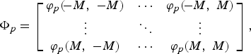 $$\Phi _p=\left[{\matrix{ {\varphi _p \lpar\! - M\comma \; - M\rpar } & \cdots & {\varphi _p \lpar\! - M\comma \; M\rpar } \cr \vdots & \ddots & \vdots \cr {\varphi _p \lpar M\comma \; - M\rpar } & \cdots & {\varphi _p \lpar M\comma \; M\rpar } \cr } } \right]\comma \; \eqno\lpar 34\rpar$$
 $$\varphi _p \lpar m_1\comma \; m_2 \rpar =\vint_{ - \infty }^\infty {g^p \lpar t - m_1 \cdot \Delta \rpar \cdot g^p \lpar t - m_2 \cdot \Delta \rpar \partial t} .\eqno\lpar 35\rpar$$
Elements of the matrix Φp, denoted by ϕ p(m 1, m 2), represent the overlap between Gaussian functions. The overlap is expressed as
 $$\varphi _p \lpar m_1\comma \; m_2 \rpar =S_p \cdot \exp \left[{ - \displaystyle{p \over 2} \cdot \alpha ^2 \cdot \lpar m_1 - m_2 \rpar ^2 \cdot \left\{{\displaystyle{\Delta \over T}} \right\}^2 } \right]\comma \; \eqno\lpar 36\rpar$$
where
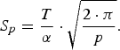 $$S_p=\displaystyle{T \over \alpha } \cdot \sqrt {\displaystyle{{2 \cdot \pi } \over p}} .\eqno\lpar 37\rpar$$
Note the (36) is a function of both Δ/T and p.
Equation (32) contains the inverse of the matrix Φp. As a result, the condition number of Φp becomes important. It is determined by ϕ p(m 1, m 2), which in turn is determined by the ratio Δ/T. Thus, the selection of Δ is still a trade-off between the accuracy in representing f p(t) and the condition number of Φp. An example showing this trade-off is presented in Section IV.
Almost all implementations of the memory polynomial used in DPD applications specify the same Δ for each p. This means that the accuracy and condition number trade-off is applied differently for each polynomial order p. It is the author's belief that the condition number of the matrix Φp should be the same for each p. To achieve this goal, Δ should decrease with the square root of the order p: that is,
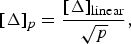 $$\lsqb \Delta \rsqb _p=\displaystyle{{\lsqb \Delta \rsqb _{{\rm linear}} } \over {\sqrt p }}\comma \; \eqno\lpar 38\rpar$$
where [Δ]linear and [Δ]p are the delay offsets for the linear mode and pth-order mode of the memory polynomial, respectively.
In summary, the first observation made is that the memory polynomial has the same digital sequences z p(n) as the memoryless polynomial but uses a different interpolation function where f p(t) replaces g p(t). As a result, the sampling interval for the pth order basis waveforms γ p(t − mΔ) is T/p, as in the memoryless polynomial case.
A second observation is that the delay offset should decrease as a function of p −0.5. Assuming the sample rate has already been increased by p to accommodate the pth order basis waveforms γ p(t − mΔ), it should not be problematic to implement different offsets for each p. However, it is shown in the next section that the pruned Volterra series provides an alternative method of increasing the sampling density associated with Δ as a function of p.
A third observation is that the choice between using a memoryless or memory polynomial is determined by Δ/T. Assume the memory of the PA can be model using two memory taps that are offset by Δ. The memoryless polynomial can be used successfully if the sample rate (and bandwidth) of the input signal is small enough that Δ/T is negligible. However, the memory of the PA must be modeled if the sample rate (and bandwidth) of the input signal increases. Thus, more detailed PA models are required for wider bandwidth input signals.
It is important to remember that the sampling interval T/p and the delay offset Δ are decoupled. The term T/p represents the effective sampling interval for an individual basis waveform. The delay offset Δ represents the sampling interval of the PA memory model provided by the basis set.
C) Volterra series
The Volterra series provides a detailed representation of PA nonlinearities. In general, it generates far more basis waveforms than needed for modeling the nonlinear modes of a band-limited signal. As a result, the Volterra series is often pruned to make the basis set size more manageable [Reference Zhu, Pedro and Cunba4–Reference Staudinger, Nanan and Wood6]. In this section, we look for guidance on how to best prune the set.
Consider the case for the polynomial order p. The basis waveforms are
 $$\eqalign{\gamma \lpar t\semicolon \; i\rpar & =x\lpar t - m_1 \Delta \rpar\, \cdot \prod\limits_{\phi=2}^{\lpar p+1\rpar /2} {x\lpar t - m_\phi \Delta \rpar } \cr & \quad\cdot x^{\ast} \lpar t - m_{\phi+\lpar p - 1\rpar /2} \Delta \rpar .} \eqno \lpar 39\rpar$$
The product of p Gaussians is
 $$\prod\limits_{i=1}^p {g\lpar t - k_i T - m_i \Delta \rpar }=g^p \left[{t - n \cdot \displaystyle{T \over p}+\mu \cdot \displaystyle{\Delta \over p}} \right]\cdot r_p \lpar \tau ^2 \rpar \comma \; \eqno\lpar 40\rpar$$
where
 $$\mu=\sum\limits_{i=1}^p {m_i }\comma \; \eqno\lpar 41\rpar$$
 $$n=\sum\limits_{i=1}^p {k_i }\comma \; \eqno\lpar 42\rpar$$
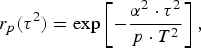 $$r_p \lpar \tau ^2 \rpar =\exp \left[{ - \displaystyle{{\alpha ^2 \cdot \tau ^2 } \over {p \cdot T^2 }}} \right]\comma \; \eqno\lpar 43\rpar$$
 $$\tau ^2=\sum\limits_{\phi=1}^{p - 1} {\sum\limits_{\delta=\phi+1}^p {\lpar k_\phi T} } - k_\delta T+m_\phi \Delta - m_\delta \Delta \rpar ^2 .\eqno\lpar 44\rpar$$
The basis waveforms can be rewritten as
 $$\gamma \lpar t\semicolon \; i\rpar =\sum\limits_n {z_p \lpar n_i\semicolon \; i\rpar \cdot g^p \left[{t - \displaystyle{{n_i \cdot T} \over p} - \displaystyle{{\mu _i \cdot \Delta } \over p}} \right]}\comma \; \eqno\lpar 45\rpar$$
where
 $$z_p \lpar n_i\semicolon \; i\rpar =\sum\limits_{k1}^{} { \cdots \sum\limits_{k\lpar p - 1\rpar }^{} {C\lpar k_1\comma \; \ldots\comma \; k_p \rpar } } \cdot r_p \lpar \tau _i ^2 \rpar \comma \; \eqno\lpar 46\rpar$$
 $$C\lpar k_1\comma \; \ldots\comma \; k_p \rpar =x\lpar k_1 \rpar \cdot \prod\limits_{i=2}^{\lpar p+1\rpar /2} {x\lpar k_i \rpar \cdot x^{\ast} \lpar k_{i+\lpar p - 1\rpar /2} \rpar } .\eqno\lpar 47\rpar$$
The sampling rate for a given basis waveform γ(t, i) increases by p, as can be seen by the T/p term in (40). In addition, the Gaussian interpolation function g p is offset relative to the memoryless polynomial case by μΔ/p, as seen in (45). What this means is that the individual basis waveforms γ(t, i) have the same sampling period (T/p); however, the digital sequences can be offset fractionally relative to each other. The basis set can be viewed as a polyphase sampling of the nonlinear PA memory, providing a higher sampling density compared with the basis set used in the memory polynomial.
Consider, as an example, the case where p = 3. The memory polynomial offsets are restricted to μ = 3m 1, whereas the Volterra series can select values of (m 1, m 2, m 3) = (m 1, m 1, m 1), (m 1 + 1, m 1, m 1), or (m 1, m 1 + 1, m 1 + 1), which correspond to μ = 3m 1, 3m 1 + 1, and 3m 1 + 2, respectively. The fractional offsets, μΔ/3, increase the effective sampling density of the Volterra series model relative to that of the memory polynomial.
The Volterra series is useful because additional basis waveforms are available. As mentioned earlier, it is desirable to have a similar condition number of Q PA for each order p. As a result, it is recommended that the pruned Volterra series retain the basis waveforms that are common to the memory polynomial, as well as a sufficient number of basis waveforms whose time offsets μiΔ/p fall between m φΔ to balance the sampling density for each order p, thereby fulfilling (38).
Pruning of the Volterra series can be done in many ways. The author's preference is to group conjugate terms together when selecting delay offsets. For example, the basis waveform set for an odd order p could have the form
 $$\gamma \lpar t\semicolon \; i\rpar =x\lpar t - m_1 \Delta \rpar \cdot \prod\limits_{i=2}^{\lpar p - 1\rpar /2} {\left\vert {x\lpar t - m_i \Delta \rpar } \right\vert ^2 } .\eqno\lpar 48\rpar$$
Equation (48) has fewer basis waveforms available compared with a Volterra series; however, it is still a very descriptive representation which requires further pruning.
The approach recommended is to select one's favorite basis set as a starting point, such as the memory polynomial, and fill in between using basis waveforms conforming to (48) to achieve a sampling density satisfying (38). One such basis set is listed in Table 1, where the neighboring basis waveforms are selected such that μ = Σm i differs by one. Note that m 1 and m 2 can be inter-changed for p = 3. Similarly, for p = 5, the tap indices m 1, m 2, and m 3 are interchangeable, as are m 4 and m 5. Note that the basis set described in Table 1 over-samples Δ for a given order p compared with (38). However, one can puncture the set to better approximate (38), if desired.
Basis waveform set for a pruned Volterra series conforming to (48).

D) Comparison
It is interesting to compare the structure of the memoryless polynomial, defined by (25–28), with that of the Volterra series, defined by (44–47). The similarity is due to the band limiting of the input signal x(k). The main differences are the terms (m φΔ − m δΔ) in (44) and the μ iΔ/p term in (45).
For the case of the memory polynomial, where m φ = m δ (see (44)), the basis waveforms γ(t;i) are time-shifted versions of the memoryless polynomial basis waveforms. Thus, as mentioned earlier, the memory polynomial can be viewed as a memoryless polynomial where each order p is followed by an adjustable FIR filter that alters the frequency response of interpolation function.
The basis waveforms of the pruned Volterra series are also time-shifted (by μ iΔ/p), where the density of the time shifts can be increased by as much as a factor of p compared with the memory polynomial. However, the Volterra series is not equivalent to an over-sampled memory polynomial because m φ ≠ m δ making τ 2 of (44) different from (25), which in turn changes the sequence z p(n) (compare (27) and (46)).
IV. EXAMPLES
In the following, examples of the memory polynomial (Section IV A) and the pruned Volterra series (Section IV B) are presented. The offset Δ is shown to affect both nonlinear representations as predicted in the previous section. A DPD example is provided in Section IV C which compares the linearization performance of the memory polynomial and pruned Volterra series for various offsets Δ.
Over-sampling a basis set by selecting a small offset Δ improves the accuracy of a nonlinear representation, assuming that the coefficients ai have been selected correctly (see (13)). However, because x(t) is band limited, there is a point where reducing Δ further will not produce a significant improvement in the accuracy of the nonlinear model of the PA or the performance of DPD.
Problems associated with over-sampling are more severe for the coefficient estimator. The coefficients are estimated based on the input signal x(k) and the observed output signal y(k). The condition number of Q PA drops when the basis set over-samples the memory space. In such cases, the coefficient estimation will be ill-conditioned and susceptible to noise in the observed output signal y(k).
Although the condition number is useful, it is often preferable to look at the distribution of the eigenvalues of Q PA to determine the best offset Δ. This is the case because singular value decomposition (SVD) can be used to remove the influence of eigenvectors associated with the smallest eigenvalues. As a result, the number of eigenvalues below the SVD threshold is a good indication of the degree of over-sampling of Δ within the basis set.
To better understand SVD, consider the inverse of Q PA (see (14)). It can be written as
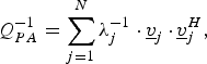 $$Q_{PA} ^{ - 1}=\sum\limits_{j=1}^N {\lambda _j ^{ - 1} \cdot \underline v _j \,\cdot\, } \underline v _j ^H\comma \; \eqno\lpar 49\rpar$$
where λ j and vj are the eigenvalues and eigenvectors of Q PA, respectively. It is assumed that the eigenvalues λ j are ordered by descending values so that λ N denotes the smallest. The projection of y(t) onto the basis waveforms γ(t;i), defined earlier by (17), can also be written as a weighted sum of eigenvectors: that is,
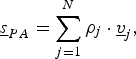 $$\underline s _{PA}=\sum\limits_{j=1}^N {\rho _j \cdot \underline v _j }\comma \; \eqno\lpar 50\rpar$$
where ρ j are complex coefficients. The nonlinear mode associated with the eigenvector vN is difficult to observe within the output signal y(t) using the estimator in (14) when the basis set is over-sampled. As a result, the coefficient ρ N in (50) will be very small. This is compensated during the coefficient estimation (14) by the large gain provided by λ N−1. However, any noise introduced onto ρ N will be enhanced. A SVD threshold λSVD is applied to prevent such condition problems from occurring. SVD replaces λ j−1 with zero in (49) when λ j < λSVD. For DPD systems, the SVD threshold is often selected by trial-and-error to optimize the linearization performance.
We require an input signal for the following examples. Let us create a band limited input signal x(t) from which the matrix Q PA can be computed. Random complex samples with a Gaussian distribution are generated to produce the digital sequence x(k). It is up-sampled by a factor of eight by inserting seven zeroes between samples. The over-sampled digital sequence is low-pass filtered using a root raised cosine. The resulting band limited sequence is used to compute the basis waveforms γ(t;i). The offset Δ is selected to be a multiple of T/8.
The matrix Q PA, in practice, contains the cross-correlations of basis waveforms from all polynomial orders p. However, in the following, the 3rd- and 5th-order modes are viewed in isolation to determine the appropriate offset Δ and to verify the theory presented in Section III.
A) Memory polynomial
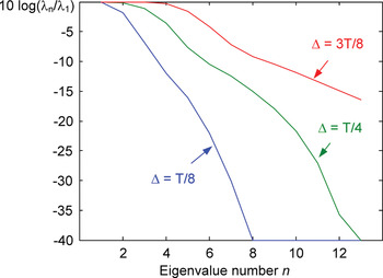
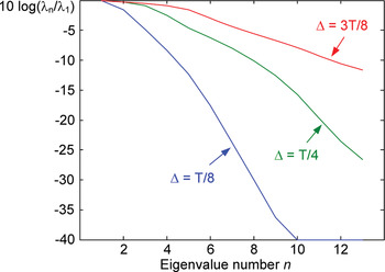
Let us consider the case of the memory polynomial where the memory depth is M = 6 for the 3rd order basis set, |x(t − mΔ)|2x(t − mΔ). Since negative tap indices are included, −M ≤ m ≤ M, Q PA has 13 eigenvalues. The eigenvalue distribution is shown in Fig. 8 for the cases of Δ = T/8, T/4, and 3T/8. The SVD threshold is selected to be 0.0001 of the largest eigenvalue. The best choice for the offset Δ is the smallest value that retains most of the eigenvalues (that is, most λ i > λSVD). Thus, Δ = T/4 is a good choice because the smallest eigenvalue λ13 approaches the SVD threshold without falling below it (see Fig. 8).
The eigenvalue (λ n) distribution of Q PA for the third-order mode of a memory polynomial using different offsets Δ. The eigenvalues are ordered in descending value and normalized by the dominant eigenvalue λ1. A RRC filter is applied to input signal x(k).

The matrix Q PA for the 3rd-order mode, using a RRC filter and an offset of Δ = T/4, is
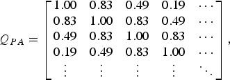 $$Q_{PA}=\left[{\matrix{ {1.00} & {0.83} & {0.49} & {0.19} & \cdots \cr {0.83} & {1.00} & {0.83} & {0.49} & \cdots \cr {0.49} & {0.83} & {1.00} & {0.83} & \cdots \cr {0.19} & {0.49} & {0.83} & {1.00} & \cdots \cr \vdots & \vdots & \vdots & \vdots & \ddots \cr } } \right]\comma \; \eqno\lpar 51\rpar$$
The matrix Q PA has a band structure which decays with the off-diagonal distance. Smaller values of the offset Δ have a slower decay off-diagonal as predicted by (36).
Let us make a comparison to the theory presented in Section III. The cross-correlations q PA(i, j) found in (51) are similar to the Gaussian filter results based on (36): q PA(1,2) = 0.85, q PA(1,3) = 0.56, and q PA(1,4) = 0.33 (note the q PA(1,2) corresponds to the cross-correlation of γ 3(t;m 1, m 2, m 3) and γ 3(t;m 1 + 1,m 2 + 1,m 3 + 1)). The Gaussian filter is a good estimate of the RRC results for the elements close to the diagonal. However, the difference becomes larger with the off-diagonal distance.
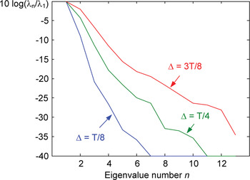
The memory depth for 5th order basis set, |x(t − mΔ)|4x(t − mΔ), is also M = 6. The eigenvalue distribution of Q PA for the 5th-order mode is shown in Fig. 9 for the cases of Δ = T/8, T/4, and 3T/8. The SVD threshold is selected to be 0.0001 of the largest eigenvalue, as in the 3rd order case. An offset of Δ = T/4 is still a good choice. However, the 13th eigenvalue for the 5th-order mode is larger than that of the third order mode, which indicates that the sampling density is sparser for the 5th order mode, as predicted by (36).
The eigenvalue (λ n) distribution of Q PA for the fifth-order mode of a memory polynomial using different offsets Δ. The eigenvalues are ordered in descending value and normalized by the dominant eigenvalue λ1. A RRC filter is applied to input signal x(k).

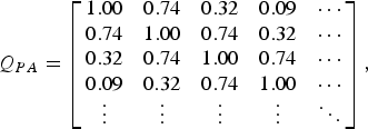
The matrix Q PA for the 5th-order mode, using a RRC filter and an offset of Δ = T/4, is
 $$Q_{PA}=\left[{\matrix{ {1.00} & {0.74} & {0.32} & {0.09} & \cdots \cr {0.74} & {1.00} & {0.74} & {0.32} & \cdots \cr {0.32} & {0.74} & {1.00} & {0.74} & \cdots \cr {0.09} & {0.32} & {0.74} & {1.00} & \cdots \cr \vdots & \vdots & \vdots & \vdots & \ddots \cr } } \right]\comma \; \eqno\lpar 52\rpar$$
The elements q PA(i, j) decay off-diagonal, as in the 3rd-order case. However, the decay is more rapid for the 5th-order mode. This characteristic of the memory polynomial was predicted earlier by (36).
B) Pruned Volterra series
Consider an example based on the Volterra series, pruned using (48). Let us start by including basis waveforms common to a memory polynomial. The set for p = 3 and M = 2 includes (m 1, m 2, m 3) = (−2, −2, −2), (−1, −1, −1), (0,0,0), (1,1,1), and (2,2,2). The set for p = 5 and M = 1 includes (m 1,…,m 5) = (−1, −1, −1, −1, −1), (0,0,0,0,0), and (1,1,1,1,1). The pruned Volterra series is completed by adding basis waveforms listed in Table 1.
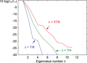
Filling in the memory polynomial using a pruned Volterra series creates a 3rd order set with 13 basis waveforms and 13 eigenvalues in Q PA. The eigenvalue distribution of Q PA is shown in Fig. 10 for the cases of Δ = T/8, T/4, and 3T/8. An offset of Δ = 3T/8 is a good choice for a SVD threshold of 0.0001 (see Fig. 10).
The eigenvalue (λ n) distribution of Q PA for the third-order mode of a pruned Volterra series using different offsets Δ. The eigenvalues are ordered in descending value and normalized by the dominant eigenvalue λ1. A RRC filter is applied to input signal x(k).

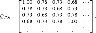
The matrix Q PA for the 3rd-order mode, using a RRC filter and an offset of Δ = 3T/8, is
 $$Q_{PA}=\left[{\matrix{ {1.00} & {0.78} & {0.73} & {0.68} & \cdots \cr {0.78} & {0.73} & {0.68} & {0.73} & \cdots \cr {0.73} & {0.68} & {0.73} & {0.78} & \cdots \cr {0.68} & {0.73} & {0.78} & {1.00} & \cdots \cr \vdots & \vdots & \vdots & \vdots & \ddots \cr } } \right].\eqno\lpar 53\rpar$$
The diagonal elements vary where the highest values correspond to the elements associated with the original memory polynomial. In addition, there is less decay off-diagonal than the memory polynomial case. This indicates denser sampling than would be suggested by looking at nearest off-diagonal elements, q PA(i, i + 1), only.
For the case of the 5th-order mode, the pruned Volterra series creates a basis set with 11 waveforms, which means that Q PA has 11 eigenvalues. The eigenvalue distribution is shown in Fig. 11 for the cases of Δ = T/8, T/4, and 3T/8. The SVD threshold is selected to be 0.0001. An offset of Δ = 3T/8 is still a good choice. The eleventh eigenvalue is closer to the SVD threshold than in the 3rd order case, which indicates that the sampling density is higher for the 5th order mode, as predicted by μΔ/p in (45).
The eigenvalue (λ n) distribution of Q PA for the fifth-order mode of a pruned Volterra series using different offsets Δ. The eigenvalues are ordered in descending value and normalized by the dominant eigenvalue λ1. A RRC filter is applied to input signal x(k).

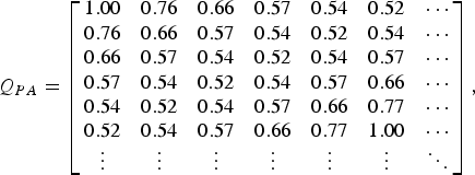
The matrix Q PA for the 5th order mode, using a RRC filter and an offset of Δ = 3T/8, is
 $$Q_{PA}=\left[{\matrix{ {1.00} & {0.76} & {0.66} & {0.57} & {0.54} & {0.52} & \cdots \cr {0.76} & {0.66} & {0.57} & {0.54} & {0.52} & {0.54} & \cdots \cr {0.66} & {0.57} & {0.54} & {0.52} & {0.54} & {0.57} & \cdots \cr {0.57} & {0.54} & {0.52} & {0.54} & {0.57} & {0.66} & \cdots \cr {0.54} & {0.52} & {0.54} & {0.57} & {0.66} & {0.77} & \cdots \cr {0.52} & {0.54} & {0.57} & {0.66} & {0.77} & {1.00} & \cdots \cr \vdots & \vdots & \vdots & \vdots & \vdots & \vdots & \ddots \cr } } \right]\comma \; \eqno\lpar 54\rpar$$
The diagonal elements vary where the highest values correspond to the elements associated with the original memory polynomial. There is little decay off-diagonal indicating a higher sampling density, as in the 3rd order case.
D) Digital predistortion
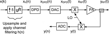
Let us consider a DPD example. The digital transmitter with predistortion is shown in Fig. 12. The input x(k) is a four-carrier WCDMA signal with a peak-to-average power ratio (PAPR) of 9.5 dB. It spans a bandwidth of approximately 20 MHz making T = 0.05 µs. The WCDMA carriers are up-sampled to 100 MHz, channel filtered digitally, and summed to create the signal x h(n). The DPD is applied using a pruned Volterra series:
 $$x_{DPD} \lpar n\rpar =x_h \lpar n\rpar +\sum\limits_{p=1}^P {\sum\limits_{m1=- M}^M { \cdots \sum\limits_{mU=- M}^M {c_i \cdot \gamma \lpar n\semicolon \; i\rpar \comma \; } } } \eqno\lpar 55\rpar$$
where
 $$\gamma \lpar n\semicolon \; i\rpar =x_h \lpar n - m_1 \rpar \cdot \prod\limits_{\phi=2}^U {\left\vert {x_h \lpar n - m_\phi \rpar } \right\vert ^2 }\comma \; \eqno\lpar 56\rpar$$
U = (p + 1)/2, the index i is a function of p and (m 1,…,m U), c i are DPD coefficients, and n is the time index representing the up-sampled signal (100 MHz).
Transmitter with DPD.

The DPD signal x DPD(n) is converted to an analog signal x DPD(t) using
 $$x_{ {DPD} } \lpar t\rpar =\sum\limits_n {x_{DPD} \lpar n\rpar \, h_{DAC} \lpar t - n \cdot T_n \rpar \comma \; } \eqno\lpar 57\rpar$$
where h DAC(t) is an interpolation function suitable for the 100 MHz sampling rate, and T n = 0.01 µs. The analog signal x DPD(t) is up-converted to RF and becomes the input to the PA, x RF(t). The PA output y RF(t) is down-converted and digitized to create y(n), which is used to measure the residual nonlinear behavior of the predistorted PA.
The estimate of the DPD coefficient errors Δc i minimizes
 $$J=\sum\limits_n {\left\vert {L\lcub \varepsilon _{DPD} \lpar n\rpar \rcub - \sum\limits_{i=1}^N {\Delta c_i \cdot L\lcub \gamma \left({n\semicolon \; i} \right)\rcub } } \right\vert ^2 }\comma \; \eqno\lpar 58\rpar$$
where
 $$\varepsilon _{DPD} \lpar n\rpar =G_o ^{ - 1} \cdot y\lpar n\rpar - x\lpar n\rpar \comma \; \eqno\lpar 59\rpar$$
L{} indicates the use of an estimation filter which attenuates (notches) the in-band frequencies (see [Reference Braithwaite and Carichner7–Reference Braithwaite and Carichner11] for details), and G o is the linear gain of the transmitter. The DPD coefficients are updated recursively using
 $$\underline c \lpar l+1\rpar =\underline c \lpar l\rpar - \eta \cdot \underline {\Delta c}\comma \; \eqno\lpar 60\rpar$$
where c = [c 1…c N]T, Δc = [Δc 1…Δc N]T, η < 1, and l is the iteration number.
The accuracy of the DPD for a WCDMA signal is measured by the residual out-of-band distortion within the digitized output signal y(n). In particular, the WCDMA standard [12] specifies maximum values for the adjacent channel leakage ratio (ACLR) of the output signal y(n), which are ACLR1 < −45 dBc and ACLR2 < −50 dBc.
Four basis sets, each containing 28 basis waveforms, are tested: a memory polynomial and three pruned Volterra series using different delay offsets Δ. Each set comprises a 7th-order memoryless polynomial including the even terms (p = [2–7]). The memory polynomial has memory depths of M = 6 for p = 3 and M = 5 for p = 5. The delay offset is Δ = 0.2T. The pruned Volterra series uses the set described in Table 1 with memory depths of M = 2 for p = 3 and M = 1 for p = 5. Three delay offsets are considered: Δ = 0.2T, 0.4T, and 0.6T.
The sampling rate of 100 MHz is not high enough to compute the p = 7 waveform used in the memoryless polynomial without aliasing. That is, a sampling rate of 140 MHz (7*20 MHz) is needed. To prevent aliasing, the sampling rate is doubled prior to computing the |x|6x waveform, then filtered and decimated by 2 to restore the original sampling rate. This technique is described in [Reference Shalom13] and [Reference Braithwaite2]. It is also used for the even-order terms of the memoryless polynomial because the |x|x, |x|3x, and |x|5x modes create wide bandwidths due to the square root operation used in computing the odd-order absolute value.
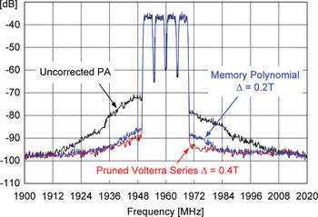
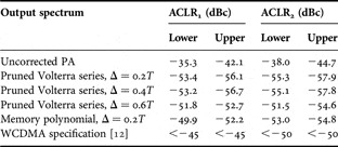
The output spectra for the uncorrected PA, the predistorted PA using the memory polynomial (Δ = 0.2T), and the pruned Volterra series (Δ = 0.4T) are shown in Fig. 13. The ACLR measurements appear in Table 2. The output spectrum for the uncorrected PA fails the ACLR specifications verifying the need for linearization. All four of the DPD basis sets predistort the PA sufficiently well to pass both ACLR1 (<−45 dBc) and ACLR2 (<−50 dBc). However, it is still of interest to compare the ACLR results for three pruned Volterra series (Δ = 0.2T, 0.4T, and 0.6T) with each other and with the memory polynomial (Δ = 0.2T).
Spectra for the uncorrected PA and for the predistorted PA using the memory polynomial (Δ = 0.2T) and the pruned Volterra series (Δ = 0.4T).

ACLR measurements for various output spectra.

There is little difference between the ACLR results for the pruned Volterra series when Δ = 0.2T or Δ = 0.4T (see Table 2). In contrast, increasing the delay offset to Δ = 0.6T causes a discernible degradation in the ACLR. This suggests that Δ = 0.2T is over-sampling the pruned Volterra basis set. This should not be surprising given that Figs 10 and 11 indicate that Δ = 3T/8 is a good choice for the pruned Volterra series basis set defined by Table 1.
Let us compare the pruned Volterra series for Δ = 0.4T with the memory polynomial (Δ = 0.2T). Despite using a larger offset Δ, the pruned Volterra series produces better ACLR results. The ACLR measurements for the memory polynomial (Δ = 0.2T) are comparable to those of the pruned Volterra series when Δ = 0.6T.
As part of the coefficient estimation, a matrix Q DPD is computed, which is similar in structure to Q PA defined by (15), whose elements are
 $$q_{DPD} \lpar i\comma \; j\rpar =\sum\limits_n {L\lcub \gamma \lpar n\semicolon \; i\rpar \rcub \cdot L\lcub \gamma ^{\ast} \lpar n\semicolon \; j\rpar \rcub } .\eqno\lpar 61\rpar$$
The condition numbers of Q DPD for the pruned Volterra series are 47N κ, 1.4N κ, and N κ for Δ = 0.2T, 0.4T, and 0.6T where N κ = 16 800. As expected, the condition number decreases as Δ becomes larger. The condition number for the memory polynomial is 253N κ, which is considerably larger than any of the pruned Volterra series.
The estimator uses SVD (see [Reference Braithwaite8] for details) to reduce the condition number of the memory polynomial to 0.87N κ. Experiments show that this does not degrade the ACLR. It is apparent that reducing the offset Δ below 0.2T will not improve DPD performance of the memory polynomial. This should not be surprising given that Fig. 8 and Fig. 9 indicate that Δ = T/4 is a good choice for the memory polynomial.
It is the author's opinion that the pruned Volterra series with Δ = 0.4T is the best trade-off of ACLR performance and condition number for this example. The basis set defined by Table 1 shows an improvement in terms of ACLR over the memory polynomial. This example illustrates how the sampling density of the basis set can be increased over the memory polynomial by adding Volterra series waveforms.
V. COMMENTS
Recommendations and future work are discussed in Section V A and Section V B, respectively.
A) Recommendations
Although the pruned Volterra series shows the best DPD performance in Fig. 13, it is recommended that simpler basis sets be used when the PA nonlinearity allows it. In general, one should start with a memory polynomial with a reasonable memory depth M (or other simple memory-based representation). The appropriate offset Δ is determined using the eigenvalues of Q PA, as shown earlier in Section IV. If the linearization performance is sufficient, the memory depth should be reduced until a target value of ACLR is reached (usually the WCDMA specification plus a manufacturing margin). If M = 0 meets the ACLR target, then use a memoryless polynomial. However, if the memory polynomial does not produce sufficient DPD performance, introduce new Volterra series waveforms into the basis set and adjust Δ accordingly. This will produce good linearization results while minimizing the number of basis waveforms used.
B) Future work
This work has investigated the sampling requirement for a band-limited input signal where the pass band is approximately flat. An extension of this work would be to investigate WCDMA carriers that are separated by idle channels [Reference Braithwaite14]. Each contiguous carrier cluster could be modeled using the Gaussian approximation and the intermodulation between carrier clusters could be modeled separately. The author anticipates the use of Gabor functions (modulated Gaussians) [Reference Gabor15] in such a future analysis.
VI. CONCLUSION
Nonlinear modes generated when a band-limited signal undergoes nonlinear amplification have been modeled using a Gaussian approximation. The model is shown to be accurate enough to determine mathematically the sampling rates needed to represent the nonlinear modes as digital baseband waveforms. It is shown that the sampling rate for nonlinear modes of odd order p must increase by a factor of p over the Nyquist rate of the linear mode to avoid aliasing. The mathematical analysis indicates that the coefficient estimation benefits when the delay offset Δ for the memory polynomial decreases in size as a function of the polynomial order p. A pruned Volterra series has been introduced where the distance between neighboring basis waveforms decreases with p, as desired. It is used for DPD, demonstrating improved performance over the memory polynomial.
 R. Neil Braithwaite received the B.Sc. degree in electrical engineering from the University of Calgary, Canada, in 1985, and the M.Sc. and Ph.D. degrees from the University of British Columbia, Canada, in 1989 and 1992, respectively. From 1992 to 1995, he conducted postdoctoral work at the University of California, Riverside. He has worked for Computing Devices Company (acquired by General Dynamics) in Ottawa, Canada, from 1985 to 1987, and Nortel in Calgary, Canada, from 1995 to 1997. From 1997 to 2002, he worked for Agilent Laboratories in Palo Alto, CA. He is currently working for Powerwave Technologies in Santa Ana, CA in the Research and Development group. His research interests include signal processing, linearization of RF power amplifiers, and echo cancelation in RF repeaters.