1. Introduction
Sustainable development is a concept of concern about the well-being of both present and future generations. It involves trade-offs between present and future use of environmental and natural resources. To address this intergenerational equity concern, various concepts of sustainability have been proposed since the publication of the ‘Brundtland Commission Report’ (WCED, 1987). These include economic approaches that are grounded on earlier works of Solow (Reference Solow1974), Hartwick (Reference Hartwick1977) and Daly (Reference Daly1972, Reference Daly1974), and encompass the integration of ecological concepts of resilience (Common and Perrings, Reference Common and Perrings1992), critical natural capital (Pearce et al., Reference Pearce, Atkinson and Dubourg1994) and basic needs (Chichilnisky, Reference Chichilnisky1977; Hediger, Reference Hediger1999) as well as the development of new approaches, such as Chichilnisky's (Reference Chichilnisky1996, Reference Chichilnisky1997) criterion to balance the short run with the long run future.Footnote 1
The dominant concern in most economic approaches to sustainable development is about the maintenance of current or optimal level of consumption or utility into the far distant future. Hence, much attention is given to the exhaustibility of natural resources and the challenge of maintaining some suitably defined stocks of capital. However, most models of sustainability do not explicitly consider the accumulation of pollutants in the environment, or, at least, not with the same rigour as in the environmental economics literature on optimal pollution control. The latter evolved since the publications of Keeler et al. (Reference Keeler, Spence and Zeckhauser1972) and Plourde (Reference Plourde1972). It covers various economic aspects of pollutant accumulation and control, such as the implication of different forms of the assimilation function, economic growth and the investment in clean technologies, and the problem of global warming. However, the relationship between trajectories of optimal pollution control and sustainable development has received little attention in published work, and has not been investigated in a comprehensive way.
Barbier and Markandya (Reference Barbier and Markandya1990) only identify the minimum initial level of environmental quality required to ‘ensure a sustainable growth path’, which is solely characterized by an increase of the total stock of environmental assets. However, they neither investigate the effects of the optimal trajectory upon the development of aggregate income and social welfare, nor are they explicit with regard to the accumulation and assimilation of pollution. In contrast, Chevé (Reference Chevé2000) elucidates the importance of a decline in the natural pollution decay function upon optimal pollution control and economic growth. But, her argumentation is restricted to the case of strong sustainability with a non-decreasing stock of natural capital that is simply represented by the stock of pollution. Hence, Chevé's conclusion that ‘a better environmental quality can be associated with higher economic growth’ is valid only for the case of an initial stock of pollution above the long-term optimum. This can be referred to as a problem of environmental restoration, rather than a general problem of optimal pollution control.
Hartwick (Reference Hartwick1997), in an extension of Becker's (Reference Becker1982) model, also reflects on sustainable development in situations with high initial stocks of pollution. Applying a weak sustainability framework of constant utility over time, he suggests that ‘reducing high pollution stocks can be interpreted as paying off the current debt in environmental capital’, which requires high-cleanup activities and lowers investment in physical and human capital. But, Hartwick does not investigate the impact on the trajectory of economic development, such as Chevé (Reference Chevé2000) that is also restricted to the case with high initial pollution stocks.
On the contrary, Stollery (Reference Stollery1998) investigates the existence of constant utility paths in the case of irreversible greenhouse gas accumulation from fossil fuel carbon emissions. Using a resource model where the fossil fuel stock is completely converted into the stock of atmospheric CO2 (assuming a zero rate of decay) and where the associated externality (global temperature increase) is declining with the remaining resource stock in the ground, Stollery shows that ‘a carbon tax is required to steer the economy along the sustainable path’ and that ‘the constant utility level is maximized by following the standard Hartwick rule’. The latter requires the global economy to invest in reproducible capital, the sum of the carbon tax revenues and after-tax resource rents, that is, the gross energy resource rent. In essence, this is exactly the same result as Hartwick (Reference Hartwick1977). In other words, it does not differ from the original Hartwick rule without consideration of pollution.Footnote 2 Yet, Hediger (Reference Hediger2006) shows that in the presence of stock pollution the standard Hartwick rule must be extended and include an additional term that does not vanish even if the stock of pollution would be kept constant over time. Hence, to comprehensively address the challenge of sustainable development and to be consistent our models must explicitly address the accumulation and decay of pollutants.Footnote 3
Altogether, this indicates the need of extending our research to more comprehensively address the problem of optimal pollution control and to pay attention to both problems of environmental restoration and continued pollution accumulation along the optimal time paths, and to evaluate the results from a sustainable development perspective.
Building on this background, the aim of the present paper is to provide an economic analysis of optimal pollution control and sustainable development, and to widen the above literature. To this end, we start with the rather general model of Forster (Reference Forster1975) and gradually extend this analytical framework to gain additional insights about the relationship between optimal pollution control and the sustainability of development. The basic model is introduced in section 2, while section 3 provides a first discussion of the optimal pollution control trajectories from both an efficiency and sustainability point of view. It shows that the existence of constant productive capacity is not in general sufficient for sustainable development. Rather, additional investments might be required to maintain a non-declining flow of consumption. Therefore, the model is extended in section 4 to jointly address optimal pollution control and capital accumulation. The extended model is also used in section 5 to investigate the option of a Hartwick-type investment rule as a means to facilitate a constant flow of welfare along an intertemporally optimal trajectory of pollution accumulation. This is also considered in brief from a perspective of sustainable preferences, as defined by Chichilnisky (Reference Chichilnisky1996, Reference Chichilnisky1997), and for the case of environmental restoration. Finally, section 6 concludes.
2. The basic model
The accumulation of pollutants is a major cause of environmental degradation and adverse impacts upon human health and welfare. Examples include soil and water contamination with toxic substances or sulphur and nitrogen compounds, the eutrophication of surface waters, as well as increased concentrations of greenhouse gases and ozone depleting substances in the atmosphere. For these substances, damages to ecosystems and human interests depend on the stock of pollution, which consequently has an adverse impact on social welfare. This is usually represented in the form of a concave utility function U of instantaneous consumption C and the current stock of pollution S, which has the following properties:

Following Forster (Reference Forster1975, Reference Forster, Pitchford and Turnovsky1977), the last two conditions are used for reasons of tractability and to rule out the unrealistic boundary solutions of zero consumption and zero pollution. Moreover, in line with Forster's model, we assume for the moment that the economy has a fixed productive capacity and that it produces a constant level of output  . This is allocated to consumption C and anti-pollution activities Z:Footnote 4

Assuming a constant and free flow of renewable resources, the dynamic problem in our analysis comes from the intertemporal accumulation of pollution

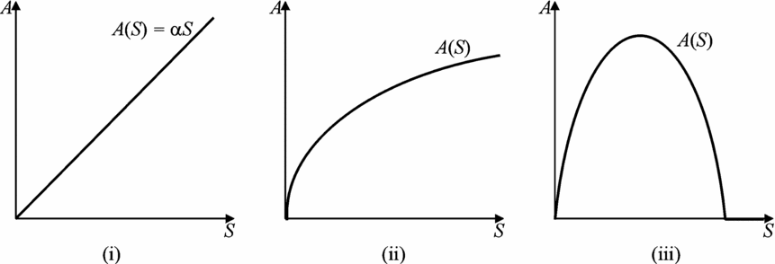
This is the excess flow of net emissions E(C) − G(Z), with E′ > 0, E′ > 0, G′ > 0 and G″ < 0, above the natural capacity of pollutant assimilation, the so-called assimilative capacity A(S). According to Pearce (Reference Pearce1976), the latter refers to the environment's capability of receiving waste, degrading it, converting it to nutrients for the occupants of the ecosystem or rendering it harmless to species even if the converted product is not required as an input to the ecosystem. Depending on the type of pollutant this essential natural function can take different forms, as illustrated in figure 1:Footnote 5
Different forms of the assimilation function
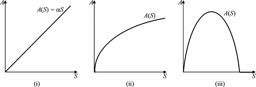
• Case (i) is the most often used functional form in the optimal pollution control literature. It is characterized by a constant proportionate rate of decay α, which would typically be the case for the decay of radioactive substances.
• Case (ii) is rarely used in the environmental economics literature. It describes the process of saturation that is typical for chemical processes of self-purification (cf. Fiedler, Reference Fiedler1994). It could also be an important representation of the global CO2 assimilative capacity, since the uptake of CO2 declines with the atmospheric concentration (Watson et al., Reference Watson, Noble, Bolin, Ravindranath, Verardo and Dokken2000) and the fraction of a unit emission of CO2 remaining in the atmosphere is higher the higher the accumulated emissions are (Azar, Reference Azar1995).
• Case (iii) is typical for biological processes of self-purification (cf. Fiedler, Reference Fiedler1994, Reference Fiedler1997) that are limited by some degrader populations (e.g., microorganisms) and general environmental conditions, such as the oxygen and other nutrients available to support the degraders. This functional form has first been used in the environmental economics literature by Forster (Reference Forster1975), and since then has gained increasing attention from other economists who are concerned about the influence of ecological processes upon the economy and their representation in economic analysis.
In this study, we concentrate on the third case which is the most interesting from an analytical point of view, and the most relevant from an ecological perspective. It combines the favourable case where the ecosystem's assimilative capacity increases with the stock of pollution for low levels and the adverse consequences of saturation. The latter results first in a decline of the marginal rate of assimilation, followed by continuous deterioration of the assimilative capacity for further pollution accumulation beyond a certain turning point, say Sm. This natural process ends with the complete destruction of the assimilative capacity at the pollution level S, beyond which this ecosystem function is reduced to zero.Footnote 6
Formally, the assimilation function can be represented as follows:

As indicated, if the net flow of emissions from the economy exceeds this capacity, the stock of pollution accumulates in the environment and has a negative impact upon the society's well-being. Hence, we face an intertemporal allocation problem. This is usually formalized in terms of maximizing the present value of instantaneous utility by choosing the optimal level of consumption
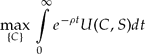
subject to  where ρ > 0 denotes the constant social discount rate and f(C) the economy's net emissions:

with f′ = E′ + G′ > 0, f″ = E″ − G′ > 0.
Using Pontryagin's maximum principle, this intertemporal optimization problem can be represented by the current-value Hamiltonian

which is to be maximized at each point in time. The following differential equations define the optimal time path of the state and costate variables, S and μ, of this allocation problem:


Along this trajectory the allocation of the existing output to consumption and pollution abatement must continuously be adjusted, so as to satisfy the capacity constraint (2) and the subsequent first-order condition at each point in time:

Using this optimality condition, it can be shown that the shadow price of pollution is strictly negative, which reflects that pollution generates disutility:

Moreover, using equations (1) and (2), respectively, it follows that

and thus

Consumption must develop with the same sign as the value of the costate variable μ, while the share of output allocated to pollution abatement must go in the opposite direction.
This is crucial for economic growth and sustainable development, but, so far, has not gained adequate attention in the literature and policy debate. To fill up this gap, we proceed in a straightforward manner by first investigating the relationship between optimal pollution control and sustainable development prospects within the framework of Forster's (1975) model with constant productive capacity, and then extend the analysis by relaxing the latter restriction.
3. Optimal pollution control with constant productive capacity
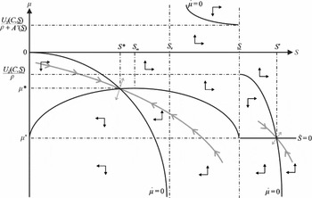
The solution of the above optimal control program is characterized by a steady state where  and a stable transition path from the initial state S 0 towards this long-term optimum. Yet, as Forster (Reference Forster1975) and Tahvonen and Withagen (1996) already pointed out, multiple equilibria can exist for the optimal pollution control problem with a biological assimilation function. One of these long-term optima implies an intact assimilative capacity A(S*) > 0. This is illustrated in figure 2 by the intersection of the
 and
 demarcation curves in the point (S*, μ*). Here S* denotes the optimal stock of pollution in the steady state and μ* the corresponding shadow price of pollution. The second long-term optimum is depicted in figure 2 by the intersection of the two demarcation curves in the point (Sx,μx), where the assimilative capacity is completely destroyed: A(Sx) = 0.Footnote 7
Phase diagram for the optimal pollution control problem with fixed productive capacity

The locus can be determined by setting the right-hand side in equation (9) equal to zero. As shown in the appendix, the resulting function has a pole at the pollution level S = S #, where the ‘pollution discount rate’ ρ + A′(S) = 0. In contrast, the curve is the locus of the shadow price μ for the stationary optimization problem with (see the appendix).
It can further be proven that the intersections of the and curves are local saddle points (cf. Cesar and de Zeeuw, Reference Cesar, de Zeeuw, Carraro and Filar1995; Tahvonen and Withagen, Reference Tahvonen and Withagen1996; Chevé, Reference Chevé2000). As a consequence, each of these long-term optima can only be achieved by proceeding on one of the optimal trajectories that directly and consistently flow towards the related saddle point. Moreover, as Tahvonen and Withagen (1996) have shown, two candidates for optimal pollution control may simultaneously exist: ‘an irreversible policy, which finally implies zero emissions and “high” pollution concentration, and a reversible policy, which maintains a positive rate of decay, strictly positive emissions, and lower pollution concentration’. This is illustrated in figure 2 by the two pairs of stable branches leading to the long-term equilibria (S*, μ*) and (Sx, μx), respectively. All other trajectories turn sooner or later away from the saddle point (Chiang, Reference Chiang1984). In other words, for each initial state S 0 ≠ S, exactly one shadow price μ exists on the intertemporally efficient trajectory that maximizes the net present value of instantaneous consumption benefits and pollution damage. Environmental policy is accordingly advised to internalize the damage cost of pollution by charging emissions with a fee τ = −μ, which is not constant but must be continuously adjusted according to the optimal trajectory of the shadow price μ, in order to provide an incentive for optimal resource allocation over time.
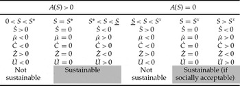
For any current level of pollution S < S*, the stock of pollution must grow along the optimal trajectory. As a consequence, the overall period marginal damage cost of pollution increases. Moreover, the absolute value of the shadow price μ increases. Since the latter is negative, it follows  Given the findings in equation (13), this implies that, in the case of S < S*, consumption must decline over time and gradually more resources must be allocated to pollution abatement activities,
 and
 . This is necessary to slow down the further accumulation of pollution and stop this process in the long run at the optimal level S*. Altogether, this implies a decline of social welfare U(C,S) along the optimal time path, since according to equation (1)
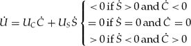
given UC > 0 and US < 0.
The same logic with the opposite signs is valid for the upper branch of the stable trajectory leading towards S* that is, for pollution levels within the interval (S*, S). In this case, the stock of pollution declines and consumption can grow along the optimal time path. As a consequence, social welfare increases over time. In contrast, all variables would remain constant in the steady state which is characterized by S* in table 1.
Dynamic properties on the optimal pollution control trajectories
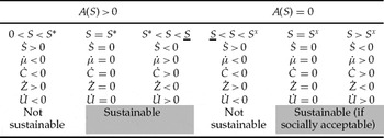
For the two branches of the intertemporal trajectory leading towards Sx, we get exactly the same results (see table 1), presuming that the steady state in (Sx,μx) exists. This requires that the social discount rate is not too small, and that the marginal damage cost of pollution is not too high.
On the whole, table 1 shows that the development for relatively small initial stocks of pollution, that is on the lower branches of the two stable trajectories in figure 2, is not sustainable at all – neither from an environmental nor economic point of view, since pollution must increase and consumption decline over time in order to satisfy the requirements of intertemporal efficiency and to avoid wasteful uses of scarce resources. In contrast, development is sustainable along the optimal trajectory for an initial stock of pollution S > S* and a working assimilative capacity A(S) > 0. In this case, development is environmentally sustainable since the stock of pollution declines along the optimal trajectory and the critical level S is not exceeded. Moreover, it is economically sustainable because consumption grows in line with the above process. The same conclusion can be drawn for initial levels of pollution S > Sx, if the steady state at Sx exists and if the existence of a totally destroyed assimilative capacity, A(S) = 0, is accepted for sustainability from a societal and ethical point of view.
This is a normative question that cannot be answered on purely analytical grounds, but requires a social discourse and an expression of values that are not necessarily captured in our welfare function. In contrast, if S constitutes a critical level of pollution that must not be exceeded at any time, then an accumulation of pollution above this level would be non-sustainable by definition. In this case, a minimum condition for sustainable development would require moving above the critical level of environmental quality (cf. Hediger, Reference Hediger1999) and reducing the stock of pollution below S in a cost-effective way.Footnote 8
For problems with a strictly increasing assimilation function, such as represented by cases (i) and (ii) in figure 1, only one saddle point exists (cf. Cesar and de Zeeuw, Reference Cesar, de Zeeuw, Carraro and Filar1995). Consequently, the above analysis reduces to the two branches of the optimal trajectory leading to the long-term optimum with S*. For initial levels of pollution below this steady-state level (S < S*), the development along the optimal trajectory is not sustainable. In contrast, for pollution levels above the long-term optimum (S > S*), an adjustment process towards this steady state is required which is both environmentally and economically sustainable.
4. Optimal pollution control with capital accumulation
The analysis in the previous section reveals that we must distinguish two different types of the pollution control problem: (a) one with further optimal pollutant accumulation and (b) one of environmental restoration with a net reduction of pollution. Moreover, it shows that the existence of a constant productive capacity is not in general sufficient for sustainable development. Rather, an important case exists where intertemporal efficiency requires the sacrifice of consumption and the allocation of an increasing amount of output to pollution abatement, while the stock of pollution is allowed to further increase along the optimal trajectory. In this case, investments are required to further enhance the economy's production capacity and to compensate for environmental damage. Therefore, we relax the assumption of a fixed production capacity and replace equation (2) by

with YK > 0, YKK < 0 and 
In this case, the total output Y is produced with man-made capital K and a constant input of labour L. Total output Y is allocated to consumption C, pollution abatement Z and investment I in the stock of man-made capital K. The latter consists of both physical assets and knowledge, and depreciates at a constant proportionate rate δ:

This results in an expanded optimization problem with two state variables that is represented by the following current-value Hamiltonian with the additional costate variable ϕ representing the shadow price of capital:

Using the first-order optimality conditions, we get the subsequent set of equations that determine the long-term welfare maximizing trajectory for given initial stocks of capital and pollution, K 0 and S 0, respectively:



Using equations (1) and (18) and taking into consideration that E′ > 0 and E′ > 0, we get

Thus, whether it would be optimal for consumption to grow depends on the relationship between the optimal trajectories of the shadow prices and the marginal rate of emissions, i.e., on whether  is positive or not. According to (20), the first term is a function of the capital stock K and of the discount and depreciation rates ρ and δ. Thus, it is

The implicit price of capital must increase, if the marginal productivity of capital YK is below the long-term optimum ρ + δ. This implies that the capital stock and thus total output must shrink along the optimal trajectory  , which is the case for initial capital endowment K 0 > K*.
In contrast,  is negative and the capital stock must grow if YK is larger than ρ + δ. In other words, for an initial stock of capital below the steady-state level (K 0 < K*), the capital stock must increase
 and the adjoint shadow price decline
 .
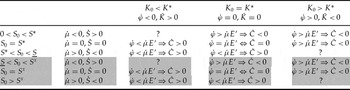
As shown in the previous section, the shadow price of pollution increases according to equation (19) with the accumulation of pollution and declines if the stock of pollution decreases along the optimal trajectory. In table 2, this information on  and
 is combined with the above results about the relationship between and
 . It shows the same pattern for the domain with intact assimilative capacity, A(S) > 0 (i.e., for 0 < S < S), and the one where this ecosystem function is fully destroyed (A(S) = 0, i.e., for S > S).
Optimal development of consumption for different levels of pollution and capital
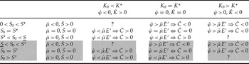
Given the relationship between and , on the one hand, and between and , on the other, table 2 indicates that along the optimal trajectory consumption should grow for low initial levels of capital (K 0 < K*) and high levels of pollution (S* < S 0 < S and S 0 > Sx, respectively). In contrast, consumption should decline if the initial level of capital is above the long-term optimum but pollution below the steady-state level S* and between S and Sx, respectively. The economy is obviously in a steady state if  , which is the case in the long-term optimum (S*, K*).
To further investigate the optimal trajectories for economic development, we employ equations (20) and (21) and get the modified condition for economic growth
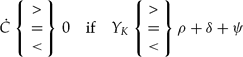
with

Since E′ > 0 and ϕ > 0, it follows furthermore that

Thus, ψ is positive for low initial pollution and capital endowment (0 < S 0 < S* and 0 < K 0 < K*). This implies that the equality condition YK = ρ + δ +ψ > ρ + δ which determines that the limit for optimal consumption growth is higher than the standard Ramsey rule (without pollution) would suggest. Given the declining marginal productivity of capital, it further follows that the steady-state level of capital K*, where YK(K*, L) = ρ + δ +ψ, is below the reference level K° for the case without pollution, where YK(K°, L) = ρ + δ. This conclusion can also be drawn for the initial situation with S* < S 0 < S and K 0 > K*, where ψ < 0 and therefore YK(K*, L) = ρ + δ + ψ < ρ + δ = YK(K°, L).Footnote 9 Thus, when taking welfare losses due to pollutant accumulation into account, we get a lower equilibrium stock of capital (K* < K°), below which the economy (consumption and capital) would optimally grow, and above which it would have to shrink along the optimal trajectory.
However, as table 2 indicates, the solution is ambiguous for the fields that show a question mark because the sign of is not clearly determined. For a further analysis, we define

This allows us to represent K as an inverse function of its marginal productivity YK

Under consideration of equations (23) and (24), it follows

This implies that – in contrast to the optimal control problem with a fixed production capacity – consumption growth can be optimal on the lower branch of the stable trajectory leading to S* (see figure 2) for small initial capital stocks K 0 < g −1(ρ + δ + ψ). This is feasible as long as more additional output is generated from the growing capital stock than the economy must use for enhancing pollution abatement and for investment production capital.Footnote 10 Thus, a further accumulation of pollution can be sustainable
(a) in the sense of ‘very weak sustainability’ if consumption grows along the optimal trajectory, that is, if
 and
(b) in the sense of ‘weak sustainability’ if consumption growth is sufficiently large to compensate for the pollution-induced welfare loss, that is if
.Footnote 11
 and
 .
However, consumption must decline along the optimal trajectory with further pollutant accumulation, as in the case of Section 3, as long as the capital stock exceeds the critical level K = g −1(ρ + δ + ψ). In principle, this could change along the optimal trajectory. Hence, in the case with low capital endowment, consumption growth could be optimal in an initial phase of development and then have to decline in a later phase. This is exclusively driven by efficiency criteria that are necessary for net present value maximization of social welfare.
In short, the development of a growing economy which expands its productive capacity through physical and knowledge capital accumulation can be sustainable from both an economic and social welfare perspective, even in a situation with further pollution accumulation. However, to compensate the growing disutility of pollution, the rate of capital accumulation must be higher if society wants to achieve a welfare improving path of weak sustainability, than a simple criterion of economic sustainability (measured in terms of rising consumption) would suggest. For a wealthy economy with a relatively high stock of man-made capital (physical assets and knowledge) which faces a problem of continued pollution accumulation, such as the enhanced greenhouse effect, the above results indicate that a further accumulation of capital according to the Ramsey rule might not be sufficient for sustainable development. Higher rates of investment might be required to maintain a constant flow of welfare in this case. This links our analysis to that of sustainable development with natural resources and the investment of rents into reproducible capital.
5. Pollution, sustainability and the investment of environmental rents
The investment of resource rents has originally been proposed by Solow (Reference Solow1974) and Hartwick (Reference Hartwick1977) as an approach of intergenerational equity for an economy that exploits a stock on non-renewable resources. Yet, our analysis in section 2 shows that maintenance of an economy's aggregate production capacity will not in general be sufficient to sustain a constant level of consumption in the presence of pollution accumulation, to say nothing of non-declining social welfare. However, it is straightforward to think about a Hartwick-type investment rule of earmarking the ecological rents that accrue from using nature's assimilative capacity to foster the accumulation of man-made capital. For our intertemporal allocation problem that is represented by the Hamiltonian in equation (17), the corresponding investment rule is given by

This results in a constant value of total capital. Consequently, the value of the Hamiltonian is equal to the instantaneous value of social welfare:  .Footnote 12
Using the total derivative of equation (17) with respect to time and the optimality conditions (18)–(20), it turns out that the investment of the environmental rents according to equation (29) enables a constant flow of social welfare. It is

and thus

As a consequence, the value of social welfare

is the same for all points on the trajectory leading to the long-term optimum stock of pollution S*, as long as the rents accruing from using nature's assimilative capacity are invested into reproducible capital. This is the maximum sustainable value of welfare that can be achieved, given the initial stocks of capital and pollution K 0 and S 0.
For the important problem with S 0 < S*, this implies a lower level of consumption than the result of the pure pollution control problem would suggest. Consumers are requested to sacrifice some instantaneous benefits in order to maintain a constant level of welfare over time. However, they receive a return in the long run in form of higher welfare and consumption.
The net present value of the maximum constant welfare stream is equal to the traditional net present value of social welfare without investment of the environmental rents

Moreover, the optimal time path of pollution accumulation and the related shadow price are exactly the same in both cases. The difference between the two cases is only the level of instantaneous consumption and welfare. Hence, the selection of one or the other alternative is a matter of societal preferences for long-term versus short-term benefits.
In analogy to Chichilnisky's (Reference Chichilnisky1996, Reference Chichilnisky1997) definition of sustainable preferences, this selection problem can formally be expressed in present value terms as a weighted sum of the pure net present value of welfare maximization and the largest permanently maintainable and therefore intergenerationally equitable level of social welfare

In the extreme case with θ = 1, priority is given to the immediate but non-sustainable benefits of present consumption. In the other extreme with θ = 0, a constant and sustainable flow of welfare and thus the long run is prioritized. The latter case requires the investment of the environmental rents accruing from nature's pollution assimilation. All other cases (0 < θ < 1) imply a compromise between preference given to the present and the future. However, all cases are equivalent with regard to the intertemporal efficiency, since they all imply the same trajectory of pollution accumulation for a given initial state.
Hence, the optimal trajectory with an initial stock of pollution S 0 < S* is sustainable in the conventional sense of maintaining the maximum constant flow of welfare if the environmental rents are invested into any form of man-made capital that enhances the economy's productive capacity. It is sustainable with respect to the Chichilnisky criterion, if the society finds a balance between the two extremes of pure net present value maximization and the maintenance of a constant welfare level, whereas the normative choice of the weighting factor θ is crucial.
For an initial stock of pollution S 0 > S* but S 0 < S, the investment guideline (29) should not be applied as a rule, because the optimal trajectory is generally characterized by an increase in environmental quality  and instantaneous consumption
 , or at least in social welfare
 .Footnote 13 One exception, however, could be the restoration of water quality in a eutrophicated lake or the restoration of a contaminated soil that requires costly investments in the beginning, irrespective of whether S 0 < S or S 0 > S. In both cases, a Hartwick-type rule could be used to make the polluters paying a fee equivalent to the environmental rent and to amortize the related debt that results from an initial investment required for environmental quality improvement in the long run.
6. Conclusion
The control of accumulative pollution in the environment is an important task that must be included in any sustainable development policy. From a welfare economic and efficiency oriented point of view, this will not imply a strong sustainability constraint of a constant or declining stock of pollution, such as propagated by Daly (Reference Daly1991) and investigated by Chevé (Reference Chevé2000). Rather, to avoid wasteful uses of scarce resources, sustainable development requires an efficient resource allocation. This theoretically goes along with the optimal control of accumulative pollutants. As shown in this paper, the latter involves three distinct types of problem that must be differently analysed with regard to the implementation of environmental policy within a sustainable development framework.
The first one is related to the potential long-term optimum (saddle point) that can exist at a level of accumulated pollution where the ecosystem's assimilative capacity is completely destroyed. From a purely efficiency-oriented perspective, it can be optimal to let the stock of pollution further increase if the initial level is already in the domain where the assimilative capacity is zero. From a societal perspective, however, the normative question remains whether it can be desirable to let an ecosystem die, and how the environmental quality could be restored with technological measures. This issue is not specifically investigated in the present paper, and remains subject to further theoretical and applied research.
The second problem area is characterized by a relatively high initial stock of pollution that is above the long-term optimum. In this case – which has also been investigated by Hartwick (Reference Hartwick1997) and Chevé (Reference Chevé2000) – optimal resource allocation results in a decline of the accumulated stock of pollution and consumption growth. Apparently, this does not pose a problem for sustainable development since the optimal trajectory satisfies both criteria of economic and environmental sustainability. Hence, a policy of optimal pollution control will in general contribute to sustainable development in situations with relatively high initial pollution and a working assimilation capacity of the environment. But, it will require a relatively high share of capacity allocated to pollution abatement, which can subsequently decline over time and allow for an increase in the rate of consumption. Yet, this does not imply a recommendation to first overpollute the environment and then to start a sustainable development program, as this would not be compatible with the minimum requirement of intertemporal efficiency and would result in avoidable welfare losses. Rather, an optimal pollution control strategy may avoid such high stocks of pollution. This brings us to the next case of investigation.
The third domain of the optimal pollution control problem is the one that, apart from global problems like the depletion of the ozone layer and the enhanced greenhouse effect, might gain the least attention in the public, since it refers to the situation with a relatively low initial stock of pollution below the long-term optimum and with still low or even neglectable damage costs. But, as shown in this paper, this situation refers to the most important challenge with regard to sustainable development because the optimal pollution control trajectory in this domain generally involves a continued accumulation of pollution and a decline of consumption. This is particularly the case in wealthy economies with a high initial stock of capital. In contrast, poorer economies might have the option of following a trajectory of optimal capital accumulation that generates sufficient additional output to increase anti-pollution efforts and, at the same time, facilitate growth in consumption. Thus, despite continued pollution accumulation, the poor-country case can be sustainable from a weak sustainability perspective of non-declining welfare, whereas the one of the wealthy economy may be environmentally and economically unsustainable. In the latter case, additional investment in man-made capital will be required to achieve a sustainable development path. To this end, the economy might invest the environmental rents accruing from the use of nature's assimilative capacity and increase its total productive capacity which is required for growth in consumption and pollution abatement activities. With the application of such a modified Hartwick-type investment rule, the economy could maintain a constant flow of welfare, even in the case of continued pollution accumulation along an intertemporally optimal trajectory.
The determination of the above rent is a particular research challenge. It requires adequate knowledge of the assimilative capacity and the dynamics of pollution accumulation, and it calls for the solution of the entire optimal control problem in order to provide policy information about the shadow prices of pollution and capital. Without this information, the sustainability of economic development and environmental policy cannot be judged in the presence of continued accumulation of pollution, such as the enhanced greenhouse effect. Moreover, the choice of a particular policy and investment of environmental rents into reproducible capital involves the selection of different levels of instantaneous consumption and welfare. This is a matter of societal preferences for short-term and long-term benefits, respectively. For wealthier economies with a relatively high initial stock of capital, this selection problem can be formally solved with Chichilnisky's sustainability criterion. The latter captures a priority given to immediate but non-sustainable consumption, on one side, a priority for a constant and sustainable flow of welfare, on the other, and a set of mixed cases between these two extremes. In the first case, net present value maximization of social welfare is the decision criterion without investment of resource rents. In the other extreme, the above Hartwick rule must be applied and all environmental rents accruing from nature's assimilative capacity must be invested into man-made capital in order to maintain a constant flow of instantaneous welfare. This would facilitate growth in consumption sufficient to compensate for the rising disutility of pollution. However, the ultimate choice is about the weighting factors between the two extremes, or in other words between traditional net present value maximization and weak sustainability, while the efficient use of scarce resources and thus the need for optimal pollution control is a prerequisite.
Appendix
As illustrated in figure 2, the two long-term optima (S*, μ*) and (Sx, μx) are defined by the intersection of the and demarcation curves. The former can be determined by setting in equation (9)
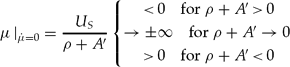
This partial equilibrium locus is zero for S = 0 and has a pole at the pollution level S = S #, where the ‘pollution discount rate’ ρ+A′(S) = 0. Moreover, it is discontinuous at the level S = S where the assimilative capacity is destroyed

For S ≤ S#, the gradient of the curve is strictly negative and, for S# ≤ S ≤ S, it can change sign if 

It is strictly negative for S ≥ S
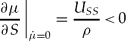
The demarcation curve is determined by including the partial stationary-state condition f(C) = A(S) in equation (10). If the function f is invertible, it follows C = f −1(A(S)) and thus

From this, we get
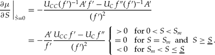
The shape of the curve is characterized by the A(S) curve. Starting with S = 0 in the point
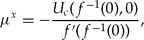
the conditional shadow price  increases for low levels of pollution, reaches the maximum at S = Sm, declines afterwards and remains constant for very high levels of pollution where the assimilative capacity is destroyed.
The dynamics of state and costate variables are caused by any deviation from the and isoclines. For different conditions, the direction of the resulting adjustment processes is depicted by the arrows in figure 2. Their orientation can be determined on the basis of economic reasoning, taking −μ as price charged on pollutant emissions. For each point above the curve, the incentive from the hypothetical effluent charge −μ would not be sufficient to maintain a constant level of pollution. The latter would increase, which is indicated by arrows pointing to the right. The opposite is the case for any point below the curve.
To determine the orientation of the adjustment process from points deviating from the locus, we consider equations (9) and (A1), and get

Considering the discontinuity of the curve, we must distinguish three cases:
(a) A > 0 and ρ + A′ > 0, i.e., 0 < S < S #
For points below the
locus – i.e., – we get . This is indicated by the downward pointing arrows in figure 2. The opposite applies for points above the curve.(b) A > 0 and ρ + A′ < 0, i.e., S # < S < S
The orientation of the arrows changes because ρ + A′ is negative.
(c) A = 0, A′ = 0 and ρ > 0, i.e., S > S
The same logic applies as for case (a) after replacing ρ + A′ by ρ.
 – we get
 . This is indicated by the downward pointing arrows in
Additional remarks
• The solution is ambiguous in S due to the discontinuity of A(S).
• The optimal trajectory for S > Sx only exists if E(C) < G(Z), i.e., if a substantial part of the economy's productive capacity is devoted to pollution abatement and cleaning activities Z, and therefore not available for consumption.