1. Introduction
Humanoid robots possess high dexterity, making them valuable in various applications such as navigating cluttered environments, handling objects, and even folding clothes. Research efforts have extensively focused on refining the capabilities of these robots, especially in tasks such as object manipulation in cluttered environments. Kuffner et al. [Reference Kuffner, Kagami, Nishiwaki, Inaba and Inoue1] introduced a sampling-based method that utilizes Rapidly exploring random trees (RRTs) to plan dynamically stable and collision-free trajectories for reaching an object by a humanoid robot. By employing “AutoBalancer,” a dynamics filter function, this approach efficiently generates a final trajectory that ensures both dynamic stability and collision avoidance. Dalibard et al. [Reference Dalibard, Nakhaei, Lamiraux and Laumond2] explored the use of RRTs to create collision-free paths, which were then optimized to achieve dynamic stability and natural, human-like motion in humanoids during for variety of applications like reaching an object. Teja et al. [Reference Teja, James and Shah3] divided the humanoid into two sub-chains, utilizing RRT* to generate a statically stable and collision-free optimal path for one sub-chain while computing joint positions for the other using inverse kinematics. An extension to the bilateral Fast Marching Trees in the form of waypoints is used in Balachandran et al. [Reference K., Balachandran and Shah4] for whole-body motion planning of humanoid robots. The goal configuration in the above method is determined by gradient-based inverse kinematics coupled with the optimization process. The upper body motion of a humanoid robot is generated in Ruchanurucks [Reference Ruchanurucks5] using B-splines based functions and limits over various physical attributes like joint limit, torque limit, and collisions are set by appropriate coefficients of the B-splines. A smooth interpolation method of the variable-time interval is proposed in Yu et al. [Reference Yu, Zhou and Huang6] to generate the collision-free and energy-jerk-minimal trajectory by using quintic B-spline curve and normal distribution.
Utilizing the redundancy present in redundant robots through the application of the Jacobian’s null space projection facilitates task decomposition, enabling the allocation of distinct subtasks to the robots. The concept of task priority was introduced in Nakamura et al. [Reference Nakamura, Hanafusa and Yoshikawa7], where a required task is divided into subtasks according to the order of priority. By employing pseudoinverses of Jacobian matrices, the joint rates of the robot manipulator are determined, enabling the execution of lower-priority subtasks using redundancy without compromising the higher-priority subtasks. Ott et al. [Reference Ott, Dietrich and Albu-Schäffer8] harnessed redundancy for dynamic control in the seven degree of freedoms (DoFs) compliant arm of the humanoid robot Justin, employing null-space projection techniques to handle multiple prioritized tasks. Gams et al. [Reference Gams, Van den Kieboom, Dzeladini, Ude and Ijspeert9] utilize task decomposition for real-time full body motion imitation on COMAN robot where the primary task is set as maintaining the dynamic balance based on ZMP criteria, and the secondary task is set as motion imitation. Karimi and Ahmadi [Reference Karimi and Ahmadi10] focus on implementing strict task priority allocation for kinematic control and obstacle avoidance on a five DoFs planar manipulator and on a seven DoFs biped robot. An adaptive weighted Newton iteration is used in Liu et al. [Reference Liu, Huang, Liu, Guo, Wang and Tan11] for energy efficient trajectory considering the kinematic constraints on a 6 DoFs manipulator. The task decomposition method is used in Tomic et al. [Reference Tomić, Chevallereau, Jovanović, Potkonjak and Rodić12] for generating human-like motion on robot ROMEO by imitating the motion in Cartesian and joint spaces, obtained from the imitation algorithm. Quan et el. [Reference Quan, Wang, Zhao, Lv, Zhao and Lv13] utilized the idea of redundancy angle discretization on a seven DoFs modular manipulator and proposed the concept of the self-motion space of the trajectory to obtain collision-free solutions for a fixed Cartesian trajectory. An optimal collision-free trajectory for redundant manipulators considering higher mechanical advantage was achieved in Zacharia and Xidias [Reference Zacharia and Xidias14] by setting an optimal sequence of the subtasks: cycle time, collision avoidance, and the manipulability index using Genetic Algorithm coupled with the Bump-Surface concept.
Zhao and Wei [Reference Zhao and Wei15] used the gradient projection of the hierarchical planning strategy into the null-space of Jacobian to generate human-like motion of the joint trajectory in seven DoFs Robai robotic arm in reaching and grasping of object. A framework for controlling the acceleration in Cartesian space to manage the execution of operational tasks and constraints for human-like motion on Honda humanoid robot model was introduced in Hammam et al. [Reference Hammam, Wensing, Dariush and Orin16] by incorporating a dynamically consistent redundancy resolution method to minimize joint motions. A multi-priority control approach for asymmetric coordination in redundant dual arm was introduced in Zhang et al. [Reference Zhang, Qu, Liu and Fu17] by dividing the control into the main task and the secondary task. The main task control involves regulating the errors of the two end effectors and their relative errors by constructing a model of spatial parallel spring and damping, which establishes the dual-arm coordination impedance relationship in Cartesian space. The secondary task control focuses on optimizing the performance of redundant joint impedance and avoiding joint limits in the null space. Jeong and Chang [Reference Jeong and Chang18] apply the Lagrangian multiplier method to address the task-priority challenge in a 28 DoFs humanoid robot, using the square error of the end-effector acceleration as the criterion function. The subtasks are arranged in decreasing priority order, encompassing joint limit, static balance, left foot position, and the motion of a fencing sword striking a target. This approach enables the precise execution of the fencing sword subtask.
Tsuichihara et al. [Reference Tsuichihara, Hakamata, Ricardez, Takamatsu and Ogasawara19] solve inverse kinematics of humanoid robot HRP-4 for the task of reaching low-height positions by both hands in real time. The orientation of the torso was calculated using a regressor and then obtained final position of the center of mass (CoM) for a given target configuration. In each control step, the author first computes the joint angles of the lower body from the CoM position, feet position, and torso orientation, and then the joint angles of both arms. Sentis and Khatib [Reference Sentis and Khatib20] use redundancy resolution for task prioritization to establish a hierarchy between a set of tasks by giving the highest priority to constraint-handling tasks such as balance control, joint limit, and collision avoidance, while projecting operational tasks such as hand control and foot control in the null space and then controlling the posture with the available redundancy. Task priority is used in Acar and Murakami [Reference Acar and Murakami21] for the control task of dynamic balance and end effector of a two-wheeled mobile manipulator. The problem of balance of humanoid robots during object handling while standing is tackled in Tsuichihara et al. [Reference Tsuichihara, Yamaguchi, Takamatsu and Ogasawara22] using the weighted pseudo-inverse of Jacobian. The work in Sugiura et al. [Reference Sugiura, Gienger, JANßEN and Goerick23] addresses the self-collision problem in real time by applying a virtual force in the direction of collision and also by using a dynamic task prioritizing method that effectively combines prioritization for reaching a target and avoiding collisions.
Hip and end-effector trajectory.

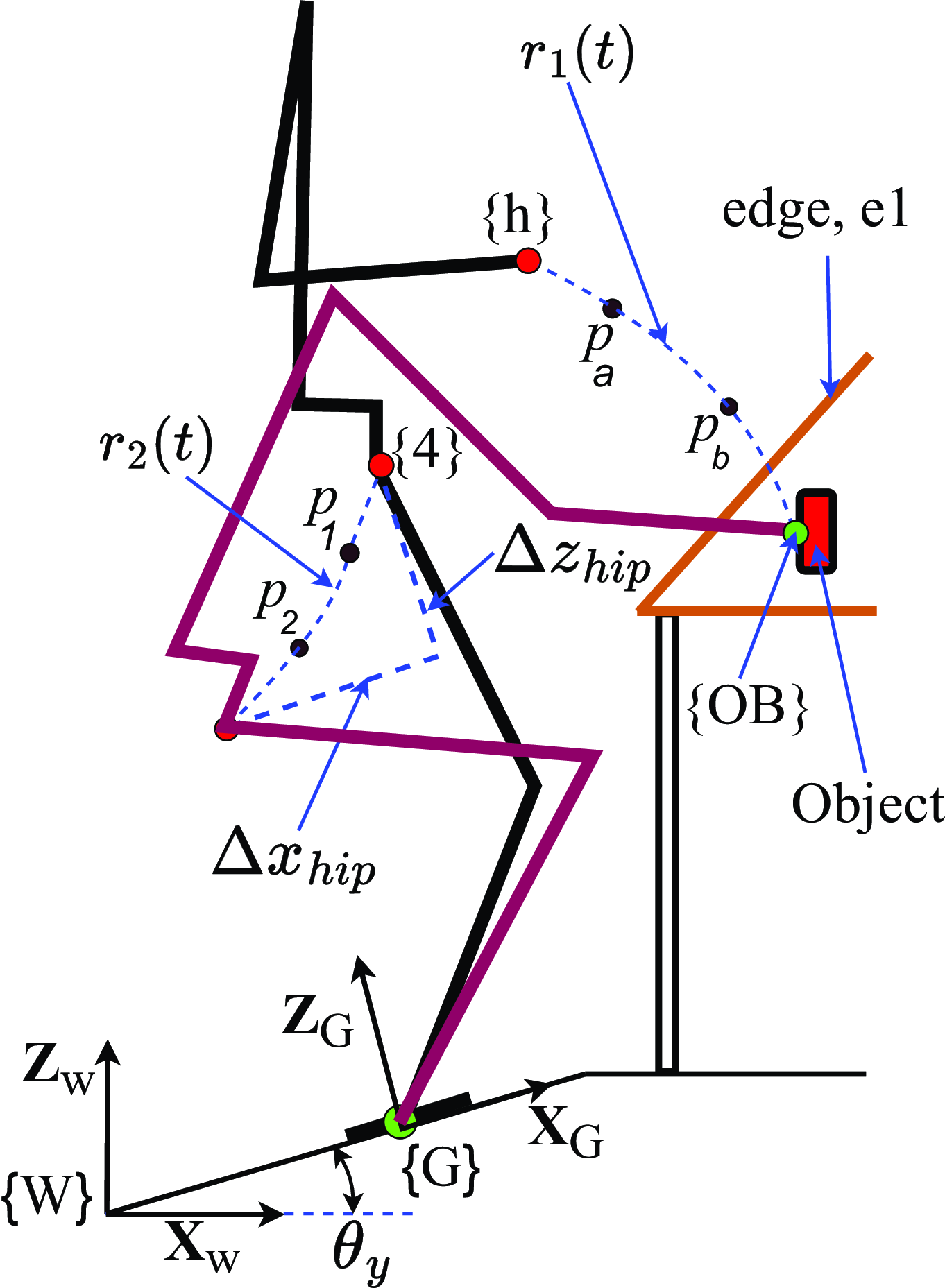
The existing work in humanoid robots fails to address the energy expenditure of humanoid robots during pick and place. This paper focused on finding the minimum number of subtasks and determining energy optimal trajectory by considering the dynamics of the whole body robot without compromising the dynamic balance and end-effector manipulability during pick and place application from table to floor. The motion of humanoid robots is highly complex due to the branched chain and redundancy present. To reduce this complexity and also to solve the energy-optimal problem simpler, the Jacobian method of task decomposition/redundancy resolution is used in our work. Setting too many subtasks increases the complexity of the problem and conflict between the subtasks arises. Setting a lesser number of subtasks might reduce the complexity, but it will not be able to fulfill our main goal. Our work deals with the three distinct task decomposition of whole-body humanoid robots to find energy-optimal, dynamically balanced, and obstacle-free trajectories for pick-and-place applications. The whole task of pick and place is divided into three stages stage I (approach), stage II (pick), and stage III (place). Each stage is solved using the method of Pseudoinverse of Jacobian matrix for redundancy resolution on task priority basis where the various constants are optimized using PSO. The end effector of the robot, i.e., the task hand tracking a desired trajectory,
 $\boldsymbol {r}_1(t)$
is considered as primary task
 $\mathcal {T}_1$
, and the hip of the robot, i.e., origin of frame
 $\{4\}$
tracking a desired trajectory
 $\boldsymbol {r}_2(t)$
is chosen as secondary task
 $\mathcal {T}_2$
as shown in Figure 1 and maximizing the manipulability of the robot as tertiary task
 $\mathcal {T}_3$
. Task
 $\mathcal {T}_1$
is of the highest priority, followed by task
 $\mathcal {T}_2$
and task
 $\mathcal {T}_3$
has the least priority. Newton–Euler (NE) for tree type robot is used to solve the dynamics of the humanoid robot. The main contribution of this paper is finding an energy-optimal, obstacle-free, and dynamically balanced whole-body trajectory and also maximizing the manipulability
 $V(\boldsymbol {q})$
Kang et al. [Reference Kang, Meng and Xu24] of the end effector as the robot moves along the desired trajectory. The optimal number of subtasks to be set during pick and place application is discussed in Sections 5.2, 5.3, and 5.4. The structure of the paper is as outlined below: Section 2 details the methodology for generating desired trajectories, Section 3 discusses the dynamics of tree-type robotic system, and Section 4 presents the generation of trajectories that are energy optimal, obstacle-free, and dynamically balanced using PSO. The simulation and results are presented in Section 5, while Section 6 concludes the paper.
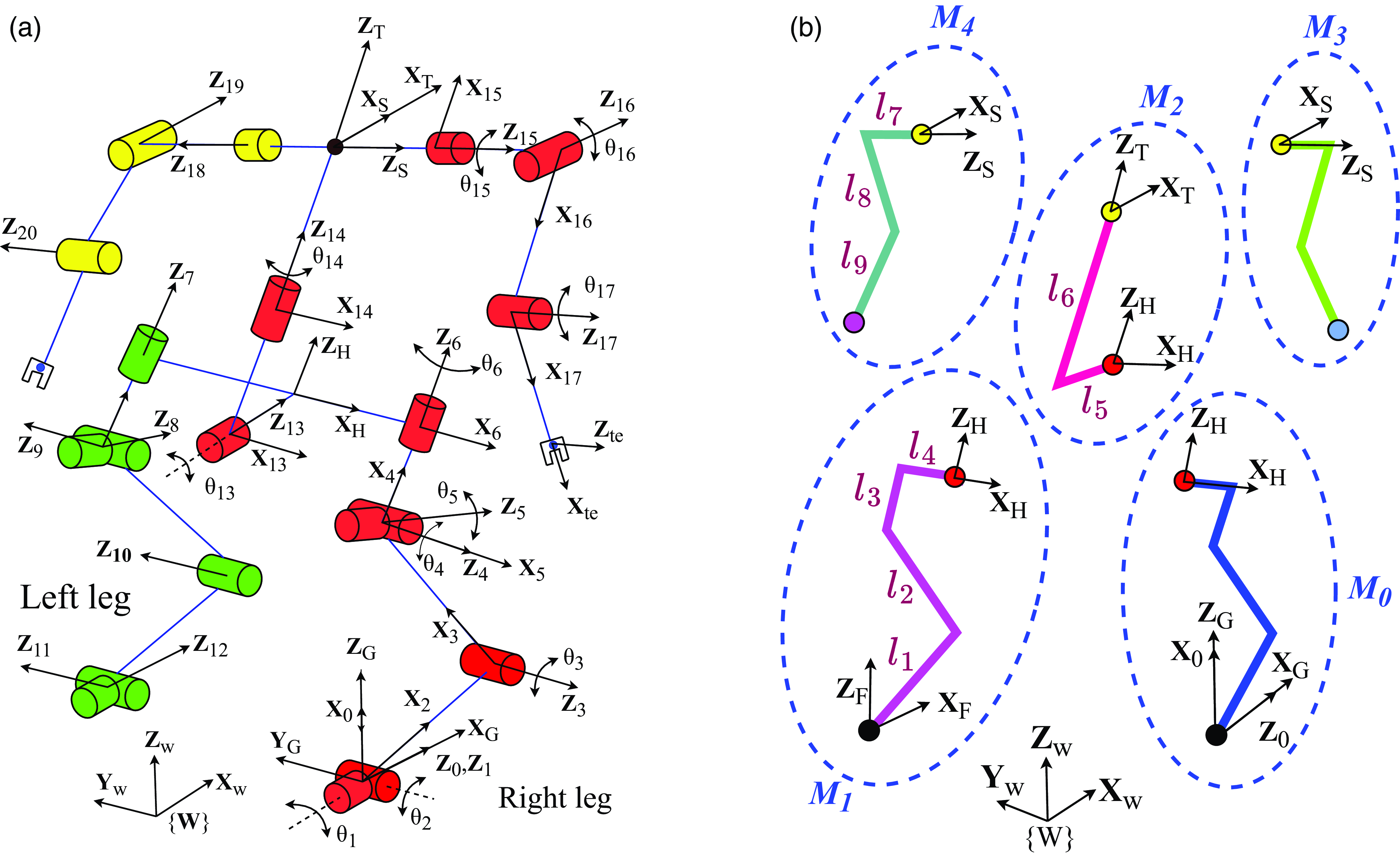
(a) 20 degrees of freedom kinematic model. (b) Modules architecture of the full-body humanoid.

2. Methodology
The kinematic model of the full-body humanoid is shown in Figure 2a. The whole body is divided into three sub-chains: primary chain, secondary chain, and tertiary chain. The right leg, torso, and right hand form the primary chain, the left leg forms the secondary chain, and the left-hand forms the tertiary chain. The joints associated with the frames
 $\{1\}$
,
 $\{5\}$
, and
 $\{6\}$
of the primary chain and that of the frame
 $\{7\}$
,
 $\{8\}$
, and
 $\{12\}$
of the secondary chain are locked to make the hip motion planer. So, the primary chain has only eight active joints. The joint rates of the primary chain are computed using the pseudoinverse method Eq. (3) and that of the secondary chain is calculated using the geometrical method of inverse kinematics at each time step. All the joints of the tertiary chain are also locked while performing the task. The tree-type robotic system is also divided into 5 different modules as shown in Figure 2b. Frame
 $\{G\}$
is attached to the base of module 0,
 $M_0$
, and Frame
 $\{F\}$
is attached to the end of module 1,
 $M_1$
.
The location and orientation of the humanoid robot are defined by
-
• The location and orientation of the ground frame
 $\{G\}$
with respect to the world frame
$\{W\}$
denoted by
${}^{W}\!\boldsymbol {P}_G \in \mathbb {R}^3$
and
${}^{W}\!\boldsymbol {\Theta }_G \in \mathbb {R}^3$
, respectively.
-
• The location and orientation of the frame
$\{F\}$
with respect to the frame
$\{G\}$
denoted by
${}^{G}\!\boldsymbol {P}_F \in \mathbb {R}^3$
and
${}^{G}\!\boldsymbol {\Theta }_F \in \mathbb {R}^3$
respectively.


 $\boldsymbol {r}_1(t) = \begin{bmatrix} x_1(t) & y_1(t) &z_1(t) \end{bmatrix}^T$
and
 $\boldsymbol {r}_2(t) = \begin{bmatrix} x_2(t) & y_2(t) &z_2(t) \end{bmatrix}^T$
are vector-valued functions where the components are composite splines. Three cubic splines are connected at two via points to form the composite spline by ensuring velocity and acceleration continuity.
 $\boldsymbol {p}_a \in \mathbb {R}^3$
,
 $\boldsymbol {p}_b \in \mathbb {R}^3$
are the two via points for
 $\boldsymbol {r}_1(t)$
and
 $\boldsymbol {p}_1 \in \mathbb {R}^3$
,
 $\boldsymbol {p}_2 \in \mathbb {R}^3$
for
 $\boldsymbol {r}_2(t)$
as shown in Figure 1.
 $\Delta {x_{hip}}$
and
 $\Delta {z_{hip}}$
define the hip displacement while performing the whole task . Out of the eight DoFs of the primary chain, task
 $\mathcal {T}_1$
uses a minimum of three DoFs, task
 $\mathcal {T}_2$
uses two DoFs, and the remaining DoFs are used for the task of maximizing the manipulability index
 $V(\boldsymbol {q})$
of the end effector. The algorithm works in an iterative way where the input required for finding the joint rates using the method of Pseudoinverse of the Jacobian matrix is obtained by the best output values from the PSO algorithm. The following assumptions are made:
-
• Initially, the robot is in a statically balanced state.
-
• Body of the robot is aligned with the unit vector
$\hat {\boldsymbol {Z}}_W$
initially. -
• The location of the robot is such that the end effector is able to reach the object at the extreme end of the table without compromising the dynamic balance.
-
• The object is massless, and there is no force of interaction when the robot picks the object.

The task
 $\mathcal {T}_1$
assigned to the end effector (task hand) of the robot is such that the end effector must reach the target (a fixed point) depending on the stage (stage I, stage II, or stage III). As the task
 $\mathcal {T}_2$
assigned to the robot is primarily responsible for maintaining the balance of the robot, the values
 $\Delta {x_{hip}}$
and
 $\Delta {z_{hip}}$
are such that the zero moment point (ZMP) Vukobratovic and Borovac [Reference Vukobratović and Borovac25] of the whole body humanoid always lies inside the foot support polygon. The above analogy and assumptions clearly shows that task
 $\mathcal {T}_1$
will always be fulfilled and
 $\mathcal {T}_1$
will be of higher priority than
 $\mathcal {T}_2$
. The remaining degree of freedom will be used for maximizing the manipulability end effector if possible as the robot fulfills the task
 $\mathcal {T}_1$
and
 $\mathcal {T}_2$
.
The initial and end conditions required for computing
 $\boldsymbol {r}_1(t)$
and
 $\boldsymbol {r}_2(t)$
are mentioned in Eq. (14), Eq. (15) and Eq. (12), Eq. (13), respectively. The values of
 $\boldsymbol {p}_a, \boldsymbol {p}_b, \boldsymbol {p}_1, \boldsymbol {p}_2, \Delta {x}_{hip}$
, and
 $\Delta {z}_{hip}$
are best value output from the PSO algorithm. Joint rates computed using Eq. (3) are such that the robot fulfills the task
 $\mathcal {T}_1$
,
 $\mathcal {T}_2$
, and
 $\mathcal {T}_3$
. The joint rates obtained from Eq. (3) are used to compute the energy consumed in doing the task by solving the dynamics of the whole body robot. Energy-optimal, dynamically balanced, and obstacle-free trajectories are obtained by optimizing using PSO. The fitness function is a function of energy consumed with the constraint of collision penalty and ZMP violation penalty in the optimization algorithm.
The end-effector trajectory
 $\dot {\boldsymbol {r}}_1$
and hip trajectory
 $\dot {\boldsymbol {r}}_2$
relate to the joint rate vector
 $\boldsymbol {\dot {q}}\in \mathbb {R}^8$
by Eq. (1) and Eq. (2)
 \begin{align} \boldsymbol {\dot {r}}_1 &= \boldsymbol {J}_1\boldsymbol {\dot {q}} \end{align}
 \begin{align} \boldsymbol {\dot {r}}_2 &= \boldsymbol {J}_2\boldsymbol {\dot {q}} \end{align}
where,
 \begin{align*} \boldsymbol {\dot {q}} &= \begin{bmatrix}\dot {\theta }_2 & \dot {\theta }_3 & \dot {\theta }_4 & \dot {\theta }_{13} & \dot {\theta }_{14} & \dot {\theta }_{15} & \dot {\theta }_{16} & \dot {\theta }_{17}\end{bmatrix}^T \\ \boldsymbol {\dot {r}}_1 &= \begin{bmatrix} \dot {x}_1(t) & \dot {y}_1(t) & \dot {z}_1(t) \end{bmatrix}^T \\ \boldsymbol {\dot {r}}_2 &= \begin{bmatrix} \dot {x}_2(t) & \dot {y}_2(t) & \dot {z}_2(t) \end{bmatrix}^T. \end{align*}
Here, Jacobian
 $\boldsymbol {J}_1\in \mathbb {R}^{3 \times 8}$
and Jacobian
 $\boldsymbol {J}_2\in \mathbb {R}^{3 \times 8}$
.
 $\boldsymbol {J}_2$
is written as
 $\boldsymbol {J}_2 = [\boldsymbol {J}_{leg}|\boldsymbol {0}]$
, where
 $\boldsymbol {J}_{leg}\in \mathbb {R}^{3 \times 2}$
relates joint rates
 $\dot {\theta _2}$
and
 $\dot {\theta _3}$
with hip velocity. General solution for
 $\boldsymbol {\dot {q}}$
of Eq. (1) and Eq. (2) that performs primary, secondary, and tertiary tasks is given by Eq. (3), Yoshikawa [Reference Yoshikawa26]
 \begin{equation} \boldsymbol {\dot {q}}_d = \boldsymbol {J}_1^{\dagger }\dot {\boldsymbol {r}}_1 + \tilde {\boldsymbol {J}}^{\dagger }_2(\dot {\boldsymbol {r}}_2 - \boldsymbol {J}_2\boldsymbol {J}^{\dagger }_1\dot {\boldsymbol {r}}_1) + (\boldsymbol {I}_8-\boldsymbol {J}_1^{\dagger }\boldsymbol {J}_1-\tilde {\boldsymbol {J}}^{\dagger }_2\tilde {\boldsymbol {J}}_2)\boldsymbol {k} \end{equation}
where,
 $\boldsymbol {\dot {q}}_d$
is the vector of the desired joint rates. The Jacobian matrices are computed as follows Witney [Reference Witney27]
 \begin{align} \boldsymbol {J} &= \begin{bmatrix} \boldsymbol {J}^1 & \boldsymbol {J}^2 &\ldots & \boldsymbol {J}^n \end{bmatrix} \end{align}
where,
 \begin{align} \boldsymbol {J}^i &= \begin{pmatrix} \hat {z}_{i-1} \times \boldsymbol {p}^{i-1}_n \end{pmatrix}. \end{align}
 $\boldsymbol {J}^i \in \mathbb {R}^{3}$
in Eq. (5) is the
 $i^{th}$
column vector of the Jacobian matrix Eq. (4),
 $\hat {z}_{i-1}$
is a unit vector in the direction of
 $z$
axis of
 $(i-1)^{th}$
frame and
 $\boldsymbol {p}^{i-1}_n \in \mathbb {R}^{3}$
is a vector from the origin of
 $(i-1)^{th}$
frame to that
 $i^{th}$
frame. The augmented Jacobian
 $\boldsymbol {\tilde {J}}_2$
in Eq. (3) is given by
 $\tilde {\boldsymbol {J}}_2 = \boldsymbol {J}_2(\boldsymbol {I}_8 - \boldsymbol {J}^{\dagger }_1\boldsymbol {J}_1)$
, where
 $\boldsymbol {J^{\dagger }} = \boldsymbol {J}^T(\boldsymbol {JJ}^T)^{-1}$
is the Moore–Penrose pseudo-inverse of
 $\boldsymbol {J}$
. The vector
 $\boldsymbol {k}$
in Eq. (3) is given by
 \begin{equation} \boldsymbol {k} = \boldsymbol {K}_p\boldsymbol {\xi } \end{equation}
where
 $\boldsymbol {\xi } \in \mathbb {R}^8$
is the manipulability gradient vector given by Eq. (8),
 $\boldsymbol {K}_p \in \mathbb {R}^{8 \times 8}$
is the appropriate diagonal weight matrix Eq. (7), and the diagonal entries are obtained through optimization.
 \begin{align} \boldsymbol {K}_p &= \begin{bmatrix} k_1 & 0 & \ldots & 0\\ 0 & k_2 & \ldots & 0\\ \vdots & \vdots & \ddots & \vdots \\ 0 & 0 &\ldots & k_8 \end{bmatrix} \end{align}
 \begin{align} \boldsymbol {\xi } &= \begin{bmatrix} \xi _1 & \xi _2 &\ldots &\xi _8 \end{bmatrix}^T \end{align}
where
 \begin{align} \xi _l &= \frac {\partial }{\partial q_l} V(\boldsymbol {q}), V(\boldsymbol {q}) = \sqrt {det(\boldsymbol {J}_1\boldsymbol {J}^T_1)}, \text {$l = 1,2,3,\ldots, 8$}, \end{align}
 \begin{align} \xi _l &= \frac {V(\boldsymbol {q})}{2}tr\left ((\boldsymbol {J}\boldsymbol {J}^T)^{-1}\left (\frac {\partial \boldsymbol {J}}{\partial q_l}\boldsymbol {J}^T + \boldsymbol {J}\frac {\partial \boldsymbol {J}^T}{\partial q_l}\right )\right ) \end{align}
 \begin{align} \xi _l &= \frac {1}{2}V(\boldsymbol {q})\sum ^3_{i,j = 1} a_{ij}(J_{1il}J^T_{1j} + J_{1jl}J^T_{1i}) \end{align}
 $V(\boldsymbol {q})$
is the manipulability of the end effector of the primary chain of the robot,
 $a_{ij}$
is the
 $(i,j)^{th}$
element of
 $(\boldsymbol {J}_1\boldsymbol {J}_1^T)^{-1}$
,
 $\boldsymbol {J}_{1i}$
is the
 $i^{th}$
row vector of
 $\boldsymbol {J}_1$
, and
 $\boldsymbol {J}_{1il}$
is the partial differential of
 $\boldsymbol {J}_{1i}$
with respect to
 $q_l$
.
The initial and end conditions for the hip trajectory are given by Eq. (12) and Eq. (13). As there is no hip motion in the frontal plane during the task, the value of
 $\Delta {y}_{hip}$
is zero. Figure 1 shows the hip trajectory and the via points. Initially, the hip is at
 $\boldsymbol {r}_{{hip}_i} = \begin{bmatrix} x_{{hip}_i}& y_{{hip}_i}& z_{{hip}_i}\end{bmatrix}^T$
, where
 $\boldsymbol {r}_{{hip}_i}$
is the initial hip position at the beginning of a stage and
 $t_c$
is the cycle time for each stage.
 \begin{align} \boldsymbol {r}_2(0) &= \boldsymbol {r}_{{hip}_i} \end{align}
 \begin{align} \boldsymbol {r}_2(t_c) &= \boldsymbol {r}_{{hip}_i} + \begin{bmatrix} \Delta \boldsymbol {x}_{hip}& 0& \Delta \boldsymbol {z}_{hip}\end{bmatrix}^T \end{align}
where
 \begin{align*} \boldsymbol {r}_{{hip}_i} &= {}^{W}\!\boldsymbol {R}^T_0 (^W\!\boldsymbol {P}_{4} - ^W\!\boldsymbol {P}_G) \\ \Delta \boldsymbol {x}_{hip} &= \Delta {x}_{hip}\hat {\boldsymbol {X}}_G \\ \Delta \boldsymbol {z}_{hip} &= \Delta {z}_{hip}\hat {\boldsymbol {Z}}_G \end{align*}
The initial and end conditions for the end effector trajectory
 $r_1(t)$
are given by Eq. (14) and Eq. (15)
 \begin{align} \boldsymbol {r}_1(0) &= {}^{W}\!\boldsymbol {R}^T_0(^W\!\boldsymbol {P}_{h} - ^W\!\boldsymbol {P}_{G}) \end{align}
 \begin{align}\boldsymbol {r}_1(t_c) &= {}^{W}\!\boldsymbol {R}^T_0(^W\!\boldsymbol {P}_{OB} - ^W\!\boldsymbol {P}_{G}) \end{align}
where the rotation matrix
 $^W\!\boldsymbol {R}_0$
rotates the frame {W} to frame {0}, and
 $^W\!\boldsymbol {P}_{G}$
is the position vectors of the frames {G} with respect to frame {W}.
 $^W\!\boldsymbol {P}_{4}$
and
 $^W\!\boldsymbol {P}_{h}$
are the position vectors of the hip and the end effector at the beginning of a stage, and
 $^W\!\boldsymbol {P}_{OB}$
is the target location all with respect to the frame {W} see Figure 1.
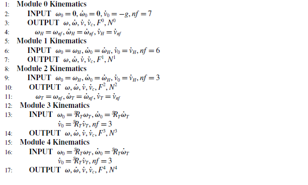
Kinematics for tree type system.

3. Dynamics of tree-type robotic system
A full-body humanoid robot is a tree-type robotic system comprising various modules where each module is a serial chain as shown in Figure 2b. Module
 $M_0$
is the base module of the system, and frame
 $\{\boldsymbol {0}\}$
attached to the module
 $M_0$
is the base of the whole robot. Velocities and accelerations are computed using iterative outward algorithm Craig [Reference Craig28] from the innermost link to the outermost link of each module. For the inter-modular velocity and acceleration propagation, velocities and accelerations available at the end of each module serve as input to the next adjoining module. Algorithm1 shows the kinematics of a tree-type robotic system.
 ${}^{S}\!\boldsymbol {R}_T$
rotates the frame
 $\{T\}$
with respect to frame
 $\{S\}$
. Here,
 $\boldsymbol {\omega }_j$
,
 $\dot {\boldsymbol {\omega }}_j$
, and
 $\dot {\boldsymbol {v}}_j$
are the angular velocity, angular acceleration, and linear acceleration of the origin of frame
 $\{j\}$
, respectively.
 $\dot {\boldsymbol {v}}_{c_j}$
is the acceleration of the center of mass of
 $j^{th}$
link.
 $nf$
is the number of frames in a module excluding the initial base frame of the module required for solving the kinematics and dynamics.
 $\boldsymbol {F}^m$
and
 $\boldsymbol {N}^m$
are read as inertial force vector and inertial torque vector of all the links of module
 $M_m$
where
 $m = 0 \dots 4$
.
Forces and Torques are computed using recursive
 $\textbf {Newton-Euler}$
algorithm (
 $\textbf {NE}$
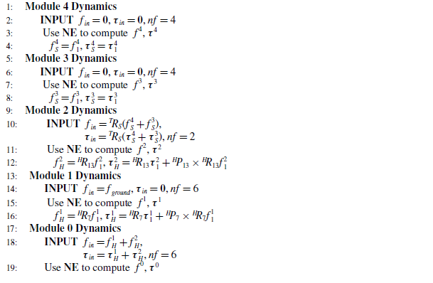
) [Reference Craig28]. The inter-modular force and torque propagation for the tree type is shown in Algorithm2.
 ${}^{H}\!\boldsymbol {R}_{13}$
and
 ${}^{H}\!\boldsymbol {R}_{7}$
are the rotation matrices that rotates the frame
 $\{13\}$
and frame
 $\{7\}$
with respect to frame
 $\{H\}$
respectively.
 ${}^{H}\!\boldsymbol {P}_{13}$
and
 ${}^{H}\!\boldsymbol {P}_{7}$
are the position vectors of the frame
 $\{13\}$
and frame
 $\{7\}$
with respect to frame
 $\{H\}$
, respectively.
 $\boldsymbol {f}^m_j$
and
 $\boldsymbol {\tau }^m_j$
are the net force and net torque on the
 $j^{th}$
link of module
 $M_m$
respectively. Work done (
 $E$
) by the robot for a stage is given by Eq. (16), where
 $t_c$
is the total time taken for a stage.
 $\boldsymbol {\tau }_i(t)$
and
 $\boldsymbol {\dot {\theta }}_i$
are the torque and joint rate for the
 $i^{th}$
link, respectively. The ground reaction force denoted by
 $\boldsymbol {f}_{ground}$
present in line number 14 of the algorithm is taken as half of the weight of the robot.
 \begin{equation} E = \sum _{i=1}^{20}{\int _0^{t_c}} \tau _i(t)\dot {\theta }_i(t)dt \end{equation}
Dynamics for tree type system.

ZMP of the whole robot on inclined plane Sardain and Bessonnet [Reference Sardain and Bessonnet29] is computed by the relation shown in Eq. (17).
 $\boldsymbol {n}$
denotes the unit vector normal to the surface on which the robot stands.
 $\boldsymbol {M}^{g_i}$
and
 $\boldsymbol {F}^{g_i}$
are resultant moment and resultant force respectively, due to the combined effect of gravity and inertia forces.
 \begin{equation} \boldsymbol {P}_{ZMP} = \frac {\boldsymbol {n} \times \boldsymbol {M}^{g_i}}{\boldsymbol {F}^{g_i} \cdot \boldsymbol {n}} \end{equation}
4. Hand and hip trajectory computation using PSO
For every end-effector trajectory
 ${r}_1(t)$
, hip trajectory
 ${r}_2(t)$
and matrix
 $\boldsymbol {K}_p$
, joint rates are computed in such a way the manipulability of the end effector of the robot is maximized. Energy-optimal obstacle-free trajectories are obtained by optimizing using PSO. The input to the optimization algorithm is given by Eq. (18), where
 $\boldsymbol {k}_{opt}$
vector is the diagonal entries of the matrix
 $\boldsymbol {K}_p$
in Eq. (7). Particle Swarm Optimization (PSO) toolbox available in MATLAB is used here for the optimization. The syntax is given by
 $x = particleswarm(fun,nvars,lb,ub)$
, where (fun) is the function to be optimized, (nvars) is the number of variables, (lb) is the lower bound, and (ub) is the upper bound. Here,
 $\boldsymbol {p}_a$
and
 $\boldsymbol {p}_b$
contain three independent variable each. The motion of the hip is confined only in the sagittal plane so
 $\boldsymbol {p}_1$
and
 $\boldsymbol {p}_2$
has two independent variables each. Number of independent variables in
 $\boldsymbol {k}_{opt}$
is discussed in Sections 5.1. Fitness function Eq. (19) required for the optimization algorithm is the sum of work done (
 $E$
) given by Eq. (16) and penalty for constraints violation,
 $\beta$
given by Eq. (20).
 \begin{equation} \boldsymbol {X}_{opt} = \begin{bmatrix} \boldsymbol {p}_a & \boldsymbol {p}_b & \boldsymbol {p}_1 & \boldsymbol {p}_2 &\Delta {x}_{hip} &\Delta {z}_{hip} &\boldsymbol {k}_{opt} \end{bmatrix}^T \end{equation}
 \begin{align} F &= E + \beta \end{align}
 \begin{align} \beta &= \sum _{i=1}^{pn}\beta _i \end{align}
Penalty,
 $\beta$
is imposed during optimization for violating the constraints and
 $pn$
is the number of constraints imposed. Various constraints used here are
-
• ZMP constraints and
-
• collision constraints between the object and robot links.
Virtual surface.

RMS value of the deviation of ZMP of the whole-body humanoid around the point
 $\boldsymbol {P}_{sz}$
located inside the support polygon multiplied by a scalar
 $\gamma _1$
is taken as a penalty. ZMP penalty calculated for the whole instance is shown in Eq. (21) where
 $vp$
is the number of time instances.
 \begin{equation} \beta _1 =\gamma _1 \frac {1}{2}\sqrt {\sum _{i=1}^{vp}\lVert \boldsymbol {P}_{{zmp}_i}- \boldsymbol {P}_{sz}\rVert ^2} \end{equation}
Various penalties are imposed when the robot trajectories interfere with the obstacles. The penalties imposed for obstacle avoidance are divided as penalties for end effector, elbow, shoulder, and neck collision with the edge of the table represented as
 $\beta _2$
,
 $\beta _3$
,
 $\beta _4$
, and
 $\beta _5$
, respectively, and penalties for forearm collision with the edge of the table as
 $\beta _{6}$
. Penalties for end effector, elbow, shoulder, and neck collision with the surface of the table represented as
 $\beta _7$
,
 $\beta _8$
,
 $\beta _9$
, and
 $\beta _{10}$
, respectively, and that of task hand collision with the body of the robot as
 $\beta _{11}$
. Penalties for collision with the edge,
 $e_1$
of the table Figure 1 become effective when the shortest distance
 $d_i$
of the robot part from the edge of the table is less than the threshold distance,
 $d_{min}$
where
 $\gamma _2$
is a scalar Eq. (22).
 $d_{min}$
is introduced in order to avoid the value of
 $\beta _2$
becoming very small when
 $d_2$
approaches zero.
 $d_{min}$
is taken as 10 cm in our work.
 \begin{align} \beta _2 &= \begin{cases} \gamma _2 (d_{min} + d_2),&{\text {if}} \quad d_2 \lt d_{min}\\ {0,}&{\text {otherwise.}} \end{cases} \end{align}
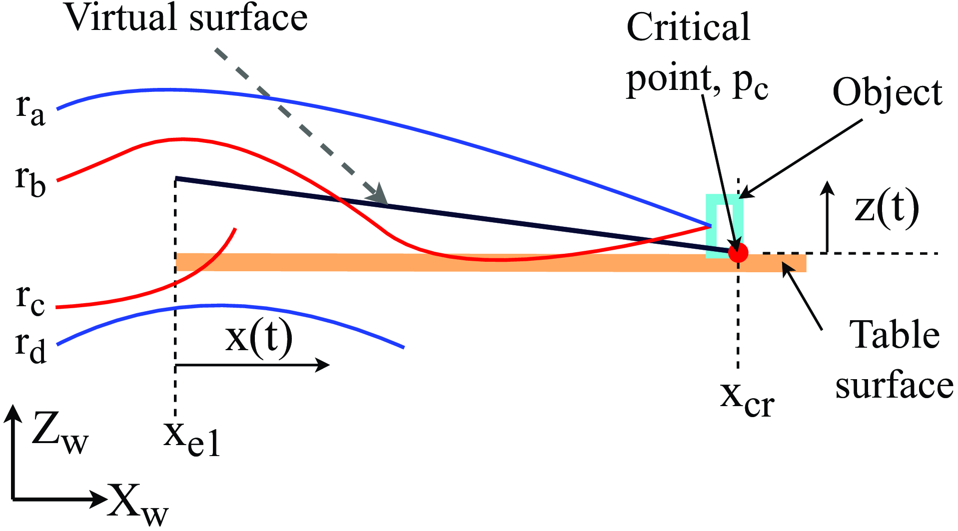
The end-effector trajectory, elbow trajectory, shoulder trajectory, and neck trajectory must not interfere with the surface of the table. For any trajectory
 $r(t) = f(x(t),y(t),z(t))$
, let
 $z_{cross}$
be the set of
 $z(t)$
such that the respective
 $x(t)$
lie in the region (
 $x_{edge},z_{cross}$
) i.e.
 $z_{cross} = \{z(t)|x(t) \in (x_{e1},x_{edge})\}$
. For such a trajectory to be feasible, any element from the set
 $ z_{cross}$
must exclusively lie above the virtual surface created above the table or below the surface of the table. In Figure 3,
 $r_a$
and
 $r_d$
are feasible trajectories, whereas
 $r_b$
and
 $r_c$
are not feasible trajectories. The virtual surface in Figure 3 given by Eq. (23) is created to avoid sliding of the end effector on the table surface or dragging of the object on the table surface. Penalty
 $\beta _{6}$
can be checked by measuring the shortest distance between the forearm and edge,
 $e_1$
of the table Figure 1. Task hand collision with the body of the robot is checked by imposing a constraint on the joint position associated with the frame
 $\{16\}$
and penalty
 $\beta _{11}$
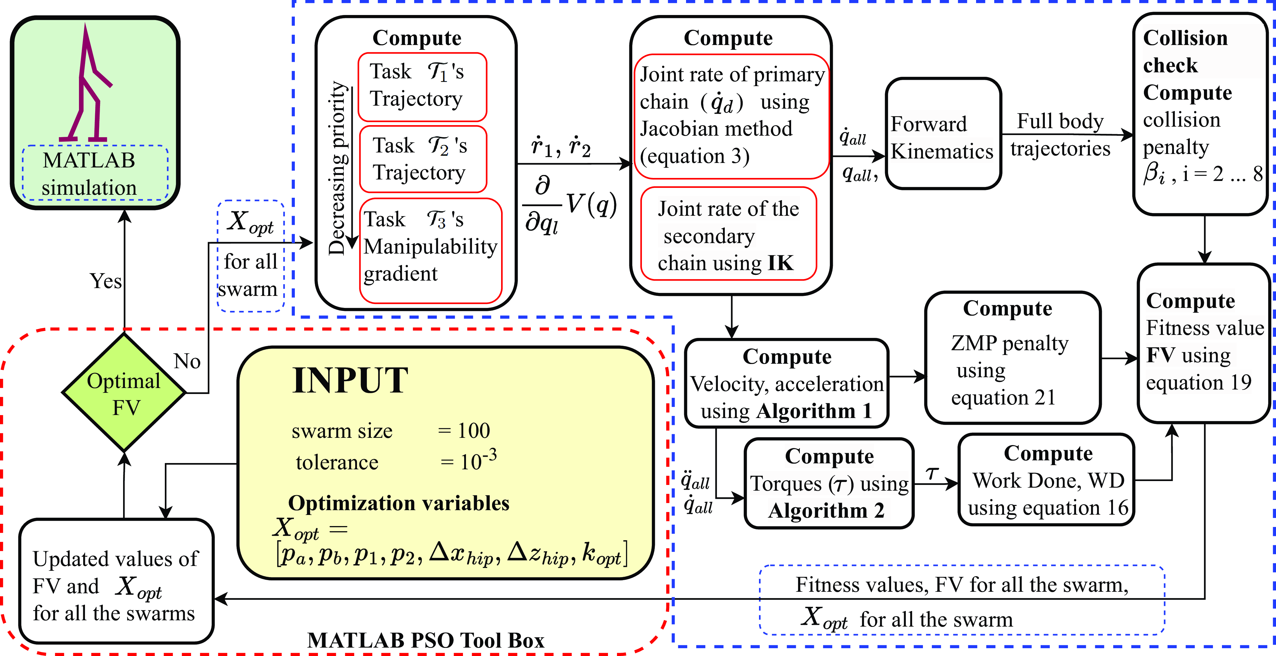
is imposed when the constraint is violated. The complete schematic for finding the energy optimal, obstacle-free, and dynamically balanced full body trajectory that fulfills the primary, secondary, and tertiary task is shown in Figure 4. The algorithm has two parts, PSO part and fitness value generation. It works iteratively until optimal trajectories are achieved. It starts with the initial output from the PSO algorithm where the output will be used to generate the fitness value. The vector
 $\boldsymbol {X}_{{opt}}$
contains the variable of the optimization of swarm size 100, and a tolerance value of
 $10^{-3}$
is used for the optimization. The output from the PSO part is used to generate the desired trajectories for the swarm that fulfill all three subtasks. Work done and ZMP are further computed using the dynamics of the tree-type robotic system. Fitness values are computed using Eq. (19). The vector
 $\boldsymbol {X}_{{opt}}$
along with the generated fitness values for all the swarms are further fed to the PSO part for improving the solution and the iteration goes on until energy optimal, collision-free, and dynamic balanced trajectories are obtained.
 \begin{equation} z(x) = \left ( \frac {x_{cr} - x(t)}{x_{cr}-x_{e1}} \right ) \end{equation}
Schematic for generating the energy-optimal, collision-free, and dynamically balanced trajectory for the full-body humanoid robot that fulfills all the primary, secondary, and tertiary tasks.

5. Simulation and results
The simulation of the robot was conducted in MATLAB R2022b on a
 $12^{th}$
Gen Intel(R) Core(TM) i7-12700 2.10 GHz 16.0 GB RAM Window 11 pro machine. The cycle time
 $t_c$
for each stage is 2 s. The optimization was done using the PSO toolbox available in MATLAB and was run for a swarm size of 100 and function tolerance of
 $10^{-3}$
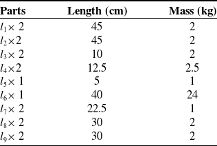
. The length and mass of the different parts of the robot are shown in Table I. Each foot has a mass of 1 kg, length 30 cm, and breadth 12 cm, and the total mass of the robot is 54 kg.
5.1. The value of
$\boldsymbol {k}_{opt}$

For three subtasks decomposition case as in Section 5.2, after assigning the subtask
 $\mathcal {T}_1$
and
 $\mathcal {T}_2$
, three DoFs still remains in the null-space. These extra DoFs are used for maximizing the manipulability
 $V(\boldsymbol {q})$
. Finding an appropriate value of the vector
 $\boldsymbol {k}_{opt}$
as mentioned in Section 4 is the key to determining an energy optimal body configuration. The components of the vector
 $\boldsymbol {k}_{opt}$
is modified as
 $\boldsymbol {k}_{opt} = \begin{bmatrix} 1 & 1 & k_3 & k_4 & k_5 & k_6 & k_7 & k_8\end{bmatrix}^T$
. The intuition behind this is, gradient of
 $V(\boldsymbol {q})$
for
 $q = \theta _2$
and
 $q = \theta _3$
do not contribute in the manipulability maximization. So, the vector
 $\boldsymbol {k}$
in Eq. (6) is written as
 $\boldsymbol {k} = \begin{bmatrix} \xi _1 & \xi _2 & \xi _3k_3 & \xi _4k_4 & \xi _5k_5 & \xi _6k_6 & \xi _7k_7 & \xi _8k_8\end{bmatrix}^T$
.
Length and mass of parts of the robot. Figure 2b shows the meaning of each symbols.

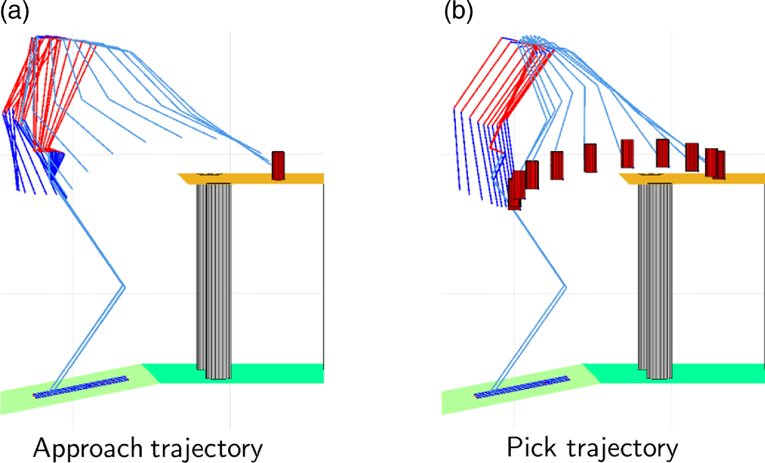
Trajectories for
 $\boldsymbol {k}_{opt} = \begin{bmatrix} 1 & 1 & k_3 & k_4 & k_5 & k_6 & k_7 & k_8 \end{bmatrix}$
.

Trajectories for
 $\boldsymbol {k}_{opt} = \begin{bmatrix} 1 & 1 & k_3 & k_4 & k_5 & k_6 & k_7 & k_8 \end{bmatrix}$
.

Pick and place for
 $\boldsymbol {k}_{opt} = \begin{bmatrix} 1 & 1 & k_3 & k_4 & k_5 & k_6 & k_6 & k_6 \end{bmatrix}$
.

The optimization algorithm for
 $\boldsymbol {k}_{opt} = \begin{bmatrix} 1 & 1 & k_3 & k_4 & k_5 & k_6 & k_7 & k_8 \end{bmatrix}$
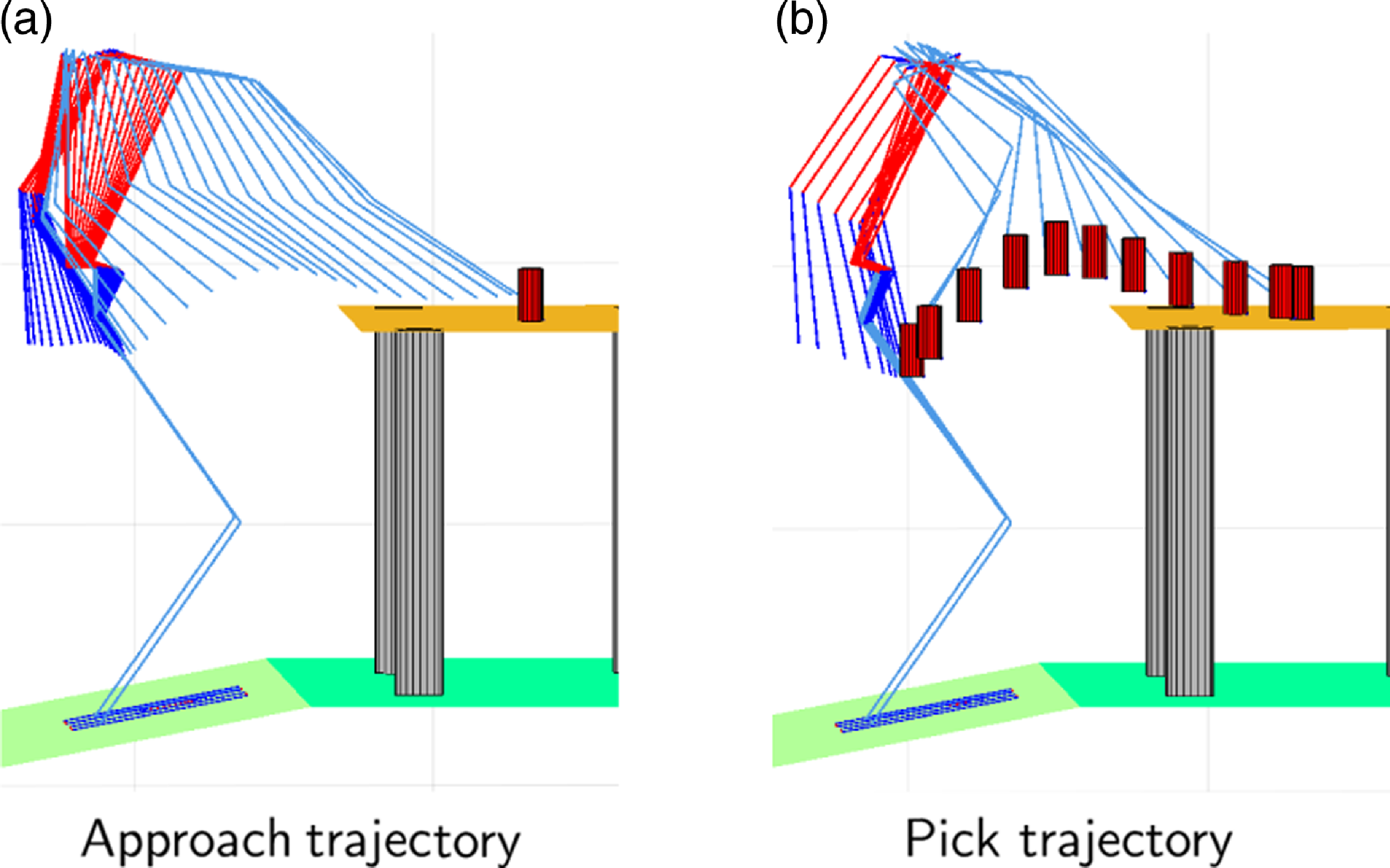
was run for several iterations and results in same pattern in the trajectories. Figure 5a and 5b shows the trajectories for approach and pick, respectively. The same is repeated for Figure 6. Undesirable motion patterns which is a case of elbow up position are seen in Figures 5b and 6b. These undesirable patterns are avoided by setting the weights
 $k_6$
,
 $k_7$
, and
 $k_8$
equal. So
 $\boldsymbol {k}_{opt}$
is modified as
 $\boldsymbol {k}_{opt} = \begin{bmatrix} 1 & 1 & k_3 & k_4 & k_5 & k_6 & k_6 & k_6 \end{bmatrix}$
. So,
 $k_{opt}$
contains only four independent variables number of optimization variables,
 $nvars$
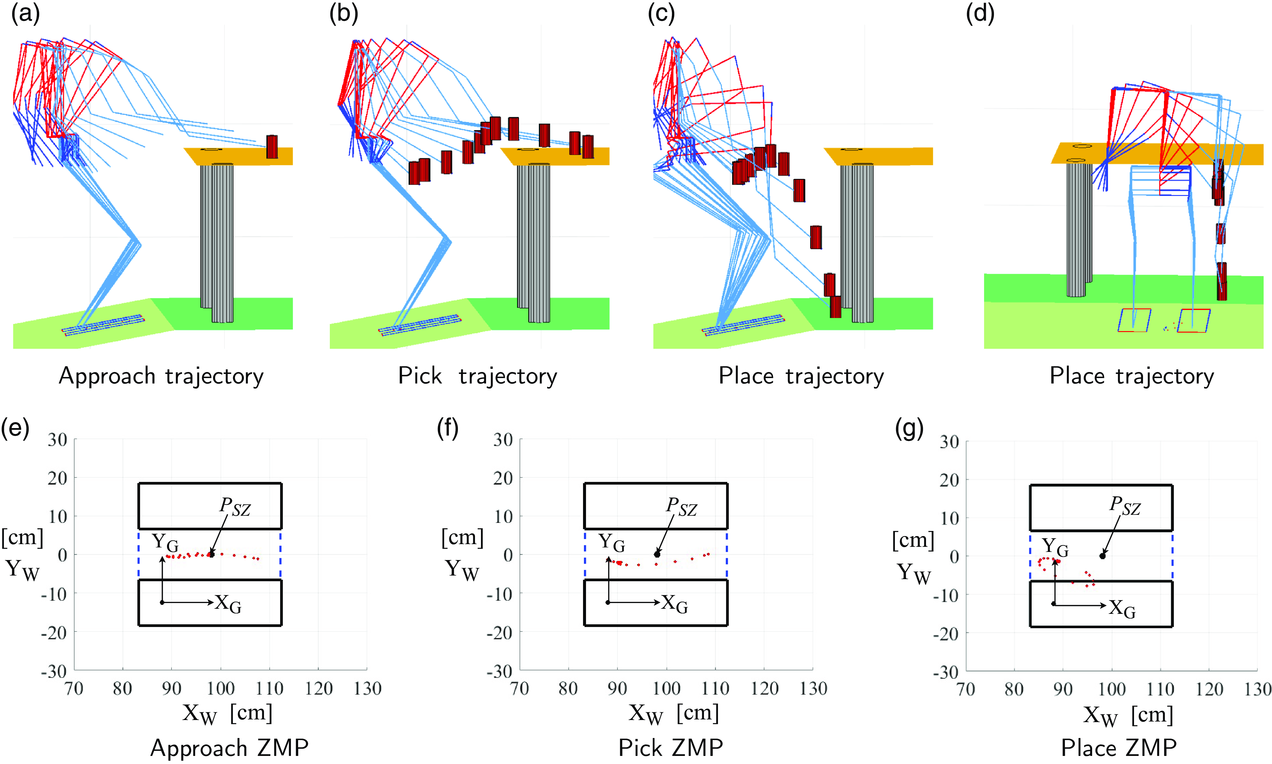
mentioned in Section 4 is 16. Trajectories for approach, pick, and place, and the respective optimization curves are shown in Figure 7a, Figure 7b, and Figure 7c. The objective function Eq. (19) is a function of work done and penalties for violating collision constraints and ZMP constraints. Initially, when the optimization begins, penalty terms dominate over the work done term. Work done term starts dominating when the curve begins to converge and finally only the work done term remains when the curve is fully converged. Figure 7d, 7e, and 7f shows optimization curves during approach, pick, and place, respectively, with respective work done as 51.67 joules, 17.15 joules, and 110.9 joules. In Eq. (21), the value of
 $\gamma _1 = 0$
when the ZMP is inside the support polygon otherwise
 $\gamma _1 = 10$
.
Different optimization curve during place (stage III) for
 $\boldsymbol {k}_{opt} = \begin{bmatrix} 1 & 1 & k_3 & k_4 & k_5 & k_6& k_6 & k_6 \end{bmatrix}$
.

Two task (
 $\mathcal {T}_1$
and
 $\mathcal {T}_3$
) decomposition trajectory and ZMP.

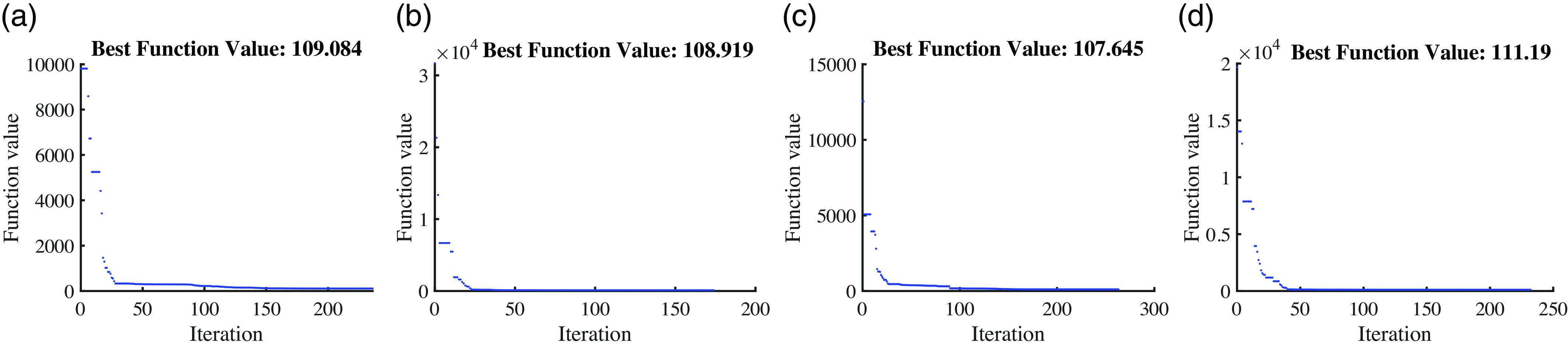
The optimization algorithm for placing the object on the floor for the same object’s location was run several times and approximately results in the same values as shown in Figure 8.
5.2. Case I: three task decomposition
$\mathcal {T}_1, \mathcal {T}_2, \mathcal {T}_3$

The trajectories for the three different stages (approach, pick, and place) of the task are shown in Figure 7a, 7b, and 7c, respectively. In all three stages, the robot was able to perform the primary task of reaching the target without hitting the obstacles. The secondary task, i.e., the desired hip motion is primarily responsible for the dynamic balance of the robot while doing the task. The effect of such is reflected in the ZMP distribution around the point
 $P_{SZ}$
. The plot of respective ZMP inside the support polygon projected on
 $X_WY_W$
-plane is shown in Figure 7g, 7h, and 7i. In all three stages of the task, the ZMP remains well inside the support polygon. The point
 $P_{SZ}$
is located inside the support polygon at (10, 12.5, 0) cm from the origin of frame
 $\{G\}$
. The tertiary task, i.e., maximizing the manipulability of the primary chain while the robot tries to fulfill the primary task and the secondary task is shown in Figure 7j, 7k and 7l. The total work done for all three stages is 179.7 joules. As the task of maximizing the manipulability is of the least priority, manipulability is maximized only in the approach stage and place stage. The surface on which the robot stands has an inclination of
 $-12.3^\circ$
with respect to
 $X_WY_W$
-plane along
 $\hat {\boldsymbol {Y}}_W$
axis. The robot is located at
 ${}^{W}\!\boldsymbol {P}_G = \begin{bmatrix}88 && -12.5 && 20 \end{bmatrix}^T$
cm and
 ${}^{G}\!\boldsymbol {P}_F = \begin{bmatrix}0 && 25 && 0 \end{bmatrix}^T$
cm and at an orientation
 ${}^{W}\!\boldsymbol {\Theta }_G = \begin{bmatrix}0 && \theta _y && 0 \end{bmatrix}^T$
where
 $\theta _y = -12.3^{\circ }$
and
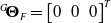 ${}^{G}\!\boldsymbol {\Theta }_F = \begin{bmatrix}0 && 0 && 0 \end{bmatrix}^T$
. The object is located at
 $(160,-50,97)$
cm and destination is at
 $(130,-22,31)$
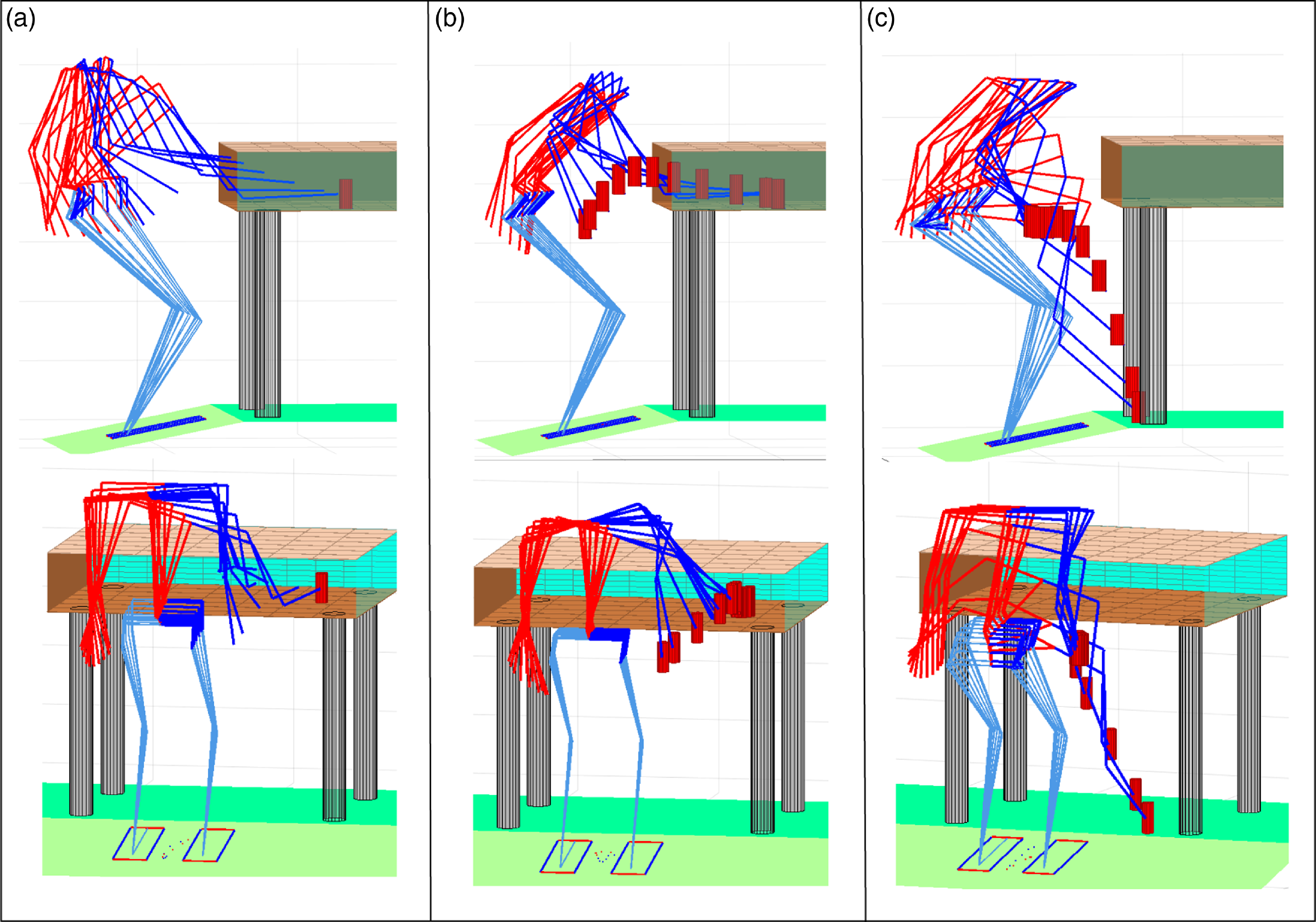
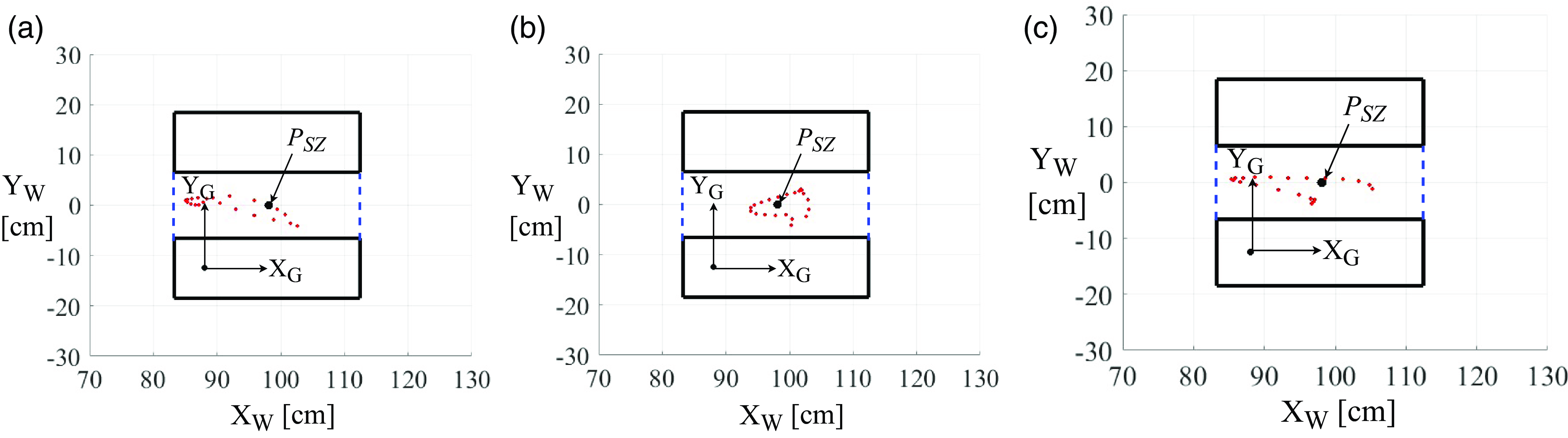
cm. The work is further extended for picking up the object from a cupboard shelf with a 20 cm gap for different object’s locations and destination’s locations as shown in Figure 11 with ZMP plot in Figure 12. Trajectory and ZMP plot for the slope of the inclined plane of
 $\theta _y = 5^{\circ }$
is shown in Figure 13.
5.3. Case II: two task decomposition
$\mathcal {T}_1$
and
$\mathcal {T}_3$


To execute only subtasks
 $\mathcal {T}_1$
and
 $\mathcal {T}_3$
, the Eq. (3) is modified as Eq. (24) and
 $\boldsymbol {k}_{opt}$
is written as
 $\boldsymbol {k}_{opt} = \begin{bmatrix} k _1 & k_2 & k_3 & k_4 & k_5 & k_6 & k_6 & k_6\end{bmatrix}^T$
containing six independent variables. So, the number of optimization variables
 $nvars$
is 12.
 \begin{equation} \boldsymbol {\dot {q}}_d = \boldsymbol {J}_1^{\dagger }\dot {\boldsymbol {r}}_1 + (\boldsymbol {I}_8-\boldsymbol {J}_1^{\dagger }\boldsymbol {J}_1)\boldsymbol {k} \end{equation}
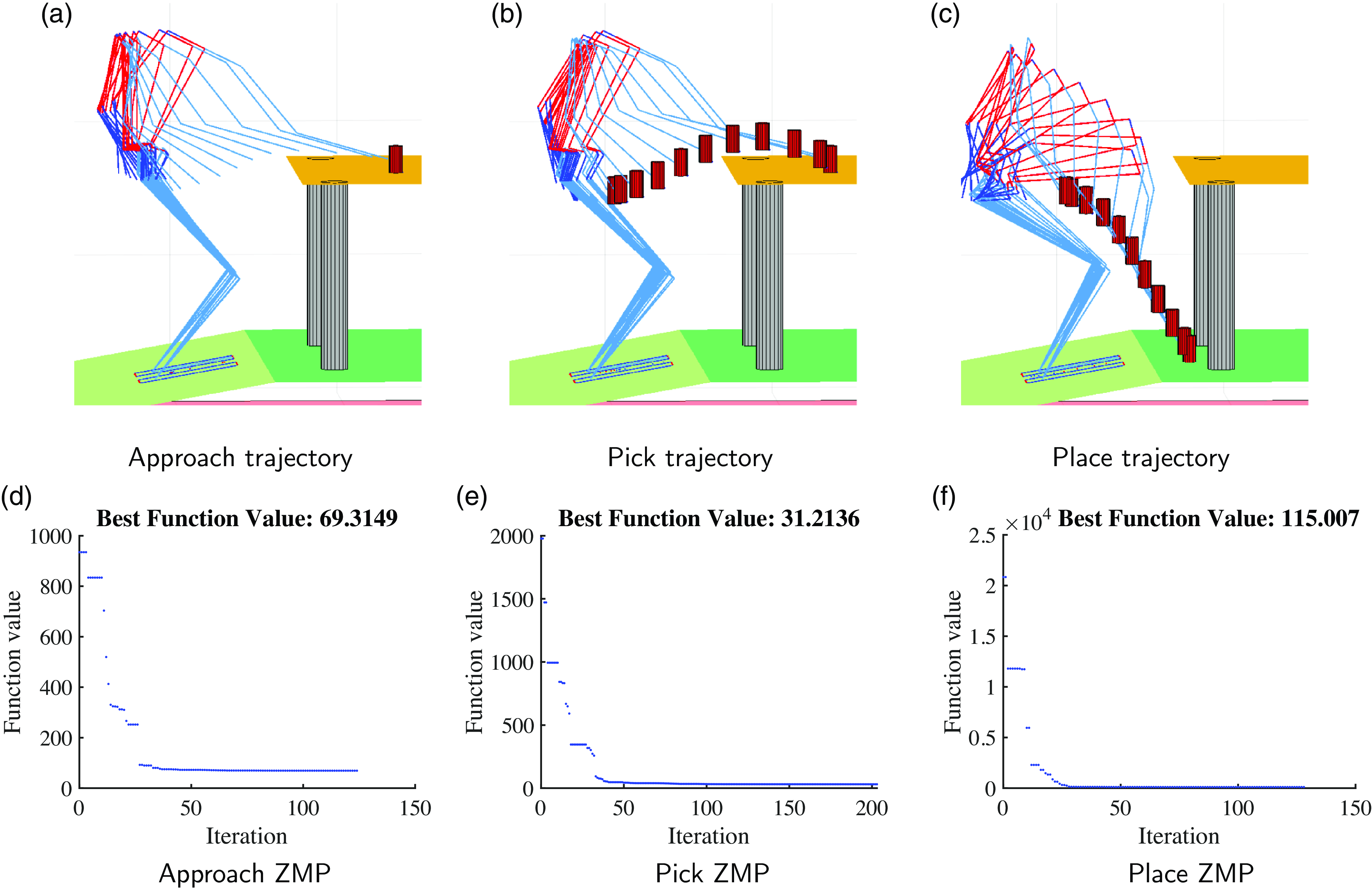
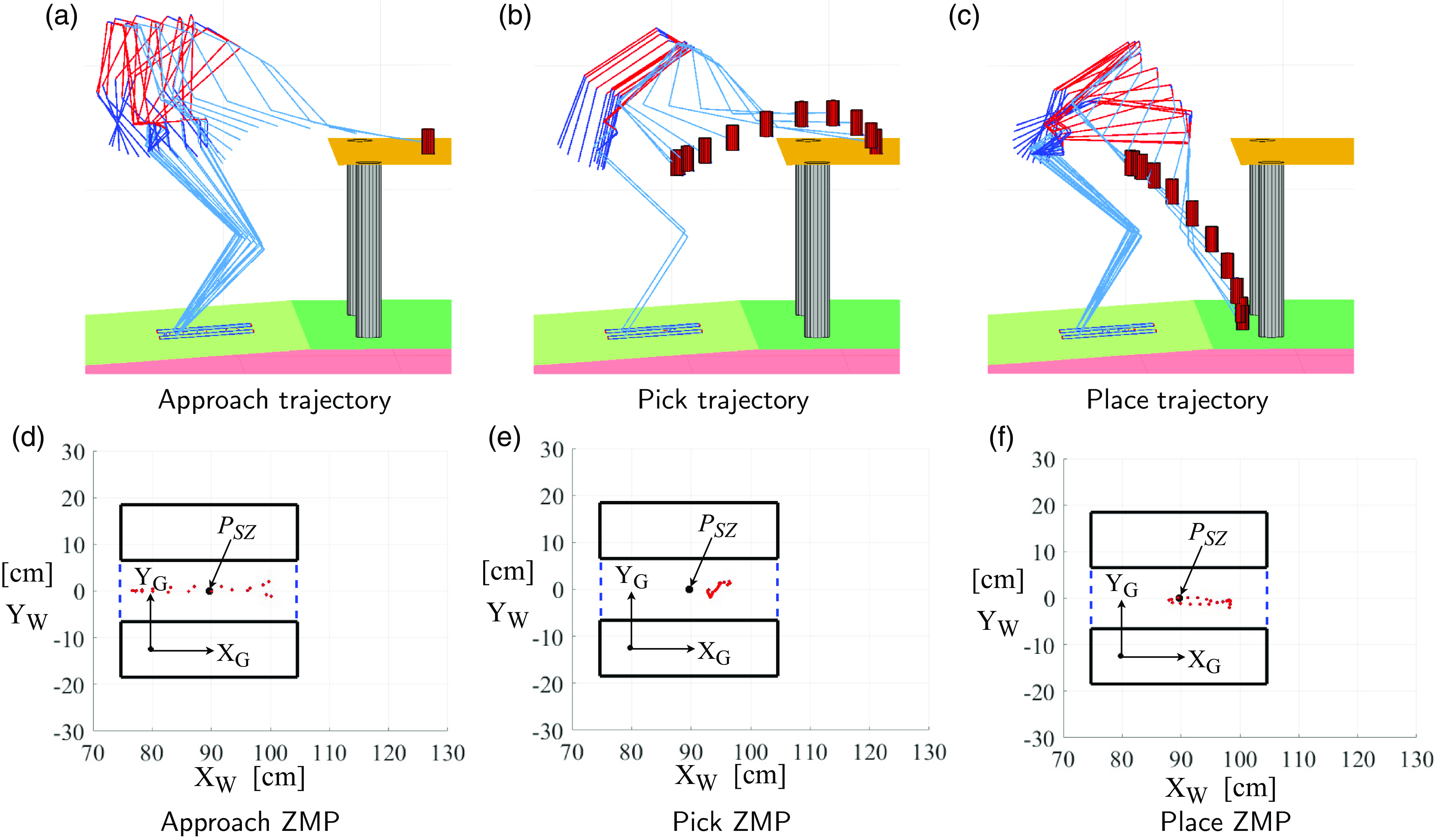
Figure 9 is the case of subtask
 $\mathcal {T}_1$
and subtask
 $\mathcal {T}_3$
. Total energy consumed is 215 joules, which is higher than that of Case I Section 5.2.
Two task (
 $\mathcal {T}_1$
and
 $\mathcal {T}_2$
) decomposition trajectory and ZMP.

5.4. Case III: two task decomposition
$\mathcal {T}_1$
and
$\mathcal {T}_2$


The third term in Eq. (3) vanishes for subtasks
 $\mathcal {T}_1$
and
 $\mathcal {T}_2$
, and number of optimization variables
 $nvars$
is 12. The robot was able to reach the object without losing balance; however, it was not able to place the object on the floor without self-collision as there are not enough variables to impose constraints on the body configurations Figure 10. An undesirable motion pattern is seen in Figure 10d.
Trajectories for the three different stages of the task from a shelf of 20 cm gap. (a) Stage I: Approaching the object located at (155, −40, 97) cm. (b) Stage II: Picking up the object from the shelf located at (155, −40, 97) cm. (c) Stage III: Placing the object on the floor at (125, −35, 27) cm.

ZMP plot for pick and place from a shelf. (a) Approaching the object located at (155, −40, 97) cm. (b) Picking up the object from the shelf located at (155, −40, 97) cm. (c) Placing the object on the floor at (125, −35, 27) cm.

Trajectory and ZMP plot for slope of inclined surface
 $\theta _y = 5^{\circ }$
.

6. Conclusion
In this study, a combination of the Pseudoinverse method of the Jacobian matrix for redundancy resolution and PSO is used to determine an energy-efficient, dynamically balanced trajectory without any collisions with the environment for the pick and place of an object by a humanoid robot standing on inclined ground. Balance is maintained on the inclined ground using ZMP criteria. The key contribution lies in the minimum number of task decomposition and the integration of the entire body dynamics of the humanoid robot (a tree-type robot) to solve the pick and place problem. The robot’s entire task is broken down into three distinct subtasks which are optimized using PSO. Comparisons were made with two task decomposition, and results show that the robot consumed more energy or had undesirable motion when only two tasks were considered. We can conclude that in the case of humanoid robots, a minimum of three task decomposition is required for pick and place application. Increasing the number of task decomposition will still be able to solve the problem. The fourth task could be joint limits on the body of the robot, which is not discussed in our work. In our case, to reduce complexity, the joint limit on the body is set as a constraint in the optimization algorithm. The result shows that the robot can pick and place an object using an energy-optimal trajectory from a table and an enclosed space.
Author contributions
Both the authors James Sorokhaibam and Dr. Ashish Dutta contributed to this research. James Sorokhaibam contributed to the design of the complete algorithm (method), the dynamics of the tree-type robot, implementation, and the simulation. Dr. Ashish Dutta contributed to the trajectory planning, task decomposition, and reviewing and editing the whole paper.
Financial support
This research received no specific grant from any funding agency, commercial, or not-for-profit sectors.
Competing interests
The authors declare no conflicts of interest exist.
Ethical approval
Not applicable under the heading.