





1. Introduction
Work of Hahn, Raksit and Wilson [Reference Hahn, Raksit and WilsonHRW22] extends the notions of prismatic cohomology and syntomic cohomology to the setting of
 $\mathbb{E}_\infty$
-rings. This produces a new tool for computing topological cyclic homology and, consequently, algebraic K-theory. In the present paper, we use this tool to compute the A(1)-homotopy (cf. Notation 2.20) of the algebraic K-theory of the
 $\mathbb{E}_\infty$
-ring ko, known as connective real K-theory. Throughout, we work at the prime
 $p=2$
.
This paper continues the program from [Reference Ausoni and RognesAR02], examining the arithmetic of ring spectra through the lens of telescopically localized algebraic K-theory. In particular, the second and third authors have put forward, in a bundle of predictions known as the redshift conjectures [Reference Ausoni and RognesAR08], the assertion that algebraic K-theory increases chromatic complexity by one. This has now been proven in a qualitative form, for all
 $\mathbb{E}_\infty$
-rings, in a tour de force by Burklund, Schlank and Yuan [Reference Burklund, Schlank and YuanBSY22], building on [Reference YuanYua26, Reference Clausen, Mathew, Naumann and NoelCMN+24] and [Reference Land, Mathew, Meier and TammeLMM+24].
To better understand the arithmetic of
 $\mathbb{E}_\infty$
-rings, it is still desirable to prove more quantitative forms of the redshift conjectures, such as the one originally appearing as the ‘chromatic redshift problem’ in [Reference RognesRog00]. In the present paper, we solve this problem in the case of ko. Explicitly, we prove the following theorem.
Theorem A (Theorem 7.2). The A(1)-homotopy
 $A(1)_* \operatorname{TC}(\mathrm{ko})$
of the topological cyclic homology of ko is a
 $\mathbb{Z}/4[v_2^{32}]$
-module. The associated graded
 \begin{align*}\operatorname{Gr}_{\mathrm{mot}}^* A(1)_* \operatorname{TC}(\mathrm{ko}) &\cong \mathbb{F}_2\{ v_2^i \mid 0 \leqslant i \equiv 0, 1 \ \mathrm{mod}\ 4 \} \\ &\quad\oplus \mathbb{F}_2[v_2] \{\partial, \varsigma, \nu, \lambda'_1, w, \lambda_2 \} \\ &\quad\oplus \mathbb{F}_2[v_2] \{ \varsigma \nu, \nu^2, \partial \lambda_2, \nu w, \nu \lambda_2, \lambda'_1 \lambda_2 \} \\ &\quad\oplus \mathbb{F}_2\{ v_2^j \nu^2 w \mid 0 \leqslant j \equiv 2, 3 \ \mathrm{mod}\ 4 \}\end{align*}
of its descending motivic filtration
 $\operatorname{Fil}_{\mathrm{mot}}^{\star} A(1)_* \operatorname{TC}(\mathrm{ko})$
is a finitely generated and free
 $\mathbb{F}_2[v_2^4]$
-module of rank 52. Here,
 $|\partial| = -1$
,
 $|\varsigma| = 1$
,
 $|\nu| = 3$
,
 $|\lambda'_1|= |w| = 5$
,
 $|v_2| = 6$
and
 $|\lambda_2| = 7$
.
This calculation is carried out by first computing the syntomic cohomology with A(1)-coefficients, alias modulo
 $(2, \eta,v_1)$
, of connective real K-theory.
Theorem B (Theorem 6.12). The syntomic cohomology modulo
 $(2, \eta, v_1)$
of ko is
 \begin{align*}\overline{A}(1)_* \operatorname{gr}_{\mathrm{mot}}^* \operatorname{TC}(\mathrm{ko}) :=&\, \pi_* ( \overline{A}(1) \otimes \operatorname{gr}_{\mathrm{mot}}^* \operatorname{TC}(\mathrm{ko}) ) \\\cong&\, \mathbb{F}_2[v_2] \{1, \partial, \varsigma, \nu, \lambda'_1, w, \lambda_2, \varsigma \nu, \nu^2, \partial \lambda_2, \nu w, \nu \lambda_2, \lambda'_1 \lambda_2, \nu^2 w \} ,\end{align*}
where the (stem, motivic filtration) bidegrees of the
 $\mathbb{F}_2[v_2]$
-module generators are as displayed in Figure 1 and Table 1.
The
 $\mathbb{F}_2[v_2]$
-basis for the syntomic cohomology modulo
 $(2, \eta, v_1)$
of ko, with lines of slope
 $-1$
, 1 and
 $1/3$
indicating multiplication by
 $\partial$
,
 $\eta$
and
 $\nu$
, respectively.

Bidegrees and detecting classes for the
 $\mathbb{F}_2[v_2]$
-module generators of
 $\overline{A}(1)_*\operatorname{gr}_{\mathrm{mot}}^*\operatorname{TC}(\mathrm{ko})$
.

See Notation 7.1 for the algebraic filtration
 $\operatorname{Fil}_{\mathrm{mot}}^{\star} (-)$
on
 $A(1)_* \operatorname{TC}(\mathrm{ko})$
and its associated graded
 $\operatorname{Gr}_{\mathrm{mot}}^* (-)$
, see Definition 2.18 for the spectrum level filtration
 $\operatorname{fil}_{\mathrm{mot}}^{\star} (-)$
on
 $\operatorname{TC}(\mathrm{ko})$
and its associated graded
 $\operatorname{gr}_{\mathrm{mot}}^* (-)$
, and see Construction 2.29 for the meaning of
 $\overline{A}(1) \otimes (-):= \operatorname{gr}_{\mathrm{ev}/\mathbb{S}}^* A(1) \otimes_{\operatorname{gr}_{\mathrm{ev}}^* \mathbb{S}} (-)$
.
As a consequence, we determine the A(1)-homotopy of the algebraic K-theory of ko and of its 2-completion
 $\mathrm{ko}^\wedge_2$
.
Theorem C (Theorems 7.4 and 7.5). There are exact sequences of
 $\mathbb{Z}/4[v_2^{32}]$
-modules
 \begin{align*}0 \to \Sigma^3 \mathbb{F}_2 \longrightarrow A(1)_* \operatorname{K}(\mathrm{ko}) &\overset{\mathrm{trc}}\longrightarrow A(1)_* \operatorname{TC}(\mathrm{ko}) \longrightarrow \mathbb{F}_2\{\partial, \varsigma\} \to 0\end{align*}
and
 \begin{align*}0 \to \Sigma^1 \mathbb{F}_2 \oplus \Sigma^3 \mathbb{F}_2 \longrightarrow A(1)_* \operatorname{K}(\mathrm{ko}^\wedge_2) &\overset{\mathrm{trc}}\longrightarrow A(1)_* \operatorname{TC}(\mathrm{ko}) \longrightarrow \mathbb{F}_2\{\partial, \varsigma\} \to 0 ,\end{align*}
with
 $|\partial| = -1$
and
 $|\varsigma| = 1$
.
Using this, we show in Corollary 7.6 that there is no
 $\mathbb{E}_0$
-ring map
 $\operatorname{K}(\mathrm{ko}) \to\mathrm{tmf}$
, i.e., no spectrum map inducing an isomorphism on
 $\pi_0$
. In contrast, an
 $\mathbb{E}_\infty$
-ring map
 $\operatorname{K}(\mathrm{ko})\to E_2$
is guaranteed to exist by [Reference Burklund, Schlank and YuanBSY22]. Here, tmf denotes the topological modular forms spectrum, and
 $E_2$
is a suitable height 2 Lubin–Tate theory.
As usual, we let K(n) denote the (2-primary) height n Morava K-theory, with coefficient ring
 $K(n)_* = \mathbb{F}_2[v_n^{\pm 1}]$
, and we let
 $L_n$
and
 $L_n^f$
denote Bousfield localization at
 $K(0) \oplus\cdots \oplus K(n)$
and at
 $T(0) \oplus \cdots \oplus T(n)$
, respectively, where
 $T(m) = v_m^{-1} F(m)$
is the telescope of any
 $v_m$
self-map of a type m finite 2-local spectrum F(m).
We say that a spectrum X satisfies the (strong, 2-primary) height n telescope conjecture if the canonical map
 $L_n^fX \to L_n X$
is an equivalence. By recent groundbreaking work of Burklund, Hahn, Levy and Schlank [Reference Burklund, Hahn, Levy and SchlankBHL+23], we know for each
 $n\geqslant2$
that not all spectra have this property. However, it is still interesting to consider the question of which spectra do satisfy this conjecture (see, e.g., [Reference Mahowald and RezkMR99, Conjecture 7.3]). In Theorem 7.7, we deduce from [Reference Hahn, Raksit and WilsonHRW22] and [Reference Clausen, Mathew, Naumann and NoelCMN+20] that the spectra
 $\operatorname{K}(\mathrm{ko})$
,
 $\operatorname{K}(\mathrm{ko}^\wedge_2)$
and
 $\operatorname{TC}(\mathrm{ko})$
all satisfy the height 2 telescope conjecture.
We say that a spectrum X has telescopic complexity n if the map
 $X \to L_n^f X$
is an equivalence in all sufficiently large degrees. In [Reference Ausoni and RognesAR08], the redshift conjecture was phrased in terms of this property. In Theorem 7.8, we apply our Theorems A and C to confirm that the spectra
 $\operatorname{K}(\mathrm{ko})_{(2)}$
,
 $\operatorname{K}(\mathrm{ko}^\wedge_2)_{(2)}$
and
 $\operatorname{TC}(\mathrm{ko})_{(2)}$
(as well as their 2-completions) have telescopic complexity 2, as predicted.
1.1 Organization
In § 2, we give a presentation for the associated graded
 $\operatorname{gr}_{\mathrm{mot}}^* \operatorname{THH}(\mathrm{ko})$
of the motivic filtration on
 $\operatorname{THH}(\mathrm{ko})$
, and calculate its bigraded homotopy modulo
 $(2, \eta, v_1)$
and modulo
 $(2, v_1)$
. In § 3, we compare two filtrations leading to spectral sequences calculating the associated graded objects
 $\operatorname{gr}_\mathrm{mot}^*\operatorname{TC}^{-}(\mathrm{ko})$
and
 $\operatorname{gr}_\mathrm{mot}^* \operatorname{TP}(\mathrm{ko})$
of the motivic filtrations on
 $\operatorname{TC}^{-}(\mathrm{ko})$
and
 $\operatorname{TP}(\mathrm{ko})$
, with appropriate finite coefficients. In § 4, we show how some homotopy classes from A(1) are detected in homotopy modulo
 $(2, \eta,v_1)$
of
 $\operatorname{gr}_{\mathrm{mot}}^* \operatorname{TC}^{-}(\mathrm{ko})$
. In § 5, we study the
 $\mathbb{T}$
-Tate spectral sequence calculating prismatic cohomology, i.e., the homotopy modulo
 $(2, v_1, v_2)$
and
 $(2, \eta, v_1, v_2)$
of
 $\operatorname{gr}_{\mathrm{mot}}^* \operatorname{TP}(\mathrm{ko})$
. In § 6, we study the
 $\mathbb{T}$
-homotopy fixed point spectral sequence calculating the homotopy of
 $\operatorname{gr}_{\mathrm{mot}}^* \operatorname{TC}^{-}(\mathrm{ko})$
modulo
 $(2, v_1, v_2)$
and
 $(2, \eta,v_1, v_2)$
, and use this to calculate syntomic cohomology, i.e., the homotopy of
 $\operatorname{gr}_{\mathrm{mot}}^* \operatorname{TC}(\mathrm{ko})$
modulo
 $(2, v_1)$
and
 $(2, \eta,v_1)$
. Finally, in § 7, we determine the differential pattern in the motivic spectral sequence calculating
 $A(1)_* \operatorname{TC}(\mathrm{ko})$
, and use known facts about the cyclotomic trace map to deduce corresponding results for
 $A(1)_* \operatorname{K}(\mathrm{ko}^\wedge_2)$
and
 $A(1)_* \operatorname{K}(\mathrm{ko})$
.
1.2 Conventions
We let
 $\mathcal{A}$
and
 $\mathcal{A}^\vee$
denote the mod 2 Steenrod algebra and its dual, respectively. We set
 $H_* (X) := H_* (X; \mathbb{F}_2)$
and write
 \begin{align*}\nu \colon H_* (X) \longrightarrow \mathcal{A}^\vee \otimes H_* (X) \end{align*}
for the
 $\mathcal{A}^\vee$
-coaction. We write
 $\mathcal{A}(1)$
for the subalgebra of
 $\mathcal{A}$
generated by
 $Sq^1$
and
 $Sq^2$
, and note that
 $\mathcal{A}(1)^\vee= \mathbb{F}_2[\xi_1, \xi_2]/(\xi_1^4, \xi_2^2)$
.
We say that a spectrum X is even if its homotopy groups
 $\pi_*(X)= X_*$
are concentrated in even degrees.
Let
 $\mathbb{Z}^{\mathrm{op}}$
be the category whose objects are integers, such that
 $\operatorname{Mor}_{\mathbb{Z}^{\mathrm{op}}}(n,m) = *$
if
 $n\geqslant m$
and
 $= \varnothing$
otherwise. Let
 $\mathbb{Z}^{\delta}$
be the integers as a discrete category. Given a presentably symmetric monoidal stable
 $\infty$
-category
 $\mathcal{C}$
, we write
 \begin{align*}\mathcal{C}^{\operatorname{fil}} :=\operatorname{Fun}(\mathbb{Z}^{\mathrm{op}}, \mathcal{C}),\quad \mathcal{C}^{\operatorname{gr}} := \operatorname{Fun}(\mathbb{Z}^{\delta}, \mathcal{C}) . \end{align*}
Given
 $I^{\star} \in \mathcal{C}^{\operatorname{fil}}$
and
 $J^* \in \mathcal{C}^{\operatorname{gr}}$
, we write
 $I^w := I(w)$
and
 $J^w := J(w)$
. We recall that there is a symmetric monoidal functor
 \begin{align*} \operatorname{gr}^*\colon \mathcal{C}^{\operatorname{fil}} \longrightarrow \mathcal{C}^{\operatorname{gr}} \end{align*}
defined on an object
 $I^{\star}$
by
 $\operatorname{gr}^w I = I^w /I^{w+1}$
. As in the above notation, for consistency we use the superscript
 $\star$
as in
 $I^{\star}$
for a filtered object, the superscript
 $*$
as in
 $J^*$
for a graded object, and a superscript
 $\bullet$
as in
 $K^{\bullet}$
for a cosimplicial object. In § 3, we also use increasing filtrations and homological grading, in which case
 $\operatorname{fil}_w := \operatorname{fil}^{-w}$
and
 $\operatorname{gr}_w := \operatorname{gr}^{-w}$
.
We use the terminology from [Reference IsaksenIsa19, Definition 4.1.2] for (hidden) extensions in spectral sequences. We use the term ‘algebra spectral sequence’ in the sense of [Reference Hedenlund and RognesHR24, Definition 4.9], and we will also consider module spectral sequences over such algebra spectral sequences.
In §§ 2–6, we use the following conventions. We write
 $\operatorname{THH}(A/R) = |[q] \mapsto A \otimes_R \cdots \otimes_R A|$
for the relative topological Hochschild homology of an R-algebra A, with
 $q+1$
copies of A in simplicial degree q, and we simply write
 $\operatorname{THH}(A)$
when
 $R = \mathbb{S}$
. We implicitly 2-complete each of the following invariants:
 $\operatorname{THH} := \operatorname{THH}(-)^\wedge_2$
,
 $\operatorname{TC}^{-} := ( \operatorname{THH}(-)^{h\mathbb{T}})^\wedge_2$
,
 $\operatorname{TP} := ( \operatorname{THH}(-)^{t\mathbb{T}} )^\wedge_2$
,
 $\operatorname{TC} := \operatorname{TC}(-)^\wedge_2$
and
 $\operatorname{K} := \operatorname{K}(-)^\wedge_2$
. We write ko, ku, KU, MU, MUP,
 $\mathbb{S}$
and BP for the 2-completions of connective real K-theory, connective complex K-theory, periodic complex K-theory, complex cobordism, periodic complex cobordism, the sphere spectrum and the Brown–Peterson spectrum, respectively. We will simply write
 $\mathbb{Z}$
for the 2-adic integers. We write
 $\mathrm{Sp}_2$
for the
 $\infty$
-category of 2-complete spectra with symmetric monoidal product
 $\otimes$
. Note that our smash product is implicitly 2-completed in §§ 2–6, so that
 $\otimes_R :=(- \otimes_R - )^\wedge_2$
for any 2-complete
 $\mathbb{E}_\infty$
-ring R, and we omit R from the notation when R is the 2-complete sphere spectrum. We also write
 $\otimes$
for the (underived) tensor product over the 2-adic integers and expect the intended meaning to be clear from the context. We write
 $\mathbb{T}$
for the circle regarded as the group of complex numbers of modulus 1, and we set
 $\mathcal{C}^{B\mathbb{T}} := \operatorname{Fun}(B\mathbb{T}, \mathcal{C})$
. We write
 $C_2 = \{\pm 1\}\subset \mathbb{T}$
for the subgroup of order 2.
In § 7, as in the present § 1, we explicitly include notation for 2-completion, especially in the argument of
 $\operatorname{K}(-)$
. Note that the canonical map
 $\operatorname{TC}(\mathrm{ko})^\wedge_2\to \operatorname{TC}(\mathrm{ko}^\wedge_2)^\wedge_2$
is an equivalence by [Reference MadsenMad94, pp. 274–275] (cf. [Reference Nikolaus and ScholzeNS18, pp. 351–352]), so we can omit 2-completion in the argument of
 $\operatorname{TC}(-)^\wedge_2$
.
2. Hochschild homology and motivic filtrations
We first introduce filtrations on
 $\operatorname{THH}$
,
 $\operatorname{TC}^{-}$
,
 $\operatorname{TP}$
and
 $\operatorname{TC}$
. The reader is encouraged to read [Reference Bökstedt, Hsiang and MadsenBHM93, Reference Bökstedt and MadsenBM94, Reference Bökstedt and MadsenBM95, Reference Hesselholt and NikolausHN20] for background on these invariants and [Reference Hahn, Raksit and WilsonHRW22] for a thorough account of the filtrations that we use in this paper.
Definition 2.1. Given a map
 $f \colon A \to B$
of 2-complete
 $\mathbb{E}_\infty$
-rings, we write
 $C^{\bullet}(B/A)$
for the associated cosimplicial Amitsur complex with
 $C^q(B/A) = B^{\otimes_A q+1}$
.
Recall that there is a map of
 $\mathbb{E}_\infty$
-rings
 $c \colon \mathrm{ko} \to \mathrm{ku}$
called the complexification map, where
 $\mathrm{ko}_* = \mathbb{Z}[\eta, A, B]/(2\eta,\eta^3, \eta A, A^2-4B)$
,
 $\mathrm{ku}_* = \mathbb{Z}[u]$
,
 $A \mapsto 2 u^2$
and
 $B\mapsto u^4$
, with
 $|\eta| = 1$
,
 $|A| = 4$
,
 $|B| = 8$
and
 $|u| =2$
.
Lemma 2.2.
There exists an
 $\mathbb{E}_\infty$
-ring map
 $\mathrm{MU} \to \mathrm{ku}$
. We can choose the generators of
 $\mathrm{MU}_* = \pi_*(\mathrm{MU}) = \mathbb{Z}[x_i \mid i\geqslant1]$
so that
 $x_1 \mapsto u$
and
 $x_i \mapsto 0$
for each
 $i\geqslant2$
. Here,
 $|x_i| = 2i$
.
Proof. The proof of [Reference Hahn and YuanHY20, Theorem 4.3] shows the existence of
 $\mathbb{E}_\infty$
-ring maps
 $\mathrm{MU} \to \mathrm{MUP} \to \mathrm{KU}$
. Passing to connective covers gives the factorization through ku. Recall our running convention that
 $\mathbb{Z}$
denotes the 2-adic integers. Both MU and ku have first Postnikov k-invariant the generator of
 $H^3(H\mathbb{Z}; \mathbb{Z}) \cong \mathbb{Z}/2$
, so
 $\mathbb{Z}\{x_1\} = \pi_2(\mathrm{MU}) \to \pi_2(\mathrm{ku}) = \mathbb{Z}\{u\}$
must be an isomorphism. Dividing the first choice of
 $x_1$
by a unit, we can assume that
 $x_1 \mapsto u$
. For each
 $i\geqslant2$
, we can then subtract a multiple of
 $x_1^i$
from the first choice of
 $x_i$
to ensure that
 $x_i \mapsto 0$
.
We hereafter fix
 $\mathrm{MU} \to \mathrm{ku}$
and the
 $x_i$
as in the above lemma. This provides
 $\mathbb{E}_\infty$
-ring maps
 $C^q(\mathrm{MU}/\mathbb{S}) \to C^q(\mathrm{ku}/\mathrm{ko})$
, compatibly for all
 $q \geqslant 0$
. We write
 \begin{align*}\tau_{\geqslant \star} \colon \mathrm{Sp}_2\longrightarrow \mathrm{Sp}_2^{\operatorname{fil}} \end{align*}
for the monoidal Whitehead filtration [Reference LurieLur17, Proposition 1.4.3.6, Example 2.2.1.10]. Note that the circle group
 $\mathbb{T}$
acts freely on
 $S^1 \subset S^{3} \subset \cdots \subset S^{\infty} = E\mathbb{T}$
. We write
 $F(S^{2\ell+1}_+, \operatorname{THH})^{\mathbb{T}}$
for the
 $\ell$
th-order approximate fixed points functor, taking
 $A/R$
to
 $F(S^{2\ell+1}_+,\operatorname{THH}(A/R))^{\mathbb{T}} \simeq \lim_{\mathbb{C}\mathrm{P}^\ell} \operatorname{THH}(A/R)$
, as in [Reference Bruner and RognesBR05, § 2] and [Reference Angelini-Knoll, Ausoni, Culver, Höning and RognesAAC+25, § 7]. Here,
 $\mathbb{C}\mathrm{P}^\ell \subset \mathbb{C}\mathrm{P}^\infty = B\mathbb{T}$
. We also write
 $\operatorname{THH}^{hC_2}$
and
 $\operatorname{THH}^{tC_2}$
for the functors obtained by applying
 $C_2$
-homotopy fixed points and the
 $C_2$
-Tate construction to
 $\operatorname{THH}$
, respectively.
Definition 2.3. For
 $F \in \{\operatorname{THH}, \operatorname{TC}^{-}, \operatorname{TP}, F(S^{2\ell+1}_+,\operatorname{THH})^{\mathbb{T}},\operatorname{THH}^{hC_2},\operatorname{THH}^{tC_2}\}$
we define
 $\mathbb{E}_\infty$
algebras
 \begin{align*}\operatorname{fil}_{\mathrm{mot}}^{\star} F(\mathrm{ko}) & :=\operatorname{Tot} (\tau_{\geqslant 2\star}F(C^{\bullet}(\mathrm{ku}/\mathrm{ko})/C^{\bullet}(\mathrm{MU}/\mathbb{S}))), \\\operatorname{gr}_{\mathrm{mot}}^* F(\mathrm{ko}) & :=\operatorname{gr}^* (\operatorname{fil}_{\mathrm{mot}}^{\star}F(\mathrm{ko}))\end{align*}
in
 $\mathrm{Sp}_2^{\operatorname{fil}}$
and
 $\mathrm{Sp}_2^{\operatorname{gr}}$
, respectively. Here,
 $\operatorname{Tot}$
denotes the totalization of a cosimplicial object. We refer to
 $\operatorname{gr}_{\mathrm{mot}}^w\operatorname{TP}(\mathrm{ko})$
as the weight w prismatic cohomology spectrum of ko and to
 $\pi_* \operatorname{gr}_{\mathrm{mot}}^w \operatorname{TP}(\mathrm{ko})$
as the weight w prismatic cohomology groups.
Remark 2.4. We will show in Proposition 2.15 that
 \begin{align*} \operatorname{THH}(C^q(\mathrm{ku}/\mathrm{ko}) / C^q(\mathrm{MU}/\mathbb{S}))=C^{q}(\operatorname{THH}(\mathrm{ku}/\mathrm{MU})/\operatorname{THH}(\mathrm{ko})) \end{align*}
is even and 2-torsion free. It follows that
 $F(C^q(\mathrm{ku}/\mathrm{ko}) / C^q(\mathrm{MU}/\mathbb{S}))$
is even for each functor
 $F \in \{\operatorname{THH}, \operatorname{TC}^{-},\operatorname{TP}, F(S^{2\ell+1}_+,\operatorname{THH})^{\mathbb{T}},\operatorname{THH}^{hC_2},\operatorname{THH}^{tC_2}\}$
and
 $q\geqslant 0$
. Hence the double-speed Whitehead filtration in the definition of
 $\operatorname{fil}_{\mathrm{mot}}^{\star} F(\mathrm{ko})$
will be well behaved for each F in the above list.
Remark 2.5. We will verify in Proposition 2.17 that
 $\pi_*\operatorname{gr}_{\mathrm{mot}}^* \operatorname{TP}(\mathrm{ko})$
agrees with prismatic cohomology in the sense of [Reference Hahn, Raksit and WilsonHRW22, Definition 1.3.4], building on [Reference Bhatt, Morrow and ScholzeBMS19].
Remark 2.6. Note that when
 $\operatorname{THH}(A/R)$
is even, we are considering the filtered spectrum defined by
 $\tau_{\geqslant2\star} \operatorname{TP}(A/R) = \tau_{\geqslant 2\star} (\operatorname{THH}(A/R)^{t\mathbb{T}})$
, which is not the same as the filtered spectrum
 $(\tau_{\geqslant 2\star} \operatorname{THH}(A/R))^{t\mathbb{T}}$
. In particular, the class t in the associated graded of the
 $\mathbb{T}$
-Tate filtration, lifting the generator of
 $\pi_{-2} (H\mathbb{F}_2)^{t\mathbb{T}}$
, has weight
 $-1$
(and motivic filtration 0; see below). The same applies for t lifting the generator of
 $\pi_{-2} (H\mathbb{F}_2)^{h\mathbb{T}}$
, in the associated graded of the
 $\mathbb{T}$
-homotopy fixed point filtration for
 $\operatorname{TC}^{-}(A/R)= \operatorname{THH}(A/R)^{h\mathbb{T}}$
.
We also fix terminology for gradings.
Definition 2.7. Given
 $M^* \in \mathrm{Sp}_2^{\operatorname{gr}}$
and
 $x \in \pi_n M^w$
, we say that x has stem n, weight w and motivic filtration
 $2w-n$
, and write
 $\|x\| = (n,2w-n)$
. In [Reference Hahn, Raksit and WilsonHRW22, Definition 1.4.2], stem and motivic filtration are called degree and Adams weight, respectively. We refer to the (Adams indexed, Bousfield–Kan) spectral sequence
 \begin{align*}E_2^{n,2w-n} = \pi_n \operatorname{gr}_{\mathrm{mot}}^w F(\mathrm{ko}) \Longrightarrow \pi_n F(\mathrm{ko}) \end{align*}
for each
 $F \in \{\operatorname{THH}, \operatorname{TC}^{-}, \operatorname{TP},F(S^{2\ell+1}_+,\operatorname{THH})^{\mathbb{T}},\operatorname{THH}^{hC_2}, \operatorname{THH}^{tC_2}\}$
as the motivic spectral sequence. We will show in Lemma 2.19 that the motivic spectral sequence converges in each case.
We plot each motivic spectral sequence with stem on the horizontal axis and motivic filtration on the vertical axis. Given this convention, if
 $\|x\| = (n,2w-n)$
then
 $\|d_r(x)\| = (n-1, 2w-n+r)$
. Note that we write
 $E_r^{n,2w-n}$
where it is also standard to write
 $E_r^{2w-n,2w}$
in the literature. With these conventions, the motivic spectral sequence
 $E_r^{n,s}$
-term is concentrated in internal degrees
 $n+s = 2w$
and, consequently,
 $d_r = 0$
for all even integers
 $r\geqslant 2$
.
Our first aim is to show that the filtrations from Definition 2.3 agree with the motivic filtrations considered in [Reference Hahn, Raksit and WilsonHRW22, Definition 4.2.1].
Definition 2.8 [Reference Hahn, Raksit and WilsonHRW22, Definition 2.2.15(4)]. A map
 $A \to B$
of
 $\mathbb{E}_\infty$
-rings is 2-completely evenly free if for each nonzero even
 $\mathbb{E}_\infty$
A-algebra C of bounded 2-power torsion, the pushout
 $B\otimes_A C$
is equivalent as a C-module to a nonzero wedge sum of even suspensions of C. In what follows, we will omit ‘2-completely’ and simply refer to such maps of
 $\mathbb{E}_{\infty}$
-rings as evenly free maps, to be consistent with our conventions.
Remark 2.9. This condition on
 $B \otimes_A C$
is equivalent to
 $\pi_*(B \otimes_A C)$
being a nonzero free
 $C_*$
-module on generators in even stems. An evenly free map
 $A \to B$
of
 $\mathbb{E}_\infty$
-rings is 2-completely eff (= evenly faithfully flat), in the sense of [Reference Hahn, Raksit and WilsonHRW22, Definition 2.2.15(2)], as per [Reference Hahn, Raksit and WilsonHRW22, Remark 2.2.16].
Lemma 2.10.
The complexification map
 $\mathrm{ko} \to \mathrm{ku}$
is evenly free. Moreover, for each even
 $\mathbb{E}_\infty$
ko-algebra C, there is an isomorphism of
 $C_*$
-algebras
 \begin{align*}\pi_* (\mathrm{ku} \otimes_{\mathrm{ko}} C) \cong C_*[b_1]/(\hat b_1^2) , \end{align*}
where
 $\hat b_1^2 = b_1^2+c_2b_1 +c_4$
for some
 $c_2, c_4 \in C_*$
with
 $|c_2| = 2$
and
 $|c_4| = 4$
.
Proof. Recall the Wood (homotopy) cofiber sequence
 \begin{align} \Sigma \mathrm{ko} \overset{\eta}\longrightarrow \mathrm{ko} \overset{c}\longrightarrow \mathrm{ku} \overset{R}\longrightarrow \Sigma^2\mathrm{ko}\end{align}
of ko-modules, where we write R for the map satisfying
 $R \circ(u\cdot -) = \Sigma^2 r$
, with
 $r \colon \mathrm{ku} \to \mathrm{ko}$
the realification map. The resulting cofiber sequence
 \begin{align*}\Sigma C\overset{\eta}\longrightarrow C \longrightarrow \mathrm{ku} \otimes_{\mathrm{ko}} C \overset{R}\longrightarrow \Sigma^2 C \end{align*}
induces a short exact sequence of
 $C_*$
-modules
 \begin{align} 0 \to C_* \longrightarrow \pi_* (\mathrm{ku} \otimes_{\mathrm{ko}} C) \overset{R}\longrightarrow \Sigma^2 C_* \to 0 ,\end{align}
since C is even, so that
 $\eta \colon \Sigma C_* \to C_*$
is zero. We conclude that
 $ \pi_* (\mathrm{ku} \otimes_{\mathrm{ko}} C)$
is concentrated in even degrees.
A choice of a class
 $b_1 \in \pi_2(\mathrm{ku} \otimes_{\mathrm{ko}} C)$
with
 $R(b_1)= \Sigma^2 1$
is equivalent to a choice of a splitting of (2.2), so that
 $\pi_* (\mathrm{ku} \otimes_{\mathrm{ko}} C) \cong C_* \{1, b_1 \}$
is free over
 $C_*$
and nonzero if
 $C \ne 0$
. Writing
 $\hat b_1^2 = b_1^2+ c_2 b_1 + c_4$
for the monic polynomial that vanishes in
 $\pi_4(\mathrm{ku}\otimes_{\mathrm{ko}} C)$
, there is an isomorphism
 \begin{align*}\pi_* (\mathrm{ku} \otimes_{\mathrm{ko}} C)\cong C_*[b_1]/(\hat b_1^2) \end{align*}
of
 $C_*$
-algebras.
Remark 2.11. Note that
 $c_2$
and
 $c_4$
in the statement of Lemma 2.10 need not be zero. For example, when
 $C= \mathrm{ku}$
, then
 $b_1$
can be chosen as in [Reference Dundas, Lindenstrauss and RichterDLR22, Lemma 5.1] so that
 $\hat b_1^2 = b_1^2-u b_1$
.
Lemma 2.12.
Let
 $A \to B$
be a map of connective
 $\mathbb{E}_\infty$
-rings with bounded 2-power torsion. If
 $\pi_*(B\otimes_A H\pi_0 A)$
is a nonzero, free and even
 $\pi_0 A$
-module, then
 $A \to B$
is evenly free.
Proof. Let C be a nonzero even
 $\mathbb{E}_\infty$
A-algebra of bounded 2-power torsion. Associated to the double-speed Whitehead filtration
 $\tau_{\geqslant2\star} C$
we have an algebra spectral sequence
 $E_1(C) \Longrightarrow \pi_*(C)$
with
 $E_1^{*,w}(C) =\pi_{*-2w}(H \pi_{2w} C)$
. Similarly, the induced filtration
 $B \otimes_A\tau_{\geqslant2\star} C$
yields a spectral sequence
 $E_1(B \otimes_A C)\Longrightarrow \pi_*(B \otimes_A C)$
with
 $E_1^{*,w}(B \otimes_A C) =\pi_{*-2w}(B \otimes_A H\pi_{2w} C)$
, which we view as a module spectral sequence over the first one. Both spectral sequences are conditionally convergent, since A and B are assumed to be connective. A choice of
 $\pi_0 A$
-module basis for
 $\pi_*(B \otimes_A H\pi_0 A)$
, and the equivalence
 \begin{align*}B \otimes_A H\pi_{2w} C \simeq (B \otimes_A H\pi_0 A) \otimes_{H\pi_0 A} H\pi_{2w} C ,\end{align*}
show that
 $E_1(B \otimes_A C) \cong \pi_*(B \otimes_A H\pi_0 A)\otimes_{\pi_0 A} E_1(C)$
is a nonzero free
 $E_1(C)$
-module on generators in (filtration 0 and) even stems. Hence both spectral sequences are concentrated in even stems, collapse at
 $E_1 = E_\infty$
, and are strongly convergent by [Reference BoardmanBoa99, Theorem 8.10]. It follows that the
 $E_1(C)$
-module generators lift to the abutment, giving a
 $\pi_*(C)$
-module basis for
 $\pi_*(B \otimes_A C)$
.
Remark 2.13. Without our implicit 2-completion assumptions and the bounded 2-power torsion assumption, the same argument as in the proof of the above lemma provides a criterion for a map of connective
 $\mathbb{E}_{\infty}$
-rings to be evenly free in the sense of [Reference Hahn, Raksit and WilsonHRW22, Definition 2.2.15(3)].
Proposition 2.14.
The map
 $\operatorname{THH}(\mathrm{ko}) \to \operatorname{THH}(\mathrm{ku}/\mathrm{MU})$
, induced by the complexification map
 $c \colon \mathrm{ko} \to \mathrm{ku}$
and the unit map
 $\mathbb{S} \to \mathrm{MU}$
, is evenly free.
Proof. Since ko, ku and MU are connective and have finite type, it follows that
 $\operatorname{THH}(\mathrm{ko})$
and
 $\operatorname{THH}(\mathrm{ku}/\mathrm{MU})$
have finite type, and therefore have bounded 2-power torsion. Hence, by Lemma 2.12, it suffices to show that
 \begin{align*}\pi_*(\operatorname{THH}(\mathrm{ku}/\mathrm{MU}) \otimes_{\operatorname{THH}(\mathrm{ko})} H\mathbb{Z}) \end{align*}
is a nonzero, free and even
 $\mathbb{Z}$
-module. The
 $\mathbb{E}_\infty$
-ring map
 $\operatorname{THH}(\mathrm{ko}) \to H\mathbb{Z}$
can be rewritten as
 $\operatorname{THH}(\mathrm{ko}/\mathbb{S}) \to\operatorname{THH}(H\mathbb{Z}/H\mathbb{Z})$
, which is induced by
 $\mathrm{ko} \to H\mathbb{Z}$
over
 $\mathbb{S} \to H\mathbb{Z}$
. Then
 \begin{align*}\operatorname{THH}(\mathrm{ku}/\mathrm{MU}) \otimes_{\operatorname{THH}(\mathrm{ko})} H\mathbb{Z} &\cong \operatorname{THH}(\mathrm{ku}/\mathrm{MU}) \otimes_{\operatorname{THH}(\mathrm{ko})} \operatorname{THH}(H\mathbb{Z}/H\mathbb{Z}) \\ &\simeq \operatorname{THH}(\mathrm{ku} \otimes_{\mathrm{ko}} H\mathbb{Z} / \mathrm{MU} \otimes H\mathbb{Z}) ,\end{align*}
where the last equivalence holds because
 $\operatorname{THH}$
commutes with pushouts of
 $\mathbb{E}_\infty$
-rings.
Recall that
 $\pi_*(\mathrm{MU} \otimes H\mathbb{Z}) \cong H_*(\mathrm{MU}; \mathbb{Z}) = \mathbb{Z}[b_k \mid k\geqslant1]$
as
 $\mathbb{Z}$
-algebras, with
 $|b_k| = 2k$
. Since
 $\mathrm{MU} \to \mathrm{ku}$
is 4-connected by Lemma 2.2, and
 $\mathbb{S} \to \mathrm{ko}$
is 3-connected, it follows that
 $\mathrm{MU} \otimes H\mathbb{Z} \to \mathrm{ku} \otimes_{\mathrm{ko}} H\mathbb{Z}$
is 4-connected. Hence the generators
 $b_k$
may be chosen so that
 $\pi_*(\mathrm{MU} \otimes H\mathbb{Z}) \to \pi_*(\mathrm{ku} \otimes_{\mathrm{ko}} H\mathbb{Z}) = \mathbb{Z}[b_1]/(b_1^2)$
satisfies
 $b_1 \mapsto b_1$
and
 $b_k \mapsto 0$
for
 $k\geqslant2$
, where
 $b_1$
in the target is fixed as in Lemma 2.10.
To determine
 $\operatorname{THH}$
of
 $\mathrm{ku} \otimes_{\mathrm{ko}} H\mathbb{Z}$
relative to
 $\mathrm{MU} \otimes H\mathbb{Z}$
, we first study the Künneth (or
 $\operatorname{Tor}$
) spectral sequence
 \begin{align*}E^2 &= \operatorname{Tor}_*^{\mathbb{Z}[b_k \mid k\geqslant1]} (\mathbb{Z}[b_1]/(b_1^2), \mathbb{Z}[b_1]/(b_1^2)) \\ &\Longrightarrow \pi_*( (\mathrm{ku} \otimes_{\mathrm{ko}} H\mathbb{Z}) \otimes_{(\mathrm{MU} \otimes H\mathbb{Z})} (\mathrm{ku} \otimes_{\mathrm{ko}} H\mathbb{Z})) .\end{align*}
Since
 $b_1^2$
and
 $b_k$
for
 $k\geqslant 2$
act trivially on
 $\mathbb{Z}[b_1]/(b_1^2)$
, we compute that
 \begin{align*}E^2 \cong \mathbb{Z}[b_1]/(b_1^2) \otimes \Lambda(\sigma b_1^2, \sigma b_k \mid k\geqslant 2) \end{align*}
with
 $\sigma b_1^2, \sigma b_k \in \operatorname{Tor}_1$
, where the triviality of the square
 $(\sigma b_1^2)^2$
follows from the fact that the product in
 $\operatorname{Tor}$
is given by the shuffle product. Since the algebra generators are all in filtration
 $\leqslant 1$
, the Künneth spectral sequence collapses at the
 $E^2$
-term. Note that this is a homological spectral sequence associated to an increasing filtration. Since the
 $E^{\infty}$
-term is a nonzero free
 $\mathbb{Z}$
-module and the abutment is also a
 $\mathbb{Z}$
-module, we conclude that the abutment is a free and nonzero
 $\mathbb{Z}$
-module.
We can rule out all potential hidden multiplicative extensions, because
 $\operatorname{Tor}_0$
splits off from the abutment and all the classes in Künneth filtration 1 are in odd total degree. Therefore, we have an algebra isomorphism
 \begin{align*}D_* := \pi_*((\mathrm{ku} \otimes_{\mathrm{ko}} H\mathbb{Z}) \otimes_{(\mathrm{MU} \otimes H\mathbb{Z})} (\mathrm{ku} \otimes_{\mathrm{ko}} H\mathbb{Z})) \cong \mathbb{Z}[b_1]/( b_1^2) \otimes \Lambda(\sigma b_1^2, \sigma b_k \mid k\geqslant2) . \end{align*}
Second, we apply the Künneth spectral sequence
 \begin{align*}E^2 = \operatorname{Tor}_*^{D_*} (\mathbb{Z}[b_1]/( b_1^2), \mathbb{Z}[b_1]/( b_1^2)) \Longrightarrow \pi_* \operatorname{THH}(\mathrm{ku} \otimes_{\mathrm{ko}} H\mathbb{Z}/ \mathrm{MU} \otimes H\mathbb{Z}) . \end{align*}
The
 $E^2$
-term of this spectral sequence, namely,
 \begin{align*}E^2 = \mathbb{Z}[b_1]/( b_1^2) \otimes \Gamma(\sigma^2 b_1^2, \sigma^2 b_k \mid k\geqslant2) , \end{align*}
is concentrated in even degrees, so the spectral sequence collapses at the
 $E^2$
-term and the abutment is also nonzero, free and concentrated in even degrees.
Proposition 2.15.
For each
 $q\geqslant0$
, the spectrum
 $C^q(\operatorname{THH}(\mathrm{ku}/\mathrm{MU})/\operatorname{THH}(\mathrm{ko}))$
is an even
 $\mathbb{E}_\infty$
ku-algebra whose homotopy groups are free as a
 $\mathrm{ku}_*$
-module.
Proof. By Proposition 2.14 and induction, it suffices to show that
 $\pi_* \operatorname{THH}(\mathrm{ku}/\mathrm{MU})$
is free as a
 $\mathrm{ku}_*$
-module and concentrated in even degrees. This follows from [Reference Hahn and WilsonHW22, Theorem E], but we recall the argument in our context. The Künneth spectral sequence
 \begin{align*}E^2 &= \operatorname{Tor}_*^{\mathrm{MU}_*}(\mathrm{ku}_*, \mathrm{ku}_*) = \operatorname{Tor}_*^{\mathbb{Z}[x_i \mid i\geqslant1]}(\mathbb{Z}[u], \mathbb{Z}[u]) \\ &= \mathbb{Z}[u] \otimes \Lambda(\sigma x_i \mid i\geqslant2) \Longrightarrow \pi_*(\mathrm{ku} \otimes_{\mathrm{MU}} \mathrm{ku})\end{align*}
collapses at the
 $E^2$
-term. Again, we can rule out all hidden multiplicative extensions, because
 $\operatorname{Tor}_0$
splits off from the abutment and all classes in Künneth filtration 1 are in odd total degrees. Next, we apply the Künneth spectral sequence
 \begin{align*}E^2 &= \operatorname{Tor}_*^{\pi_*(\mathrm{ku} \otimes_{\mathrm{MU}} \mathrm{ku})}(\mathrm{ku}_*, \mathrm{ku}_*) = \operatorname{Tor}_*^{\mathbb{Z}[u] \otimes \Lambda(\sigma x_i \mid i\geqslant2)}(\mathbb{Z}[u], \mathbb{Z}[u]) \\ &= \mathbb{Z}[u] \otimes \Gamma(\sigma^2 x_i \mid i\geqslant2) \Longrightarrow \pi_* \operatorname{THH}(\mathrm{ku}/\mathrm{MU}) .\end{align*}
This
 $E^2$
-term is also concentrated in even degrees, and is free over
 $\mathbb{Z}[u] = \mathrm{ku}_*$
. Hence
 $E^2 = E^\infty$
, and the abutment is free over
 $\mathrm{ku}_*$
on even degree generators.
The following fact is stated without proof in [Reference Hahn, Raksit and WilsonHRW22, Example 1.3.3]. We follow this reference and write
 $L^{\mathrm{alg}}_{B/A}$
for the algebraic cotangent complex, with homological grading, of a homomorphism
 $A \to B$
of (ungraded) commutative rings.
Proposition 2.16.
 $\mathrm{ko}_* \mathrm{MU} \cong \mathbb{Z}[u, b_1^2, \bar b_k \mid k\geqslant2]$
is a polynomial ring on generators in dimensions 2, 4 and 2k for
 $k\geqslant2$
. Hence
 $L^{\mathrm{alg}}_{\mathrm{ko}_* \mathrm{MU}/\mathrm{MU}_*}$
has 2-complete
 $\operatorname{Tor}$
-amplitude contained in [0, 1], so that
 $\mathrm{MU} \to \mathrm{ko} \otimes\mathrm{MU}$
is 2-quasi-lci.
Proof. Since
 $\mathrm{MU}_*$
is free over
 $\mathrm{BP}_*$
, we have a ring isomorphism
 $\mathrm{ko}_*\mathrm{BP} \otimes_{\mathrm{BP}_*} \mathrm{MU}_* \cong \mathrm{ko}_* \mathrm{MU}$
. Here,
 $H_*(\mathrm{ko}) = \mathcal{A}^\vee\mathbin{\square}_{\mathcal{A}(1)^\vee} \mathbb{F}_2$
, so
 $H_*(\mathrm{ko} \otimes \mathrm{BP}) \cong \mathcal{A}^\vee\mathbin{\square}_{\mathcal{A}(1)^\vee} H_*(\mathrm{BP})$
and the
 $E_2$
-term of the Adams spectral sequence
 \begin{align*}{}^{\mathrm{Ad}} E_2 = \operatorname{Ext}_{\mathcal{A}^\vee}(\mathbb{F}_2, H_*(\mathrm{ko} \otimes \mathrm{BP})) \Longrightarrow \pi_*(\mathrm{ko} \otimes \mathrm{BP}) \end{align*}
can be rewritten as
 $\operatorname{Ext}_{\mathcal{A}(1)^\vee}(\mathbb{F}_2, H_*(\mathrm{BP}))$
. Since
 $H_*(\mathrm{BP}) = \mathbb{F}_2[\xi_k^2 \mid k\geqslant1]$
is concentrated in even degrees, its
 $\mathcal{A}(1)^\vee$
-coaction factors as
 \begin{align*}H_*(\mathrm{BP}) &\overset{\nu}\longrightarrow \Lambda(\xi_1^2) \otimes H_*(\mathrm{BP}) \subset \mathcal{A}(1)^\vee \otimes H_*(\mathrm{BP}), \\\xi_k^2 &\longmapsto \begin{cases} 1 \otimes \xi_1^2 + \xi_1^2 \otimes 1 & \text{for $k=1$,} \\ 1 \otimes \xi_k^2 & \text{for $k\geqslant2$.} \end{cases}\end{align*}
To calculate the Adams
 $E_2$
-term, we use the Cartan–Eilenberg spectral sequence
 \begin{align*}{}^{\mathrm{CE}} E_2 = \operatorname{Ext}_{\Lambda(\xi_1^2)}(\mathbb{F}_2, \operatorname{Ext}_{\Lambda(\xi_1, \xi_2)}(\mathbb{F}_2, H_*(\mathrm{BP}))) \Longrightarrow \operatorname{Ext}_{\mathcal{A}(1)^\vee}(\mathbb{F}_2, H_*(\mathrm{BP})) \end{align*}
(cf. [Reference Cartan and EilenbergCE56, Theorem XVI.6.1]) for the Hopf algebra extension
 $\Lambda(\xi_1^2) \to \mathcal{A}(1)^\vee\to \Lambda(\xi_1, \xi_2)$
. Its
 $E_2$
-term
 \begin{align*}{}^{\mathrm{CE}} E_2 \cong \operatorname{Ext}_{\Lambda(\xi_1^2)}(\mathbb{F}_2, \mathbb{F}_2[v_0, v_1] \otimes H_*(\mathrm{BP})) = \mathbb{F}_2[v_0, v_1] \otimes \mathbb{F}_2[\xi_1^4, \xi_k^2 \mid k\geqslant2] \end{align*}
is concentrated in filtration degree 0, so
 ${}^{\mathrm{CE}} E_2 = {}^{\mathrm{CE}}E_\infty$
. Hence the Adams
 $E_2$
-term is concentrated in even stems, so we also have
 ${}^{\mathrm{Ad}} E_2 = {}^{\mathrm{Ad}} E_\infty$
. Thus
 $\pi_*(\mathrm{ko} \otimes \mathrm{BP})\cong \mathbb{Z}[u, t_1^2, \bar t_k \mid k\geqslant2]$
, with 2 detected by
 $v_0$
, u detected by
 $v_1$
,
 $t_1^2$
detected by
 $\xi_1^4$
, and
 $\bar t_k$
detected by
 $\xi_k^2$
. Base change along
 $\mathrm{BP} \to \mathrm{MU}$
replaces the degree
 $2(2^k-1)$
generators
 $\bar t_k$
for
 $k \geqslant 2$
with degree 2k polynomial generators
 $\bar b_k$
for
 $k \geqslant 2$
, while
 $t_1^2$
is replaced by
 $b_1^2$
.
Since
 $\mathrm{MU}_*$
and
 $\mathrm{ko}_*\mathrm{MU}$
are polynomial rings, the algebraic cotangent complexes
 $L^{\mathrm{alg}}_{\mathrm{MU}_*/\mathbb{Z}}$
and
 $L^{\mathrm{alg}}_{\mathrm{ko}_* \mathrm{MU}/\mathbb{Z}}$
are free modules over
 $\mathrm{MU}_*$
and
 $\mathrm{ko}_* \mathrm{MU}$
, respectively. By the transitivity cofiber sequence
 \begin{align*}\mathrm{ko}_* \mathrm{MU} \otimes_{\mathrm{MU}_*} L^{\mathrm{alg}}_{\mathrm{MU}_*/\mathbb{Z}} \longrightarrow L^{\mathrm{alg}}_{\mathrm{ko}_* \mathrm{MU}/\mathbb{Z}} \longrightarrow L^{\mathrm{alg}}_{\mathrm{ko}_* \mathrm{MU}/\mathrm{MU}_*} \end{align*}
associated to the ring homomorphisms
 $\mathbb{Z} \to \mathrm{MU}_* \to \mathrm{ko}_* \mathrm{MU}$
(cf. [Reference QuillenQui70, 5.1]), it follows that
 $L^{\mathrm{alg}}_{\mathrm{ko}_* \mathrm{MU}/\mathrm{MU}_*}$
has 2-complete
 $\operatorname{Tor}$
-amplitude concentrated in homological degrees [0,1]. By definition [Reference Hahn, Raksit and WilsonHRW22, Definitions 4.1.1(2) and 4.1.6], this means that
 $\mathrm{MU} \to \mathrm{ko} \otimes \mathrm{MU}$
is 2-quasi-lci.
Proposition 2.17.
The filtrations from Definition 2.3 for
 $F \in \{\operatorname{THH}, \operatorname{TC}^{-},\operatorname{TP}\}$
agree with the motivic filtrations considered in [Reference Hahn, Raksit and WilsonHRW22, Definition 4.2.1]. Moreover, there exist maps
 \begin{align*}\mathrm{can} , \varphi \colon \operatorname{fil}_{\mathrm{mot}}^{\star} \operatorname{TC}^{-}(\mathrm{ko}) \longrightarrow \operatorname{fil}_{\mathrm{mot}}^{\star} \operatorname{TP}(\mathrm{ko}) \end{align*}
of
 $\mathbb{E}_\infty$
algebras in
 $\mathrm{Sp}_2^{\operatorname{fil}}$
, which converge to the canonical map and Frobenius map from [Reference Nikolaus and ScholzeNS18].
Proof. By Proposition 2.14 we can apply [Reference Hahn, Raksit and WilsonHRW22, Corollary 2.2.17] to
 $A = \operatorname{THH}(\mathrm{ko})$
and
 $B= \operatorname{THH}(\mathrm{ku}/\mathrm{MU})$
. In this case,
 $B^{\otimes_A q+1} = C^q(B/A)$
is even by Proposition 2.15, so the totalization of the double-speed Whitehead filtration agrees with the even filtration.
The map of connective
 $\mathbb{E}_\infty$
-rings
 $\mathbb{S} \to \mathrm{ko}$
is chromatically 2-quasi-lci in the sense of [Reference Hahn, Raksit and WilsonHRW22, Definition 4.1.11], because by Proposition 2.16 we know that both MU and
 $\mathrm{ko} \otimes \mathrm{MU}$
are even, and the map
 $\mathrm{MU} \to \mathrm{ko} \otimes \mathrm{MU}$
is 2-quasi-lci. Hence the even filtrations also define the motivic filtrations, as per [Reference Hahn, Raksit and WilsonHRW22, Definition 4.2.1], and this confirms the first statement.
The second statement then follows directly from [Reference Hahn, Raksit and WilsonHRW22, Theorem 1.3.6].
Definition 2.18. Motivated by Proposition 2.17, we define
 $\mathbb{E}_\infty$
algebras
 \begin{align*}\operatorname{fil}_{\mathrm{mot}}^{\star} \operatorname{TC}(\mathrm{ko}) &:= \operatorname{eq} (\mathrm{can} , \varphi \colon \operatorname{fil}_{\mathrm{mot}}^{\star} \operatorname{TC}^{-}(\mathrm{ko}) \longrightarrow \operatorname{fil}_{\mathrm{mot}}^{\star} \operatorname{TP}(\mathrm{ko})), \\\operatorname{gr}_{\mathrm{mot}}^* \operatorname{TC}(\mathrm{ko}) &:= \operatorname{gr}^* (\operatorname{fil}_{\mathrm{mot}}^{\star} \operatorname{TC}(\mathrm{ko}))\end{align*}
in
 $\mathrm{Sp}_2^{\operatorname{fil}}$
and
 $\mathrm{Sp}_2^{\operatorname{gr}}$
, respectively. By taking the (homotopy) equalizer of can and
 $\varphi$
, we retain the multiplicative structure, but additively
 $\operatorname{fil}_{\mathrm{mot}}^{\star} \operatorname{TC}(\mathrm{ko})$
is also the (homotopy) fiber of
 $\mathrm{can} - \varphi$
. In light of [Reference Hahn, Raksit and WilsonHRW22, § 5] and [Reference Bhatt, Morrow and ScholzeBMS19], we refer to
 $\operatorname{gr}_{\mathrm{mot}}^w \operatorname{TC}(\mathrm{ko})$
and
 $\pi_*\operatorname{gr}_{\mathrm{mot}}^w \operatorname{TC}(\mathrm{ko})$
as the weight w syntomic cohomology spectrum and syntomic cohomology groups of ko, refer to the spectral sequence
 \begin{align*}E_2^{n,2w-n} = \pi_n\operatorname{gr}_{\mathrm{mot}}^w \operatorname{TC}(\mathrm{ko}) \Longrightarrow \pi_n\operatorname{TC}(\mathrm{ko}) \end{align*}
as the motivic spectral sequence, and follow the same grading conventions as in Definition 2.7. This spectral sequence converges, as we now review.
Lemma 2.19.
For
 $F \in \{\operatorname{THH}, \operatorname{TC}^{-}, \operatorname{TP}, \operatorname{TC}, F(S^{2\ell+1}_+,\operatorname{THH})^{\mathbb{T}}, \operatorname{THH}^{hC_2},\operatorname{THH}^{tC_2} \}$
, the filtration
 $\operatorname{fil}_{\mathrm{mot}}^{s} F(\mathrm{ko})$
is (derived) complete and exhaustive. In other words,
 \begin{align*} \lim \operatorname{fil}_{\mathrm{mot}}^{\star}F(\mathrm{ko})=0,\quad \operatorname{colim} \operatorname{fil}_{\mathrm{mot}}^{\star} F(\mathrm{ko})=F(\mathrm{ko}) . \end{align*}
Proof. Since limits commute with limits,
 $\lim \operatorname{fil}_{\mathrm{mot}}^{\star} F(\mathrm{ko}) =0$
for each
 \begin{align*} F \in \{\operatorname{THH}, \operatorname{TC}^{-}, \operatorname{TP}, \operatorname{TC}, F(S^{2\ell+1}_+,\operatorname{THH})^{\mathbb{T}},\operatorname{THH}^{hC_2},\operatorname{THH}^{tC_2}\}. \end{align*}
It follows from [Reference Hahn, Raksit and WilsonHRW22, Theorems 1.3.5 and 1.3.6, Corollary 2.2.17] and Propositions 2.14 and 2.17 that
 $\operatorname{colim} \operatorname{fil}_{\mathrm{mot}}^{\star} F(\mathrm{ko}) =F(\mathrm{ko})$
for
 $F \in \{\operatorname{THH}, \operatorname{TC}^{-}, \operatorname{TP},\operatorname{TC}\}$
. It therefore suffices to show that
 $\operatorname{colim} \operatorname{fil}_{\mathrm{mot}}^{\star} F(\mathrm{ko}) =F(\mathrm{ko})$
for each
 $F\in \{F(S^{2\ell+1}_+,\operatorname{THH})^{\mathbb{T}},\operatorname{THH}^{hC_2},\operatorname{THH}^{tC_2}\}$
. Here, we adapt the proof of [Reference Hahn, Raksit and WilsonHRW22, Proposition 2.3.5]. Let
 \begin{align*}Y^{\bullet}:=C^{\bullet}(\operatorname{THH}(\mathrm{ku}/\mathrm{MU})/\operatorname{THH}(\mathrm{ko})) \end{align*}
and note that the canonical map
 \begin{align*}\mathop{\hbox{colim}}\limits_w \operatorname{fil}_{\mathrm{mot}}^{w}G(\operatorname{THH}(\mathrm{ko})) &= \mathop{\hbox{colim}}\limits_w \operatorname{Tot} \tau_{\geqslant 2w} G(Y^{\bullet}) \overset{\simeq}{\longrightarrow } \operatorname{Tot} G(Y^{\bullet})\end{align*}
is an equivalence for each
 $G\in \{F(S^{2\ell+1}_+,-)^{\mathbb{T}}, (-)^{hC_2},(-)^{tC_2}\}$
since
 $\operatorname{Tot}$
preserves coconnectivity. Note also that the canonical maps
 \begin{align*} F(S^{2\ell+1}_+,\operatorname{THH}(\mathrm{ko}))^{\mathbb{T}} \overset{\simeq}{\longrightarrow} \operatorname{Tot} (F(S^{2\ell+1}_+,Y^{\bullet})^{\mathbb{T}}) \end{align*}
and
 $ \operatorname{THH}(\mathrm{ko})^{hC_2} \overset{\simeq}{\longrightarrow} \operatorname{Tot} ((Y^{\bullet})^{hC_2})$
are equivalences, since limits commute with limits. This handles the cases
 $F=F(S^{2\ell+1}_+,\operatorname{THH})^{\mathbb{T}}$
and
 $F= \operatorname{THH}^{hC_2}$
.
To see that the canonical map
 $\operatorname{THH}(\mathrm{ko})^{tC_2} \overset{\simeq}{\longrightarrow} \operatorname{Tot} ((Y^{\bullet})^{tC_2})$
is an equivalence, it now suffices to show that the canonical map
 \begin{align*} \operatorname{THH}(\mathrm{ko})_{hC_2} \overset{\simeq}{\longrightarrow} \operatorname{Tot} ((Y^{\bullet})_{hC_2}) \end{align*}
is an equivalence. This will follow from the fact that the fiber I of the map
 \begin{align*} A:=\operatorname{THH}(\mathrm{ko})\to \operatorname{THH}(\mathrm{ku}/\mathrm{MU}) \end{align*}
is 1-connective and that
 $(-)_{hC_2}$
preserves connectivity. In particular, by [Reference Mathew, Naumann and NoelMNN17, Proposition 2.14], the fiber of the map
 \begin{align*} \operatorname{THH}(\mathrm{ko})_{hC_2} \longrightarrow \operatorname{Tot}_n ((Y^{\bullet})_{hC_2}) \end{align*}
can be identified with
 $(I^{\otimes_{A} (n+1)})_{hC_2}$
, which is
 $(n+1)$
-connective, implying the claim after passing to the limit as n grows. Here, we use the fact that
 $\operatorname{Tot}_n$
is a finite limit and therefore commutes with
 $(-)_{hC_2}$
.
We now introduce the relevant type 2 finite coefficient spectra. Let
 $V(0)= C2$
denote the cofiber of the map
 $2\colon \mathbb{S}\to \mathbb{S}$
and let
 $C\eta$
denote the cofiber of the Hopf map
 $\eta \colon \Sigma \mathbb{S}\to \mathbb{S}$
. By [Reference Davis and MahowaldDM81, Proposition 2.1], there are precisely four equivalence classes of finite spectra
 $X = (V(0) \otimes C\eta)/v_1$
with the property that
 $H^*(X) \cong \mathcal{A}(1)$
as an
 $\mathcal{A}(1)$
-module, each characterized by the
 $Sq^4$
-action in its mod 2 cohomology.
Notation 2.20. Following [Reference Bhattacharya, Egger and MahowaldBEM17, § 1], we write A(1)[ij] with
 $i,j \in\{0,1\}$
for the spectrum
 $(V(0) \otimes C\eta)/v_1$
, where
 $Sq^4$
on the cohomology generator in degree 0 is i times the generator in degree 4, and
 $Sq^4$
on the cohomology generator in degree 2 is j times the generator in degree 6. We write A(1) in place of A(1)[ij] when making statements that hold for any choice of
 $i,j\in \{0,1\}$
. The identity map
 $A(1) \to A(1)$
has additive order 4 (see Lemma 4.6) and [Reference Bhattacharya, Egger and MahowaldBEM17, Main Theorem] proves that A(1) admits a
 $v_2^{32}$
self-map. Hence the A(1)-homotopy
 $A(1)_* Y = \pi_*(A(1) \otimes Y)$
of any spectrum Y is naturally a
 $\mathbb{Z}/4[v_2^{32}]$
-module.
In view of Proposition 2.15 and the fact that
 $A(1) \otimes \mathrm{ku}$
is even, we know that
 $A(1) \otimes C^{\bullet}(\operatorname{THH}(\mathrm{ku}/\mathrm{MU}) / \operatorname{THH}(\mathrm{ko}))$
is even. This motivates the following definition.
Definition 2.21. Let
 \begin{align*}\operatorname{fil}_{\mathrm{mot}}^{\star} (A(1) \otimes \operatorname{THH}(\mathrm{ko})) := \operatorname{Tot} ( \tau_{\geqslant 2\star} ( A(1) \otimes C^{\bullet}(\operatorname{THH}(\mathrm{ku}/\mathrm{MU}) / \operatorname{THH}(\mathrm{ko})) ) ) , \end{align*}
and write
 $\operatorname{gr}_{\mathrm{mot}}^* (A(1) \otimes \operatorname{THH}(\mathrm{ko})) := \operatorname{gr}^* (\operatorname{fil}_{\mathrm{mot}}^{\star} (A(1) \otimes \operatorname{THH}(\mathrm{ko})) )$
for the associated graded spectrum.
Remark 2.22. The spectrum
 $A(1) \otimes \mathrm{ko} \simeq H\mathbb{F}_2$
admits a unique
 $\mathbb{E}_\infty$
ko-algebra structure. Hence, for each
 $\mathbb{E}_\infty$
ko-algebra R, the identification
 \begin{align*}A(1) \otimes R = A(1) \otimes \mathrm{ko} \otimes_{\mathrm{ko}} R \simeq H\mathbb{F}_2 \otimes_{\mathrm{ko}} R \end{align*}
lets us regard
 $A(1) \otimes R$
as an
 $\mathbb{E}_\infty$
 $H\mathbb{F}_2$
-algebra. For example, we will identify
 $\operatorname{THH}(\mathrm{ko}, H\mathbb{F}_2) := H\mathbb{F}_2 \otimes_{\mathrm{ko}}\operatorname{THH}(\mathrm{ko})$
with
 $A(1) \otimes \operatorname{THH}(\mathrm{ko})$
, and we may therefore consider the latter as an
 $\mathbb{E}_\infty$
 $H\mathbb{F}_2$
-algebra.
Lemma 2.23.
Let
 $A := A(1) \otimes \operatorname{THH}(\mathrm{ko})$
and let
 $B := A(1)\otimes \operatorname{THH}(\mathrm{ku}/\mathrm{MU})$
. Then there is an isomorphism
 \begin{align*} A_* \cong \Lambda(\lambda'_1, \lambda_2) \otimes \mathbb{F}_2[\mu] \end{align*}
of graded
 $\mathbb{F}_2$
-algebras, where
 $|\lambda'_1| = 5$
,
 $|\lambda_2|= 7$
and
 $|\mu| = 8$
. There is also an isomorphism
 \begin{align*}B_* \cong \Lambda(\hat\xi_1^2) \otimes \mathbb{F}_2[\mu] \otimes P \end{align*}
of
 $A_*$
-algebras, where
 $|\hat\xi_1^2| = 2$
,
 $|\mu| = 8$
and P is a polynomial algebra with generators in even degrees. The
 $A_*$
-algebra structure is determined by the map
 $A_* \to B_*$
sending
 $\lambda'_1$
and
 $\lambda_2$
to zero and mapping
 $\mu$
to
 $\mu$
.
Proof. The complexification map
 $c \colon \mathrm{ko} \to \mathrm{ku}$
and the unique
 $\mathbb{E}_\infty$
-ring map
 $\mathrm{ku} \to H\mathbb{F}_2$
induce monomorphisms
 \begin{align*}H_*(\mathrm{ko}) = \mathbb{F}_2[\xi_1^4, \bar\xi_2^2, \bar\xi_k \mid k\geqslant 3]\longrightarrow H_*(\mathrm{ku}) = \mathbb{F}_2[\xi_1^2, \bar\xi_2^2, \bar\xi_k \mid k\geqslant 3] \longrightarrow \mathcal{A}^\vee \end{align*}
of
 $\mathcal{A}^\vee$
-comodule algebras. By Milnor’s construction of the
 $\xi_i$
, the composite map
 $\mathrm{MU} \to \mathrm{ku}\to H\mathbb{F}_2$
induces the homomorphism
 $H_*(\mathrm{MU}) = \mathbb{F}_2[b_i \mid i\geqslant1]\to H_*(H\mathbb{F}_2) = \mathcal{A}^\vee$
given by
 $b_{2^i-1} \mapsto \xi_i^2$
and
 $b_j\mapsto 0$
for
 $j \ne 2^i-1$
. Hence these formulas also hold in
 $H_*(\mathrm{ku})$
. Let
 $\bar b_i = \chi b_i$
denote the conjugate classes in
 $H_*(\mathrm{MU})$
, so that
 $\bar b_{2^i-1}\mapsto \bar\xi_i^2$
and
 $\bar b_j \mapsto 0$
for
 $j \ne 2^i-1$
. Standard Hochschild homology computations (cf. [Reference McClure and StaffeldtMS93, Proposition 2]) yield
 \begin{align*}\operatorname{HH}_* (H_* (\mathrm{ko})) &= H_* (\mathrm{ko}) \otimes \Lambda(\sigma\xi_1^4, \sigma\bar\xi_2^2, \sigma\bar\xi_k \mid k\geqslant 3 ), \\\operatorname{HH}_* (H_* (\mathrm{ku})) &= H_* (\mathrm{ku}) \otimes \Lambda(\sigma\xi_1^2, \sigma\bar\xi_2^2, \sigma\bar\xi_k \mid k\geqslant 3 ) .\end{align*}
The usual argument for hidden extensions in the Bökstedt spectral sequence (see, e.g., [Reference Angeltveit and RognesAR05, Theorem 6.2]) implies that
 \begin{align*}(\sigma\bar\xi_3)^{2^{k-3}} = \sigma\bar\xi_k , \end{align*}
and produces identifications
 \begin{align*}H_*(\operatorname{THH}(\mathrm{ko})) & \cong H_* (\mathrm{ko}) \otimes \Lambda(\sigma\xi_1^4, \sigma\bar\xi_2^2) \otimes \mathbb{F}_2[\sigma\bar\xi_3], \\H_*(\operatorname{THH}(\mathrm{ku})) & \cong H_* (\mathrm{ku}) \otimes \Lambda(\sigma\xi_1^2, \sigma\bar\xi_2^2) \otimes \mathbb{F}_2[\sigma\bar\xi_3] .\end{align*}
As noted above,
 $H_*(A(1) \otimes \mathrm{ko}) \cong \mathcal{A}^\vee$
. By Remark 2.22 and the evident collapsing Künneth spectral sequence, we have
 \begin{align*}H_* (A(1) \otimes \mathrm{ku}) \cong H_* (H\mathbb{F}_2 \otimes_{\mathrm{ko}} \mathrm{ku}) \cong \mathcal{A}^\vee \otimes_{H_*(\mathrm{ko})} H_*(\mathrm{ku}) \cong \mathcal{A}^\vee \otimes \Lambda(\hat\xi_1^2) , \end{align*}
where
 $\hat\xi_1^2 := 1 \otimes \xi_1^2 + \xi_1^2 \otimes 1$
denotes the
 $\mathcal{A}^\vee$
-comodule primitive class, so that
 $A(1)_*(\mathrm{ku}) = \pi_*(A(1) \otimes \mathrm{ku}) = \Lambda(\hat\xi_1^2)$
. We conclude that
 \begin{align*}A_* = A(1)_* \operatorname{THH}(\mathrm{ko}) &= \Lambda(\lambda'_1, \lambda_2) \otimes \mathbb{F}_2[\mu], \\A(1)_* \operatorname{THH}(\mathrm{ku}) &= \Lambda(\hat\xi_1^2, \lambda_1, \lambda_2) \otimes \mathbb{F}_2[\mu] ,\end{align*}
with
 $\lambda'_1$
,
 $\lambda_2$
and
 $\mu$
in
 $A(1)_* \operatorname{THH}(\mathrm{ko})$
having Hurewicz images
 $\sigma\xi_1^4$
,
 $\sigma\bar\xi_2^2 + \xi_1^2 \cdot\sigma\xi_1^4$
and
 $\sigma\bar\xi_3 + \xi_1 \cdot \sigma\bar\xi_2^2 +\xi_2 \cdot \sigma\xi_1^4$
, respectively, while
 $\lambda_1$
,
 $\lambda_2$
and
 $\mu$
in
 $A(1)_* \operatorname{THH}(\mathrm{ku})$
have Hurewicz images
 $\sigma\xi_1^2$
,
 $\sigma\bar\xi_2^2$
and
 $\sigma\bar\xi_3 + \xi_1 \cdot \sigma\bar\xi_2^2$
(cf. [Reference Angeltveit and RognesAR05, Proposition 8.7]). Note that
 $\sigma\xi_1^4 =\sigma \xi_1^2 \cdot \xi_1^2 + \xi_1^2 \cdot \sigma\xi_1^2 = 0$
in the ku-case. Hence the induced homomorphism
 $A(1)_* \operatorname{THH}(\mathrm{ko}) \to A(1)_*\operatorname{THH}(\mathrm{ku})$
is given by
 $\lambda'_1 \mapsto 0$
,
 $\lambda_2 \mapsto\lambda_2$
and
 $\mu \mapsto \mu$
.
Next, we compute
 $A(1)_* \operatorname{THH}(\mathrm{ku}/\mathrm{MU})$
, using the fact that
 \begin{align} A(1) \otimes \operatorname{THH}(\mathrm{ku}/\mathrm{MU}) \simeq (A(1) \otimes \operatorname{THH}(\mathrm{ku})) \otimes_{\operatorname{THH}(\mathrm{MU})} \mathrm{MU} .\end{align}
We know that
 \begin{align*}\pi_* \operatorname{THH}(\mathrm{MU}) \cong \mathrm{MU}_* \otimes \Lambda(\sigma\bar b_i \mid i\geqslant 1) \end{align*}
by [Reference McClure and StaffeldtMS93, Remark 4.3] (cf. [Reference RognesRog20, Proposition 4.5]). We expand
 \begin{align*}\operatorname{THH}(\mathrm{MU}) \longrightarrow \operatorname{THH}(\mathrm{ku})\longrightarrow A(1) \otimes \operatorname{THH}(\mathrm{ku}) \end{align*}
as the composite
 \begin{align*}\mathrm{MU} \otimes_{\mathrm{MU} \otimes \mathrm{MU}} \mathrm{MU} & \longrightarrow \mathrm{ku} \otimes_{\mathrm{ku} \otimes \mathrm{ku}}\mathrm{ku} \\ & \longrightarrow A(1) \otimes \mathrm{ku} \otimes_{A(1) \otimes \mathrm{ku} \otimes \mathrm{ku}} A(1) \otimes \mathrm{ku} ,\end{align*}
where
 \begin{align*}\mathrm{MU}_*[\bar b_i \mid i\geqslant1] =\pi_*(\mathrm{MU} \otimes \mathrm{MU}) & \longrightarrow \pi_*(\mathrm{ku} \otimes \mathrm{ku}) \\ & \longrightarrow \pi_*(A(1) \otimes \mathrm{ku} \otimes \mathrm{ku}) = \Lambda(\hat\xi_1^2) \otimes H_*(\mathrm{ku})\end{align*}
takes
 $\bar b_{2^i-1}$
to
 $\bar\xi_i^2$
for
 $i\geqslant1$
and
 $\bar b_j$
to 0 for
 $j \ne 2^i-1$
. Hence
 $\pi_* \operatorname{THH}(\mathrm{MU}) \to A(1)_* \operatorname{THH}(\mathrm{ku})$
is given by
 $\sigma\bar b_1 \mapsto \sigma\xi_1^2 = \lambda_1$
,
 $\sigma\bar b_3 \mapsto \sigma\bar\xi_2^2 = \lambda_2$
and
 $\sigma\bar {b}_i \mapsto0$
for
 $i \notin \{1,3\}$
. (This uses that
 $\sigma\bar b_{2^i-1}\mapsto \sigma\bar\xi_i^2 = \sigma\bar\xi_i \cdot \bar\xi_i + \bar\xi_i\cdot \sigma\bar\xi_i = 0$
for
 $i\geqslant3$
, while
 $\xi_1$
and
 $\bar\xi_2$
do not exist in
 $H_*(\mathrm{ku})$
.) The
 $\pi_* \operatorname{THH}(\mathrm{MU})$
-algebra structure on
 $\mathrm{MU}_*$
is given by mapping
 $x_i$
to
 $x_i$
and mapping
 $\sigma\bar b_i$
trivially for all
 $i\geqslant 1$
. The Künneth spectral sequence associated to (2.3) therefore has
 $E^2$
-term
 \begin{align*} \Lambda(\hat\xi_1^2) \otimes \mathbb{F}_2[\mu] \otimes \Gamma(\sigma^2 \bar b_{2^i-1} \mid i\geqslant3) \otimes \Gamma(\sigma^2 \bar b_j \mid j \ne 2^i-1) . \end{align*}
This spectral sequence is concentrated in even total degrees and therefore collapses at the
 $E^2$
-term. We resolve the hidden multiplicative extensions using Steinberger’s computation [Reference Bruner, May, McClure and SteinbergerBMM+86, III.2] of the Dyer–Lashof operations on
 $H_*(H\mathbb{F}_2) = \mathcal{A}^\vee$
and Kochman’s computation [Reference KochmanKoc73, Theorem 6] of the Dyer–Lashof operations on
 $H_*(\mathrm{BU})\cong H_*(\mathrm{MU})$
, as in the proof of [Reference Hahn and WilsonHW22, Lemma 2.4.1]. (Note that Steinberger’s result is used for the
 $\sigma^2 \bar b_{2^i-1}$
, while Kochman’s theorem is used for the remaining
 $\sigma^2\bar b_j$
.) This produces the identification
 \begin{align*}B_* = A(1)_* \operatorname{THH}(\mathrm{ku}/\mathrm{MU}) \cong \Lambda(\hat\xi_1^2) \otimes \mathbb{F}_2[\mu] \otimes P , \end{align*}
where
 \begin{align*}P := \mathbb{F}_2[w_i \mid i\geqslant0] \otimes \mathbb{F}_2[y_{j,i} \mid \text{$j\geqslant2$ even, $i\geqslant0$}] \end{align*}
is a polynomial algebra with algebra generators in even degrees. Here,
 $w_i$
is any choice of lift of
 $\gamma_{2^i}(\sigma^2 \bar b_7)$
and
 $y_{j,i}$
is any choice of lift of
 $\gamma_{2^i}(\sigma^2 \bar b_j)$
. We conclude that
 $B_*$
is an even
 $\mathbb{E}_\infty$
-ring, and the
 $A_*$
-algebra structure is determined by
 $\lambda'_1$
and
 $\lambda_2$
mapping trivially for degree reasons and
 $\mu$
mapping to
 $\mu$
by the first half of this proof.
Corollary 2.24.
The map
 $A(1) \otimes \operatorname{THH}(\mathrm{ko}) \to A(1) \otimes \operatorname{THH}(\mathrm{ku}/\mathrm{MU})$
, induced by the complexification map
 $c \colon \mathrm{ko} \to \mathrm{ku}$
and the unit map
 $\mathbb{S}\to \mathrm{MU}$
, is evenly free.
Proof. This can be proven directly using Lemma 2.23, but instead we simply point out that it follows from Proposition 2.14 and Remark 2.22 by base change along
 $\mathrm{ko} \to H\mathbb{F}_2$
, using the following three pushout squares of
 $\mathbb{E}_\infty$
-rings.

Convention 2.25. To be consistent with our implicit 2-completion, we write
 $\operatorname{fil}_{\mathrm{ev}}^{\star}$
for the functor denoted
 $\operatorname{fil}_{\mathrm{ev},2}^{\star}$
in [Reference Hahn, Raksit and WilsonHRW22, Construction 2.1.11].
Remark 2.26. By [Reference Hahn, Raksit and WilsonHRW22, Corollary 2.2.17], Remark 2.22 and Corollary 2.24, we can identify
 \begin{align*}\operatorname{fil}_{\mathrm{mot}}^{\star} (A(1) \otimes \operatorname{THH}(\mathrm{ko})) \simeq \operatorname{fil}_{\mathrm{ev}}^{\star} (A(1) \otimes \operatorname{THH}(\mathrm{ko})) , \end{align*}
in the sense of Definition 2.21 and [Reference Hahn, Raksit and WilsonHRW22, Construction 2.1.11].
Theorem 2.27. There is an isomorphism
 \begin{align*}\pi_* \operatorname{gr}_{\mathrm{mot}}^* (A(1) \otimes \operatorname{THH}(\mathrm{ko})) \cong \Lambda(\lambda'_1, \lambda_2) \otimes \mathbb{F}_2[\mu] \end{align*}
of bigraded
 $\mathbb{F}_2$
-algebras, with
 $\|\lambda'_1\| = (5,1)$
,
 $\|\lambda_2\| = (7,1)$
and
 $\|\mu\| = (8,0)$
.
Proof. We closely follow [Reference Hahn and WilsonHW22] and [Reference Hahn, Raksit and WilsonHRW22]. Starting with the proof of [Reference Hahn and WilsonHW22, Proposition 6.1.6], let
 $A := A(1) \otimes\operatorname{THH}(\mathrm{ko})$
and
 $B := A(1) \otimes \operatorname{THH}(\mathrm{ku}/\mathrm{MU})$
, so that
 $A_* \cong\Lambda(\lambda'_1, \lambda_2) \otimes \mathbb{F}_2[\mu]$
and
 $B_* \cong\Lambda(\hat\xi_1^2) \otimes \mathbb{F}_2[\mu] \otimes P$
by Lemma 2.23. The descent spectral sequence associated to the cosimplicial Amitsur resolution
 $C^{\bullet}(B/A) = B^{\otimes_A\bullet+1}$
for
 $A \to B$
has
 $E_1$
-term
 \begin{align*}E^q_1(B/A) = \pi_*(B^{\otimes_A q+1}) \end{align*}
for
 $q\geqslant0$
, and converges to
 $A_*$
. Since
 $B_*$
is concentrated in even stems, Corollary 2.24 implies that
 $\Sigma :=\pi_*(B \otimes_A B)$
is even and free over
 $B_*$
, so that
 $(B_*, \Sigma)$
is a flat Hopf algebroid. Let
 $C^*_\Sigma(B_*, B_*)$
denote the associated cobar complex. It follows by induction on q that the natural homomorphism
 \begin{align*}C^q_{\Sigma}(B_*, B_*) &= \Sigma \otimes_{B_*} \cdots \otimes_{B_*} \Sigma \overset{\cong}\longrightarrow\pi_*((B \otimes_A B) \otimes_B \cdots \otimes_B (B \otimes_A B)) \\ &\cong \pi_*(B \otimes_A \cdots \otimes_A B) = E^q_1(B/A)\end{align*}
is an isomorphism for each
 $q\geqslant0$
, since the relevant Künneth spectral sequences collapse. Passing to cohomology, we obtain an isomorphism
 \begin{align*}\operatorname{Ext}_{\Sigma}^*(B_*, B_*) \cong E_2^*(B/A) , \end{align*}
identifying the descent spectral sequence
 $E_2$
-term with the Hopf algebroid cohomology of
 $(B_*, \Sigma)$
. We claim that in each stem this
 $E_2$
-term has the same finite order as
 $A_*$
, so that the descent spectral sequence for
 $A \to B$
must collapse at
 $E_2 = E_\infty$
.
By convergence, the descent
 $E_2$
-term is an upper bound for
 $A_*$
. To show that the bound is exact, we consider the multiplicative Whitehead filtrations
 $\tau_{\geqslant\star} A$
and
 $\tau_{\geqslant\star} B$
of A and B, respectively. For each
 $q\geqslant0$
, we equip
 $B^{\otimes_A q+1}$
with the relative convolution filtration
 \begin{align*}\operatorname{fil}^{\star} B^{\otimes_A q+1} = (\tau_{\geqslant\star} B)^{\otimes_{(\tau_{\geqslant\star} A)} q+1} , \end{align*}
having associated graded
 $\mathbb{E}_\infty$
-ring
 \begin{align*}\operatorname{gr}^* B^{\otimes_A q+1} = (H\pi_* B)^{\otimes_{(H\pi_* A)} q+1} . \end{align*}
Here,
 $H\pi_* A$
and
 $H\pi_* B$
are to be interpreted as the graded
 $\mathbb{E}_\infty$
-rings
 $\operatorname{gr}^*(\tau_{\geqslant\star} A)$
and
 $\operatorname{gr}^*(\tau_{\geqslant\star}B)$
, respectively. We have proved in Lemma 2.23 that
 $A_* \to B_*$
is given by
 $\lambda'_1 \mapsto 0$
,
 $\lambda_2 \mapsto 0$
and
 $\mu \mapsto \mu$
, so that
 \begin{align*}\overline{\Sigma} := \pi_* (H\pi_* B \otimes_{H\pi_* A} H\pi_* B) \cong \Gamma(\sigma\lambda'_1, \sigma\lambda_2) \otimes \Lambda(\hat\xi_1^2) \otimes P \otimes \Lambda(\hat\xi_1^2) \otimes P \otimes \mathbb{F}_2[\mu] \end{align*}
is even and free over
 $B_*$
. Hence
 $(B_*, \overline{\Sigma})$
is a flat Hopf algebroid, and as above we have compatible isomorphisms
 \begin{align*}C^q_{\overline{\Sigma}}(B_*, B_*) = \overline{\Sigma} \otimes_{B_*} \cdots \otimes_{B_*} \overline{\Sigma}\overset{\cong}\longrightarrow (H\pi_* B)^{\otimes_{(H\pi_* A)} q+1} \end{align*}
for all
 $q\geqslant0$
. Since these bigraded groups are concentrated in even stems, and differentials reduce the stem by one, the convolution filtration spectral sequence
 \begin{align*}\pi_* ((H\pi_* B)^{\otimes_{(H\pi_* A)} q+1}) \Longrightarrow \pi_*(B^{\otimes_A q+1}) \end{align*}
collapses at this term. This proves that
 $\pi_*(B^{\otimes_A q+1}) =E^q_1(B/A)$
has a descending filtration with associated graded given by
 $C^q_{\overline{\Sigma}}(B_*, B_*)$
. These filtrations are compatible for varying
 $q\geqslant0$
, so the descent
 $E_1$
-term is a filtered differential graded algebra with associated graded
 $E_1 = C^*_{\overline{\Sigma}}(B_*, B_*)$
. Passing to cohomology, we obtain the May–Ravenel spectral sequence
 \begin{align*}E_2 = \operatorname{Ext}_{\overline{\Sigma}}(B_*, B_*) \Longrightarrow \operatorname{Ext}_\Sigma(B_*, B_*) \end{align*}
converging to the descent
 $E_2$
-term (cf. [Reference RavenelRav86, Theorem A1.3.9]).
We now view the Hopf algebroid
 $(B_*, \overline{\Sigma})$
as the tensor product of the three Hopf algebroids
 \begin{align*}(\mathbb{F}_2, \Gamma(\sigma\lambda'_1, \sigma\lambda_2)),\quad(\Lambda(\hat\xi_1^2) \otimes P, \Lambda(\hat\xi_1^2) \otimes P \otimes \Lambda(\hat\xi_1^2) \otimes P), \quad(\mathbb{F}_2[\mu], \mathbb{F}_2[\mu]) . \end{align*}
These have cohomology algebras
 $\Lambda(\lambda'_1, \lambda_2)$
,
 $\mathbb{F}_2$
and
 $\mathbb{F}_2[\mu]$
, respectively, with
 $\lambda'_1, \lambda_2 \in \operatorname{Ext}^1$
and
 $\mu \in \operatorname{Ext}^0$
. This confirms that the May–Ravenel
 $E_2$
-term
 \begin{align*}\operatorname{Ext}_{\overline{\Sigma}}(B_*, B_*) \cong \Lambda(\lambda'_1, \lambda_2) \otimes \mathbb{F}_2[\mu] \end{align*}
has the same finite order in each stem as
 $A_*$
, which implies that the May–Ravenel spectral sequence and the descent spectral sequence both collapse at their
 $E_2$
-terms. Moreover, there is no room for hidden multiplicative extensions, since
 $\lambda'_1$
and
 $\lambda_2$
both square to zero in
 $A_*$
.
We have now established that the descent spectral sequence
 \begin{align*}E_1^q(B/A) = \pi_*(B^{\otimes_A q+1}) \Longrightarrow A_* \end{align*}
is concentrated in even internal degrees
 $n+q = 2w$
, having
 $E_2$
-term
 \begin{align*}E_2(B/A) \cong \operatorname{Ext}_{\Sigma}(B_*, B_*) \cong\Lambda(\lambda'_1, \lambda_2) \otimes \mathbb{F}_2[\mu] \end{align*}
with (n,q)-bidegrees
 $\|\lambda'_1\| = (5,1)$
,
 $\|\lambda_2\| = (7,1)$
and
 $\|\mu\| = (8,0)$
. Following [Reference Hahn, Raksit and WilsonHRW22, Example 4.2.3], we apply [Reference Hahn, Raksit and WilsonHRW22, Corollary 2.2.17(1)] to the evenly free map
 $A \to B$
to see that
 \begin{align*}\operatorname{fil}_{\mathrm{ev}}^{\star} A \overset{\simeq}\longrightarrow \operatorname{Tot} ( \operatorname{fil}_{\mathrm{ev}}^{\star} B^{\otimes_A \bullet+1} ) = \operatorname{Tot} ( \tau_{\geqslant 2\star}(B^{\otimes_A \bullet+1}) ) \end{align*}
is an equivalence. For each integer weight w, there is a spectral sequence converging to
 \begin{align*} \pi_* \operatorname{Tot} ( \tau_{\geqslant 2w}(B^{\otimes_A\bullet+1}) ) , \end{align*}
with the
 $E_1$
-term given by the part of the descent spectral sequence
 $E_1(B/A)$
that is located in internal degrees
 $n+q\geqslant 2w$
. The
 $d_1$
-differential preserves this part, so the
 $E_2$
-term for weight w is given by the part of
 $E_2(B/A)$
in the same range of internal degrees. By naturality, this spectral sequence must collapse at the
 $E_2$
-term, since the full descent spectral sequence does so. It follows that
 \begin{align*}\pi_* \operatorname{fil}_{\mathrm{ev}}^w A \longrightarrow A_* \end{align*}
maps the source isomorphically to the subgroup of classes in internal degree
 $\geqslant 2w$
, and
 $\pi_*\operatorname{gr}_{\mathrm{ev}}^w A$
is isomorphic to the summand in
 $A_*$
consisting of classes in internal degree
 $= 2w$
. Hence
 \begin{align*}\pi_*\operatorname{gr}_{\mathrm{ev}}^* A \cong \Lambda(\lambda'_1, \lambda_2) \otimes \mathbb{F}_2[\mu] \end{align*}
as bigraded algebras, with
 $(n, 2w-n)$
-bidegrees
 $\|\lambda'_1\| =(5,1)$
,
 $\|\lambda_2\| = (7,1)$
and
 $\|\mu\| = (8,0)$
.
By [Reference Hahn, Raksit and WilsonHRW22, Corollary 2.2.21(1)], there are equivalences
 \begin{align*} \operatorname{fil}_{\mathrm{ev}}^{\star}\mathbb{S} \simeq \operatorname{Tot} ( \tau_{\geqslant 2\star}C^\bullet(\mathrm{MU}/\mathbb{S}) ),\quad\operatorname{gr}_{\mathrm{ev}}^*\mathbb{S} \simeq \operatorname{Tot} \Sigma^{2*} H\pi_{2*} C^{\bullet}(\mathrm{MU}/\mathbb{S}) . \end{align*}
The even filtration is extended to module spectra in [Reference Hahn, Raksit and WilsonHRW22, Appendix A]. As such the even filtration is lax symmetric monoidal [Reference Hahn, Raksit and WilsonHRW22, Remark A.1.6] and the associated graded functor is symmetric monoidal, so
 $\operatorname{gr}_{\mathrm{ev}}^*\mathbb{S}$
is an
 $\mathbb{E}_\infty$
algebra in graded 2-complete spectra, and
 $\operatorname{gr}_{\mathrm{ev}/\mathbb{S}}^*$
is a lax symmetric monoidal functor from 2-complete spectra to
 $\operatorname{gr}_{\mathrm{ev}}^* \mathbb{S}$
-modules. Note that when R is an
 $\mathbb{E}_{\infty}$
-ring and
 $\mathrm{MU}_*R$
is concentrated in even degrees, then
 $\operatorname{fil}_{\mathrm{ev}}^{\star}R$
agrees with
 $\operatorname{fil}_{\mathrm{ev}/\mathbb{S}}^{\star}R$
by [Reference Hahn, Raksit and WilsonHRW22, Corollary 1.1.6 and Remark 1.1.7].
Convention 2.28. We will simply write
 $\otimes$
for
 $\otimes_{\operatorname{gr}_{\mathrm{ev}}^* \mathbb{S}}$
when it is clear from the context that we are in the category of modules over
 $\operatorname{gr}_{\mathrm{ev}}^* \mathbb{S}$
.
Construction 2.29. For finite spectra V with
 $\mathrm{MU}_*(V)$
concentrated in even degrees, we shall write
 $\overline{V}$
for the
 $\operatorname{gr}_{\mathrm{ev}}^* \mathbb{S}$
-module
 $\operatorname{gr}^{*}_{\mathrm{ev}/\mathbb{S}}V \simeq \operatorname{Tot} \Sigma^{2*} H\pi_{2*} (C^\bullet(\mathrm{MU}/\mathbb{S}) \otimes V)$
. In particular, this defines the modules
 $\overline{V}(0)$
,
 $\overline{C}\eta$
and
 $\overline{A}(1)$
.
By [Reference Gheorghe, Isaksen, Krause and RickaGIK+22], we can identify
 $\operatorname{gr}_{\mathrm{ev}}^*\mathbb{S}$
with
 $C\tau$
in the
 $\mathbb{C}$
-motivic homotopy category
 $\operatorname{SH}(\mathbb{C})$
(cf. [Reference Hahn, Raksit and WilsonHRW22, Recollection 6.0.1]). Consequently, the
 $\operatorname{gr}_{\mathrm{ev}}^*\mathbb{S}$
-module
 $\overline{V}$
corresponds to the even
 $\mathrm{MU}_*\mathrm{MU}$
-comodule
 $\mathrm{MU}_*(V)$
under the equivalence of [Reference Gheorghe, Wang and XuGWX21, Theorem 1.13(2)]. Moreover, by [Reference Gheorghe, Wang and XuGWX21, Remark 4.15], this equivalence is symmetric monoidal.
Hence, for each
 $k\geqslant0$
, there is an essentially unique
 $\mathbb{E}_\infty$
 $\operatorname{gr}_{\mathrm{ev}}^* \mathbb{S}$
-algebra
 $\overline{V}(k)$
that corresponds to the commutative
 $\mathrm{MU}_*\mathrm{MU}$
-comodule algebra
 $\mathrm{MU}_*/(2, v_1, \dots, v_k)$
. For
 $k=0$
this gives the previously defined
 $\operatorname{gr}_{\mathrm{ev}}^* \mathbb{S}$
-module
 $\overline{V}(0)$
an
 $\mathbb{E}_\infty$
algebra structure, even though
 $V(0) = C2$
is not a ring spectrum, and for
 $k\geqslant1$
it defines the
 $\mathbb{E}_\infty$
algebras
 $\overline{V}(k)$
, in spite of V(k) not existing as a spectrum. Furthermore, the isomorphism
 \begin{align} \mathrm{MU}_*(A(1)) \cong \mathrm{MU}_*/(2,v_1) \otimes_{\mathrm{MU}_*} \mathrm{MU}_*(C\eta)\end{align}
of
 $\mathrm{MU}_*\mathrm{MU}$
-comodules exhibits
 $\mathrm{MU}_*(A(1))$
as an
 $\mathrm{MU}_*/(2,v_1)$
-module in that category. It follows that we have an equivalence
 $\overline{A}(1) \simeq \overline{V}(1) \otimes \overline{C}\eta$
, exhibiting
 $\overline{A}(1)$
as a
 $\overline{V}(1)$
-module in the category of
 $\operatorname{gr}_{\mathrm{ev}}^*\mathbb{S}$
-modules. Here, we use the fact that
 $\eta \in \pi_1 \mathbb{S}$
is detected in Novikov filtration 1, so the cofiber of
 $\eta \colon \Sigma^{1,1} \operatorname{gr}_{\mathrm{ev}}^* \mathbb{S} \to \operatorname{gr}_{\mathrm{ev}}^* \mathbb{S}$
is equivalent to
 $\overline{C}\eta$
as defined above. Hence we have a cofiber sequence
 \begin{align} \Sigma^{1,1} \overline{V}(1) \overset{\eta}\longrightarrow \overline{V}(1) \overset{i}\longrightarrow \overline{A}(1) \overset{j}\longrightarrow \Sigma^{2,0} \overline{V}(1)\end{align}
of
 $\overline{V}(1)$
-modules, mapping to the cofiber sequence
 \begin{align} \Sigma^{1,1} \overline{V}(2) \overset{\eta}\longrightarrow \overline{V}(2) \overset{i}\longrightarrow \overline{V}(2) \otimes \overline{C}\eta \overset{j}\longrightarrow \Sigma^{2,0} \overline{V}(2)\end{align}
of
 $\overline{V}(2)$
-modules.
When
 $\overline{V}$
and
 $M^*$
are
 $\operatorname{gr}_{\mathrm{ev}}^* \mathbb{S}$
-modules, we shall write
 \begin{align*}\overline{V}_* M^* := \pi_* (\overline{V} \otimes M^*) \end{align*}
for the homotopy groups of the graded spectrum
 $\overline{V} \otimes M^*$
, keeping in mind that this is a bigraded abelian group. Note that we are applying Convention 2.28 throughout this construction.
Lemma 2.30.
The
 $\mathrm{MU}_*\mathrm{MU}$
-comodules
 $\mathrm{MU}_*(C\eta)$
and
 $\mathrm{MU}_*(A(1))$
do not admit the structure of
 $\mathrm{MU}_*\mathrm{MU}$
-comodule algebras.
Proof. In view of (2.4), it suffices to prove this for
 $\mathrm{MU}_*(A(1))$
. Writing
 $\mathrm{MU}_*(C\eta) = \mathrm{MU}_*\{1, b_1\}$
, so that
 $\mathrm{MU}_*(A(1)) \cong\mathrm{MU}_*/(2,v_1) \{1, b_1\}$
, the coaction
 \begin{align*}\nu \colon \mathrm{MU}_*(A(1)) \longrightarrow \mathrm{MU}_*\mathrm{MU} \otimes_{\mathrm{MU}_*} \mathrm{MU}_*(A(1)) \end{align*}
satisfies
 $\nu(b_1) = b_1 \otimes 1 + 1 \otimes b_1$
and
 $\nu(x_2) = b_2 \otimes1 + 1 \otimes x_2$
(see, e.g., [Reference RognesRog20, (2.1)]). If
 $\mathrm{MU}_*(A(1))$
were an
 $\mathrm{MU}_*\mathrm{MU}$
-comodule algebra, we would have
 $\nu(b_1^2) = (b_1\otimes 1 + 1 \otimes b_1)^2 = b_1^2 \otimes 1 +1 \otimes b_1^2$
. This contradicts each of the possibilities
 $b_1^2 = 0$
or
 $b_1^2 = x_2$
, and there are no other alternatives.
Lemma 2.31. There is an equivalence
 \begin{align*}\overline{A}(1) \otimes \operatorname{gr}_{\mathrm{mot}}^* \operatorname{THH}(\mathrm{ko}) \simeq \operatorname{gr}_{\mathrm{mot}}^* (A(1) \otimes \operatorname{THH}(\mathrm{ko})) \end{align*}
of
 $\operatorname{gr}_{\mathrm{ev}}^* \mathbb{S}$
-modules.
Proof. Let
 $v_1 \colon \Sigma^2 V(0) \otimes C\eta \to V(0) \otimes C\eta$
be one of the (eight)
 $v_1$
-maps with cofiber one of the four spectra A(1). Multiplication by 2 acts injectively on
 $\mathrm{MU}_*(\mathbb{S})$
and on
 $\mathrm{MU}_*(\mathrm{ku})\cong \mathrm{ku}_* [b_k \mid k\geqslant1]$
, so the natural map
 $\overline{V}(0) \otimes\operatorname{gr}_{\mathrm{ev}}^* \mathrm{ku} \to \operatorname{gr}_{\mathrm{ev}/\mathbb{S}}^*( V(0) \otimes \mathrm{ku})$
is an equivalence by [Reference Gheorghe, Isaksen, Krause and RickaGIK+22, Proposition 3.18]. Since
 $\mathrm{MU}_*(C\eta)$
is a free
 $\mathrm{MU}_*$
-module on two generators, the maps
 $\overline{V}(0) \otimes \overline{C}\eta \to \operatorname{gr}_{\mathrm{ev}/\mathbb{S}}^*(V(0)\otimes C\eta)$
and
 $\overline{C}\eta \otimes \operatorname{gr}_{\mathrm{ev}/\mathbb{S}}^*(V(0) \otimes \mathrm{ku})\to \operatorname{gr}_{\mathrm{ev}/\mathbb{S}}^*(V(0) \otimes C\eta \otimes \mathrm{ku})$
are equivalences by [Reference PstragowskiPst23, Lemma 4.24]. Thus the lower horizontal arrow in the following commutative square is also an equivalence.

Since
 $v_1$
acts injectively on
 $\mathrm{MU}_*(V(0) \otimes C\eta)$
and on
 $\mathrm{MU}_*(V(0) \otimes C\eta \otimes \mathrm{ku})$
it follows, by [Reference Gheorghe, Isaksen, Krause and RickaGIK+22, Proposition 3.18] again, that the columns in the following diagram are cofiber sequences.

Hence the lower horizontal arrow is also an equivalence.
Using Proposition 2.15, it follows that there are equivalences
 \begin{align*}\overline{A}(1) \otimes \operatorname{gr}_{\mathrm{ev}}^* C^q(\operatorname{THH}(\mathrm{ku}/\mathrm{MU})/\operatorname{THH}(\mathrm{ko})) \overset{\simeq}\longrightarrow\operatorname{gr}_{\mathrm{ev}}^* ( A(1) \otimes C^q(\operatorname{THH}(\mathrm{ku}/\mathrm{MU})/\operatorname{THH}(\mathrm{ko})) ) \end{align*}
for all
 $q\geqslant0$
, compatible with the cosimplicial structure maps. Passing to totalizations, and using that
 $\overline{A}(1)$
is a finite
 $\operatorname{gr}_{\mathrm{ev}}^* \mathbb{S}$
-module, we obtain
 \begin{align*}&\overline{A}(1) \otimes \operatorname{Tot} ( \operatorname{gr}_{\mathrm{ev}}^* C^\bullet(\operatorname{THH}(\mathrm{ku}/\mathrm{MU})/\operatorname{THH}(\mathrm{ko})) ) \\&\quad\simeq \operatorname{Tot} ( \overline{A}(1) \otimes \operatorname{gr}_{\mathrm{ev}}^* C^\bullet(\operatorname{THH}(\mathrm{ku}/\mathrm{MU})/\operatorname{THH}(\mathrm{ko})) ) \\&\quad\simeq \operatorname{Tot} \operatorname{gr}_{\mathrm{ev}}^* ( A(1) \otimes C^\bullet(\operatorname{THH}(\mathrm{ku}/\mathrm{MU})/\operatorname{THH}(\mathrm{ko})) ) .\end{align*}
In view of Definitions 2.3 and 2.21, this establishes the asserted equivalence.
Remark 2.32. A consequence of Lemma 2.30 is that
 $\overline{C}\eta$
and
 $\overline{A}(1)$
are not
 $\mathbb{E}_1$
algebras in
 $\operatorname{gr}_{\mathrm{ev}}^*\mathbb{S}$
-modules. However, by Lemma 2.31, there is an identification of
 $\operatorname{gr}_{\mathrm{ev}}^*\mathbb{S}$
-modules
 \begin{align*}\overline{A}(1) \otimes \operatorname{gr}_{\mathrm{mot}}^* \operatorname{THH}(\mathrm{ko}) \simeq \operatorname{gr}_{\mathrm{mot}}^* (A(1) \otimes \operatorname{THH}(\mathrm{ko})) , \end{align*}
where the right-hand side is an
 $\mathbb{E}_\infty$
 $\operatorname{gr}_{\mathrm{ev}}^*\mathbb{S}$
-algebra. We therefore use this to equip the left-hand side with an
 $\mathbb{E}_\infty$
 $\operatorname{gr}_{\mathrm{ev}}^*\mathbb{S}$
-algebra structure. Note that the left-hand side also has a canonical action of the circle
 $\mathbb{T}$
, but this
 $\mathbb{T}$
-action is not an action through
 $\mathbb{E}_\infty$
-ring maps, because the right-hand side is not equipped with a compatible
 $\mathbb{T}$
-action. See Remark 5.7 for an algebraic incarnation of this.
Lemma 2.33.
Let
 $M^*$
be a
 $\operatorname{gr}_{\mathrm{ev}}^* \mathrm{ko}$
-module. Then
 $\overline{C}\eta \otimes M^*\simeq \operatorname{gr}_{\mathrm{ev}}^* \mathrm{ku} \otimes_{\operatorname{gr}_{\mathrm{ev}}^* \mathrm{ko}} M^*$
and there is a natural, trigraded,
 $\eta$
-Bockstein spectral sequence
 \begin{align*}E_1 = (\overline{C}\eta_* M^*) \, [\eta] \Longrightarrow \pi_*(M^*) . \end{align*}
If
 $M^*$
is uniformly bounded below, then this spectral sequence is conditionally convergent. If
 $M^*$
is a
 $\operatorname{gr}_{\mathrm{ev}}^* \mathrm{ko}$
-algebra, then this is an algebra spectral sequence.
Proof. The Wood cofiber sequence (2.1) induces a cofiber sequence
 \begin{align*}\Sigma^{1,1} \operatorname{gr}_{\mathrm{ev}}^* \mathrm{ko} \overset{\eta}\longrightarrow \operatorname{gr}_{\mathrm{ev}}^* \mathrm{ko} \overset{c}\longrightarrow \operatorname{gr}_{\mathrm{ev}}^* \mathrm{ku} \overset{R}\longrightarrow \Sigma^{2,0} \operatorname{gr}_{\mathrm{ev}}^* \mathrm{ko} \end{align*}
in the category of
 $\operatorname{gr}_{\mathrm{ev}}^* \mathrm{ko}$
-modules, where c is a map of
 $\mathbb{E}_\infty$
algebras. This follows as in [Reference Gheorghe, Isaksen, Krause and RickaGIK+22, Proposition 3.18], since
 $\mathrm{MU}_*(\mathrm{ko})$
is concentrated in even degrees by Proposition 2.16. Hence
 $\overline{C}\eta\otimes M^*$
and
 $\operatorname{gr}_{\mathrm{ev}}^* \mathrm{ku} \otimes_{\operatorname{gr}_{\mathrm{ev}}^* \mathrm{ko}} M^*$
are both the cofiber of
 $\eta \colon \Sigma^{1,1} M^* \to M^*$
.
The Bousfield–Kan homotopy (= descent) spectral sequence for the cosimplicial
 $\mathbb{E}_\infty$
 $\operatorname{gr}_{\mathrm{ev}}^*\mathrm{ko}$
-algebra
 \begin{align*}C^\bullet( \operatorname{gr}_{\mathrm{ev}}^* \mathrm{ku} / \operatorname{gr}_{\mathrm{ev}}^* \mathrm{ko} ) \end{align*}
is well known to be multiplicative, and converges conditionally (and strongly) to
 $\pi_* \operatorname{gr}_{\mathrm{ev}}^* \mathrm{ko}$
. The normalized
 $\operatorname{Tot}$
-filtration is the same as the
 $\eta$
-adic tower
 \begin{align*}\cdots \overset{\eta}\longrightarrow \Sigma^{2,2} \operatorname{gr}_{\mathrm{ev}}^* \mathrm{ko} \overset{\eta}\longrightarrow \Sigma^{1,1} \operatorname{gr}_{\mathrm{ev}}^* \mathrm{ko} \overset{\eta}\longrightarrow \operatorname{gr}_{\mathrm{ev}}^* \mathrm{ko} , \end{align*}
so we can equally well call this the
 $\eta$
-Bockstein spectral sequence. In particular, its
 $E_1$
-term is
 \begin{align*}E_1^q = \Sigma^{q,q} \pi_* \operatorname{gr}_{\mathrm{ev}}^* \mathrm{ku} \cong (\pi_* \operatorname{gr}_{\mathrm{ev}}^* \mathrm{ku}) \{\eta^q\} \end{align*}
for each
 $q\geqslant0$
, and it is concentrated in even internal degrees (= integer weights).
Tensoring over
 $\operatorname{gr}_{\mathrm{ev}}^* \mathrm{ko}$
with
 $M^*$
, the Bousfield–Kan spectral sequence for the cosimplicial
 $\operatorname{gr}_{\mathrm{ev}}^*\mathrm{ko}$
-module
 \begin{align*}C^\bullet( \operatorname{gr}_{\mathrm{ev}}^* \mathrm{ku} / \operatorname{gr}_{\mathrm{ev}}^* \mathrm{ko} ) \otimes_{\operatorname{gr}_{\mathrm{ev}}^* \mathrm{ko}} M^* \end{align*}
has abutment
 $\pi_* M^*$
, and is multiplicative if
 $M^*$
is a
 $\operatorname{gr}_{\mathrm{ev}}^* \mathrm{ko}$
-algebra. The normalized
 $\operatorname{Tot}$
-filtration is the same as the
 $\eta$
-adic tower
 \begin{align*}\cdots \overset{\eta}\longrightarrow \Sigma^{2,2} M^* \overset{\eta}\longrightarrow \Sigma^{1,1} M^* \overset{\eta}\longrightarrow M^* , \end{align*}
and the
 $E_1$
-term is
 \begin{align*}E_1^* \cong \pi_* (\overline{C}\eta \otimes M^*) \, [\eta] . \end{align*}
If
 $M^*$
is uniformly bounded below, then its
 $\eta$
-adic tower has trivial (homotopy) limit, which ensures conditional convergence.
Example 2.34. The
 $\eta$
-Bockstein spectral sequence
 \begin{align*}E_1 = (\pi_* \operatorname{gr}_{\mathrm{ev}}^* \mathrm{ku}) \, [\eta] \Longrightarrow \pi_* \operatorname{gr}_{\mathrm{ev}}^* \mathrm{ko} \end{align*}
has
 $E_1 = \mathbb{Z}[\eta, u]$
,
 $d_1(u) = 2 \eta$
and
 $E_2 = E_\infty =\mathbb{Z}[\eta, u^2]/(2\eta) \cong \pi_* \operatorname{gr}_{\mathrm{ev}}^* \mathrm{ko}$
. The motivic (= Novikov) spectral sequence
 \begin{align*}E_2 = \pi_* \operatorname{gr}_{\mathrm{ev}}^* \mathrm{ko} \Longrightarrow \pi_* \mathrm{ko} \end{align*}
has
 $E_2 = \mathbb{Z}[\eta, u^2]/(2\eta)$
with
 $\|\eta\| = (1,1)$
,
 $\|u^2\|= (4,0)$
,
 $d_3(u^2) = \eta^3$
and
 $E_4 = E_\infty = (\mathbb{Z}\{1, 2u^2\}\oplus \mathbb{Z}/2\{\eta, \eta^2\}) \otimes \mathbb{Z}[u^4]$
. Here,
 $A \in \pi_4(\mathrm{ko})$
and
 $B \in \pi_8(\mathrm{ko})$
are detected by
 $2 u^2$
and
 $u^4$
, respectively. The bigraded homotopy rings of the
 $\mathbb{E}_\infty$
 $\operatorname{gr}_{\mathrm{ev}}^* \mathrm{ko}$
-algebras

are thus as follows.

Definition 2.35. Let
 $v_2 \colon \Sigma^{6,0} \overline{V}(1) \to \overline{V}(1)$
be the
 $\operatorname{gr}_{\mathrm{ev}}^* \mathbb{S}$
-module map corresponding to the
 $\mathrm{MU}_*\mathrm{MU}$
-comodule homomorphism
 $v_2 \colon \Sigma^6 \mathrm{MU}_*/(2,v_1) \to \mathrm{MU}_*/(2,v_1)$
, so that there is a cofiber sequence
 \begin{align*}\Sigma^{6,0} \overline{V}(1) \overset{v_2}\longrightarrow \overline{V}(1) \overset{i_2}\longrightarrow \overline{V}(2) \overset{j_2}\longrightarrow \Sigma^{7,-1} \overline{V}(1) \end{align*}
of
 $\operatorname{gr}_{\mathrm{ev}}^* \mathbb{S}$
-modules. The induced map
 \begin{align*}v_2 \colon \Sigma^{6,0} \overline{V}(1) \otimes \operatorname{gr}_{\mathrm{ev}}^* \mathrm{ko} \longrightarrow \overline{V}(1) \otimes \operatorname{gr}_{\mathrm{ev}}^* \mathrm{ko} \end{align*}
of
 $\operatorname{gr}_{\mathrm{ev}}^* \mathrm{ko}$
-modules is null-homotopic, and there is a unique class
 \begin{align*}\varepsilon_2 \in \overline{V}(2)_* \operatorname{gr}_{\mathrm{ev}}^* \mathrm{ko} \end{align*}
in bidegree
 $\|\varepsilon_2\| = (7,-1)$
with
 $j_2(\varepsilon_2) =\Sigma^{7,-1} 1$
. We have
 $\varepsilon_2^2 = 0$
, since the group in bidegree
 $(14,-2)$
is trivial. Then
 $\overline{V}(2)_* \operatorname{gr}_{\mathrm{ev}}^* \mathrm{ko} \cong\Lambda(\varepsilon_2) \otimes \overline{V}(1)_* \operatorname{gr}_{\mathrm{ev}}^* \mathrm{ko}$
, and in general we have a natural algebra isomorphism
 \begin{align*}\Lambda(\varepsilon_2) \otimes \overline{V}(1)_* M^* \cong \overline{V}(2)_* M^* \end{align*}
for any
 $\operatorname{gr}_{\mathrm{ev}}^* \mathrm{ko}$
-algebra
 $M^*$
.
Corollary 2.36.
There are preferred isomorphisms of bigraded
 $\mathbb{F}_2$
-algebras
 \begin{align*}\overline{A}(1)_* \operatorname{gr}_{\mathrm{mot}}^* \operatorname{THH}(\mathrm{ko}) \cong \Lambda(\lambda'_1, \lambda_2) \otimes \mathbb{F}_2[\mu] \end{align*}
and
 \begin{align*}(\overline{V}(2) \otimes \overline{C}\eta )_* \operatorname{gr}_{\mathrm{mot}}^* \operatorname{THH}(\mathrm{ko}) \cong \Lambda(\varepsilon_2, \lambda'_1, \lambda_2) \otimes \mathbb{F}_2[\mu] . \end{align*}
Proof. The first isomorphism is a direct consequence of Theorem 2.27, Lemma 2.31 and Remark 2.32. The second isomorphism arises as in Definition 2.35 with
 $M^* = \overline{C}\eta \otimes \operatorname{gr}_{\mathrm{mot}}^* \operatorname{THH}(\mathrm{ko})$
.
In the following proposition, we evaluate the spectral sequence from Lemma 2.33 in the case when
 $M^* = \overline{V}(1) \otimes\operatorname{gr}_{\mathrm{mot}}^*\operatorname{THH}(\mathrm{ko})$
and
 $\overline{C}\eta \otimes M^* \cong \overline{A}(1) \otimes\operatorname{gr}_{\mathrm{mot}}^* \operatorname{THH}(\mathrm{ko})$
: for an illustration, see Figure 2. The authors thank an anonymous referee for pointing out how to remove an indeterminacy in the following statement, which we had previously only resolved later in the paper, in a more indirect manner.
The
 $\eta$
-Bockstein
 $E_{1}\Longrightarrow \overline{V}(1)_{*}\operatorname{gr}_{\mathrm{mot}}^{*}\operatorname{THH}(\mathrm{ko})$
.

Proposition 2.37.
The
 $\eta$
-Bockstein spectral sequence
 \begin{align*}E_1 = \overline{A}(1)_* \operatorname{gr}_{\mathrm{mot}}^* \operatorname{THH}(\mathrm{ko}) \, [\eta] \Longrightarrow \overline{V}(1)_* \operatorname{gr}_{\mathrm{mot}}^* \operatorname{THH}(\mathrm{ko}) \end{align*}
has differentials
 \begin{align*} d_1 (\lambda_2) &= \eta \lambda'_1, \\ d_3 (\lambda'_1\lambda_2) &= \eta^3 \mu\end{align*}
and no further differentials besides those generated by the Leibniz rule. Moreover, there is no room for
 $\eta$
-extensions. Consequently, we can identify
 \begin{align*}\overline{V}(1)_* \operatorname{gr}_{\mathrm{mot}}^* \operatorname{THH}(\mathrm{ko}) \cong \frac{\mathbb{F}_2[\eta, \lambda'_1, \mu]}{(\eta\lambda'_1,(\lambda'_1)^2 = \eta^2 \mu)} \end{align*}
as a bigraded
 $\mathbb{F}_2$
-algebra, where
 $\|\eta\| = (1,1)$
,
 $\|\mu\| =(8,0)$
and
 $\|\lambda'_1\| = (5,1)$
.
Proof. We deduce these differentials using a small part of the known (implicitly 2-complete) computation of
 $\pi_*\operatorname{THH}(\mathrm{ko})$
from [Reference Angeltveit, Hill and LawsonAHL10, § 7]. The unit
 $\mathrm{ko} \to\operatorname{THH}(\mathrm{ko})$
and augmentation
 $\epsilon \colon\operatorname{THH}(\mathrm{ko})\to \mathrm{ko}$
exhibit ko as a retract of
 $\operatorname{THH}(\mathrm{ko})$
in the category of
 $\mathbb{E}_\infty$
-rings. We write
 $\operatorname{THH}(\mathrm{ko})/\mathrm{ko}$
for the complementary summand in ko-modules. In degrees
 $* \lt 12$
we have
 \begin{align*} H_*(\mathrm{ko})\{\sigma\bar\xi_1^4, \sigma\bar\xi_2^2, \sigma\bar\xi_3\} \cong H_*(\operatorname{THH}(\mathrm{ko})/\mathrm{ko}), \end{align*}
so there is an 11-connected map
 $\Sigma^5 \mathrm{ksp}\simeq \mathrm{ko} \otimes (S^5 \cup_\eta e^7 \cup_2 e^8) \to\operatorname{THH}(\mathrm{ko})/\mathrm{ko}$
. By [Reference Angeltveit, Hill and LawsonAHL10, Corollary 7.3, Figure 5], the
 $\eta^2$
-multiple in
 $\pi_6\mathrm{ksp} \cong \pi_{11} \Sigma^5 \mathrm{ksp}$
maps to zero in
 $\operatorname{THH}$
, so
 \begin{align*} \pi_*(\operatorname{THH}(\mathrm{ko})/\mathrm{ko}) \cong (\mathbb{Z}, 0, 0, 0, \mathbb{Z}, \mathbb{Z}/2, 0) \end{align*}
for
 $5 \leqslant * \leqslant 11$
.
We consider the
 $\eta$
-Bockstein spectral sequence
 \begin{align*}E_1 = \Lambda(\lambda'_1, \lambda_2) \otimes \mathbb{F}_2[\eta, \mu] \Longrightarrow \overline{V}(1)_* \operatorname{gr}_{\mathrm{mot}}^* \operatorname{THH}(\mathrm{ko}) \end{align*}
with
 $\|\lambda'_1\| = (5,1)$
,
 $\|\lambda_2\| = (7,1)$
,
 $\|\mu\| = (8,0)$
and
 $\|\eta\| = (1,1)$
, the
 $v_1$
-Bockstein spectral sequence
 \begin{align*}E_1 = \overline{V}(1)_* \operatorname{gr}_{\mathrm{mot}}^* \operatorname{THH}(\mathrm{ko}) \, [v_1] \to \overline{V}(0)_*\operatorname{gr}_{\mathrm{mot}}^* \operatorname{THH}(\mathrm{ko}) \end{align*}
with
 $\|v_1\| = (2,0)$
, the
 $v_0$
-Bockstein spectral sequence
 \begin{align*}E_1 = \overline{V}(0)_* \operatorname{gr}_{\mathrm{mot}}^* \operatorname{THH}(\mathrm{ko}) \, [v_0] \Longrightarrow \pi_*\operatorname{gr}_{\mathrm{mot}}^* \operatorname{THH}(\mathrm{ko}) \end{align*}
with
 $\|v_0\| = (0,0)$
, and the motivic spectral sequence
 \begin{align*}E_2 = \pi_*\operatorname{gr}_{\mathrm{mot}}^* \operatorname{THH}(\mathrm{ko}) \Longrightarrow \pi_*\operatorname{THH}(\mathrm{ko}) . \end{align*}
In each case the spectral sequence for ko splits off as a direct summand. Taking this into account, there is no possible source or target for a differential affecting
 $\lambda'_1$
in any of these spectral sequences. Hence
 $\lambda'_1$
survives in bidegree (5,1) to detect the generator of
 $\pi_5(\operatorname{THH}(\mathrm{ko})/\mathrm{ko}) \cong \mathbb{Z}$
. Since
 $\pi_6(\operatorname{THH}(\mathrm{ko})/\mathrm{ko}) = 0$
, it follows that
 $\eta \lambda'_1$
in bidegree (6,2) is an infinite cycle that detects zero, i.e., a boundary in one of these spectral sequences. Since
 $\eta \lambda'_1$
is not a
 $v_1$
- or
 $v_0$
-multiple, it cannot be a
 $v_1$
-Bockstein or
 $v_0$
-Bockstein boundary. Since the motivic
 $E_2$
-term is readily seen to be zero in bidegree (7,0), it can also not be a motivic boundary. Hence
 $d_1(\lambda_2) = \eta \lambda'_1$
in the
 $\eta$
-Bockstein spectral sequence is the only remaining possibility.
By construction, this
 $d_1$
-differential can be rewritten as
 $i(j(\lambda_2)) = \Sigma^{2,0} \lambda'_1$
, with i and j induced by the maps in (2.5). Here,
 \begin{align*}i \colon \overline{V}(1)_* \operatorname{gr}_{\mathrm{mot}}^* \operatorname{THH}(\mathrm{ko}) \longrightarrow \overline{A}(1)_* \operatorname{gr}_{\mathrm{mot}}^* \operatorname{THH}(\mathrm{ko}) \end{align*}
must be injective (in fact, bijective) in bidegree (5,1), since there are no nonzero
 $\eta$
-multiples there, so
 $\Sigma^{-2,0} j(\lambda_2)$
in its source is the unique lift over i of
 $\lambda'_1$
, which we also denote by
 $\lambda'_1$
. We shall return to this insight at the end of the proof.
There is no room for other
 $\eta$
-Bockstein
 $d_1$
-differentials, so the next differential to be determined is
 $d_3(\lambda'_1 \lambda_2)\in \mathbb{F}_2\{\eta^3 \mu\}$
. On one hand, if
 $d_3(\lambda'_1 \lambda_2)= \eta^3 \mu$
, then the
 $\eta$
-Bockstein
 $E_\infty$
-term (modulo the summand for ko) will be
 \begin{align*}\mathbb{F}_2\{\lambda'_1, \mu, \eta \mu, \eta^2 \mu\} \end{align*}
in stems
 $\leqslant 12$
. On the other hand, if
 $d_3(\lambda'_1 \lambda_2) =0$
then it will be
 \begin{align*}\mathbb{F}_2\{\lambda'_1, \mu, \eta \mu, \eta^2 \mu, \eta^3 \mu\} \end{align*}
in stems
 $\leqslant 11$
, with the 12-stem concentrated in motivic filtrations
 $\geqslant 2$
. In either case this determines
 $\overline{V}(1)_* \operatorname{gr}_{\mathrm{mot}}^* \operatorname{THH}(\mathrm{ko})$
in these stems.
The first nonzero
 $v_1$
-Bockstein differential is
 $d_1(\mu) =v_1 \lambda'_1$
. If it were not there, then
 $v_1 \lambda'_1$
would survive to
 $\overline{V}(0)_*\operatorname{gr}_{\mathrm{mot}}^* \operatorname{THH}(\mathrm{ko})$
and
 $\pi_*\operatorname{gr}_{\mathrm{mot}}^*\operatorname{THH}(\mathrm{ko})$
to detect a nonzero class in the trivial group
 $\pi_7(\operatorname{THH}(\mathrm{ko})/\mathrm{ko})$
, which is impossible. There is no room for other
 $v_1$
-Bockstein differentials affecting stems
 $\leqslant 11$
, so if
 $d_3(\lambda'_1 \lambda_2) = \eta^3 \mu$
, then the
 $v_1$
-Bockstein
 $E_\infty$
-term (modulo the summand for ko) will be
 \begin{align*}\mathbb{F}_2\{\lambda'_1, \eta \mu, \eta^2 \mu, v_1 \eta \mu\} \end{align*}
in stems
 $\leqslant 11$
, while if
 $d_3(\lambda'_1 \lambda_2) = 0$
, then it will be
 \begin{align*}\mathbb{F}_2\{\lambda'_1, \eta \mu, \eta^2 \mu, \eta^3 \mu, v_1 \eta \mu\} \end{align*}
in these stems. In either case, the 12-stem is concentrated in motivic filtrations
 $\geqslant 2$
, and these expressions determine
 $\overline{V}(0)_*\operatorname{gr}_{\mathrm{mot}}^* \operatorname{THH}(\mathrm{ko})$
in this range of stems.
In the
 $v_0$
-Bockstein spectral sequence, there is no room for differentials on (
 $\lambda'_1$
and)
 $\eta \mu$
. Multiplying by
 $\eta^2$
, it follows that
 $\eta^3 \mu$
is an infinite cycle (but possibly zero). Since it is not a
 $v_0$
-multiple, it cannot be a
 $v_0$
-Bockstein boundary, and since it is in motivic filtration 3, and the motivic
 $E_2$
-term is now known to be zero in bidegrees (12,0) and (12,1), it cannot be a motivic
 $d_r$
-boundary for
 $r\geqslant2$
. Hence if
 $d_3(\lambda'_1 \lambda_2)$
were zero, then
 $\eta^3 \mu$
would survive to
 $\overline{V}(0)_*\operatorname{gr}_{\mathrm{mot}}^*\operatorname{THH}(\mathrm{ko})$
and
 $\pi_*\operatorname{gr}_{\mathrm{mot}}^* \operatorname{THH}(\mathrm{ko})$
to detect a nonzero class in
 $\pi_{11}(\operatorname{THH}(\mathrm{ko})/\mathrm{ko}) = 0$
, which is impossible.
This contradiction shows that
 $d_3(\lambda'_1 \lambda_2) = \eta^3\mu$
, as claimed. This leaves the
 $\eta$
-Bockstein
 $E_4$
-term
 \begin{align*}\frac{ \Lambda(\lambda'_1) \otimes \mathbb{F}_2[\eta, \mu] } { (\eta \lambda'_1, \eta^3 \mu) } . \end{align*}
There is no room for further differentials, so this is also the
 $E_\infty$
-term. The only multiplicative ambiguity in the abutment
 $\overline{V}(1)_* \operatorname{gr}_{\mathrm{mot}}^*\operatorname{THH}(\mathrm{ko})$
is whether
 $(\lambda'_1)^2$
is 0 or
 $\eta^2 \mu$
. To resolve this indeterminacy, observe that
 \begin{align*}j \colon \overline{A}(1)_* \operatorname{gr}_{\mathrm{mot}}^* \operatorname{THH}(\mathrm{ko}) \longrightarrow \Sigma^{2,0} \overline{V}(1)_* \operatorname{gr}_{\mathrm{mot}}^* \operatorname{THH}(\mathrm{ko}) \end{align*}
is a map of
 $\overline{V}(1)_* \operatorname{gr}_{\mathrm{mot}}^* \operatorname{THH}(\mathrm{ko})$
-modules, so
 $j(\lambda_2) = \Sigma^{2,0} \lambda'_1$
implies that
 \begin{align*}j(\lambda'_1 \lambda_2) = \Sigma^{2,0} (\lambda'_1)^2 . \end{align*}
If
 $(\lambda'_1)^2$
were 0, then
 $\lambda'_1 \lambda_2$
would lift over i to a class in
 $\overline{V}(1)_* \operatorname{gr}_{\mathrm{mot}}^* \operatorname{THH}(\mathrm{ko})$
, but this cannot occur because it would contradict the nonzero differential
 $d_3(\lambda'_1\lambda_2) = \eta^3 \mu$
. Hence
 $(\lambda'_1)^2 = \eta^2 \mu$
.
Corollary 2.38. We can identify
 \begin{align*}\overline{V}(2)_* \operatorname{gr}_{\mathrm{mot}}^* \operatorname{THH}(\mathrm{ko}) \cong \Lambda(\varepsilon_2) \otimes \frac{\mathbb{F}_2[\eta, \lambda'_1, \mu]}{ (\eta\lambda'_1, (\lambda'_1)^2 = \eta^2 \mu ) } \end{align*}
as a bigraded
 $\mathbb{F}_2$
-algebra.
Proof. Here,
 $\varepsilon_2$
is chosen as in Definition 2.35 with
 $M^* = \operatorname{gr}_{\mathrm{mot}}^* \operatorname{THH}(\mathrm{ko})$
.
3. Filtering the motivic associated graded
In subsequent sections, we will use various filtrations on the associated graded of the motivic filtration on topological negative cyclic homology, topological periodic cyclic homology, and the
 $C_2$
-homotopy fixed points and
 $C_2$
-Tate construction on topological Hochschild homology. Here, we discuss two filtrations that one might consider and show in what sense they agree.
We first discuss a collection of increasing filtrations
 $\operatorname{fil}_{\star}^{\mathrm{GM}}(-)$
. Here, we use (subscripted) homological indexing. Recall that the circle group
 $\mathbb{T}$
acts freely on
 $S^1 \subset S^3 \subset \cdots \subset S^\infty = E\mathbb{T}$
and
 $C_2$
acts freely on
 $S^0 \subset S^1 \subset \cdots \subset S^{\infty}=EC_2$
.
Definition 3.1. Define a filtered
 $\mathbb{T}$
-spectrum
 $\widetilde{E\mathbb{T}}_{\star}$
by
 $\widetilde{E\mathbb{T}}_{2k}=\widetilde{E\mathbb{T}}_{2k+1}= S^{k\mathbb{C}}$
, and a filtered
 $C_2$
-spectrum
 $(\widetilde{EC_2})_{\star}$
by
 $(\widetilde{EC_2})_k=S^{k\mathbb{R}}$
, for all integers k. Following Greenlees and May [Reference Greenlees and MayGM95], for each spectrum X with
 $\mathbb{T}$
-action, we define a filtered spectrum
 \begin{align*} \mathrm{GM}_{\star}^{\mathbb{T}}(X):= [ \widetilde{E\mathbb{T}}_{\star}\otimes F(E\mathbb{T}_+,X) ]^{\mathbb{T}} \end{align*}
and for each spectrum X with
 $C_2$
-action, we define a filtered spectrum
 \begin{align*} \mathrm{GM}_{\star}^{C_2}(X):= [(\widetilde{EC_2})_{\star}\otimes F(EC_{2 +},X)]^{C_2} . \end{align*}
In filtration
 $\star = 0$
, these specialize to the homotopy fixed point spectra
 $ \mathrm{GM}_{0}^{\mathbb{T}}(X)= X^{h\mathbb{T}}$
and
 $\mathrm{GM}_{0}^{C_2}(X)= X^{hC_2}$
. More generally, we have
 \begin{align*}\mathrm{GM}_{-2k}^{\mathbb{T}}(X)=\mathrm{GM}_{-2k+1}^{\mathbb{T}}(X)\simeq F(E\mathbb{T}/S^{2k-1},X)^{\mathbb{T}} \end{align*}
and
 $\mathrm{GM}_{-k}^{C_2}(X)\simeq F(EC_2/S^{k-1},X)^{C_2}$
for all
 $k\geqslant 0$
(cf. [Reference GreenleesGre87, p. 437] or [Reference Hedenlund and RognesHR24, Lemma 6.32]).
For brevity, let
 \begin{align*} Y^{\bullet}=C^{\bullet}(\operatorname{THH}(\mathrm{ku}/\mathrm{MU})/\operatorname{THH}(\mathrm{ko})) . \end{align*}
This is naturally an
 $\mathbb{E}_\infty$
algebra in
 $C^\bullet(\mathrm{MU}/\mathbb{S})$
-modules with
 $\mathbb{T}$
-action. Define a filtered graded spectrum
 \begin{align*}\operatorname{fil}_{\star}^{\mathrm{GM}} \operatorname{gr}_{\mathrm{mot}}^{\ast}\operatorname{TP}(\mathrm{ko}) := \operatorname{Tot} \Sigma^{2\ast}H\pi_{2\ast } \mathrm{GM}_{\star}^{\mathbb{T}}(Y^{\bullet}) , \end{align*}
and define
 $\operatorname{fil}_{\star}^{\mathrm{GM}} \operatorname{gr}_{\mathrm{mot}}^{\ast}\operatorname{TC}^{-}(\mathrm{ko})$
and
 $\operatorname{fil}_{\star}^{\mathrm{GM}} \operatorname{gr}_{\mathrm{mot}}^{\ast}F(S^{2\ell+1}_+,\operatorname{THH}(\mathrm{ko}))^{\mathbb{T}}$
for
 $\ell\geqslant 0$
by truncating this filtration to live in the ranges
 $\star \leqslant 0$
and
 $-2\ell \leqslant \star \leqslant 0$
, respectively. Similarly, define a filtered graded spectrum
 \begin{align*}\operatorname{fil}_{\star}^{\mathrm{GM}} \operatorname{gr}_{\mathrm{mot}}^{\ast}\operatorname{THH}(\mathrm{ko})^{tC_2} := \operatorname{Tot} \Sigma^{2\ast}H\pi_{2\ast} \mathrm{GM}_{\star}^{C_2}(Y^{\bullet}) , \end{align*}
and define
 $\operatorname{fil}_{\star}^{\mathrm{GM}} \operatorname{gr}_{\mathrm{mot}}^{\ast}\operatorname{THH}(\mathrm{ko})^{hC_2}$
by truncating this filtration to the range
 $\star \leqslant 0$
.
We know from [Reference Bökstedt, Bruner, Lunøe-Nielsen and RognesBBL+14, Proposition 3.8] (cf. [Reference Nikolaus and ScholzeNS18, Lemma II.4.2]) that there is a natural equivalence
 $G \colon (Y^q)^{t\mathbb{T}} \simeq((Y^q)^{tC_2})^{h\mathbb{T}}$
for each
 $q\geqslant0$
. Since each
 $Y^q$
is even and 2-torsion free by Proposition 2.15, we know that each
 $(Y^q)^{tC_2}$
is even, and we obtain a second filtration of
 $\operatorname{gr}_{\mathrm{mot}}^*\operatorname{TP}(\mathrm{ko}) \simeq \operatorname{gr}_{\mathrm{mot}}^*(\operatorname{THH}(\mathrm{ko})^{tC_2})^{h\mathbb{T}}$
by truncating the filtration
 $\operatorname{Tot} \Sigma^{2\ast} H\pi_{2\ast} \mathrm{GM}_{\star}^{\mathbb{T}}((Y^{\bullet})^{tC_2})$
to the range
 $\star\leqslant 0$
. We write
 $\operatorname{fil}_{\star}^{\mathrm{GM}} \operatorname{gr}_{\mathrm{mot}}^{\ast}(\operatorname{THH}(\mathrm{ko})^{tC_2})^{h\mathbb{T}}$
for this filtration. Letting the weight w vary, these are modules over
 $\operatorname{gr}_{\mathrm{ev}}^*\mathbb{S} \simeq \operatorname{Tot} \Sigma^{2*} H\pi_{2*} C^\bullet(\mathrm{MU}/\mathbb{S})$
, regarded as a filtered graded spectrum with
 $\operatorname{gr}_{\mathrm{ev}}^*\mathbb{S}$
in filtrations
 $\star \geqslant 0$
and 0 in filtrations
 $\star \lt0$
, where the structure maps are identities for
 $\star \geqslant 0$
and the zero map for
 $\star \lt0$
.
We refer to these as Greenlees–May filtrations. Each one is complete and exhaustive, and hence induces a conditionally convergent spectral sequence. We write
 \begin{align*} \operatorname{gr}_{s}^{\mathrm{GM}} \operatorname{gr}_{\mathrm{mot}}^wF(\mathrm{ko})= \operatorname{fil}_{s}^{\mathrm{GM}} \operatorname{gr}_{\mathrm{mot}}^wF(\mathrm{ko})/ \operatorname{fil}_{s-1}^{\mathrm{GM}} \operatorname{gr}_{\mathrm{mot}}^wF(\mathrm{ko}) \end{align*}
for each
 $F\in \{\operatorname{TC}^{-},\operatorname{TP}, F(S^{2\ell+1}_+,\operatorname{THH})^{\mathbb{T}},\operatorname{THH}^{hC_2},\operatorname{THH}^{tC_2},(\operatorname{THH}^{tC_2})^{h\mathbb{T}}\}$
. Letting s and w vary, these are modules over
 $\operatorname{gr}_{\mathrm{ev}}^* \mathbb{S}$
, with action mapping
 $\operatorname{gr}_{s}^{\mathrm{GM}} \operatorname{gr}_{\mathrm{mot}}^wF(\mathrm{ko})$
to
 $\operatorname{gr}_{s}^{\mathrm{GM}} \operatorname{gr}_{\mathrm{mot}}^{w+*}F(\mathrm{ko})$
.
Alternatively, we can take the approach of [Reference Hahn, Raksit and WilsonHRW22, Construction 2.1.14] and define the following filtrations of the associated graded of the motivic filtration. Here, we return to our standard conventions and use (superscripted) cohomological indexing.
Definition 3.2. Let
 $Y^{\bullet}=C^{\bullet}(\operatorname{THH}(\mathrm{ku}/\mathrm{MU})/\operatorname{THH}(\mathrm{ko}))$
. We define filtered graded objects
 \begin{align*}\operatorname{fil}_+^{\star}\operatorname{gr}_{\mathrm{mot}}^*\operatorname{TC}^{-}(\mathrm{ko}) & := \operatorname{Tot} \Sigma^{2*}H\pi_{2*} ( \tau_{\geqslant \star} Y^{\bullet})^{h\mathbb{T}} , \\\operatorname{fil}_+^{\star}\operatorname{gr}_{\mathrm{mot}}^*\operatorname{TP}(\mathrm{ko})& := \operatorname{Tot} \Sigma^{2*}H\pi_{2*} ( \tau_{\geqslant \star} Y^{\bullet})^{t\mathbb{T}} ,\\\operatorname{fil}_+^{\star}\operatorname{gr}_{\mathrm{mot}}^*F(S^{2\ell+1}_+,\operatorname{THH}(\mathrm{ko}))^{\mathbb{T}}& := \operatorname{Tot} \Sigma^{2*}H\pi_{2*}F(S^{2\ell+1}_+, \tau_{\geqslant \star} Y^{\bullet} )^{\mathbb{T}} ,\\\operatorname{fil}_+^{\star}\operatorname{gr}_{\mathrm{mot}}^*\operatorname{THH}(\mathrm{ko})^{hC_2} & := \operatorname{Tot} \Sigma^{2*}H\pi_{2*} ( \tau_{\geqslant \star} Y^{\bullet} )^{hC_2} ,\\\operatorname{fil}_+^{\star}\operatorname{gr}_{\mathrm{mot}}^*\operatorname{THH}(\mathrm{ko})^{tC_2}& := \operatorname{Tot} \Sigma^{2*}H\pi_{2*} ( \tau_{\geqslant\star} Y^{\bullet})^{tC_2},\\\operatorname{fil}_+^{\star}\operatorname{gr}_{\mathrm{mot}}^*(\operatorname{THH}(\mathrm{ko})^{tC_2})^{h\mathbb{T}} & := \operatorname{Tot} \Sigma^{2*}H\pi_{2*} ( \tau_{\geqslant \star} ((Y^{\bullet})^{tC_2}) )^{h\mathbb{T}} ,\end{align*}
where
 $\ell\geqslant 0$
. Each one is complete and exhaustive, by proofs similar to that of Lemma 2.19, and hence induces a conditionally convergent spectral sequence. We refer to these as Whitehead filtrations. They come equipped with an action of the
 $\mathbb{E}_\infty$
algebra in filtered graded spectra
 \begin{align*} \operatorname{Tot} \Sigma^{2*}H\pi_{2*} ( \tau_{\geqslant \star} C^{\bullet}(\mathrm{MU}/\mathbb{S} ) ) \simeq\begin{cases}\operatorname{gr}_\mathrm{ev}^* \mathbb{S} & \text{for $\star \leqslant 2*$,} \\0 & \text{for $\star \gt 2*$.}\end{cases} \end{align*}
We write
 \begin{align*} \operatorname{gr}_+^s\operatorname{gr}_{\mathrm{mot}}^wF(\mathrm{ko})= \operatorname{fil}_+^s\operatorname{gr}_{\mathrm{mot}}^wF(\mathrm{ko})/\operatorname{fil}_+^{s+1}\operatorname{gr}_{\mathrm{mot}}^wF(\mathrm{ko}) \end{align*}
for
 $F\in \{\operatorname{TC}^{-},\operatorname{TP}, F(S^{2\ell+1}_+,\operatorname{THH})^{\mathbb{T}}, \operatorname{THH}^{hC_2}, \operatorname{THH}^{tC_2},(\operatorname{THH}^{tC_2})^{h\mathbb{T}}\}$
. Letting s and w vary, these are modules over
 $\operatorname{gr}_{\mathrm{ev}}^* \mathbb{S}$
, with action mapping
 $\operatorname{gr}_+^s \operatorname{gr}_{\mathrm{mot}}^w F(\mathrm{ko})$
to
 $\operatorname{gr}_+^{s+2*} \operatorname{gr}_{\mathrm{mot}}^{w+*} F(\mathrm{ko})$
.
The filtrations from Definition 3.2 are clearly multiplicative, whereas our identification of the spectral sequence starting pages is more clear for the filtrations of Definition 3.1. Luckily, we can prove that they agree, up to an indexing shift that depends upon the weight grading.
Proposition 3.3.
There is an equivalence of filtered
 $\operatorname{gr}_{\mathrm{ev}}^*\mathbb{S}$
-modules
 \begin{align*} \operatorname{fil}_{-2n}^{\mathrm{GM}}\operatorname{gr}_{\mathrm{mot}}^{\ast}F(\mathrm{ko}) \longrightarrow \operatorname{fil}_+^{2n+2\ast}\operatorname{gr}_{\mathrm{mot}}^{\ast}F(\mathrm{ko}) \end{align*}
for
 $F\in\{\operatorname{TC}^{-},\operatorname{TP},F(S^{2\ell+1}_+,\operatorname{THH})^{\mathbb{T}},(\operatorname{THH}^{tC_2})^{h\mathbb{T}}\}$
.
Proof. Again, let
 $Y^{\bullet}=C^{\bullet}(\operatorname{THH}(\mathrm{ku}/\mathrm{MU})/\operatorname{THH}(\mathrm{ko}))$
. We first discuss the case
 $F=\operatorname{TP}$
. We have
 \begin{align*}\operatorname{gr}_{\mathrm{mot}}^w \operatorname{THH}(\mathrm{ko}) = \operatorname{Tot} \Sigma^{2w}H\pi_{2w}Y^\bullet\end{align*}
and
 \begin{align*}\operatorname{gr}_{\mathrm{mot}}^w \operatorname{TP}(\mathrm{ko}) = \operatorname{Tot} \Sigma^{2w}H\pi_{2w} ((Y^\bullet)^{t\mathbb{T}}) .\end{align*}
The latter is filtered by
 \begin{align*}\operatorname{fil}_{m}^{\mathrm{GM}} \operatorname{gr}_{\mathrm{mot}}^w \operatorname{TP}(\mathrm{ko}) = \operatorname{Tot} \Sigma^{2w}H\pi_{2w}\mathrm{GM}_{m}^{\mathbb{T}} (Y^\bullet)\end{align*}
for
 $m\in \mathbb{Z}$
, with associated graded
 \begin{align*}\operatorname{gr}_{-2n}^{\mathrm{GM}} \operatorname{gr}_{\mathrm{mot}}^w \operatorname{TP}(\mathrm{ko}) &= \operatorname{Tot} \Sigma^{2w}H\pi_{2w} (\Omega^{2n} Y^\bullet) \\ &\cong (\operatorname{Tot} \Sigma^{2w+2n}H\pi_{2w+2n} Y^\bullet) \, \{t^n\}\end{align*}
in even gradings, where
 $t^n$
reduces stem by 2n. In odd gradings,
 $\operatorname{gr}_{-2n+1}^{\mathrm{GM}} \operatorname{gr}_{\mathrm{mot}}^w \operatorname{TP}(\mathrm{ko})= 0$
.
The Whitehead filtration
 \begin{align*}\operatorname{fil}^{2w+2n}_+ \operatorname{gr}_{\mathrm{mot}}^w \operatorname{TP}(\mathrm{ko}) = \operatorname{Tot} \Sigma^{2w}H\pi_{2w} ((\tau_{\geqslant 2w+2n} Y^\bullet)^{t\mathbb{T}})\end{align*}
has associated graded
 \begin{align*}\operatorname{gr}^{2w+2n}_+ \operatorname{gr}_{\mathrm{mot}}^w \operatorname{TP}(\mathrm{ko}) &= \operatorname{Tot} \Sigma^{2w}H\pi_{2w} ((\Sigma^{2w+2n}H\pi_{2w+2n} Y^\bullet)^{t\mathbb{T}}) \\ &\cong (\operatorname{Tot} \Sigma^{2w+2n}H\pi_{2w+2n} Y^\bullet) \, \{t^n\} .\end{align*}
Again,
 $\operatorname{gr}^{2w+2n-1}_+ \operatorname{gr}_{\mathrm{mot}}^w \operatorname{TP}(\mathrm{ko})= 0$
. These constructions are lax symmetric monoidal, by [Reference Nikolaus and ScholzeNS18, Corollary I.4.3].
The composite map
 \begin{align*}\Sigma^{2w}H\pi_{2w}([\widetilde{E\mathbb{T}}_{-2n} \otimes F(E\mathbb{T}_+, Y^\bullet)]^{\mathbb{T}}) \longrightarrow \Sigma^{2w}H\pi_{2w} ((Y^\bullet)^{t\mathbb{T}}) \longrightarrow \Sigma^{2w}H\pi_{2w} ((\tau_{\lt 2w+2n} Y^\bullet)^{t\mathbb{T}}) \end{align*}
factors through
 \begin{align*}\Sigma^{2w}H\pi_{2w}( [ \widetilde{E\mathbb{T}}_{-2n} \otimes F(E\mathbb{T}_+, \tau_{\lt 2w+2n} Y^\bullet)]^{\mathbb{T}}) = 0 ,\end{align*}
and hence the first map in the composite lifts to induce a map of filtrations
 \begin{align*}\operatorname{fil}_{-2n}^{\mathrm{GM}} \operatorname{gr}_{\mathrm{mot}}^w \operatorname{TP}(\mathrm{ko}) \longrightarrow \operatorname{fil}^{2w+2n}_+ \operatorname{gr}_{\mathrm{mot}}^w \operatorname{TP}(\mathrm{ko}) ,\end{align*}
both with limit 0 and colimit
 $\operatorname{gr}_{\mathrm{mot}}^w \operatorname{TP}(\mathrm{ko})$
. From the definition of the filtered
 $\operatorname{gr}_{\mathrm{ev}}^*\mathbb{S}$
-module structure on either side, it is clear that this is a map of filtered
 $\operatorname{gr}_{\mathrm{ev}}^*\mathbb{S}$
-modules. The associated graded spectra are equivalent as
 $\operatorname{gr}_{\mathrm{ev}}^*\mathbb{S}$
-modules, and hence so are the filtrations, up to the reindexing from
 $\operatorname{fil}_{-2n}^{\mathrm{GM}}$
to
 $\operatorname{fil}^{2w+2n}_+$
. Hence the filtrations agree, up to reindexing. By restricting to filtrations
 $m\leqslant 0$
, or
 $-2\ell \leqslant m\leqslant 0$
, the same proof applies when replacing
 $\operatorname{TP}$
with
 $\operatorname{TC}^{-}$
or
 $F(S^{2\ell+1}_+,\operatorname{THH})^{\mathbb{T}}$
. Since
 $Y^q$
is even and 2-torsion free, we know
 $(Y^{q})^{tC_2}$
is even for each
 $q\geqslant 0$
, and again the same proof applies to deduce the result for
 $F=(\operatorname{THH}^{tC_2})^{h\mathbb{T}}$
.
Corollary 3.4.
Let
 $\overline{V}$
be a
 $\operatorname{gr}_{\mathrm{ev}}^*\mathbb{S}$
-module. There are trigraded spectral sequences
 \begin{align*}\overline{V}_* \operatorname{gr}_{\mathrm{mot}}^* \operatorname{THH}(\mathrm{ko}) \, [t] & \Longrightarrow \overline{V}_* \operatorname{gr}_{\mathrm{mot}}^* \operatorname{TC}^{-}(\mathrm{ko}) , \\\overline{V}_* \operatorname{gr}_{\mathrm{mot}}^* \operatorname{THH}(\mathrm{ko}) \, [t^{\pm 1}] & \Longrightarrow \overline{V}_* \operatorname{gr}_{\mathrm{mot}}^* \operatorname{TP}(\mathrm{ko}) , \\\overline{V}_* \operatorname{gr}_{\mathrm{mot}}^* \operatorname{THH}(\mathrm{ko}) \, [t]/(t^{\ell+1}) & \Longrightarrow \overline{V}_* \operatorname{gr}_{\mathrm{mot}}^* F(S^{2\ell+1}_+,\operatorname{THH}(\mathrm{ko}))^{\mathbb{T}},\\\overline{V}_* \operatorname{gr}_{\mathrm{mot}}^* \operatorname{THH}(\mathrm{ko})^{tC_2} \, [t] & \Longrightarrow \overline{V}_* \operatorname{gr}_{\mathrm{mot}}^* (\operatorname{THH}(\mathrm{ko})^{tC_2})^{h\mathbb{T}} .\end{align*}
The first is the (algebraic) homotopy fixed point spectral sequence, the second is the (algebraic) Tate spectral sequence, the third is the approximate fixed point spectral sequence, and the last is the
 $\mu$
-inverted homotopy fixed point spectral sequence.
When
 $\overline{V}$
is a
 $\operatorname{gr}_{\mathrm{ev}}^*\mathbb{S}$
-algebra, these are algebra spectral sequences. When
 $\overline{V}$
is a module over a given
 $\operatorname{gr}_\mathrm{ev}^* \mathbb{S}$
-algebra, they are module spectral sequences over the corresponding algebra spectral sequences. When
 $\overline{V}$
is a finite
 $\operatorname{gr}_{\mathrm{ev}}^* \mathbb{S}$
-module, they are conditionally convergent.
Proof. We apply
 $\overline{V}\otimes(-)$
to the filtered
 $\operatorname{gr}_{\mathrm{ev}}^*\mathbb{S}$
-modules
 $\operatorname{fil}_{\star}^{\mathrm{GM}}\operatorname{gr}_{\mathrm{mot}}^{\ast}F(\mathrm{ko})$
for
 \begin{align*} F\in \{\operatorname{TC}^{-}, \operatorname{TP}, F(S^{2\ell+1}_+,\operatorname{THH})^{\mathbb{T}}, (\operatorname{THH}^{tC_2})^{h\mathbb{T}}\}. \end{align*}
In the case of
 $F=\operatorname{TP}$
, we have observed in the proof of Proposition 3.3 that there is an equivalence
 $\operatorname{gr}^{\mathrm{GM}}_{-2n} \operatorname{gr}_{\mathrm{mot}}^* \operatorname{TP}(\mathrm{ko}) \simeq \operatorname{gr}_{\mathrm{mot}}^{*+n} \operatorname{THH}(\mathrm{ko})\{t^n\}$
, so that we have an equivalence
 \begin{align*} \overline{V} \otimes \operatorname{gr}^{\mathrm{GM}}_{-2n} \operatorname{gr}_{\mathrm{mot}}^* \operatorname{TP}(\mathrm{ko}) \simeq\overline{V} \otimes \operatorname{gr}_{\mathrm{mot}}^{*+n} \operatorname{THH}(\mathrm{ko}) \{t^n\} \end{align*}
for each integer n. The cases
 $F = \operatorname{TC}^{-}$
and
 $F = F(S^{2\ell+1}_+, \operatorname{THH})^{\mathbb{T}}$
are obtained by restricting the filtrations. The case of
 $F = (\operatorname{THH}^{tC_2})^{h\mathbb{T}}$
is similar to that of
 $\operatorname{TC}^{-}$
, since each
 $(Y^q)^{tC_2}$
is even by Proposition 2.15. The fact that these are algebra spectral sequences when
 $\overline{V}$
is a
 $\operatorname{gr}_{\mathrm{ev}}^*\mathbb{S}$
-algebra follows by Proposition 3.3 and the fact that the filtrations in Definition 3.2 are multiplicative.
Proposition 3.5.
Suppose that
 $\overline{V}$
is a
 $\operatorname{gr}_{\mathrm{ev}}^*\mathbb{S}$
-module such that 2 acts trivially on
 $\overline{V}$
. Then we can identify the
 $C_2$
-Tate spectral sequence associated to the filtered
 $\operatorname{gr}_{\mathrm{ev}}^*\mathbb{S}$
-module
 \begin{align*} \overline{V}\otimes \operatorname{fil}_+^{\star}\operatorname{gr}_{\mathrm{mot}}^*\operatorname{THH}(\mathrm{ko})^{tC_2} \end{align*}
with the spectral sequence associated to the filtered
 $\operatorname{gr}_{\mathrm{ev}}^*\mathbb{S}$
-module
 \begin{align*} \overline{V}\otimes \operatorname{fil}_{\star}^{\mathrm{GM}}\operatorname{gr}_{\mathrm{mot}}^*\operatorname{THH}(\mathrm{ko})^{tC_2} . \end{align*}
The spectral sequence is of the form
 \begin{align*}\pi_* \operatorname{gr}_{\mathrm{mot}}^* \operatorname{THH}(\mathrm{ko}) \, [t^{\pm 1}]\otimes \Lambda(u_1) & \Longrightarrow \pi_* \operatorname{gr}_{\mathrm{mot}}^* \operatorname{THH}(\mathrm{ko})^{tC_2} ,\end{align*}
where t in Tate filtration
 $-2$
has bidegree
 $\|t\| = (-2, 0)$
and
 $u_1$
in Tate filtration
 $-1$
has bidegree
 $\|u_1\| = (-1, -1)$
.
Under the same hypotheses, we can similarly identify the
 $C_2$
-homotopy fixed point spectral sequence associated to the filtered
 $\operatorname{gr}_{\mathrm{ev}}^*\mathbb{S}$
-module
 \begin{align*} \overline{V}\otimes \operatorname{fil}_+^{\star}\operatorname{gr}_{\mathrm{mot}}^*\operatorname{THH}(\mathrm{ko})^{hC_2} \end{align*}
with the spectral sequence associated to the filtered
 $\operatorname{gr}_{\mathrm{ev}}^*\mathbb{S}$
-module
 \begin{align*} \overline{V}\otimes \operatorname{fil}_{\star}^{\mathrm{GM}}\operatorname{gr}_{\mathrm{mot}}^*\operatorname{THH}(\mathrm{ko})^{hC_2} . \end{align*}
In this case, the spectral sequence is of the form
 \begin{align*}\pi_* \operatorname{gr}_{\mathrm{mot}}^* \operatorname{THH}(\mathrm{ko}) \, [t]\otimes \Lambda(u_1) & \Longrightarrow \pi_* \operatorname{gr}_{\mathrm{mot}}^* \operatorname{THH}(\mathrm{ko})^{hC_2} ,\end{align*}
where t in homotopy fixed point filtration
 $-2$
has bidegree
 $\|t\| = (-2,0)$
and
 $u_1$
in homotopy fixed point filtration
 $-1$
has bidegree
 $\|u_1\| = (-1, -1)$
.
In each case, the spectral sequence is an algebra spectral sequence when
 $\overline{V}$
is a
 $\operatorname{gr}_{\mathrm{ev}}^*\mathbb{S}$
-algebra, and is conditionally convergent when
 $\overline{V}$
is a finite
 $\operatorname{gr}_{\mathrm{ev}}^* \mathbb{S}$
-module.
Proof. Let
 $Y^{\bullet}=C^{\bullet}(\operatorname{THH}(\mathrm{ku}/\mathrm{MU})/\operatorname{THH}(\mathrm{ko}))$
. We write
 $\tau_{[a,b]}=\operatorname{cof} (\tau_{\geqslant b+1} \to \tau_{\geqslant a})$
for integers
 $a\lt b$
and similarly we write
 $\mathrm{GM}^{C_2}_{[m,m+1]}(X)=\operatorname{cof}(\mathrm{GM}_{m-1}^{C_2}(X)\to \mathrm{GM}_{m+1}^{C_2}(X))$
. When m is even, there are equivalences
 \begin{align*}\tau_{[2w,2w+1]}(\mathrm{GM}_{[m,m+1]}^{C_2} (Y^q)) \simeq \tau_{[2w,2w+1]} ((\Sigma^{2w-m}H\pi_{2w-m} Y^q)^{tC_2})\end{align*}
since
 $Y^q$
is even for each q. These are compatible with the cosimplicial structure maps, and totalize to an equivalence
 \begin{align*}\operatorname{fil}^\mathrm{GM}_{[m,m+1]} \operatorname{gr}_{\mathrm{mot}}^w \operatorname{THH}(\mathrm{ko})^{tC_2} \simeq \operatorname{fil}_+^{2w-m} \operatorname{gr}_{\mathrm{mot}}^w \operatorname{THH}(\mathrm{ko})^{tC_2} .\end{align*}
Here, we write
 $\operatorname{fil}^\mathrm{GM}_{[m,m+1]} \operatorname{gr}_{\mathrm{mot}}^w \operatorname{THH}(\mathrm{ko})^{tC_2}$
for the cofiber of
 \begin{align*}\operatorname{fil}^\mathrm{GM}_{m-1} \operatorname{gr}_{\mathrm{mot}}^w \operatorname{THH}(\mathrm{ko})^{tC_2} \longrightarrow \operatorname{fil}^\mathrm{GM}_{m+1} \operatorname{gr}_{\mathrm{mot}}^w \operatorname{THH}(\mathrm{ko})^{tC_2} .\end{align*}
The free
 $C_2$
-equivariant
 $(m+1)$
-cell in
 $\widetilde{EC}_2= S^\infty$
is attached to the free
 $C_2$
-equivariant m-cell by a pinch map
 $S^m \to S^m/S^{m-1} \cong C_{2+} \wedge S^m$
. Hence there are cofiber sequences
 \begin{align*}\Sigma^{2w} H\pi_{2w}(\Sigma^m Y^q) \longrightarrow \tau_{[2w,2w+1]} \mathrm{GM}_{[m,m+1]}(Y^q) \longrightarrow \Sigma^{2w+1} H\pi_{2w+1}(\Sigma^{m+1} Y^q) \overset{N}\longrightarrow \Sigma(-) , \end{align*}
with
 $N = (+1)_*+(-1)_*$
the norm (or trace) map given by the sum of the actions by the elements in
 $C_2$
, having totalization a cofiber sequence
 \begin{align*}\operatorname{gr}^\mathrm{GM}_m \operatorname{gr}_{\mathrm{mot}}^w \operatorname{THH}(\mathrm{ko})^{tC_2} \longrightarrow \operatorname{fil}^\mathrm{GM}_{[m,m+1]} \operatorname{gr}_{\mathrm{mot}}^w \operatorname{THH}(\mathrm{ko})^{tC_2} \longrightarrow \operatorname{gr}^\mathrm{GM}_{m+1} \operatorname{gr}_{\mathrm{mot}}^w \operatorname{THH}(\mathrm{ko})^{tC_2} \overset{N}\longrightarrow \Sigma(-) . \end{align*}
Since the
 $C_2$
-action on each
 $Y^q$
is the restriction of a
 $\mathbb{T}$
-action, the map N is homotopic to multiplication by 2.
Using the earlier equivalence, and letting w vary, we get a cofiber sequence
 \begin{align*}\operatorname{gr}^\mathrm{GM}_m \operatorname{gr}_{\mathrm{mot}}^{\ast} \operatorname{THH}(\mathrm{ko})^{tC_2} \longrightarrow \operatorname{fil}_+^{2\ast-m} \operatorname{gr}_{\mathrm{mot}}^{\ast}\operatorname{THH}(\mathrm{ko})^{tC_2} \longrightarrow \operatorname{gr}^\mathrm{GM}_{m+1} \operatorname{gr}_{\mathrm{mot}}^{\ast}\operatorname{THH}(\mathrm{ko})^{tC_2} \overset{N}\longrightarrow \Sigma(-)\end{align*}
of
 $\operatorname{gr}_{\mathrm{ev}}^*\mathbb{S}$
-modules, where the
 $\operatorname{gr}_{\mathrm{ev}}^*\mathbb{S}$
-actions are as in Definitions 3.1 and 3.2. For each
 $\operatorname{gr}_{\mathrm{ev}}^*\mathbb{S}$
-module
 $\overline{V}$
, we get another cofiber sequence
 \begin{align*}\overline{V} \otimes \operatorname{gr}^\mathrm{GM}_m \operatorname{gr}_{\mathrm{mot}}^* \operatorname{THH}(\mathrm{ko})^{tC_2} &\longrightarrow \overline{V} \otimes \operatorname{fil}_+^{2\ast-m} \operatorname{gr}_{\mathrm{mot}}^* \operatorname{THH}(\mathrm{ko})^{tC_2} \\ &\longrightarrow \overline{V} \otimes \operatorname{gr}^\mathrm{GM}_{m+1} \operatorname{gr}_{\mathrm{mot}}^* \operatorname{THH}(\mathrm{ko})^{tC_2} \overset{\overline{V} \otimes N}\longrightarrow \cdots ,\end{align*}
where we again consider the
 $\operatorname{gr}_{\mathrm{ev}}^*\mathbb{S}$
-actions as in Definitions 3.1 and 3.2. If multiplication by 2 acts trivially on
 $\overline{V}$
, e.g., if this is a
 $\overline{V}(0)$
-module, then the connecting map
 $\overline{V} \otimes N$
is null-homotopic, and the cofiber sequence splits. Then the spectral sequence associated to the filtration
 $\overline{V} \otimes \operatorname{fil}_+^{\star} \operatorname{gr}_{\mathrm{mot}}^*\operatorname{THH}(\mathrm{ko})^{tC_2}$
of
 $\overline{V} \otimes \operatorname{gr}_{\mathrm{mot}}^* \operatorname{THH}(\mathrm{ko})^{tC_2}$
has starting term the sum over
 $n \in \mathbb{Z}$
of
 \begin{align*}&\overline{V}_* \operatorname{gr}_+^{2*+2n} \operatorname{gr}_{\mathrm{mot}}^* \operatorname{THH}(\mathrm{ko})^{tC_2} \\&\quad\cong \overline{V}_* \operatorname{gr}^\mathrm{GM}_{-2n} \operatorname{gr}_{\mathrm{mot}}^* \operatorname{THH}(\mathrm{ko})^{tC_2}\oplus \overline{V}_* \operatorname{gr}^\mathrm{GM}_{-2n+1} \operatorname{gr}_{\mathrm{mot}}^* \operatorname{THH}(\mathrm{ko})^{tC_2} \\&\quad\cong\overline{V}_* \operatorname{gr}_{\mathrm{mot}}^* \operatorname{THH}(\mathrm{ko})^{tC_2} \{t^n, u_1 t^{n-1}\} ,\end{align*}
with
 $t^n$
and
 $u_1 t^{n-1}$
in (stem, motivic filtration) bigrading equal to
 $(-2n, 0)$
and
 $(-2n+1, -1)$
, respectively. Truncating at
 $\star \leqslant 0$
produces the result for
 $(-)^{hC_2}$
in place of
 $(-)^{tC_2}$
.
Suppose that
 $\overline{V}$
is a
 $\operatorname{gr}_{\mathrm{ev}}^*\mathbb{S}$
-algebra. To confirm the formula
 \begin{align*} \overline{V}_*\operatorname{gr}^{\mathrm{GM}}_*\operatorname{gr}_{\mathrm{mot}}^*\operatorname{THH}(\mathrm{ko})^{tC_2} \cong \overline{V}_* \operatorname{gr}_{\mathrm{mot}}^* \operatorname{THH}(\mathrm{ko})\, [t^{\pm1}] \otimes \Lambda(u_1) \end{align*}
for the
 $E^2$
-page of the
 $C_2$
-Tate spectral sequence as a trigraded
 $\mathbb{F}_2$
-algebra, it suffices to check that multiplication by
 $u_1t^{-1}$
takes the copy of
 $\overline{V}_* \operatorname{gr}_{\mathrm{mot}}^* \operatorname{THH}(\mathrm{ko})$
in Tate filtration 0 to the copy in Tate filtration 1, since we know that t, in the case of the
 $\mathbb{T}$
-Tate spectral sequence, acts invertibly on this spectral sequence. However, this is already built into the notation since, in the
 $n=0$
case, the two module generators there are
 $1 = t^0$
and
 $u_1 t^{-1}$
. Note that
 $u_1^2$
lands in a bidegree that is trivial, so the relation
 $u_1^2=0$
follows. In the case of the
 $C_2$
-homotopy fixed point spectral sequence, the algebra structure on the
 $E^2$
-page can be determined from the fact that it is a subalgebra of the
 $E^2$
-page of the
 $C_2$
-Tate spectral sequence.
4. Detection
The classical mod 2 Adams spectral sequence
 \begin{align*}{}^{\mathrm{Ad}} E_2(X) = \operatorname{Ext}_{\mathcal{A}^\vee}(\mathbb{F}_2, H_*(X)) \Longrightarrow \pi_*(X^\wedge_2) \end{align*}
is strongly convergent for bounded-below spectra X with
 $H_*(X)$
of finite type. Its
 $E_2$
-term can be calculated as the cohomology of the normalized cobar complex
 \begin{align*}0 \longrightarrow H_*(X) \overset{d_1^0} \longrightarrow \bar{\mathcal{A}}^\vee \otimes H_*(X) \overset{d_1^1} \longrightarrow \bar{\mathcal{A}}^\vee \otimes \bar{\mathcal{A}}^\vee \otimes H_*(X) \longrightarrow \cdots . \end{align*}
Here,
 $\bar{\mathcal{A}}^\vee = \operatorname{cok}(\mathbb{F}_2 \to \mathcal{A}^\vee)$
, and we will use the notation
 $[a]m = a \otimes m \in \bar{\mathcal{A}}^\vee \otimes H_*(X)$
. Recall that
 $d_1^0$
is given by the normalized
 $\mathcal{A}^\vee$
-coaction on
 $H_*(X)$
, while
 $d_1^1$
also involves the coproduct
 $\psi \colon \mathcal{A}^\vee\to \mathcal{A}^\vee \otimes \mathcal{A}^\vee$
.
When
 $X = A(1)[ij]$
as in Notation 2.20, the Adams
 $E_2$
-terms
 \begin{align*}{}^{\mathrm{Ad}} E_2(A(1)[ij]) = \operatorname{Ext}_{\mathcal{A}}(H^*(A(1)[ij]), \mathbb{F}_2) \Longrightarrow \pi_* A(1)[ij] \end{align*}
are readily calculated in a finite range using Bruner’s ext software [Reference BrunerBru93, Reference Bruner and RognesBR21]. The results in stems
 $* \leqslant 28$
are shown in Figure 3, with the usual (stem, Adams filtration) bigrading. Lines of bidegree (0,1), (1,1) and (3,1) (dashed) indicate multiplications by
 $h_0$
,
 $h_1$
and
 $h_2$
, respectively.
Adams
 $E_2$
-terms for A(1)[00], A(1)[10], A(1)[01] and A(1)[11] (from top to bottom).

In each case, the three 1-cochains
 \begin{align} [\xi_1^4]1,\quad[\xi_2^2]1 + [\xi_1^4]\xi_1^2, \quad[\xi_3]1 + [\xi_2^2]\xi_1 + [\xi_1^4]\xi_2\end{align}
in
 $\bar{\mathcal{A}}^\vee \otimes \mathcal{A}(1)^\vee$
are cocycles, but not coboundaries; hence they represent nonzero classes in
 ${}^{\mathrm{Ad}} E_2(A(1)[ij])$
in bidegrees (3, 1), (5, 1) and (6, 1), respectively. For sparsity reasons, these classes all survive to
 ${}^{\mathrm{Ad}} E_\infty(A(1)[ij])$
, and detect nonzero homotopy classes in stems 3, 5 and 6, denoted
 \begin{align*}\nu , \quad w , \quad v_2 \end{align*}
in
 $\pi_* A(1)[ij]$
, for each
 $i,j \in \{0,1\}$
. Observe that
 $v_2$
is only defined modulo
 $\nu^2$
, and
 $2 v_2 = 0$
if
 $i=0$
, while
 $2 v_2 =\nu^2$
if
 $i=1$
.
Lemma 4.1.
In the Adams spectral sequences for the A(1)[ij], the differentials originating in stems
 $* \leqslant 24$
are all zero. The class
 $\nu \bar\kappa\in \pi_{23}(\mathbb{S})$
maps to zero in
 $\pi_{23} A(1)[ij]$
.
Proof. This mostly follows from sparsity and the module structure over the Adams spectral sequence for
 $\mathbb{S}$
, using that
 $d_2(h_4) = h_0 h_3^2$
maps to zero under
 $\mathbb{S} \to A(1)$
. Only the Adams
 $d_2$
-differential from bidegree
 $(t-s,s) = (19,2)$
requires special attention, but the Novikov
 $E_2$
-term (see Figure 6) shows that
 $\pi_{19} A(1)$
has order
 $2^2 = 4$
, so there is no room for such an Adams differential.
In each case, the map
 ${}^{\mathrm{Ad}} E_2(\mathbb{S}) \to {}^{\mathrm{Ad}} E_2(A(1))$
of Adams
 $E_2$
-terms takes the bidegree (23,5) class
 $h_2 g$
detecting
 $\nu\bar\kappa$
to zero, as can be checked with ext, and the target has no classes in stem 23 and Adams filtration
 $\geqslant 6$
. It follows that
 $\nu \bar\kappa \mapsto 0$
.
To calculate the Novikov
 $E_2$
-term
 \begin{align*}{}^{\mathrm{Nov}} E_2(A(1)) = \operatorname{Ext}_{\mathrm{MU}_*\mathrm{MU}}(\mathrm{MU}_*, \mathrm{MU}_* A(1)) \cong \operatorname{Ext}_{\mathrm{BP}_*\mathrm{BP}}(\mathrm{BP}_*, \mathrm{BP}_* A(1)) \end{align*}
for these spectra, we can note that
 $\mathrm{BP}_* A(1) = \mathrm{BP}_*/I_2 \{1, t_1\}$
and use the long exact sequence obtained by applying
 $\operatorname{Ext}_{\mathrm{BP}_*\mathrm{BP}}(\mathrm{BP}_*,-)$
to the
 $\mathrm{BP}_*\mathrm{BP}$
-comodule extension
 \begin{align*}0 \longrightarrow \mathrm{BP}_*/I_2 \longrightarrow \mathrm{BP}_* A(1) \longrightarrow \Sigma^2 \mathrm{BP}_*/I_2 \to 0 \end{align*}
classified by
 \begin{align*}h_{10} = [t_1] \in \operatorname{Ext}_{\mathrm{BP}_*\mathrm{BP}}(\mathrm{BP}_*, \mathrm{BP}_*) \end{align*}
in (stem, Novikov filtration) bidegree (1,1). The groups
 \begin{align*}\operatorname{Ext}_{\mathrm{BP}_*\mathrm{BP}}(\mathrm{BP}_*, \mathrm{BP}_*/I_2) \end{align*}
are calculated in a range as in [Reference RavenelRav86, § 4.4, p. 162], starting with the isomorphism
 \begin{align*}\operatorname{Ext}_{\mathcal{A}}(\mathbb{F}_2, \mathbb{F}_2) \cong \operatorname{Ext}_{\mathrm{BP}_*\mathrm{BP}}(\mathrm{BP}_*, \mathrm{BP}_*/I_\infty) \end{align*}
that doubles internal degrees, followed by the
 $v_n$
-Bockstein spectral sequences
 \begin{align*}E_1 = \operatorname{Ext}_{\mathrm{BP}_*\mathrm{BP}}(\mathrm{BP}_*, \mathrm{BP}_*/I_{n+1}) \, [v_n] \Longrightarrow \operatorname{Ext}_{\mathrm{BP}_*\mathrm{BP}}(\mathrm{BP}_*, \mathrm{BP}_*/I_n) \end{align*}
for descending
 $n\geqslant2$
. The
 $v_2$
-Bockstein spectral sequence
 $E_\infty$
-term for
 $\mathrm{BP}_*/I_2$
in stems
 $* \leqslant26$
is shown in Figure 4, corresponding to [Reference RavenelRav86, Figure 4.4.23(c)]. Lines of bidegree (1,1), (3,1) and (7,1) (dashed) indicate multiplications by
 $h_{10} = [t_1]$
,
 $h_{11} =[t_1^2]$
and
 $h_{12} = [t_1^4]$
, respectively. (Some) hidden extensions are shown as dotted lines. We emphasize the relation
 \begin{align} v_2 h_{11}^3 = v_2^2 h_{10}^3 ,\end{align}
which follows from
 $v_2 h_{12} = v_2^2 h_{10}$
, which in turn follows from the formula
 $\eta_R(v_3) \equiv v_3 + v_2 t_1^4 + v_2^2 t_1 \ \mathrm{mod}\ I_2$
for the right unit in
 $\mathrm{BP}_*\mathrm{BP}$
(see [Reference RavenelRav86, 4.3.1]).
The
 $v_2$
-Bockstein
 $E_\infty \Longrightarrow \operatorname{Ext}_{\mathrm{BP}_*\mathrm{BP}}(\mathrm{BP}_*, \mathrm{BP}_*/I_2)$
.

Alternatively, one can start with the internal-degree-doubling isomorphism
 \begin{align*}\operatorname{Ext}_{\mathcal{A}}(H^*(C2), \mathbb{F}_2) \cong \operatorname{Ext}_{\mathrm{BP}_*\mathrm{BP}}(\mathrm{BP}_*, \mathrm{BP}_*/I_\infty\{1, t_1\}) \end{align*}
and calculate the
 $v_n$
-Bockstein spectral sequences
 \begin{align*}E_1 = \operatorname{Ext}_{\mathrm{BP}_*\mathrm{BP}}(\mathrm{BP}_*, \mathrm{BP}_*/I_{n+1}\{1, t_1\}) \, [v_n] \Longrightarrow \operatorname{Ext}_{\mathrm{BP}_*\mathrm{BP}}(\mathrm{BP}_*, \mathrm{BP}_*/I_n\{1, t_1\}) \end{align*}
for descending
 $n\geqslant2$
. The Adams
 $E_2$
-term for C2 in stems
 $* \leqslant 16$
is shown in Figure 5, and the resulting
 $v_2$
-Bockstein
 $E_\infty$
-term for
 $\mathrm{BP}_*/I_2\{1, t_1\} = \mathrm{BP}_* A(1)$
in stems
 $* \leqslant 26$
is shown in Figure 6. Again, (some) hidden extensions are shown as dotted lines.
The Adams
 $E_2$
-term for C2.

Lemma 4.2.
In the Novikov spectral sequences for the A(1)[ij], the nonzero differentials originating in stems
 $* \leqslant 22$
are
 \begin{align*}d_3(v_2^2) = h_{11}^2 w, \quad d_3(v_2^3) = v_2 h_{11}^2 w . \end{align*}
In the cases A(1)[10] and A(1)[11], there is a nonzero
 $d_3$
from bidegree
 $(t-s,s) = (23,1)$
.
In every case,
 $d_3(v_2^4) = 0$
and
 $d_5(v_2^4) \ne 0$
.
Proof. This follows by comparison of the order in each stem of the Adams
 $E_\infty$
-term, which equals that of the abutment
 $\pi_* A(1)[ij]$
, with the order in each stem of the Novikov
 $E_2$
-term. In particular,
 $\pi_{12} A(1) = \mathbb{Z}/2$
implies that
 $v_2^2$
must support a nonzero differential. Similarly, the group
 $\pi_{18} A(1)$
has order
 $2^2$
, so
 $v_2^3$
must support a nonzero differential. The groups
 $\pi_{22}A(1)[ij]$
have order
 $2^3 = 8$
for
 $i = 0$
and order
 $2^2 = 4$
for
 $i = 1$
, while the groups
 $\pi_{23} A(1)[ij]$
have order
 $2^4$
for
 $i = 0$
and
 $2^3$
for
 $i = 1$
. To account for this, the Novikov differential
 $d_3$
from bidegree
 $(t-s,s) = (23,1)$
to (22,4) must be nonzero when
 $i = 1$
. Moreover, there must be a rank 1 Novikov differential from the 24-stem to the 23-stem. By
 $h_{11}$
-linearity, it cannot originate in bidegree (24,2); hence it is either a
 $d_3$
or a
 $d_5$
starting on
 $v_2^4$
.
Inspection of the Novikov
 $E_2$
-term for
 $\mathbb{S}$
in [Reference RavenelRav86, Figure 4.4.45] shows that
 $\nu \bar\kappa \in \pi_{23}(\mathbb{S})$
is detected by a generator x of the
 $\mathbb{Z}/8$
in (stem, Novikov filtration) bidegree
 $(23,5)$
of
 ${}^{\mathrm{Nov}} E_2(\mathbb{S})$
. The unit map
 $\mathbb{S} \to A(1)$
takes this generator x to the generator y of the
 $\mathbb{Z}/2$
in the same bidegree of
 ${}^{\mathrm{Nov}} E_2(A(1))$
(see Figure 6). Since
 $\nu\bar\kappa$
maps to zero in
 $\pi_{23} A(1)$
(by Lemma 4.1) it follows that this nonzero class y is a boundary, and so
 $d_5(v_2^4) = y \ne 0$
is the only possibility. In particular, we must have
 $d_3(v_2^4) = 0$
.
The
 $v_2$
-Bockstein
 $E_\infty \Longrightarrow \operatorname{Ext}_{\mathrm{BP}_*\mathrm{BP}}(\mathrm{BP}_*, \mathrm{BP}_* A(1))$
.

There is a cofiber sequence
 \begin{align} \Sigma^{-2}\operatorname{THH}(\mathrm{ko}) \overset{i}\longrightarrow F(S^3_+, \operatorname{THH}(\mathrm{ko}))^{\mathbb{T}} \overset{p}\longrightarrow\operatorname{THH}(\mathrm{ko}) \overset{\sigma}\longrightarrow \Sigma^{-1}\operatorname{THH}(\mathrm{ko}) ,\end{align}
where
 $\sigma$
is induced by the
 $\mathbb{T}$
-action on
 $\operatorname{THH}(\mathrm{ko})$
, and the following commutative diagram.

By truncating the ordinary homotopy fixed point spectral sequence
 \begin{align*}E^2 = A(1)_*\operatorname{THH}(\mathrm{ko}) \, [t] \Longrightarrow A(1)_* \operatorname{TC}^{-}(\mathrm{ko}) , \end{align*}
where t is in stem
 $-2$
, we obtain a two-column approximate fixed point spectral sequence
 \begin{align} E^2 = A(1)_*\operatorname{THH}(\mathrm{ko}) \{1, t\} \Longrightarrow A(1)_* F(S^3_+, \operatorname{THH}(\mathrm{ko}))^{\mathbb{T}} ,\end{align}
which is really just the long exact sequence in A(1)-homotopy associated to the cofiber sequence (4.3). We have the following analogue of [Reference Ausoni and RognesAR02, Proposition 4.8].
Proposition 4.3.
The unit images in
 $A(1)_* \operatorname{TC}^{-}(\mathrm{ko})$
and
 $A(1)_* F(S^3_+,\operatorname{THH}(\mathrm{ko}))^{\mathbb{T}}$
of the classes
 $\nu$
, w and
 $v_2 \in \pi_* A(1)$
are detected by
 \begin{align*}t \lambda'_1 ,\quad t \lambda_2,\quad t \mu , \end{align*}
respectively, in the homotopy fixed point and approximate fixed point spectral sequences.
Proof. By naturality, it suffices to prove this in the approximate fixed point case. The unit map takes the infinite cycles in (4.1), detecting
 $\nu$
, w and
 $v_2$
in
 $\pi_* A(1)$
, to the 1-cocycles
 \begin{align} & [\xi_1^4](1 \otimes 1), \nonumber\\ & [\xi_2^2](1 \otimes 1) + [\xi_1^4](\xi_1^2 \otimes 1), \\ & [\xi_3](1 \otimes 1) + [\xi_2^2](\xi_1 \otimes 1) + [\xi_1^4](\xi_2 \otimes 1)\nonumber\end{align}
in
 $\bar{\mathcal{A}}^\vee \otimes \mathcal{A}(1)^\vee \otimes H_*(F(S^3_+, \operatorname{THH}(\mathrm{ko}))^{\mathbb{T}})$
. We claim that these are not in the image of the coboundary
 $d_1^0$
from the 0-cochains
 \begin{align*}\mathcal{A}(1)^\vee \otimes H_*(F(S^3_+, \operatorname{THH}(\mathrm{ko}))^{\mathbb{T}}) , \end{align*}
and hence represent nonzero classes in
 ${}^{\mathrm{Ad}} E_\infty(A(1) \otimes F(S^3_+, \operatorname{THH}(\mathrm{ko}))^{\mathbb{T}})$
, detecting the (nonzero) images of
 $\nu$
, w and
 $v_2$
in
 $A(1)_* F(S^3_+, \operatorname{THH}(\mathrm{ko}))^{\mathbb{T}}$
.
Recall that
 $H_*(\mathrm{ko}) = \mathbb{F}_2[\bar\xi_1^4, \bar\xi_2^2, \bar\xi_3,\dots]$
,
 $H_*\operatorname{THH}(\mathrm{ko}) = H_*(\mathrm{ko}) \otimes \Lambda(\sigma\bar\xi_1^4,\sigma\bar\xi_2^2) \otimes \mathbb{F}_2[\sigma\bar\xi_3]$
and
 $\mathcal{A}(1)^\vee =\mathbb{F}_2[\xi_1, \xi_2]/(\xi_1^4, \xi_2^2)$
. In the long exact sequence associated to (4.3), the map
 $\sigma$
has kernel
 $\mathbb{F}_2\{1, \sigma\bar\xi_1^4, \sigma\bar\xi_2^2\}$
in degrees
 $\leqslant 7$
, and the image of i consists of t-multiples. In the extension
 \begin{align*}0 \longrightarrow \mathcal{A}(1)^\vee \otimes \operatorname{im}(i) \longrightarrow \mathcal{A}(1)^\vee \otimes H_* F(S^3_+, \operatorname{THH}(\mathrm{ko}))^{\mathbb{T}} \longrightarrow \mathcal{A}(1)^\vee \otimes \ker(\sigma) \to 0 \end{align*}
the coboundaries on classes in
 $\mathcal{A}(1)^\vee \otimes \operatorname{im}(i)$
will lie in
 $\bar{\mathcal{A}}^\vee \otimes \mathcal{A}(1)^\vee \otimes \operatorname{im}(i)$
, and hence do not contribute any terms of the form
 $[a](m \otimes 1)$
. The classes 1,
 $\sigma\bar\xi_1^4$
and
 $\sigma\bar\xi_2^2$
are
 $\mathcal{A}^\vee$
-comodule primitive in
 $\ker(\sigma)$
, and hence lift to classes in
 $H_* F(S^3_+,\operatorname{THH}(\mathrm{ko}))^{\mathbb{T}}$
that are
 $\mathcal{A}^\vee$
-comodule primitive modulo
 $\operatorname{im}(i)$
, so the coboundaries on (the lifts of)
 $\mathcal{A}(1)^\vee \otimes \mathbb{F}_2\{1,\sigma\bar\xi_1^4, \sigma\bar\xi_2^2\}$
also do not contain any terms of the form in (4.5). This proves our claim.
It remains to be determined where in (4.4) the (nonzero) unit images of
 $\nu$
, w and
 $v_2$
are detected. Recall that
 $A(1)_*\operatorname{THH}(\mathrm{ko}) = \Lambda(\lambda'_1, \lambda_2) \otimes \mathbb{F}_2[\mu]$
is equal to
 $\mathbb{F}_2\{1, \lambda'_1, \lambda_2, \mu\}$
in stems
 $\leqslant 8$
. The composite map
 \begin{align*}A(1) \longrightarrow A(1) \otimes F(S^3_+, \operatorname{THH}(\mathrm{ko}))^{\mathbb{T}} \overset{p}\longrightarrow A(1) \otimes \operatorname{THH}(\mathrm{ko}) \end{align*}
factors through
 $A(1) \otimes \mathrm{ko} \simeq \mathbb{F}_2$
, so the images of
 $\nu$
, w and
 $v_2$
in
 $A(1)_*\operatorname{THH}(\mathrm{ko})$
are all zero. (This was obvious for
 $\nu$
and
 $v_2$
.) Hence the nonzero images of
 $\nu$
, w and
 $v_2$
must all be detected by t-multiples in the approximate fixed point spectral sequence, and for degree reasons the only possible detecting classes are
 $t \lambda'_1$
,
 $t \lambda_2$
and
 $t \mu$
, respectively.
Remark 4.4. In light of [Reference Hahn and WilsonHW22, Lemma A.4.1], we may view Proposition 4.3 as confirming that there are unique lifts of
 $\nu$
, w and
 $v_2$
so that
 $\lambda'_{1}=\sigma^{2}\nu$
,
 $\lambda_{2}=\sigma^{2}w$
and
 $\mu=\sigma^{2}v_{2}$
, where
 \begin{align*} \sigma^{2}: A(1)_{*}\Sigma^2 \operatorname{fib}(\mathbb{S}\to \mathrm{ko})\longrightarrow A(1)_{*}\operatorname{THH}(\mathrm{ko}) \end{align*}
is the reduced suspension map of [Reference Hahn and WilsonHW22, Example A.2.4]. Here, uniqueness follows because
 $A(1)_{*}\mathrm{ko}=\mathbb{F}_2$
.
Since
 $\mathrm{MU}_* A(1)$
is even, the motivic spectral sequence
 \begin{align*}E_2 = \pi_* \overline{A}(1) \Longrightarrow \pi_* A(1) \end{align*}
can be identified with the Novikov spectral sequence
 \begin{align*}{}^{\mathrm{Nov}} E_2(A(1)) = \operatorname{Ext}_{\mathrm{BP}_*\mathrm{BP}}(\mathrm{BP}_*, \mathrm{BP}_* A(1)) \Longrightarrow \pi_* A(1) , \end{align*}
as in [Reference Hahn, Raksit and WilsonHRW22, Corollary A.2.6]. The spectral sequence must collapse in stems
 $\leqslant 10$
, for sparsity reasons, so the three classes denoted
 $h_{11}$
, w and
 $v_2$
in Figure 6 must detect
 $\nu$
, w and
 $v_2$
in
 $\pi_* A(1)$
, respectively. We can also identify
 $\pi_* \overline{V}(1)$
with
 $\operatorname{Ext}_{\mathrm{BP}_*\mathrm{BP}}(\mathrm{BP}_*, \mathrm{BP}_*/I_2)$
, with classes
 $h_{11}$
and
 $v_2$
as shown in Figure 4, but in this case there is no Novikov spectral sequence to
 $\pi_* V(1)$
, since the spectrum V(1) does not exist.
Corollary 4.5.
The classes
 $h_{11}$
, w and
 $v_2$
in
 $\pi_* \overline{A}(1)$
map by the unit to classes in
 \begin{align*}\overline{A}(1)_* \operatorname{gr}_{\mathrm{mot}}^* \operatorname{TC}^{-}(\mathrm{ko}) \end{align*}
detected by
 $t \lambda'_1$
,
 $t \lambda_2$
and
 $t\mu$
, respectively. Likewise, the images of
 $h_{11}$
and w in
 $\pi_*(\overline{V}(2) \otimes\overline{C}\eta)$
are detected by
 $t \lambda'_1$
and
 $t \lambda_2$
in
 $(\overline{V}(2)\otimes \overline{C}\eta)_* \operatorname{gr}_{\mathrm{mot}}^* \operatorname{TC}^{-}(\mathrm{ko})$
.
The classes
 $h_{11}$
and
 $v_2$
in
 $\pi_* \overline{V}(1)$
map by the unit to classes in
 \begin{align*}\overline{V}(1)_* \operatorname{gr}_{\mathrm{mot}}^* \operatorname{TC}^{-}(\mathrm{ko}) \end{align*}
detected by
 $t \lambda'_1$
and
 $t\mu$
, respectively. Likewise, the image of
 $h_{11}$
in
 $\pi_* \overline{V}(2)$
in
 $\overline{V}(2)_* \operatorname{gr}_{\mathrm{mot}}^* \operatorname{TC}^{-}(\mathrm{ko})$
is detected by
 $t \lambda'_1$
.
In each of these cases, for
 $V \in \{V(1), A(1), V(2), V(2) \otimes C\eta\}$
, a unit image detected by a class in
 $\overline{V}_* \operatorname{gr}_{\mathrm{mot}}^*\operatorname{TC}^{-}(\mathrm{ko})$
is also detected in
 $\overline{V}_* \operatorname{gr}_{\mathrm{mot}}^* F(S^3_+,\operatorname{THH}(\mathrm{ko}))^{\mathbb{T}}$
, by the class with the same name.
Proof. Naturality with respect to
 \begin{align*}q \colon \operatorname{TC}^{-}(\mathrm{ko})=F(E\mathbb{T}_{+},\operatorname{THH}(\mathrm{ko}))^{\mathbb{T}} \longrightarrow F(S^{3}_{+},\operatorname{THH}(\mathrm{ko}))^{\mathbb{T}} \end{align*}
shows that it suffices to prove these assertions in the case of the approximate homotopy fixed points. Using Corollary 2.36, the approximate fixed point spectral sequence
 \begin{align*}E^2 =\Lambda(\lambda'_1, \lambda_2) \otimes \mathbb{F}_2[\mu] \, \{1, t\} \implies \overline{A}(1)_*\operatorname{gr}_{\mathrm{mot}}^* F(S^3_+,\operatorname{THH}(\mathrm{ko}))^{\mathbb{T}}\end{align*}
and the motivic spectral sequence
 \begin{align*}E_2 = \overline{A}(1)_*\operatorname{gr}_{\mathrm{mot}}^* F(S^3_+,\operatorname{THH}(\mathrm{ko}))^{\mathbb{T}}\Longrightarrow A(1)_* F(S^3_+,\operatorname{THH}(\mathrm{ko}))^{\mathbb{T}}\end{align*}
are concentrated in motivic filtrations
 $0 \leqslant * \leqslant 2$
and integer weights; hence the motivic spectral sequence collapses, and the result follows from Proposition 4.3. The claim with coefficients in
 $\overline{V}(2) \otimes \overline{C}\eta$
follows by passing to cofibers for multiplication by
 $v_2$
.
The
 $E^2$
-term of the approximate fixed point spectral sequence
 \begin{align*}E^2=(\overline{V}(1)_* \operatorname{gr}_{\mathrm{mot}}^* \operatorname{THH}(\mathrm{ko})) \, \{1, t\} \Longrightarrow \overline{V}(1)_*\operatorname{gr}_{\mathrm{mot}}^* F(S^3_+,\operatorname{THH}(\mathrm{ko}))^{\mathbb{T}} ,\end{align*}
which computes the
 $E_{2}$
-term of the motivic spectral sequence
 \begin{align*}E_2=\overline{V}(1)_*\operatorname{gr}_{\mathrm{mot}}^* F(S^3_+,\operatorname{THH}(\mathrm{ko}))^{\mathbb{T}}\Longrightarrow V(1)_* F(S^3_+,\operatorname{THH}(\mathrm{ko}))^{\mathbb{T}} ,\end{align*}
has been determined in Proposition 2.37. Since
 $h_{11}$
and
 $v_2$
in
 $\pi_* \overline{V}(1)$
map to
 $h_{11}$
and
 $v_2$
in
 $\pi_* \overline{A}(1)$
, the claim with
 $\overline{V}(1)$
-coefficients follows from the commuting square

and the injectivity of the bottom map in the relevant bidegrees, which can be observed from the map of approximate fixed point spectral sequences. Again, the claim with
 $\overline{V}(2)$
-coefficients follows by passing to cofibers for multiplication by
 $v_2$
.
In § 6, we shall calculate the syntomic cohomology
 $\overline{A}(1)_* \operatorname{gr}_{\mathrm{mot}}^* \operatorname{TC}(\mathrm{ko})$
, and in § 7 we shall use the associated motivic spectral sequence to calculate
 $A(1)_*\operatorname{TC}(\mathrm{ko})$
. The following lemma and corollary will be used to show that the
 $d_3$
-differentials in this spectral sequence propagate in a
 $v_2^4$
-periodic pattern. Recall from [Reference LandweberLan73, Proposition 2.11] that
 \begin{align*}\mathbb{F}_2[v_2] = \operatorname{Ext}_{\mathrm{BP}_*\mathrm{BP}}^0(\mathrm{BP}_*, \mathrm{BP}_*/(2,v_1)) \subset \mathrm{BP}_*/(2,v_1) . \end{align*}
Lemma 4.6
Let
 $\operatorname{End} A(1) = F(A(1), A(1))$
be the endomorphism
 $\mathbb{S}$
-algebra of any one of the spectra A(1)[ij]. The induced
 $\mathrm{BP}_*\mathrm{BP}$
-comodule
 $\mathrm{BP}_*$
-algebra structure on
 $\mathrm{BP}_* \operatorname{End} A(1)$
descends to a
 $\mathrm{BP}_*\mathrm{BP}$
-comodule
 $\mathrm{BP}_*/(2,v_1)$
-algebra structure. Hence the
 $E_2$
-term of the Novikov spectral sequence
 \begin{align*}{}^{\mathrm{Nov}} E_2(\operatorname{End} A(1)) = \operatorname{Ext}_{\mathrm{BP}_*\mathrm{BP}}(\mathrm{BP}_*, \mathrm{BP}_* \operatorname{End} A(1)) \Longrightarrow \pi_* \operatorname{End} A(1) \end{align*}
is an algebra over
 $\operatorname{Ext}_{\mathrm{BP}_*\mathrm{BP}}(\mathrm{BP}_*, \mathrm{BP}_*/(2,v_1)) \supset\mathbb{F}_2[v_2]$
. In particular,
 \begin{align*}d_2(v_2^2) = 0,\quad d_3(v_2^4) = 0 \end{align*}
in this Novikov spectral sequence. Moreover,
 $4 \cdot \mathrm{id} = 0$
in
 $\pi_0\operatorname{End} A(1)$
.
Proof. To see that the
 $\mathrm{BP}_*$
-algebra structure in
 $\mathrm{BP}_*\mathrm{BP}$
-comodules descends to a
 $\mathrm{BP}_*/(2,v_1)$
-algebra structure in that category, it suffices to check that the homomorphism
 \begin{align*} \mathrm{BP}_* \to \mathrm{BP}_* \operatorname{End} A(1), \end{align*}
induced by the
 $\mathbb{S}$
-algebra unit map, sends 2 and
 $v_1$
to zero. This can be verified using the map of Adams spectral sequences
 \begin{align*}{}^{\mathrm{Ad}} E_2(\mathrm{BP}) = \operatorname{Ext}_{\mathcal{A}}(H^* \mathrm{BP}, \mathbb{F}_2) \longrightarrow \operatorname{Ext}_{\mathcal{A}}(H^*(\mathrm{BP} \otimes \operatorname{End} A(1)), \mathbb{F}_2) = {}^{\mathrm{Ad}} E_2(\mathrm{BP} \otimes \operatorname{End} A(1)) . \end{align*}
Standard minimal resolution calculations, which can be obtained from Bruner’s ext program (see [Reference BrunerBru93, Reference Bruner and RognesBR21]), show that multiplication by
 $h_0$
and
 $\langle h_0, h_1, -\rangle$
both act trivially from bidegree (0,0) on the right-hand side, and that there are no classes in stems 0 or 2 that have Adams filtration
 $\geqslant 2$
. The last fact also implies that
 $4\cdot \mathrm{id} = 0$
in
 $\pi_0 \operatorname{End} A(1)$
, and a closer inspection shows that
 $2 \cdot \mathrm{id} \ne 0$
in each case.
The functor
 $\operatorname{Ext}_{\mathrm{BP}_*\mathrm{BP}}(\mathrm{BP}_*, -)$
is lax symmetric monoidal, so it follows that
 ${}^{\mathrm{Nov}} E_2(\operatorname{End} A(1))$
is an
 $\operatorname{Ext}_{\mathrm{BP}_*\mathrm{BP}}(\mathrm{BP}_*,\mathrm{BP}_*/(2,v_1))$
-algebra. In particular, it is an
 $\mathbb{F}_2[v_2]$
-algebra, with
 $v_2$
acting centrally and
 $1+1=0$
. Hence we have equalities
 $d_2(v_2^2) = d_2(v_2)\cdot v_2 + v_2 \cdot d_2(v_2) = 0$
and
 $d_3(v_2^4) = d_3(v_2^2) \cdot v_2^2 + v_2^2 \cdot d_3(v_2^2) = 0$
.
The tautological left action of
 $\operatorname{End} A(1)$
on A(1) induces a left action of the Novikov filtration of
 $\operatorname{End} A(1)$
on the Novikov filtration of A(1). The latter is equivalent to the even filtration
 $\operatorname{fil}_{\mathrm{ev}}^{\star} A(1)$
, since
 $\mathrm{MU}_* A(1)$
is concentrated in even degrees. Hence
 $\operatorname{fil}_{\mathrm{Nov}}^{\star} \operatorname{End} A(1)$
also acts on the convolution product filtration
 \begin{align*}\operatorname{fil}_{\mathrm{ev}}^{\star} A(1) \otimes_{\operatorname{fil}_{\mathrm{ev}}^{\star} \mathbb{S}} \operatorname{fil}_{\mathrm{mot}}^{\star} \operatorname{TC}(\mathrm{ko}) , \end{align*}
and induces a left action of the Novikov spectral sequence for
 $\operatorname{End} A(1)$
on the motivic spectral sequence converging to
 $A(1)_* \operatorname{TC}(\mathrm{ko})$
.
Corollary 4.7. The differentials in the motivic spectral sequence
 \begin{align*}E_2 = \overline{A}(1)_* \operatorname{gr}_{\mathrm{mot}}^* \operatorname{TC}(\mathrm{ko}) \Longrightarrow A(1)_* \operatorname{TC}(\mathrm{ko}) \end{align*}
satisfy
 $d_3(v_2^4 \cdot y) = v_2^4 \cdot d_3(y)$
for all
 $y \in E_3$
.
Proof. This follows from the Leibniz rule
 $d_3(v_2^4 \cdot y) = d_3(v_2^4) \cdot y + v_2^4 \cdot d_3(y)$
for the pairing of spectral sequences
 \begin{align*}{}^{\mathrm{Nov}} E_2(\operatorname{End} A(1)) \otimes \overline{A}(1)_* \operatorname{gr}_{\mathrm{mot}}^* \operatorname{TC}(\mathrm{ko}) \longrightarrow \overline{A}(1)_* \operatorname{gr}_{\mathrm{mot}}^* \operatorname{TC}(\mathrm{ko}) , \end{align*}
since
 $d_3(v_2^4) = 0$
by Lemma 4.6.
5. Prismatic cohomology
Recall that by Corollary 3.4, there is a
 $\overline{V}(2)$
-homotopy
 $\mathbb{T}$
-Tate spectral sequence
 \begin{equation}\begin{aligned} \hat E^2(\mathbb{T}) &= \overline{V}(2)_*\operatorname{gr}_{\mathrm{mot}}^* \operatorname{THH}(\mathrm{ko}) \,[t^{\pm1}] \\ &\Longrightarrow \overline{V}(2)_* \operatorname{gr}_{\mathrm{mot}}^* \operatorname{TP}(\mathrm{ko})\end{aligned}\end{equation}
and a
 $\overline{V}(2) \otimes \overline{C}\eta$
-homotopy
 $\mathbb{T}$
-Tate spectral sequence
 \begin{equation}\begin{aligned} \hat E^2(\mathbb{T}) &= (\overline{V}(2) \otimes \overline{C}\eta)_* \operatorname{gr}_{\mathrm{mot}}^* \operatorname{THH}(\mathrm{ko}) \, [t^{\pm1}] \\ &\Longrightarrow (\overline{V}(2) \otimes \overline{C}\eta)_* \operatorname{gr}_{\mathrm{mot}}^* \operatorname{TP}(\mathrm{ko}) .\end{aligned}\end{equation}
They can be reindexed as cohomologically graded periodic t-Bockstein spectral sequences, in which case
 $\hat E^{2r}(\mathbb{T})$
and
 $d^{2r}$
correspond to
 $E_r$
and
 $d_r$
. However, we shall need to make a comparison with similar
 $C_2$
-Tate spectral sequences, for which our indexing is convenient.
Theorem 5.1 (Prismatic cohomology modulo
 $(2, v_1, v_2)$
of ko). The
 $\overline{V}(2)$
-homotopy
 $\mathbb{T}$
-Tate spectral sequence (5.1) is an algebra spectral sequence with
 $E^2$
-term
 \begin{align*}\hat E^2(\mathbb{T}) = \Lambda(\varepsilon_2) \otimes \frac{ \mathbb{F}_2[\eta, \lambda'_1, \mu] } { (\eta \lambda'_1, (\lambda'_1)^2 =\eta^2 \mu) } \otimes \mathbb{F}_2[t^{\pm1}] \end{align*}
and differentials
 \begin{align*}{2}d^2(t^{-1}) &= \eta{,} &\quad\ d^2(\varepsilon_2) &= t \mu, \\ d^6(t^{-2}) &= t \lambda'_1{,} &\quad\ d^6(t^{-1} \lambda'_1) &= t^2 (\lambda'_1)^2 = t^2 \eta^2 \mu ,\end{align*}
leading to
 \begin{align*}\hat E^\infty(\mathbb{T}) = \mathbb{F}_2\{1, t^2 \lambda'_1, (t^2 \lambda'_1)^2, \lambda'_1\} \otimes \mathbb{F}_2[t^{\pm4}] . \end{align*}
Hence there is a preferred isomorphism
 \begin{align*}\overline{V}(2)_* \operatorname{gr}_{\mathrm{mot}}^* \operatorname{TP}(\mathrm{ko}) \cong \mathbb{F}_2\{1, \eta, \eta^2, \lambda'_1\} \otimes \mathbb{F}_2[t^{\pm4}] , \end{align*}
where 1,
 $\eta$
,
 $\eta^2$
,
 $\lambda'_1$
and
 $t^{\pm4}$
in bidegrees (0,0), (1,1), (2,2), (5,1) and
 $(\mp8,0)$
are detected by 1,
 $t^2 \lambda'_1$
,
 $(t^2 \lambda'_1)^2 = t^4 \eta^2 \mu$
,
 $\lambda'_1$
and
 $t^{\pm4}$
, respectively.
Theorem 5.2 (Prismatic cohomology modulo
 $(2, \eta, v_1, v_2)$
of ko). The
 $\overline{V}(2) \otimes \overline{C}\eta$
-homotopy
 $\mathbb{T}$
-Tate spectral sequence (5.2) is a module spectral sequence over (5.1), with
 $E^2$
-term
 \begin{align*}\hat E^2(\mathbb{T}) = \Lambda(\varepsilon_2) \otimes \Lambda(\lambda'_1)\{1, \lambda_2\} \otimes \mathbb{F}_2[\mu] \otimes \mathbb{F}_2[t^{\pm1}] \end{align*}
and differentials
 \begin{align*}{2}d^2(\varepsilon_2) &= t \mu, &\quad\& \\[4pt]d^6(t^{-1}) &= t^2 \lambda'_1, &\quad\ d^6(t^{-2}) &= t \lambda'_1, \\[4pt]d^6(t^{-1} \lambda_2) &= t^2 \lambda'_1 \lambda_2, &\quad\ d^6(t^{-2} \lambda_2) &= t \lambda'_1 \lambda_2, \\[4pt]d^8(t^{-3}) &= t \lambda_2, &\quad\ d^8(t^{-1} \lambda'_1) &= t^3 \lambda'_1 \lambda_2,\end{align*}
leading to
 \begin{align*}\hat E^\infty(\mathbb{T}) = \Lambda(\lambda'_1)\{1, \lambda_2\} \otimes \mathbb{F}_2[t^{\pm4}] . \end{align*}
Hence there is a preferred isomorphism
 \begin{align*}(\overline{V}(2) \otimes \overline{C}\eta)_* \operatorname{gr}_{\mathrm{mot}}^* \operatorname{TP}(\mathrm{ko}) \cong \Lambda(\lambda'_1) \{1, \lambda_2\} \otimes \mathbb{F}_2[t^{\pm4}] , \end{align*}
where 1,
 $\lambda'_1$
,
 $\lambda_2$
,
 $\lambda'_1 \lambda_2$
and
 $t^{\pm4}$
in bidegrees (0,0), (5,1), (7,1), (12,2) and
 $(\mp8,0)$
are detected by the classes in the
 $E^\infty$
-term with the same names.
The proofs of these theorems will occupy the remainder of this section. By Corollary 2.38, we can identify the
 $E^2$
-term in (5.1) as stated in Theorem 5.1.
Proposition 5.3. The spectral sequence (5.1) is multiplicative and has differentials
 \begin{align*}{3}d^2(t^{-1}) &= \eta, &\quad\ d^2(\eta) &= 0, &\quad\ d^2(\lambda'_1) &= 0, \\[3pt]d^2(\varepsilon_2) &= t\mu, &\quad\ d^2(\mu) &= t \eta \mu .\end{align*}
Consequently, we can identify
 \begin{align*}\hat E^4(\mathbb{T}) = \mathbb{F}_2\{1, t \lambda'_1, \lambda'_1, \eta^2 \mu\}\otimes \mathbb{F}_2[t^{\pm2}] \end{align*}
with
 $\eta^2 \mu = \eta^3 \varepsilon_2$
.
Proof. The first claim follows from Corollary 3.4. Using the
 $\mathbb{T}$
-equivariant attaching maps of the standard
 $\mathbb{T}$
-CW complex structure on
 $S^{\infty} = E\mathbb{T}$
, we compute differentials
 \begin{align*}d^2(t^{-1}) = \eta, \quad d^2(\eta) = 0 \end{align*}
as in [Reference HesselholtHes96, Lemma 1.4.2].
We know that
 $d^2(t\lambda'_1) = 0$
, because
 $t\lambda'_1$
detects
 $\nu\in \{h_{11}\}$
by Corollary 4.5. Consequently,
 $d^2(\lambda'_1) = 0$
by the Leibniz rule and the fact that
 $\eta \cdot\lambda'_1 = 0$
.
To show that
 $d_2(\varepsilon_2) = t \mu$
we apply the graded analogue of [Reference Bruner and RognesBR22, Proposition 2.3] (a variant of [Reference Bruner and GreenleesBG95, Lemma 2.2]) to the following smash product of cofiber sequences.

Starting in the upper right-hand corner, the unit
 $\Sigma^{6,0} 1$
lifts over the connecting map
 $j_2$
to
 $\varepsilon_2$
in the lower right-hand corner and maps under the connecting map
 $\sigma$
to
 $d^2(\varepsilon_2)$
in the lower left-hand corner. This is the same as the result of lifting to
 $\Sigma^{6,0} 1$
at the top, mapping to
 $v_2$
in the center, lifting to
 $t \mu$
at the left, and pushing to
 $t \mu$
in the lower left-hand corner.
In particular,
 $t \mu$
is a
 $d^2$
-cycle, and the Leibniz rule implies that
 $d^2(\mu) = t \eta \mu$
. This leads to the
 $E^4$
-term shown in Figure 7.
The
 $\mathbb{T}$
-Tate
 $\hat E^4(\mathbb{T}) \Longrightarrow \overline{V}(2)_* \operatorname{gr}_{\mathrm{mot}}^* \operatorname{TP}(\mathrm{ko})$
.

Remark 5.4. In Figure 7 (respectively, Figure 8), the horizontal axis is the
 $\mathbb{T}$
-Tate filtration and the vertical axis is the stem of
 $\overline{V}(2)_{*}\operatorname{gr}_{\mathrm{mot}}^{*}\operatorname{THH}(\mathrm{ko})$
(respectively,
 $(\overline{V}(2)\otimes \overline{C}\eta)_{*}\operatorname{gr}_{\mathrm{mot}}^{*}\operatorname{THH}(\mathrm{ko})$
). The spectral sequence converges to the sum of the two gradings and the differentials follow the convention of the homological Serre spectral sequence; in other words, the
 $d^{r}$
-differential goes from the coordinate (a,b) to
 $(a-r,b+r-1)$
. The
 $d^{r}$
-differentials also increase motivic filtration by one. Similar conventions apply for the
 $\mathbb{T}$
-homotopy fixed point spectral sequences in Figures 9 and 10.
The
 $\mathbb{T}$
-Tate
 $\hat E^4(\mathbb{T}) \Longrightarrow (\overline{V}(2) \otimes \overline{C}\eta)_* \operatorname{gr}_{\mathrm{mot}}^* \operatorname{TP}(\mathrm{ko})$
.

Proposition 5.5.
The classes
 $t^{\pm4}$
and
 $\lambda'_1$
are permanent cycles in the spectral sequence (5.1). Moreover, there are differentials
 \begin{align*}d^6(t^{-2}) = t\lambda'_1,\quad d^6(t^{-1}\lambda'_1) = t^2 \eta^2 \mu . \end{align*}
The spectral sequence (5.1) collapses at
 $\hat E^8(\mathbb{T}) = \hat E^{\infty}(\mathbb{T})$
.
Proof. We know that
 $t\lambda'_1$
is an infinite cycle in (5.1), because by Corollary 4.5 it detects
 $\nu \in \{h_{11}\}$
in
 $\overline{V}(2)_* \operatorname{gr}_{\mathrm{mot}}^*\operatorname{TC}^{-}(\mathrm{ko})$
. By Corollary 3.4 and Proposition 3.5 there is a commutative square of spectral sequences converging to

with
 $E^2$
-terms as follows.

Recall that in the two right-hand cases,
 $u_1$
has (stem, motivic filtration) bidegree
 $\|u_1 \| = (-1,-1)$
.
We know that
 $\nu \in \{h_{11}\}$
maps to zero in
 $\overline{V}(2)_* \operatorname{gr}_{\mathrm{mot}}^*\operatorname{THH}(\mathrm{ko})$
, because the target is zero in the relevant bidegree by Corollary 2.38. A chase in the diagram

similar to the proof of [Reference Ausoni and RognesAR02, Theorem 5.5], shows that
 $t\lambda'_1$
must be a boundary in the
 $\overline{V}(2)$
-homotopy
 $C_2$
-Tate spectral sequence. There is no earlier
 $C_2$
-Tate
 $d^r$
-differential hitting
 $t \lambda'_1$
, for
 $2 \leqslant r \leqslant 5$
, since
 $\eta$
is an infinite cycle. Consequently,
 \begin{align*}d^6(t^{-2}) = t \lambda'_1 \end{align*}
in the
 $\overline{V}(2)$
-homotopy
 $C_2$
-Tate spectral sequence, and therefore also in the
 $\overline{V}(2)$
-homotopy
 $\mathbb{T}$
-Tate spectral sequence (cf. Figure 7). Here, we use the fact that the map from the
 $\overline{V}(2)$
-homotopy
 $\mathbb{T}$
-Tate spectral sequence to the
 $\overline{V}(2)$
-homotopy
 $C_2$
-Tate spectral sequence is injective in the relevant bidegrees. (In fact, as we will observe in Proposition 6.3, the map of spectral sequences is injective at every page because the class
 $u_1$
is a permanent cycle in the target spectral sequence.)
To complete the proof, we use the Leibniz rule to deduce that
 $d^6(t^{-1} \lambda'_1) = d^6(t \lambda'_1\cdot t^{-2}) = (t \lambda'_1)^2 = t^2 \eta^2 \mu$
, that
 $d^6(t^{-4}) = t\lambda'_1 \cdot t^{-2} + t^{-2} \cdot t\lambda'_1 = 0$
, and that
 $d^6(t^4) = 0$
. All later differentials are zero, because the target groups are trivial.
The following corollary immediately follows from Proposition 5.5.
Corollary 5.6. There are isomorphisms
 \begin{align*}\overline{V}(2)_n \operatorname{gr}_{\mathrm{mot}}^* \operatorname{TP}(\mathrm{ko}) \cong \begin{cases}\mathbb{F}_2\{1\} & \text{for $n=0$,} \\\mathbb{F}_2\{t^2 \lambda'_1\} & \text{for $n=1$,} \\\mathbb{F}_2\{t^4 \eta^2 \mu\} & \text{for $n=2$,} \\0 & \text{for $n=3,4,6,7$,} \\\mathbb{F}_2\{\lambda'_1\} & \text{for $n=5$.}\end{cases}\end{align*}
These repeat 8-periodically, via multiplication by
 $t^{\pm4}$
.
We now move towards computing the spectral sequence (5.2). By Corollary 2.36, its
 $E^2$
-term has the form asserted in Theorem 5.2.
Remark 5.7. In general, the differentials in (5.2) do not satisfy the Leibniz rule with respect to the (non-equivariant) algebra structure from Corollary 2.36. This is commensurable with Remark 2.32.
Proposition 5.8. The spectral sequence (5.2) is a module over the spectral sequence (5.1). There are differentials
 \begin{align*}d^2(\varepsilon_2) = t \mu,\quad d^6(t^{-2}) = t \lambda'_1,\quad d^8(t^{-3}) = t \lambda_2 \end{align*}
in (5.2), and multiplication by
 $t^{\pm4}$
and
 $\lambda'_1$
commutes with all differentials in this spectral sequence.
Proof. The unit map
 $\overline{V}(2) \to \overline{V}(2) \otimes \overline{C}\eta$
is a map of
 $\overline{V}(2)$
-modules, so (5.2) is a module spectral sequence over (5.1), and the map from (5.1) to (5.2) respects this module structure. This implies that multiplication by the infinite cycles
 $t^{\pm4}$
and
 $\lambda'_1$
will commute with each differential in (5.2). The module structure also implies that
 $d^2(\varepsilon_2 \cdot 1) =t \mu \cdot 1 - \varepsilon_2 \cdot d^2(1)$
, so that
 $d^2(\varepsilon_2)= t \mu$
in (5.2). It follows that
 \begin{align*}\hat E^4(\mathbb{T}) = \Lambda(\lambda'_1, \lambda_2) \otimes \mathbb{F}_2[t^{\pm1}] \end{align*}
(see Figure 8).
We have shown in Corollary 4.5 that the images in
 $(\overline{V}(2) \otimes \overline{C}\eta)_* \operatorname{gr}_{\mathrm{mot}}^* \operatorname{TC}^{-}(\mathrm{ko})$
of
 $\nu \in\{h_{11}\}$
and w are detected by
 $t\lambda'_1$
and
 $t\lambda_2$
, respectively, so the same holds in
 $(\overline{V}(2) \otimes \overline{C}\eta)_*\operatorname{gr}_{\mathrm{mot}}^* \operatorname{THH}(\mathrm{ko})^{hC_2}$
. We also know that the images of
 $\nu$
and w are trivial in
 $(\overline{V}(2) \otimes \overline{C}\eta)_* \operatorname{gr}_{\mathrm{mot}}^*\operatorname{THH}(\mathrm{ko})$
, so this means that classes detected by
 $t\lambda'_1$
and
 $t\lambda_2$
map trivially to
 $(\overline{V}(2) \otimes \overline{C}\eta)_* \operatorname{gr}_{\mathrm{mot}}^*\operatorname{THH}(\mathrm{ko})^{tC_2}$
. It follows that
 $t\lambda'_1$
and
 $t\lambda_2$
must be hit by differentials in the
 $\overline{V}(2) \otimes \overline{C}\eta$
-homotopy
 $C_2$
-Tate spectral sequence. By examination of bidegrees, the only possibility is that
 $d^6(t^{-2}) = t \lambda'_1$
and
 $d^8(t^{-3}) =t \lambda_2$
. Since the map of spectral sequences converging to
 \begin{align*}F^t \colon (\overline{V}(2) \otimes \overline{C}\eta)_* \operatorname{gr}_{\mathrm{mot}}^* \operatorname{TP}(\mathrm{ko})\longrightarrow(\overline{V}(2) \otimes \overline{C}\eta)_* \operatorname{gr}_{\mathrm{mot}}^* \operatorname{THH}(\mathrm{ko})^{tC_2} \end{align*}
is injective in the relevant bidegrees, we also have the stated differentials in the spectral sequence (5.2).
Proposition 5.9. There are differentials
 \begin{align*}{2}d^6(t^{-1}) &= t^2 \lambda'_1, &\quad\ d^6(t^{-1} \lambda_2) &= t^2 \lambda'_1 \lambda_2, \\d^6(t^{-2} \lambda_2) &= t \lambda'_1 \lambda_2, &\quad\ d^6(\lambda_2) &= 0\end{align*}
in the spectral sequence (5.2).
Proof. We must have
 $d^6(t^{-3}) = 0$
in the spectral sequence (5.2), since
 $t^{-3}$
survives to its
 $E^8$
-term by Proposition 5.8. By Proposition 5.5, we have
 $d^6(t^{-2}) = t \lambda'_1$
in the spectral sequence (5.1). Using the module structure of (5.2) over (5.1), we deduce that
 $d^6(t^{-5}) = d^6(t^{-2} \cdot t^{-3}) =t \lambda'_1 \cdot t^{-3} + t^{-2} \cdot 0 = t^{-2} \lambda'_1$
and
 $d^6(t^{-1}) = t^4 \cdot d^6(t^{-5}) = t^2 \lambda'_1$
.
Since
 $t \lambda_2$
is a
 $d^8$
-boundary by Proposition 5.8, it must be a
 $d^6$
-cycle, which implies that
 $d^6(t^{-1}\lambda_2) = d^6(t^{-2} \cdot t \lambda_2) = t \lambda'_1 \cdot t\lambda_2 + t^{-2} \cdot 0 = t^2 \lambda'_1 \lambda_2$
.
The fact that
 $t \lambda_2$
is a
 $d^8$
-boundary also implies that
 $\lambda'_1 \cdot t \lambda_2 = t \lambda'_1 \lambda_2$
must be a
 $d^r$
-boundary for some
 $r \leqslant 8$
. Since
 $t^{-3} \lambda'_1 = t^{-4}\cdot t \lambda'_1$
is a
 $d^6$
-boundary, it cannot be the source of this
 $d^r$
-differential, so the only remaining possibility is that
 $d^6(t^{-2}\lambda_2) = t \lambda'_1 \lambda_2$
.
Using the module structure over the spectral sequence (5.1), we can also conclude that
 $d^6(\lambda_2)=d^6(t^2 \cdot t^{-2} \lambda_2)= t^5 \lambda'_1 \cdot t^{-2} \lambda_2 + t^2 \cdot t \lambda'_1 \lambda_2= 0$
.
Corollary 5.10. There are isomorphisms
 \begin{align*}(\overline{V}(2) \otimes \overline{C}\eta)_n \operatorname{gr}_{\mathrm{mot}}^* \operatorname{TP}(\mathrm{ko}) \cong \begin{cases} \mathbb{F}_2\{ 1 \} & \text{for $n=0$,} \\ 0 & \text{for $n = 1,2,3$,} \\ \mathbb{F}_2\{ t^4 \lambda'_1 \lambda_2 \} & \text{for $n=4$,} \\ \mathbb{F}_2\{ \lambda'_1 \} & \text{for $n=5$,} \end{cases} \end{align*}
and these repeat 8-periodically, via multiplication by
 $t^{\pm4}$
.
Proposition 5.11
-
(a) The unit images of
 $\eta$
and
$\eta^2$
are detected by
$t^2 \lambda'_1$
and
$t^4 \eta^2 \mu$
, respectively, in the spectral sequence (5.1).
-
(b) There is a nonzero differential
in the
\begin{align*}d^8(t^{-1} \lambda'_1) = t^3 \lambda'_1 \lambda_2 \end{align*}
$\overline{V}(2) \otimes \overline{C}\eta$
-homotopy
$\mathbb{T}$
-Tate spectral sequence (5.2). Hence repeating 8-periodically via multiplication by
\begin{align*}(\overline{V}(2) \otimes \overline{C}\eta)_n \operatorname{gr}_{\mathrm{mot}}^* \operatorname{TP}(\mathrm{ko}) \cong \begin{cases} 0 & \text{for $n=6$,} \\ \mathbb{F}_2\{\lambda_2\} & \text{for $n=7$,} \end{cases} \end{align*}
$t^{\pm4}$
.


Proof. (a) The
 $\overline{V}(2)$
-module cofiber sequence (2.6) induces a long exact sequence
 \begin{multline*}\cdots \longrightarrow(\overline{V}(2) \otimes \overline{C}\eta)_{n+2} \operatorname{gr}_{\mathrm{mot}}^{*+1} \operatorname{TP}(\mathrm{ko}) \overset{j}\longrightarrow\overline{V}(2)_n \operatorname{gr}_{\mathrm{mot}}^* \operatorname{TP}(\mathrm{ko}) \\ \overset{\eta}\longrightarrow\overline{V}(2)_{n+1} \operatorname{gr}_{\mathrm{mot}}^{*+1} \operatorname{TP}(\mathrm{ko}) \overset{i}\longrightarrow(\overline{V}(2) \otimes \overline{C}\eta)_{n+1} \operatorname{gr}_{\mathrm{mot}}^{*+1} \operatorname{TP}(\mathrm{ko})\longrightarrow \cdots .\end{multline*}
By the cases
 $n \in \{1,2\}$
of Corollary 5.10, and exactness, it follows that
 $\eta$
and
 $\eta^2$
generate
 $\overline{V}(2)_n \operatorname{gr}_{\mathrm{mot}}^* \operatorname{TP}(\mathrm{ko}) \cong \mathbb{F}_2$
for
 $n=1$
and 2, and hence are detected by the only classes in stems 1 and 2, namely,
 $t^2\lambda'_1$
and
 $t^4 \eta^2 \mu$
, in the
 $E^\infty$
-term of (5.1).
(b) By Corollary 5.6 and exactness, it follows that
 $(\overline{V}(2) \otimes \overline{C}\eta)_n\operatorname{gr}_{\mathrm{mot}}^* \operatorname{TP}(\mathrm{ko})$
is 0 for
 $n=6$
and
 $\mathbb{F}_2$
for
 $n=7$
. Hence
 $t^3 \lambda'_1 \lambda_2$
in stem 6 cannot survive to the
 $E^\infty$
-term of (5.2), and since
 $d^6(\lambda_2)= 0$
by Proposition 5.9 the only possible source of a differential killing it is
 $t^{-1} \lambda'_1$
. Hence
 $d^8(t^{-1} \lambda'_1) = t^3 \lambda'_1 \lambda_2$
, and the lone surviving class in stem 7 of the
 $E^\infty$
-term of (5.2) is
 $\lambda_2$
.
In summary, the homomorphisms in the long exact sequence above are given, at the level of detecting classes, by
 $\eta \colon 1 \mapsto t^2 \lambda'_1$
,
 $\eta \colon t^2 \lambda'_1 \mapsto t^4 \eta^2 \mu$
,
 $i \colon 1 \mapsto 1$
,
 $i \colon \lambda'_1 \mapsto \lambda'_1$
,
 $j \colon t^4 \lambda'_1 \lambda_2\mapsto t^4 \eta^2 \mu$
and
 $j \colon \lambda_2 \mapsto\lambda'_1$
.
Proof of Theorem 5.1. This theorem follows by combining the differentials from Propositions 5.3–5.5 with the detection result from Proposition 5.11(a).
Proof of Theorem 5.2. This theorem follows by combining the differentials from Propositions 5.8, 5.9 and 5.11(b).
6. Syntomic cohomology
We shall now calculate the syntomic cohomology modulo
 $(2, v_1)$
and
 $(2, \eta, v_1)$
of ko (cf. Definition 2.18). We first carry out these computations in
 $\overline{V}(2)$
- and
 $\overline{V}(2) \otimes\overline{C}\eta$
-homotopy, and then use
 $v_2$
-Bockstein spectral sequences to lift the results to
 $\overline{V}(1)$
- and
 $\overline{A}(1)$
-homotopy.
By Corollary 3.4, there is a
 $\overline{V}(2)$
-homotopy
 $\mathbb{T}$
-homotopy fixed point spectral sequence
 \begin{align} E^2(\mathbb{T}) &= \overline{V}(2)_*\operatorname{gr}_{\mathrm{mot}}^* \operatorname{THH}(\mathrm{ko}) \,[t] \nonumber\\ &= \Lambda(\varepsilon_2) \otimes \frac{ \mathbb{F}_2[\eta, \lambda'_1, \mu] } { (\eta \lambda'_1, (\lambda'_1)^2 =\eta^2 \mu) } \otimes \mathbb{F}_2[t] \\ &\Longrightarrow \overline{V}(2)_* \operatorname{gr}_{\mathrm{mot}}^* \operatorname{TC}^{-}(\mathrm{ko})\nonumber\end{align}
and a
 $\overline{V}(2) \otimes \overline{C}\eta$
-homotopy
 $\mathbb{T}$
-homotopy fixed point spectral sequence
 \begin{align} E^2(\mathbb{T}) &= (\overline{V}(2) \otimes \overline{C}\eta)_*\operatorname{gr}_{\mathrm{mot}}^* \operatorname{THH}(\mathrm{ko}) \,[t] \nonumber\\ &= \Lambda(\varepsilon_2) \otimes \Lambda(\lambda'_1)\{1, \lambda_2\} \otimes \mathbb{F}_2[\mu] \otimes \mathbb{F}_2[t] \\ &\Longrightarrow (\overline{V}(2) \otimes \overline{C}\eta)_* \operatorname{gr}_{\mathrm{mot}}^* \operatorname{TC}^{-}(\mathrm{ko}).\nonumber\end{align}
The former is an algebra spectral sequence, and the latter is a module spectral sequence over it by Corollary 3.4. They can be reindexed as cohomologically graded t-Bockstein spectral sequences, but the current indexing is the one inherited from the homologically graded
 $C_2$
- and
 $\mathbb{T}$
-Tate spectral sequences (see Figures 9 and 10).
The
 $\mathbb{T}$
-homotopy fixed point spectral sequence converging to
 $\overline{V}(2)_* \operatorname{gr}_{\mathrm{mot}}^* \operatorname{TC}^{-}(\mathrm{ko})$
.

The
 $\mathbb{T}$
-homotopy fixed point spectral sequence converging to the bigraded
 $\mathbb{F}_2$
-module
 $(\overline{V}(2) \otimes \overline{C}\eta)_* \operatorname{gr}_{\mathrm{mot}}^* \operatorname{TC}^{-}(\mathrm{ko})$
.

Proposition 6.1. There is an isomorphism
 \begin{align*}\overline{V}(2)_* \operatorname{gr}_{\mathrm{mot}}^* \operatorname{TC}^{-}(\mathrm{ko})&\cong \mathbb{F}_2[t^4] \{1, t^2 \lambda'_1, \lambda'_1, (\lambda'_1)^2\} \\&\quad\oplus \mathbb{F}_2\{t \lambda'_1, (t \lambda'_1)^2\} \\&\quad\oplus \mathbb{F}_2[\eta]\{\eta, \eta^4 \varepsilon_2\} \\&\quad\oplus \mathbb{F}_2[\bar\mu]\{\bar\mu, \eta\bar\mu, \eta^2\bar\mu, \lambda'_1\mu\}\end{align*}
with
 $\bar\mu = \mu + \eta \varepsilon_2$
, where
 $(\lambda'_1)^2 = \eta^2\mu \ne \eta^2 \bar\mu$
,
 $\eta \cdot \eta^2\bar\mu = \eta^4 \varepsilon_2$
and
 $\bar\mu^2 = \mu^2$
.
Proof. The map of spectral sequences induced by
 $\mathrm{can} \colon \operatorname{TC}^{-}(\mathrm{ko})\to \operatorname{TP}(\mathrm{ko})$
is given at the
 $E^2$
-terms by inverting t, so the differentials in (5.1) from Theorem 5.1 lift to differentials
 \begin{align*}{2}d^2(t) &= t^2 \eta, &\quad\ d^2(\varepsilon_2) &= t \mu, \\d^6(t^2) &= t^5 \lambda'_1, &\quad\ d^6(t^3 \lambda'_1) &= t^6 (\lambda'_1)^2\end{align*}
in (6.1). Moreover,
 $\eta$
,
 $\lambda'_1$
and
 $t\mu$
are infinite cycles. Some bookkeeping shows that
 \begin{align*}E^4(\mathbb{T}) &= \mathbb{F}_2[t^2] \{1, t \lambda'_1, \lambda'_1, (\lambda'_1)^2 \} \\ &\quad\oplus \mathbb{F}_2[\eta] \{\eta, \eta^4 \varepsilon_2\} \\ &\quad\oplus \mathbb{F}_2[\bar\mu] \{ \bar\mu, \eta\bar\mu, \eta^2\bar\mu, \lambda'_1\mu\}\end{align*}
with
 $\bar\mu = \mu + \eta\varepsilon_2$
and
 $\eta \cdot \eta^2\bar\mu =\eta^4\varepsilon_2$
, and
 \begin{align*}E^8(\mathbb{T}) = E^\infty(\mathbb{T}) &= \mathbb{F}_2[t^4] \{1, t^2 \lambda'_1, \lambda'_1, (\lambda'_1)^2\} \\&\quad\oplus \mathbb{F}_2 \{t \lambda'_1, (t \lambda'_1)^2\} \\&\quad\oplus \mathbb{F}_2[\eta] \{\eta, \eta^4 \varepsilon_2\} \\&\quad\oplus \mathbb{F}_2[\bar\mu] \{ \bar\mu, \eta\bar\mu, \eta^2\bar\mu, \lambda'_1\mu\}.\end{align*}
Proposition 6.2 There is an isomorphism
 \begin{align*}(\overline{V}(2) \otimes \overline{C}\eta)_* \operatorname{gr}_{\mathrm{mot}}^* \operatorname{TC}^{-}(\mathrm{ko}) &\cong \frac{ \mathbb{F}_2[t^4, \mu] }{ (t^4 \mu) } \otimes \Lambda(\lambda'_1)\{1, \lambda_2\} \\&\quad\oplus \mathbb{F}_2 \{t^2 \lambda'_1, t \lambda'_1, t \lambda_2, t^3 \lambda'_1 \lambda_2, t^2 \lambda'_1 \lambda_2, t \lambda'_1 \lambda_2 \} .\end{align*}
Proof. The differentials in (5.2) from Theorem 5.2 lift over the canonical map to differentials
 $d^2(\varepsilon_2) = t \mu$
(repeating t-periodically) and
 \begin{align*}{2}d^6(t^2) &= t^5 \lambda'_1, &\quad\ d^6(t^3) &= t^6 \lambda'_1, \\d^6(t^2 \lambda_2) &= t^5 \lambda'_1 \lambda_2, &\quad\ d^6(t^3 \lambda_2) &= t^6 \lambda'_1 \lambda_2, \\d^8(t) &= t^5 \lambda_2, &\quad\ d^8(t^3 \lambda'_1) &= t^7 \lambda'_1 \lambda_2\end{align*}
(repeating
 $t^4$
-periodically) in (6.2). It follows that
 \begin{align*}E^4(\mathbb{T}) = \mathbb{F}_2[t, \mu]/(t \mu) \otimes \Lambda(\lambda'_1)\{1, \lambda_2\} , \end{align*}
and
 $E^{10}(\mathbb{T}) = E^\infty(\mathbb{T})$
is equal to
 \begin{align*} \frac{ \mathbb{F}_2[t^4, \mu] }{ (t^4 \mu) } \otimes \Lambda(\lambda'_1)\{1, \lambda_2\}\, \oplus \, \mathbb{F}_2 \{t^2 \lambda'_1, t \lambda'_1, t \lambda_2, t^3 \lambda'_1 \lambda_2, t^2 \lambda'_1 \lambda_2, t \lambda'_1 \lambda_2 \} . \end{align*}
As discussed in the proof of Proposition 5.5, there is a
 $\overline{V}(2)$
-homotopy
 $C_2$
-Tate spectral sequence
 \begin{align} \hat E^2(C_2) &= \overline{V}(2)_* \operatorname{gr}_{\mathrm{mot}}^* \operatorname{THH}(\mathrm{ko}) \otimes \Lambda(u_1) \otimes \mathbb{F}_2[t^{\pm1}] \nonumber\\&= \Lambda(\varepsilon_2) \otimes \frac{ \mathbb{F}_2[\eta, \lambda'_1, \mu] } { (\eta\lambda'_1, (\lambda'_1)^2 = \eta^2\mu) } \otimes \Lambda(u_1) \otimes \mathbb{F}_2[t^{\pm1}] \\&\Longrightarrow \overline{V}(2)_* \operatorname{gr}_{\mathrm{mot}}^* \operatorname{THH}(\mathrm{ko})^{tC_2} .\nonumber\end{align}
Similarly, we have a
 $\overline{V}(2) \otimes \overline{C}\eta$
-homotopy
 $C_2$
-Tate spectral sequence
 \begin{align} \hat E^2(C_2) &= (\overline{V}(2) \otimes \overline{C}\eta)_* \operatorname{gr}_{\mathrm{mot}}^* \operatorname{THH}(\mathrm{ko}) \otimes \Lambda(u_1) \otimes \mathbb{F}_2[t^{\pm1}] \nonumber\\&= \Lambda(\varepsilon_2) \otimes \Lambda(\lambda'_1) \{1, \lambda_2\} \otimes \mathbb{F}_2[\mu] \otimes \Lambda(u_1) \otimes \mathbb{F}_2[t^{\pm1}] \\&\Longrightarrow (\overline{V}(2) \otimes \overline{C}\eta)_* \operatorname{gr}_{\mathrm{mot}}^* \operatorname{THH}(\mathrm{ko})^{tC_2} .\nonumber\end{align}
There is a map
 $F^t$
of algebra spectral sequences from (5.1) to (6.3), and (6.4) is a module spectral sequence over (6.3).
Proposition 6.3. There is an isomorphism
 \begin{align*}\overline{V}(2)_* \operatorname{gr}_{\mathrm{mot}}^* \operatorname{THH}(\mathrm{ko})^{tC_2} \cong \mathbb{F}_2\{1, \eta, \eta^2, \lambda'_1\} \otimes \Lambda(u_1) \otimes \mathbb{F}_2[t^{\pm4}] , \end{align*}
where
 $\eta$
,
 $\eta^2$
and
 $\lambda'_1$
are detected by
 $t^2 \lambda'_1$
,
 $(t^2 \lambda'_1)^2$
and
 $\lambda'_1$
, respectively. Under this correspondence, the cyclotomic structure map
 \begin{align*}\varphi_2 \colon \overline{V}(2)_* \operatorname{gr}_{\mathrm{mot}}^* \operatorname{THH}(\mathrm{ko}) \longrightarrow \overline{V}(2)_* \operatorname{gr}_{\mathrm{mot}}^* \operatorname{THH}(\mathrm{ko})^{tC_2} \end{align*}
is given by
 $\varepsilon_2 \mapsto u_1 t^{-4}$
,
 $\eta \mapsto \eta$
,
 $\lambda'_1 \mapsto \lambda'_1$
and
 $\mu \mapsto t^{-4}$
, and hence can be identified with the localization homomorphism
 \begin{align*}\overline{V}(2)_* \operatorname{gr}_{\mathrm{mot}}^* \operatorname{THH}(\mathrm{ko}) \longrightarrow \mu^{-1} \overline{V}(2)_* \operatorname{gr}_{\mathrm{mot}}^* \operatorname{THH}(\mathrm{ko}) \end{align*}
that inverts
 $\mu$
.
Proof. We shall use naturality with respect to the complexification map
 $c \colon\mathrm{ko} \to \mathrm{ku}$
to access the cyclotomic structure map
 $\varphi_2$
for ko and the differentials in (6.3), so we first review the results of Hahn and Wilson about the complex case.
By [Reference Hahn and WilsonHW22, Proposition 6.1.6], we have
 $\overline{V}(1)_* \operatorname{gr}_{\mathrm{mot}}^*\operatorname{THH}(\mathrm{ku}) \cong \Lambda(\lambda_1, \lambda_2) \otimes \mathbb{F}_2[\mu]$
, with
 $\|\lambda_1\| = (3,1)$
,
 $\|\lambda_2\| = (7,1)$
and
 $\|\mu\| = (8,0)$
. Hence
 $\overline{V}(2)_* \operatorname{gr}_{\mathrm{mot}}^* \operatorname{THH}(\mathrm{ku}) \cong \Lambda(\varepsilon_2,\lambda_1, \lambda_2) \otimes \mathbb{F}_2[\mu]$
, with
 $\|\varepsilon_2\| =(7,-1)$
. The
 $\overline{V}(1)$
-homotopy
 $C_2$
-Tate spectral sequence
 \begin{align*}\hat E^2(C_2, \mathrm{ku}) &= \overline{V}(1)_* \operatorname{gr}_{\mathrm{mot}}^* \operatorname{THH}(\mathrm{ku}) \otimes \Lambda(u_1) \otimes \mathbb{F}_2[t^{\pm1}] \\ &\Longrightarrow \overline{V}(1)_* \operatorname{gr}_{\mathrm{mot}}^* \operatorname{THH}(\mathrm{ku})^{tC_2}\end{align*}
is an algebra spectral sequence with differentials
 $d^4(t^{-1}) =t \lambda_1$
,
 $d^8(t^{-2}) = t^2 \lambda_2$
and
 $d^9(u_1 t^{-4}) =t \mu$
, leaving
 $\hat E^\infty(C_2, \mathrm{ku}) = \Lambda(\lambda_1, \lambda_2)\otimes \mathbb{F}_2[t^{\pm4}]$
, and the cyclotomic structure map is given in
 $\overline{V}(1)$
-homotopy by
 $\lambda_1 \mapsto \lambda_1$
,
 $\lambda_2 \mapsto\lambda_2$
and
 $\mu \mapsto t^{-4}$
, and hence is identified with the ring homomorphism that inverts
 $\mu$
, as in [Reference Hahn, Raksit and WilsonHRW22, Theorem 6.1.4].
It follows that the
 $\overline{V}(2)$
-homotopy
 $C_2$
-Tate spectral sequence
 \begin{align*}\hat E^2(C_2, \mathrm{ku}) &= \overline{V}(2)_* \operatorname{gr}_{\mathrm{mot}}^* \operatorname{THH}(\mathrm{ku}) \otimes \Lambda(u_1) \otimes \mathbb{F}_2[t^{\pm1}] \\ &\Longrightarrow \overline{V}(2)_* \operatorname{gr}_{\mathrm{mot}}^* \operatorname{THH}(\mathrm{ku})^{tC_2}\end{align*}
has differentials
 $d^2(\varepsilon_2) = t \mu$
,
 $d^4(t^{-1}) =t \lambda_1$
and
 $d^8(t^{-2}) = t^2 \lambda_2$
, leaving behind the
 $E^\infty$
-term
 $\hat E^\infty(C_2, \mathrm{ku}) = \Lambda(\lambda_1,\lambda_2) \otimes \Lambda(u_1) \otimes \mathbb{F}_2[t^{\pm4}]$
. By exactness of localization, the cyclotomic structure map
 \begin{align*}\varphi_2 \colon \overline{V}(2)_* \operatorname{gr}_{\mathrm{mot}}^* \operatorname{THH}(\mathrm{ku}) \longrightarrow \overline{V}(2)_* \operatorname{gr}_{\mathrm{mot}}^* \operatorname{THH}(\mathrm{ku})^{tC_2} \end{align*}
must also agree with the ring homomorphism that inverts
 $\mu$
. Hence it is given on
 $\lambda_1$
,
 $\lambda_2$
and
 $\mu$
as in the
 $\overline{V}(1)$
-case, while
 $\varphi_2(\varepsilon_2)$
can only be detected by
 $u_1 t^{-4}$
.
Next, we appeal to naturality. We have seen in the proof of Lemma 2.23 that
 \begin{align*}c \colon \overline{A}(1)_* \operatorname{gr}_{\mathrm{mot}}^* \operatorname{THH}(\mathrm{ko}) \longrightarrow \overline{A}(1)_* \operatorname{gr}_{\mathrm{mot}}^* \operatorname{THH}(\mathrm{ku}) \end{align*}
is given by
 $\lambda'_1 \mapsto 0$
,
 $\lambda_2 \mapsto \lambda_2$
and
 $\mu\mapsto \mu$
. It follows by naturality with respect to
 $i \colon \overline{V}(1)\to \overline{A}(1)$
that
 $c \colon \overline{V}(1)_* \operatorname{gr}_{\mathrm{mot}}^* \operatorname{THH}(\mathrm{ko}) \to \overline{V}(1)_*\operatorname{gr}_{\mathrm{mot}}^* \operatorname{THH}(\mathrm{ku})$
is given by
 $\eta \mapsto 0$
,
 $\lambda'_1 \mapsto0$
and
 $\mu \mapsto \mu$
, and similarly with
 $\overline{V}(2)$
-coefficients, where also
 $\varepsilon_2 \mapsto \varepsilon_2$
. Chasing
 $\varepsilon_2$
and
 $\mu$
around the commutative diagram

we see that
 $\varphi_2(\varepsilon_2)$
and
 $\varphi_2(\mu)$
in the real case must be detected in the same, or higher, Tate filtration as the detecting classes in the complex case, namely,
 $u_1 t^{-4}$
and
 $t^{-4}$
. There are no classes of higher Tate filtration in the same total degrees, so the only possibility is that
 $\varphi_2(\varepsilon_2)$
is detected by
 $u_1 t^{-4}$
and
 $\varphi_2(\mu)$
is detected by
 $t^{-4}$
, also in the real case.
In particular, this shows that
 $u_1 = t^4 \cdot u_1 t^{-4}$
is a permanent cycle in the spectral sequence (6.3). By naturality with respect to the map
 $F^t$
, we deduce that we have the same differentials in the
 $C_2$
-Tate spectral sequence as in the
 $\mathbb{T}$
-Tate spectral sequence (5.1), listed in Theorem 5.1. This leaves
 \begin{align*}\hat E^\infty(C_2) = \mathbb{F}_2\{1, t^2 \lambda'_1, (t^2 \lambda'_1)^2, \lambda'_1\} \otimes \Lambda(u_1) \otimes \mathbb{F}_2[t^{\pm4}] . \end{align*}
It is clear that the
 $\mathbb{S}$
-algebra map
 $\varphi_2$
takes
 $\eta$
to
 $\eta$
, which we have seen is detected by
 $t^2 \lambda'_1$
. The relation
 $(\lambda'_1)^2 = \eta^2 \mu$
now shows that
 $\varphi_2(\lambda'_1)^2$
must be detected by
 $(t^2 \lambda'_1)^2 \cdot t^{-4} = (\lambda'_1)^2\ne 0$
, which can only happen if
 $\varphi_2(\lambda'_1)$
is detected by
 $\lambda'_1$
. Summarizing, we have an isomorphism
 \begin{align*}\overline{V}(2)_* \operatorname{gr}_{\mathrm{mot}}^* \operatorname{THH}(\mathrm{ko})^{tC_2} \cong \mathbb{F}_2\{1, \eta, \eta^2, \lambda'_1\} \otimes \Lambda(u_1) \otimes \mathbb{F}_2[t^{\pm4}] , \end{align*}
where
 $\varphi_2$
is given by
 $\varepsilon_2 \mapsto u_1 t^{-4}$
,
 $\eta\mapsto \eta$
,
 $\lambda'_1 \mapsto \lambda'_1$
and
 $\mu \mapsto t^{-4}$
. The claim about localization then amounts to the isomorphism
 \begin{align*} \mu^{-1} \frac{ \mathbb{F}_2[\eta, \lambda'_1, \mu] } { (\eta \lambda'_1, (\lambda'_1)^2 = \eta^2\mu) }\cong \mathbb{F}_2\{1, \eta, \eta^2, \lambda'_1\} \otimes \mathbb{F}_2[\mu^{\pm1}] . \end{align*}
Proposition 6.4. There is an isomorphism
 \begin{align*}(\overline{V}(2) \otimes \overline{C}\eta)_* \operatorname{gr}_{\mathrm{mot}}^* \operatorname{THH}(\mathrm{ko})^{tC_2} \cong \Lambda(\lambda'_1) \{1, \lambda_2\} \otimes \Lambda(u_1) \otimes \mathbb{F}_2[t^{\pm4}] , \end{align*}
where 1,
 $\lambda'_1$
,
 $\lambda_2$
,
 $\lambda'_1 \lambda_2$
and
 $t^{\pm 4}$
are detected by classes with the same names. Under this correspondence, the cyclotomic structure map
 \begin{align*}\varphi_2 \colon (\overline{V}(2) \otimes \overline{C}\eta)_* \operatorname{gr}_{\mathrm{mot}}^* \operatorname{THH}(\mathrm{ko}) \longrightarrow (\overline{V}(2) \otimes \overline{C}\eta)_* \operatorname{gr}_{\mathrm{mot}}^* \operatorname{THH}(\mathrm{ko})^{tC_2} \end{align*}
is given by
 $\varepsilon_2 \mapsto u_1 t^{-4}$
,
 $\lambda'_1 \mapsto\lambda'_1$
,
 $\lambda_2 \mapsto \lambda_2$
and
 $\mu \mapsto t^{-4}$
, and hence can be identified with the localization homomorphism
 \begin{align*}(\overline{V}(2) \otimes \overline{C}\eta)_* \operatorname{gr}_{\mathrm{mot}}^* \operatorname{THH}(\mathrm{ko}) \longrightarrow \mu^{-1} (\overline{V}(2) \otimes \overline{C}\eta)_* \operatorname{gr}_{\mathrm{mot}}^* \operatorname{THH}(\mathrm{ko}) \end{align*}
that inverts
 $\mu$
.
Proof. Naturality with respect to
 $i \colon \overline{V}(2) \to \overline{V}(2) \otimes\overline{C}\eta$
shows that
 $u_1$
is a permanent cycle in the spectral sequence (6.4). When combined with the differentials in (5.2), listed in Theorem 5.2, this shows that
 \begin{align*}\hat E^4(C_2) = \Lambda(\lambda'_1) \{1, \lambda_2\} \otimes \Lambda(u_1) \otimes \mathbb{F}_2[t^{\pm1}] \end{align*}
and
 \begin{align*}\hat E^\infty(C_2) = \Lambda(\lambda'_1) \{1, \lambda_2\} \otimes \Lambda(u_1) \otimes \mathbb{F}_2[t^{\pm4}] . \end{align*}
The detection results then follow from those in Theorem 5.2. The evaluation of
 $\varphi_2$
on
 $\varepsilon_2$
,
 $\lambda'_1$
and
 $\mu$
follows from that in Proposition 6.3 by comparison along the same map i.
To show that
 $\varphi_2(\lambda_2)$
is detected by
 $\lambda_2$
, we note that by naturality with respect to
 $j_2 \colon \overline{V}(2) \otimes \overline{C}\eta\to \Sigma^{7,-1} \overline{A}(1)$
it cannot be detected by
 $u_1 t^{-4}$
. On the other hand, by naturality along
 $j \colon \overline{V}(2) \otimes \overline{C}\eta\to \Sigma^{2,0} \overline{V}(2)$
it is nonzero, since we have seen in the proof of Proposition 5.11 that
 $j \colon\lambda_2 \mapsto \Sigma^{2,0} \lambda'_1$
. Hence
 $\varphi_2(\lambda_2)$
must be the class detected by
 $\lambda_2$
.
Remark 6.5. The computations in Theorems 5.1 and 5.2 and Propositions 6.3 and 6.4 are consistent with isomorphisms
 \begin{align*}\overline{V}(2)_* \operatorname{gr}_{\mathrm{mot}}^* \operatorname{TP}(\mathrm{ko}) &\cong \overline{V}(1)_* \operatorname{gr}_{\mathrm{mot}}^* \operatorname{THH}(\mathrm{ko})^{tC_2}, \\(\overline{V}(2) \otimes \overline{C}\eta )_* \operatorname{gr}_{\mathrm{mot}}^* \operatorname{TP}(\mathrm{ko}) &\cong \overline{A}(1)_* \operatorname{gr}_{\mathrm{mot}}^* \operatorname{THH}(\mathrm{ko})^{tC_2} ,\end{align*}
in analogy with [Reference Hahn, Raksit and WilsonHRW22, Theorem 6.4.1].
Theorem 6.6 (Syntomic cohomology modulo
 $(2, v_1, v_2)$
of ko). We have an algebra isomorphism
 \begin{align*} \overline{V}(2)_* \operatorname{gr}_{\mathrm{mot}}^* \operatorname{TC}(\mathrm{ko}) \cong \mathbb{F}_2[\eta] \{ 1, \eta^4 \varepsilon_2 \} \oplus \mathbb{F}_2\{\partial, \nu, \lambda'_1, \partial \lambda'_1, \nu^2, (\lambda'_1)^2\} , \end{align*}
with generators in bidegrees
 $\|\partial\| = (-1,1)$
,
 $\|\eta\| =(1,1)$
,
 $\|\nu\| = (3,1)$
,
 $\|\lambda'_1\| = (5,1)$
and
 $\|\eta^4\varepsilon_2\| = (11,3)$
. For a view of the algebra structure of the right-hand side, see Figure 11.
The bigraded
 $\mathbb{F}_2$
-algebra
 $\overline{V}(2)_* \operatorname{gr}_{\mathrm{mot}}^* \operatorname{TC}(\mathrm{ko})$
, with lines of slope
 $-1$
, 1 and
 $1/3$
indicating multiplication by
 $\partial$
,
 $\eta$
and
 $\nu$
, respectively.

Proof. To calculate the effect in
 $\overline{V}(2)$
-homotopy of
 $\mathrm{can} \colon \operatorname{TC}^{-}(\mathrm{ko})\to \operatorname{TP}(\mathrm{ko})$
, we use the map of spectral sequences from (6.1) to (5.1), described in Proposition 6.1 and Theorem 5.1, given at the
 $E^2$
-terms by inverting t. To calculate the effect of
 $\varphi_2^{h\mathbb{T}} \colon \operatorname{TC}^{-}(\mathrm{ko}) \to(\operatorname{THH}(\mathrm{ko})^{tC_2})^{h\mathbb{T}}$
, we appeal to Corollary 3.4 and Proposition 6.3 to see that there is a
 $\mu$
-inverted
 $\mathbb{T}$
-homotopy fixed point spectral sequence
 \begin{align} \mu^{-1} E^2(\mathbb{T}) &= \overline{V}(2)_* \operatorname{gr}_{\mathrm{mot}}^* \operatorname{THH}(\mathrm{ko})^{tC_2} \, [t] \nonumber\\ &= \Lambda(\varepsilon_2) \otimes \mathbb{F}_2\{1, \eta, \eta^2, \lambda'_1\} \otimes \mathbb{F}_2[\mu^{\pm1}] \otimes \mathbb{F}_2[t] \\ &\Longrightarrow \overline{V}(2)_* \operatorname{gr}_{\mathrm{mot}}^* (\operatorname{THH}(\mathrm{ko})^{tC_2})^{h\mathbb{T}},\nonumber\end{align}
and
 $\varphi_2^{h\mathbb{T}}$
is calculated by the map of spectral sequences from (6.1) to (6.5) that is given at the
 $E^2$
-terms by inverting
 $\mu$
. The differentials
 \begin{align*}d^2(\varepsilon_2) = t \mu, \quad d^2(\mu) = t \eta \mu \end{align*}
carry over from the proof of Proposition 6.1, leaving
 \begin{align*}\mu^{-1} E^4(\mathbb{T}) = \mu^{-1} E^\infty(\mathbb{T}) = \mathbb{F}_2\{1, \eta, \eta^2, \lambda'_1\} \otimes \mathbb{F}_2[\bar\mu^{\pm1}] , \end{align*}
concentrated on the vertical axis. As before,
 $\bar\mu= \mu + \eta\varepsilon_2$
.
As recalled in Definition 3.1, we know a priori that the natural map
 \begin{align*}G \colon \operatorname{gr}_\mathrm{mot}^* \operatorname{TP}(\mathrm{ko}) \overset{\simeq}\longrightarrow \operatorname{gr}_\mathrm{mot}^* (\operatorname{THH}(\mathrm{ko})^{tC_2})^{h\mathbb{T}} \end{align*}
is an equivalence. The
 $\overline{V}(2)$
-homotopy isomorphism
 \begin{align*}\mathbb{F}_2\{1, \eta, \eta^2, \lambda'_1\} \otimes \mathbb{F}_2[t^{\pm4}]\overset{\cong}\longrightarrow\mathbb{F}_2\{1, \eta, \eta^2, \lambda'_1\} \otimes \mathbb{F}_2[\bar\mu^{\pm1}] \end{align*}
induced by the equivalence G can then only be given by
 $\eta\mapsto \eta$
,
 $\lambda'_1 \mapsto \lambda'_1$
and
 $t^{\pm4} \mapsto\bar\mu^{\mp1}$
.
We claim that the map
 $\mathrm{can} - \varphi$
(which is short for
 $G \circ \mathrm{can} - \varphi_2^{h\mathbb{T}}$
) induces isomorphisms
 \begin{align} \mathbb{F}_2[t^4] \{t^4\} \otimes \mathbb{F}_2\{1, t^2 \lambda'_1, (t^2 \lambda'_1)^2, \lambda'_1\}&\overset{\cong}\longrightarrow \mathbb{F}_2[\bar\mu^{-1}]\{\bar\mu^{-1}\} \otimes \mathbb{F}_2\{1, \eta, \eta^2, \lambda'_1),\end{align}
 \begin{align}\mathbb{F}_2[\bar\mu] \{\bar\mu\} \otimes \mathbb{F}_2\{1, \eta, \eta^2, \lambda'_1\}&\overset{\cong}\longrightarrow \mathbb{F}_2[\bar\mu] \{\bar\mu\} \otimes \mathbb{F}_2\{1, \eta, \eta^2, \lambda'_1\},\end{align}
 \begin{align}\mathbb{F}_2\{t^2 \lambda'_1, (t^2 \lambda'_1)^2\}&\overset{\cong}\longrightarrow \mathbb{F}_2\{\eta, \eta^2\}\end{align}
and the zero homomorphism
 \begin{align}\mathbb{F}_2[\eta]\{1, \eta^4 \varepsilon_2\} \oplus \mathbb{F}_2\{t \lambda'_1, \lambda'_1, (t \lambda'_1)^2, (\lambda'_1)^2\}\overset{0}\longrightarrow \mathbb{F}_2\{1, \lambda'_1\} .\end{align}
The isomorphism (6.6) occurs in horizontal degrees where inverting t (or
 $t^4$
) is an isomorphism and
 $\varphi_2^{h\mathbb{T}}$
is zero. The isomorphism (6.7) occurs in vertical degrees where inverting
 $\mu$
(or
 $\bar\mu$
) is an isomorphism and can is zero. The isomorphism (6.8) uses that
 $t^2 \lambda'_1$
and
 $(t^2 \lambda'_1)^2$
in (6.1) map to
 $\eta$
and
 $\eta^2$
, which are detected in (5.1), but map to zero in (6.5). The homomorphisms
 $G \circ \mathrm{can}$
and
 $\varphi_2^{h\mathbb{T}}$
agree on classes coming from
 $\overline{V}(2)_* \operatorname{gr}_{\mathrm{ev}}^* \mathbb{S}$
, such as 1,
 $\eta$
and
 $\nu$
, and hence their difference is zero on
 $\mathbb{F}_2[\eta] \{1\}$
and
 $\mathbb{F}_2\{t\lambda'_1, (t \lambda'_1)^2\}$
. Both
 $G \circ \mathrm{can}(\lambda'_1)$
and
 $\varphi_2^{h\mathbb{T}}(\lambda'_1)$
are detected by
 $\lambda'_1$
, and hence agree in
 $\overline{V}(2)$
-homotopy, since there are no other classes in the same total degree, which implies that
 $G \circ \mathrm{can} - \varphi_2^{h\mathbb{T}}$
is zero on
 $\lambda'_1$
and its square. Both
 $G \circ \mathrm{can}$
and
 $\varphi_2^{h\mathbb{T}}$
take
 $\eta^4 \varepsilon_2 = \eta^3 \bar\mu$
to zero, so their difference is zero on
 $\mathbb{F}_2[\eta] \{\eta^4 \varepsilon_2\}$
.
Hence we have an isomorphism
 \begin{align*}\overline{V}(2)_* \operatorname{gr}_{\mathrm{mot}}^* \operatorname{TC}(\mathrm{ko}) \cong \mathbb{F}_2[\eta] \{1, \eta^4\varepsilon_2\}\oplus \mathbb{F}_2\{\partial, \partial \lambda'_1, t\lambda'_1, \lambda'_1, (t \lambda'_1)^2, (\lambda'_1)^2\} . \end{align*}
The classes
 $t\lambda'_1$
and
 $(t\lambda'_1)^2$
detect
 $\nu$
and
 $\nu^2$
, respectively. Regarding the multiplicative structure, the subgroup
 $\mathbb{F}_2\{\partial, \partial\lambda'_1\}$
is the image of the target of (6.9) under the connecting homomorphism
 $\partial$
. The quotient algebra by this square-zero ideal maps isomorphically to the source of (6.9). It has an associated graded that is isomorphic to a subalgebra of the
 $E^\infty$
-term displayed in Figure 9. Due to the sparsity of the situation, the only possible hidden multiplicative extension would be from
 $\eta$
times
 $\lambda'_1$
to
 $(t \lambda'_1)^2$
, but in fact
 $\eta \lambda'_1 = 0$
, as we show in Proposition 6.7 below.
Next, we compute the
 $v_2$
-Bockstein spectral sequence
 \begin{align} E_1 = \overline{V}(2)_* \operatorname{gr}_{\mathrm{mot}}^* \operatorname{TC}(\mathrm{ko}) \, [v_2] \Longrightarrow \overline{V}(1)_* \operatorname{gr}_{\mathrm{mot}}^* \operatorname{TC}(\mathrm{ko}) .\end{align}
Proposition 6.7.
In the spectral sequence (6.10), there is a
 $d_1$
-differential
 \begin{align*} d_1(\eta^4 \varepsilon_2) = v_2 \eta^4 , \end{align*}
together with its various
 $\eta$
- and
 $v_2$
-power multiples. This produces an algebra isomorphism
 \begin{align*}\overline{V}(1)_* \operatorname{gr}_{\mathrm{mot}}^* \operatorname{TC}(\mathrm{ko})\cong \frac{ \Lambda(\partial) \otimes \mathbb{F}_2[\eta, \nu, \lambda'_1, v_2] }{ (\partial \eta, \partial \nu, \eta \nu, \eta \lambda'_1, \nu \lambda'_1, \nu^3 = v_2 \eta^3 = \partial (\lambda'_1)^2, (\lambda'_1)^3 = c\cdot v_2^2 \eta^3) } , \end{align*}
where
 $c \in \mathbb{F}_2$
(and we have not resolved this indeterminacy).
Proof. The unit map
 $\mathbb{S} \to \operatorname{TC}(\mathrm{ko})$
induces a map of
 $v_2$
-Bockstein spectral sequences, from
 \begin{align} E_1 = \operatorname{Ext}_{\mathrm{BP}_*\mathrm{BP}}(\mathrm{BP}_*, \mathrm{BP}_*/I_3) \, [v_2] \Longrightarrow \operatorname{Ext}_{\mathrm{BP}_*\mathrm{BP}}(\mathrm{BP}_*, \mathrm{BP}_*/I_2)\end{align}
shown in Figure 4 to (6.10) shown in Figure 12. Since
 $v_2^2 h_{10}^4 = 0$
in the abutment of the former, we must have that
 $v_2^2 \eta^4$
is a boundary in the latter. Considering bidegrees and
 $v_2$
-powers, this can only happen if
 $d_1(v_2 \eta^4 \varepsilon_2) = v_2^2 \eta^4$
. Hence
 $d_1(v_2^i \eta^j\varepsilon_2) = v_2^{i+1} \eta^j$
for all
 $i\geqslant0$
and
 $j\geqslant4$
, as claimed. There is no room for other
 $v_2$
-Bockstein differentials, so
 $E_2 =E_\infty$
in (6.10).
The
 $v_2$
-Bockstein
 $E_1 \Longrightarrow \overline{V}(1)_* \operatorname{gr}_{\mathrm{mot}}^* \operatorname{TC}(\mathrm{ko})$
.

The relation
 $v_2 h_{11}^3 = v_2^2 h_{10}^3$
in the abutment of (6.11) (see (4.2)) also implies that
 $v_2 \nu^3 = v_2^2 \eta^3$
in the abutment of (6.10). Hence we have hidden
 $\nu$
-extensions from
 $v_2^i \nu^2$
to
 $v_2^{i+1} \eta^3$
for all
 $i\geqslant0$
, as shown by dashed lines of slope
 $1/3$
in Figure 12.
The products
 $\partial^2$
and
 $\partial \eta$
lie in trivial groups. The well-known relation
 $\eta \nu = 0$
implies the vanishing of
 $\partial\nu$
,
 $\eta \lambda'_1$
and
 $\nu \lambda'_1$
. We postpone the proof that
 $\partial (\lambda'_1)^2$
is equal to
 $\nu^3 = v_2 \eta^3$
to Remark 6.10. We have not determined whether or not
 $(\lambda'_1)^3\in \mathbb{F}_2\{v_2^2 \eta^3\}$
is zero.
Proposition 6.8. We have an isomorphism
 \begin{align*}\overline{A}(1)_* \operatorname{gr}_{\mathrm{mot}}^* \operatorname{TC}(\mathrm{ko}) \cong \mathbb{F}_2[v_2] \otimes {}(\Lambda(\partial, \lambda'_1) \{1, \lambda_2\} \oplus \mathbb{F}_2\{t^2 \lambda'_1, t \lambda'_1, t \lambda_2, t^3 \lambda'_1 \lambda_2, t^2 \lambda'_1 \lambda_2, t \lambda'_1 \lambda_2\}) \end{align*}
of finitely generated and free
 $\mathbb{F}_2[v_2]$
-modules, where
 $\|v_2\| = (6,0)$
,
 $\|\partial\| = (-1,1)$
,
 $\|\lambda'_1\| = (5,1)$
,
 $\|\lambda_2\| =(7,1)$
and
 $\|t\| = (-2,0)$
. See Figure 13.
The
 $\mathbb{F}_2[v_2]$
-basis for
 $\overline{A}(1)_* \operatorname{gr}_{\mathrm{mot}}^* \operatorname{TC}(\mathrm{ko})$
.

Proof. This proof is similar to that of Theorem 6.6, to which we refer for a more elaborate review of some of the notations. To calculate the effect of can in
 $\overline{V}(2) \otimes \overline{C}\eta$
-homotopy, we use the map of spectral sequences from (6.2) to (5.2), described in Proposition 6.2 and Theorem 5.2, given at the
 $E^2$
-terms by inverting t. To calculate the effect of
 $\varphi_2^{h\mathbb{T}}$
, we use Corollary 2.36 and Proposition 6.4 to see that there is a
 $\mu$
-inverted
 $\mathbb{T}$
-homotopy fixed point spectral sequence
 \begin{align} \mu^{-1} E^2(\mathbb{T}) &= (\overline{V}(2) \otimes \overline{C}\eta)_* \operatorname{gr}_{\mathrm{mot}}^* \operatorname{THH}(\mathrm{ko})^{tC_2} \, [t] \nonumber\\ &= \Lambda(\varepsilon_2) \otimes \Lambda(\lambda'_1) \{1, \lambda_2\} \otimes \mathbb{F}_2[\mu^{\pm1}] \otimes \mathbb{F}_2[t] \\ &\Longrightarrow (\overline{V}(2) \otimes \overline{C}\eta)_* \operatorname{gr}_{\mathrm{mot}}^* (\operatorname{THH}(\mathrm{ko})^{tC_2})^{h\mathbb{T}} ,\nonumber\end{align}
and
 $\varphi_2^{h\mathbb{T}}$
is given by the map of spectral sequences from (6.2) to (6.12) that is given at the
 $E^2$
-terms by inverting
 $\mu$
. The differential
 $d^2(\varepsilon_2)= t \mu$
carries over from the proof of Proposition 6.2, leaving
 \begin{align*}\mu^{-1} E^4(\mathbb{T}) = \mu^{-1} E^\infty(\mathbb{T}) = \Lambda(\lambda'_1) \{1, \lambda_2\} \otimes \mathbb{F}_2[\mu^{\pm1}] \end{align*}
concentrated on the vertical axis. The
 $\overline{V}(2) \otimes \overline{C}\eta$
-homotopy isomorphism
 \begin{align*}\Lambda(\lambda'_1) \{1, \lambda_2) \otimes \mathbb{F}_2[t^{\pm4}] \overset{\cong}\longrightarrow\Lambda(\lambda'_1) \{1, \lambda_2) \otimes \mathbb{F}_2[\mu^{\pm1}] \end{align*}
induced by the equivalence G must thus be given by
 $\lambda'_1 \mapsto \lambda'_1$
,
 $\lambda_2 \mapsto \lambda_2$
and
 $t^{\pm4} \mapsto \mu^{\mp1}$
.
The map
 $G \circ \mathrm{can} - \varphi_2^{h\mathbb{T}}$
induces isomorphisms
 \begin{align*}\mathbb{F}_2[t^4]\{t^4\} \otimes \Lambda(\lambda'_1) \{1, \lambda_2\} &\overset{\cong}\longrightarrow\Lambda(\lambda'_1) \{1, \lambda_2\} \otimes \mathbb{F}_2[\mu^{-1}]\{\mu^{-1}\}, \\\mathbb{F}_2[\mu]\{\mu\} \otimes \Lambda(\lambda'_1) \{1, \lambda_2\} &\overset{\cong}\longrightarrow\Lambda(\lambda'_1) \{1, \lambda_2\} \otimes \mathbb{F}_2[\mu]\{\mu\}\end{align*}
and the zero homomorphism
 \begin{align*}\Lambda(\lambda'_1) \{1, \lambda_2\} \oplus \mathbb{F}_2\{t^2 \lambda'_1, t \lambda'_1, t \lambda_2, t^3 \lambda'_1 \lambda_2, t^2 \lambda'_1 \lambda_2, t \lambda'_1 \lambda_2\}\overset{0}\longrightarrow\Lambda(\lambda'_1) \{1, \lambda_2\} , \end{align*}
by the same arguments as in the proof of Theorem 6.6. Hence we have an isomorphism
 \begin{align*}(\overline{V}(2) \otimes \overline{C}\eta)_* \operatorname{gr}_{\mathrm{mot}}^* \operatorname{TC}(\mathrm{ko}) \cong \Lambda(\partial, \lambda'_1) \{1, \lambda_2\}\oplus \mathbb{F}_2\{t^2 \lambda'_1, t \lambda'_1, t \lambda_2, t^3 \lambda'_1 \lambda_2, t^2 \lambda'_1 \lambda_2, t \lambda'_1 \lambda_2\} . \end{align*}
There is no room for differentials in the
 $v_2$
-Bockstein spectral sequence
 \begin{align*} E_1 = (\overline{V}(2) \otimes \overline{C}\eta)_* \operatorname{gr}_{\mathrm{mot}}^* \operatorname{TC}(\mathrm{ko}) \, [v_2] \Longrightarrow \overline{A}(1)_* \operatorname{gr}_{\mathrm{mot}}^* \operatorname{TC}(\mathrm{ko}) . \end{align*}
Lemma 6.9. The unit map
 \begin{align*}\pi_* \overline{A}(1) \longrightarrow \overline{A}(1)_* \operatorname{gr}_{\mathrm{mot}}^* \operatorname{TC}(\mathrm{ko}) \end{align*}
sends the classes 1,
 $h_{11}$
, w,
 $h_{11}^2 = h_{10}w$
,
 $h_{11} w$
and
 $h_{11}^2 w$
to classes that are detected by 1,
 $t \lambda'_1$
,
 $t \lambda_2$
,
 $t^3 \lambda'_1 \lambda_2 \ \mathrm{mod}\ \partial \lambda_2$
,
 $t^2\lambda'_1 \lambda_2$
and
 $\partial \lambda'_1 \lambda_2$
, respectively. The product
 $h_{11} \lambda_2$
is detected by
 $t \lambda'_1 \lambda_2$
.
Proof. The
 $\overline{V}(1)$
-module cofiber sequence (2.5) induces a long exact sequence
 \begin{align*}\cdots \overset{\eta}\longrightarrow \overline{V}(1)_* \operatorname{gr}_{\mathrm{mot}}^* \operatorname{TC}(\mathrm{ko})\overset{i}\longrightarrow \overline{A}(1)_* \operatorname{gr}_{\mathrm{mot}}^* \operatorname{TC}(\mathrm{ko})\overset{j}\longrightarrow \Sigma^{2,0} \overline{V}(1)_* \operatorname{gr}_{\mathrm{mot}}^* \operatorname{TC}(\mathrm{ko})\overset{\eta}\longrightarrow \cdots \end{align*}
of
 $\mathbb{F}_2[v_2]$
-modules (see Figures 12 and 13). Having chosen
 $\lambda'_1 \in \overline{V}(1)_*\operatorname{gr}_{\mathrm{mot}}^* \operatorname{TC}(\mathrm{ko})$
, we choose
 $\lambda'_1, \lambda_2 \in \overline{A}(1)_*\operatorname{gr}_{\mathrm{mot}}^* \operatorname{TC}(\mathrm{ko})$
so that
 $i(\lambda'_1) = \lambda'_1$
and
 $j(\lambda_2) = \Sigma^{2,0} \lambda'_1$
. By exactness, i is then given by
 \begin{align*}1 &\longmapsto 1, \\\partial &\longmapsto \partial, \\\nu &\longmapsto t \lambda'_1, \\\lambda'_1 &\longmapsto \lambda'_1, \\\partial \lambda'_1 &\longmapsto \partial \lambda'_1, \\\nu^2 &\longmapsto t^3 \lambda'_1 \lambda_2 \ \mathrm{mod}\ \partial \lambda_2, \\(\lambda'_1)^2 &\longmapsto t \lambda'_1 \lambda_2 \ \mathrm{mod}\ v_2 \partial \lambda'_1 ,\end{align*}
while j is given by
 \begin{align*}t^2 \lambda'_1 &\longmapsto \Sigma^{2,0} \partial, \\t \lambda_2 &\longmapsto \Sigma^{2,0} \nu, \\\lambda_2 &\longmapsto \Sigma^{2,0} \lambda'_1, \\\partial \lambda_2 &\longmapsto \Sigma^{2,0} \partial \lambda'_1, \\t^2 \lambda'_1 \lambda_2 &\longmapsto \Sigma^{2,0} \nu^2, \\\lambda'_1 \lambda_2 &\longmapsto \Sigma^{2,0} (\lambda'_1)^2, \\\partial \lambda'_1 \lambda_2 &\longmapsto \Sigma^{2,0} \nu^3 .\end{align*}
The formulas for i imply the claims for 1,
 $\nu = h_{11}$
and
 $\nu^2= h_{11}^2$
. We know from Corollary 4.5 that w is detected by
 $t \lambda_2$
, so the formulas for j imply the claims for
 $\nu w = h_{11} w$
and
 $\nu^2 w = h_{11}^2 w$
.
The
 $\overline{V}(1)$
-module action on
 $\overline{A}(1)$
shows that
 $\nu \cdot \lambda_2= h_{11} \lambda_2$
is detected by
 $t \lambda'_1 \cdot \lambda_2$
, since the latter product is nonzero in
 $\overline{A}(1)_* \operatorname{gr}_{\mathrm{mot}}^* \operatorname{TC}^{-}(\mathrm{ko})$
.
Remark 6.10. We can now complete the unfinished business in the proof of Proposition 6.7. Since
 $\nu^2 w$
is detected by
 $\partial \lambda'_1 \lambda_2$
, and j maps w to
 $\Sigma^{2,0} \nu$
and
 $\lambda_2$
to
 $\Sigma^{2,0} \lambda'_1$
, it follows that
 $\Sigma^{2,0} \nu^3$
is detected by
 $\Sigma^{2,0} \partial(\lambda'_1)^2$
, so
 $\partial (\lambda'_1)^2$
is equal to
 $\nu^3 =v_2 \eta^3$
in
 $\overline{V}(1)_* \operatorname{gr}_{\mathrm{mot}}^* \operatorname{TC}(\mathrm{ko})$
.
Lemma 6.11.
Let
 $\varsigma \in \overline{A}(1)_* \operatorname{gr}_{\mathrm{mot}}^* \operatorname{TC}(\mathrm{ko})$
be the class in bidegree (1,1) detected by
 $t^2 \lambda'_1$
. Then
 $\varsigma \nu$
is the class in bidegree (4,2) detected by
 $\partial \lambda'_1$
.
Proof. By [Reference Bökstedt, Hsiang and MadsenBHM93, Theorem 5.17] and [Reference RognesRog02, Corollary 1.21] there is a 2-complete equivalence
 $\operatorname{TC}(\mathbb{S}) \simeq \mathbb{S} \oplus \Sigma \mathbb{C}P^\infty_{-1}$
, and by [Reference Bökstedt and MadsenBM94, Proposition 10.9] and [Reference DundasDun97, Main Theorem] the 3-connected map
 $\mathbb{S} \to \mathrm{ko}$
induces a 4-connected map
 $\operatorname{TC}(\mathbb{S}) \to \operatorname{TC}(\mathrm{ko})$
. For each
 $i\geqslant-1$
let
 $\Sigma\beta_i\in H_{2i+1}(\Sigma \mathbb{C} P^\infty_{-1})$
denote the generator. The Atiyah–Hirzebruch spectral sequence
 \begin{align*}E^2 = H_*(\Sigma \mathbb{C} P^\infty_{-1}; \pi_* A(1)) \Longrightarrow A(1)_*(\Sigma \mathbb{C} P^\infty_{-1}) \end{align*}
has nonzero differentials
 $d^4(\Sigma \beta_1) = \nu \Sigma \beta_{-1}$
and
 $d^6(\Sigma \beta_2) = w \Sigma \beta_{-1}$
. This follows from [Reference MosherMos68, Proposition 5.2, Proposition 5.4], using that
 $w \in \langle\nu, \eta, \iota \rangle$
in
 $\pi_* A(1)$
, where
 $\iota$
is the class of
 $\mathbb{S}\to A(1)$
. Hence
 \begin{align*}A(1)_* \operatorname{TC}(\mathbb{S}) \cong \mathbb{F}_2\{\Sigma \beta_{-1}, \iota, \Sigma \beta_0, \nu \iota, \nu \Sigma \beta_0\} \end{align*}
in stems
 $-1 \leqslant * \leqslant 4$
, mapping isomorphically to
 \begin{align*}A(1)_* \operatorname{TC}(\mathrm{ko}) \cong \mathbb{F}_2\{\partial, 1, t^2 \lambda'_1, t \lambda'_1, \partial \lambda'_1\} \end{align*}
in this range. It follows that
 $\Sigma \beta_0$
maps to the class
 $\varsigma$
detected by
 $t^2 \lambda'_1$
and
 $\nu \Sigma \beta_0$
to the class detected by
 $\partial \lambda'_1$
, which must therefore be equal to
 $\varsigma \nu$
.
Theorem 6.12 (Syntomic cohomology modulo
 $(2, \eta, v_1)$
of ko). We have an isomorphism
 \begin{align*}\overline{A}(1)_* \operatorname{gr}_{\mathrm{mot}}^* \operatorname{TC}(\mathrm{ko}) \cong \mathbb{F}_2[v_2] \otimes ( \mathbb{F}_2\{1, \partial, \nu, w, \nu^2 &= \eta w, \nu w, \lambda'_1 \lambda_2, \nu^2 w = \partial \lambda'_1 \lambda_2\} \\&\quad \oplus \mathbb{F}_2\{\varsigma, \lambda'_1, \varsigma \nu = \partial \lambda'_1\} \oplus \mathbb{F}_2\{\lambda_2, \partial \lambda_2, \nu \lambda_2\} )\end{align*}
of
 $\overline{V}(1)_* \operatorname{gr}_{\mathrm{mot}}^* \operatorname{TC}(\mathrm{ko})$
-modules, where the (stem, motivic filtration) bidegrees and detecting classes of the
 $\mathbb{F}_2[v_2]$
-module generators are as in Table 1 (see also Figure 1).
Proof. This summarizes the results of Proposition 6.8 and Lemmas 6.9 and 6.11. The lift of
 $t^3 \lambda'_1 \lambda_2$
over
 $\pi \colon \operatorname{TC}(\mathrm{ko}) \to\operatorname{TC}^{-}(\mathrm{ko})$
is only defined modulo
 $\partial \lambda_2$
in the image under
 $\partial \colon \Sigma^{-1} \operatorname{TP}(\mathrm{ko}) \to \operatorname{TC}(\mathrm{ko})$
, but the image of
 $\nu^2$
specifies one such choice of lift.
7. Topological cyclic homology and algebraic K-theory
We now use the motivic spectral sequence
 \begin{align} E_2 = \overline{A}(1)_* \operatorname{gr}_{\mathrm{mot}}^* \operatorname{TC}(\mathrm{ko}) \Longrightarrow A(1)_* \operatorname{TC}(\mathrm{ko})\end{align}
to compute the A(1)-homotopy of the topological cyclic homology of ko. The
 $E_2$
-term, given in Theorem 6.12, is concentrated in even total degrees and motivic filtrations
 $0 \leqslant *\leqslant 3$
, so the only possibly nonzero differentials are
 \begin{align*}d_3(v_2^i) \, \in \, \mathbb{F}_2\{ v_2^{i-2} \nu^2 w\} \end{align*}
for
 $i\geqslant2$
. We show that some, but not all, of these differentials are nonzero. This contrasts with the motivic spectral sequence converging to
 $V(1)_* \operatorname{TC}(\ell)$
at odd primes p, which has been shown to collapse at the
 $E_2$
-term by Hahn, Raksit and Wilson in [Reference Hahn, Raksit and WilsonHRW22, Corollary 1.4.3].
Notation 7.1. We equip
 $A(1) \otimes \operatorname{TC}(\mathrm{ko})$
with the relative convolution filtration
 \begin{align*}\operatorname{fil}_{\mathrm{mot}}^{\star} (A(1) \otimes \operatorname{TC}(\mathrm{ko})) := \operatorname{fil}_{\mathrm{ev}}^{\star} A(1) \otimes_{\operatorname{fil}_{\mathrm{ev}}^{\star} \mathbb{S}} \operatorname{fil}_{\mathrm{mot}}^{\star} \operatorname{TC}(\mathrm{ko}) , \end{align*}
with associated graded
 $\operatorname{gr}_{\mathrm{mot}}^* (A(1) \otimes \operatorname{TC}(\mathrm{ko})) \simeq\overline{A}(1) \otimes \operatorname{gr}_{\mathrm{mot}}^* \operatorname{TC}(\mathrm{ko})$
. This filtration is complete and exhaustive, since
 $\operatorname{fil}_\mathrm{ev}^\star A(1)$
is a finite cell
 $\operatorname{fil}_\mathrm{ev}^\star\mathbb{S}$
-module. The motivic spectral sequence (7.1) is the associated spectral sequence, converging to
 $\pi_*(A(1) \otimes \operatorname{TC}(\mathrm{ko}))= A(1)_* \operatorname{TC}(\mathrm{ko})$
.
We write
 \begin{align*}\operatorname{Fil}_{\mathrm{mot}}^w A(1)_* \operatorname{TC}(\mathrm{ko}) &= \operatorname{im}( \pi_* \operatorname{fil}_{\mathrm{mot}}^w (A(1) \otimes \operatorname{TC}(\mathrm{ko})) \longrightarrow A(1)_* \operatorname{TC}(\mathrm{ko})), \\\operatorname{Gr}_{\mathrm{mot}}^w A(1)_* \operatorname{TC}(\mathrm{ko}) &= \operatorname{Fil}_{\mathrm{mot}}^w A(1)_* \operatorname{TC}(\mathrm{ko}) / \operatorname{Fil}_{\mathrm{mot}}^{w+1} A(1)_* \operatorname{TC}(\mathrm{ko})\end{align*}
for the induced (algebraic) filtration on
 $A(1)_* \operatorname{TC}(\mathrm{ko})$
and its associated graded, so that
 \begin{align*}E_\infty \cong \operatorname{Gr}_{\mathrm{mot}}^* A(1)_* \operatorname{TC}(\mathrm{ko}) . \end{align*}
In each stem n the
 $E_\infty$
-term contains at most two nonzero groups, in motivic filtrations
 $s \in \{0,2\}$
or
 $s \in \{1,3\}$
, according to the parity of n.
Bhattacharya, Egger and Mahowald [Reference Bhattacharya, Egger and MahowaldBEM17, Main Theorem] have proved that for each version of A(1), there exists a
 $v_2^{32}$
self-map
 $\Sigma^{192} A(1) \to A(1)$
. We have noted in Lemma 4.6 that
 $\mathrm{id} \colon A(1) \to A(1)$
has additive exponent 4. Hence there is a natural
 $\mathbb{Z}/4[v_2^{32}]$
-module structure on (7.1) and its abutment. This factors through a finitely generated and free
 $\mathbb{F}_2[v_2^4]$
-module structure on the associated graded.
Theorem 7.2. The motivic spectral sequence (7.1) has nonzero differentials
 \begin{align*}d_3(v_2^i) = v_2^{i-2} \nu^2 w \end{align*}
for
 $i \equiv 2, 3\, \mathrm{mod}\, 4$
. The remaining differentials are zero. Hence
 \begin{align*}\operatorname{Gr}_{\mathrm{mot}}^* A(1)_* \operatorname{TC}(\mathrm{ko}) &= \mathbb{F}_2\{v_2^i \mid i \equiv 0, 1\, \mathrm{mod}\, 4\} \\ &\quad\oplus \mathbb{F}_2[v_2] \{\partial, \varsigma, \nu, \lambda'_1, w, \lambda_2\} \\ &\quad\oplus \mathbb{F}_2[v_2] \{\varsigma \nu, \nu^2, \partial \lambda_2, \nu w, \nu \lambda_2, \lambda'_1 \lambda_2\} \\ &\quad\oplus \mathbb{F}_2\{v_2^j \nu^2 w \mid j \equiv 2, 3 \, \mathrm{mod}\, 4\}\end{align*}
is a finitely generated and free
 $\mathbb{F}_2[v_2^4]$
-module of rank 52. Here,
 $|\partial| = -1$
,
 $|\varsigma| = 1$
,
 $|\nu| = 3$
,
 $|\lambda'_1|= |w| = 5$
,
 $|v_2| = 6$
and
 $|\lambda_2| = 7$
.
Proof. The unit map
 $\mathbb{S} \to \operatorname{TC}(\mathrm{ko})$
induces a map from the Novikov spectral sequence for A(1), as discussed in Lemma 4.2, to the motivic spectral sequence (7.1). By Lemma 6.9, this map of
 $E_2$
-terms sends
 $v_2^i$
to
 $v_2^i$
and
 $v_2^i h_{11}^2 w$
to
 $v_2^i \partial \lambda'_1 \lambda_2$
for each
 $i\geqslant0$
. Since
 $d_3(1) = d_3(v_2) = 0$
,
 $d_3(v_2^2) = h_{11}^2w$
and
 $d_3(v_2^3) = v_2 h_{11}^2 w$
in the Novikov spectral sequence, we must have
 $d_3(1) = d_3(v_2) = 0$
,
 $d_3(v_2^2) = \partial \lambda'_1\lambda_2$
and
 $d_3(v_2^3) = v_2 \partial \lambda'_1 \lambda_2$
in the motivic spectral sequence. This handles the cases
 $0 \leqslant i\lt 4$
. By Corollary 4.7, we know that these
 $d_3$
-differentials propagate
 $v_2^4$
-periodically, as claimed.
It follows that all classes in motivic filtrations 1 and 2 survive to
 $E_\infty$
. In filtrations 0 and 3, only the classes
 $v_2^i$
with
 $0 \leqslant i \equiv 0, 1 \ \mathrm{mod}\ 4$
and
 $v_2^{i-2} \nu^2 w$
with
 $2 \leqslant i\equiv 0, 1 \ \mathrm{mod}\ 4$
survive. Setting
 $0 \leqslant j = i-2$
gives the asserted formula.
Remark 7.3. The additive extensions
 \begin{align*}0 \to E_\infty^{n,s+2} \longrightarrow A(1)_n \operatorname{TC}(\mathrm{ko}) \longrightarrow E_\infty^{n,s} \to 0 \end{align*}
(with
 $s=0$
for n even,
 $s=1$
for n odd) are sometimes nontrivial. For example, we see from Figure 3 that
 $2 \cdot v_2 = \nu^2$
in
 $\pi_6 A(1)[ij]$
if (and only if)
 $[ij] \in \{[10],[11]\}$
, which implies that
 $A(1)_6 \operatorname{TC}(\mathrm{ko}) \cong \mathbb{Z}/4\{v_2\} \oplus\mathbb{Z}/2\{\partial \lambda_2\}$
in these two cases. We have not carried out a complete analysis of these extension problems.
Theorem 7.2 allows us to determine the A(1)-homotopy of the algebraic K-theory spectra of ko and
 $\mathrm{ko}^\wedge_2$
. We begin with the 2-complete case.
Theorem 7.4.
There is an exact sequence of
 $\mathbb{Z}/4[v_2^{32}]$
-modules
 \begin{align*}0 \to \Sigma^1 \mathbb{F}_2 \oplus \Sigma^3 \mathbb{F}_2 \longrightarrow A(1)_* \operatorname{K}(\mathrm{ko}^\wedge_2) \overset{\mathrm{trc}}\longrightarrow A(1)_* \operatorname{TC}(\mathrm{ko}) \longrightarrow \mathbb{F}_2\{\partial, \varsigma\} \to 0 , \end{align*}
with
 $|\partial| = -1$
and
 $|\varsigma| = 1$
.
Proof. Let
 $\mathbb{Z}_2 = \pi_0(\mathrm{ko}^\wedge_2)$
denote the 2-adic integers. By [Reference Hesselholt and MadsenHM97, Theorem D] and [Reference DundasDun97, Main Theorem] (cf. [Reference Dundas, Goodwillie and McCarthyDGM13, Theorem 7.3.1.8]) applied to the 1-connected
 $\mathbb{E}_\infty$
-ring map
 $\mathrm{ko}^\wedge_2 \to H\mathbb{Z}_2$
there is a cofiber sequence
 \begin{align*}\operatorname{K}(\mathrm{ko}^\wedge_2)^\wedge_2 \overset{\mathrm{trc}}\longrightarrow \operatorname{TC}(\mathrm{ko})^\wedge_2 \overset{p}\longrightarrow \Sigma^{-1} H\mathbb{Z}_2 . \end{align*}
The associated long exact sequence in A(1)-homotopy breaks up into four-term exact sequences, as above.
In more detail, the 3-connected map
 $A(1) \to H = H\mathbb{F}_2$
identifies
 $A(1)_* H\mathbb{Z}_2$
with
 \begin{align*}\mathbb{F}_2\{1, \xi_1^2,\bar\xi_2, \xi_1^2 \bar\xi_2\} \subset H_* H\mathbb{Z}_2 \subset\mathcal{A}^\vee. \end{align*}
By [Reference Bökstedt and MadsenBM94, Proposition 10.9],
 $\operatorname{K}(\mathrm{ko}^\wedge_2)\to \operatorname{K}(\mathbb{Z}_2)$
is 2-connected, where
 $\operatorname{K}_0(\mathbb{Z}_2) =\mathbb{Z}$
and
 $\operatorname{K}_1(\mathbb{Z}_2) =\mathbb{Z}_2^\times$
, so that
 $A(1)_0 \operatorname{K}(\mathrm{ko}^\wedge_2)\cong A(1)_0 \operatorname{K}(\mathbb{Z}_2) = \mathbb{Z}/2$
and
 \begin{align*} A(1)_1 \operatorname{K}(\mathrm{ko}^\wedge_2) \cong A(1)_1\operatorname{K}(\mathbb{Z}_2) =\mathbb{Z}_2^\times/(\pm (\mathbb{Z}_2^\times)^2) \cong \mathbb{Z}/2, \end{align*}
generated by any
 $u \in \mathbb{Z}_2^\times$
congruent to 3 or 5 modulo 8. This uses that
 $\eta \in \pi_1(\mathbb{S})$
maps to
 $-1\in \mathbb{Z}_2^\times \cong \operatorname{K}_1(\mathbb{Z}_2)$
. By exactness, we know
 $p \colon \partial \mapsto \Sigma^{-1} 1$
and
 $p \colon \varsigma\mapsto \Sigma^{-1} \xi_1^2$
. Multiplication by
 $\nu$
acts trivially on
 $H\mathbb{Z}_2$
, so
 $p \colon \varsigma \nu \mapsto 0$
does not hit
 $\Sigma^{-1}\xi_1^2 \bar\xi_2$
. There is no class in degree 2 that p could map to
 $\Sigma^{-1} \bar\xi_2$
. Hence these two classes instead appear as
 $\Sigma^{-2} \bar\xi_2$
and
 $\Sigma^{-2} \xi_1^2 \bar\xi_2$
in
 $A(1)_*\operatorname{K}(\mathrm{ko}^\wedge_2)$
, in degrees 1 and 3, respectively.
The proof in the integral case relies on the proven Lichtenbaum–Quillen conjecture for
 $\mathbb{Z}[1/2]$
(cf. [Reference VoevodskyVoe03, Reference Rognes and WeibelRW00]).
Theorem 7.5.
There is an exact sequence of
 $\mathbb{Z}/4[v_2^{32}]$
-modules
 \begin{align*}0 \to \Sigma^3 \mathbb{F}_2 \longrightarrow A(1)_* \operatorname{K}(\mathrm{ko}) \overset{\mathrm{trc}}\longrightarrow A(1)_* \operatorname{TC}(\mathrm{ko}) \longrightarrow \mathbb{F}_2\{\partial, \varsigma\} \to 0 , \end{align*}
with
 $|\partial| = -1$
and
 $|\varsigma| = 1$
.
Proof. By [Reference RognesRog02, Theorem 3.13] there are two cofiber sequences
 \begin{align*}\operatorname{K}(\mathrm{ko})^\wedge_2 &\overset{\mathrm{trc}}\longrightarrow \operatorname{TC}(\mathrm{ko})^\wedge_2 \overset{q}\longrightarrow X, \\\Sigma^{-2} \mathrm{ku}^\wedge_2 &\overset{\delta}\longrightarrow \Sigma^4 \mathrm{ko}^\wedge_2 \longrightarrow X\end{align*}
with equivalent third terms. Passing to A(1)-homotopy, the second cofiber sequence ensures that
 $A(1)_* X = \mathbb{F}_2\{x_{-1}, x_1, x_4\}$
, where
 $|x_i| = i$
. The long exact sequence associated to the first cofiber sequence then breaks up into four-term exact sequences, as shown.
This time, the details are as follows. The 3-connected
 $\mathbb{E}_\infty$
-ring map
 $\mathbb{S} \to \mathrm{ko}$
induces a 4-connected map
 $\operatorname{K}(\mathbb{S}) \to \operatorname{K}(\mathrm{ko})$
, where
 \begin{align*}\operatorname{K}(\mathbb{S}) \simeq \mathbb{S} \oplus \operatorname{Wh}^{\mathrm{Diff}}(*) . \end{align*}
Here,
 $\operatorname{Wh}^{\mathrm{Diff}}(*)$
is 2-connected with
 $\pi_3 \operatorname{Wh}^{\mathrm{Diff}}(*) =\mathbb{Z}/2$
(cf. [Reference RognesRog02, Theorem 5.8]). Hence we have
 $A(1)_0 \operatorname{K}(\mathrm{ko}) \cong A(1)_0 \operatorname{K}(\mathbb{S}) = \mathbb{Z}/2\{1\}$
,
 $A(1)_1 \operatorname{K}(\mathrm{ko}) \cong A(1)_1 \operatorname{K}(\mathbb{S}) =0$
,
 $A(1)_2 \operatorname{K}(\mathrm{ko}) \cong A(1)_2 \operatorname{K}(\mathbb{S}) = 0$
and
 $A(1)_3 \operatorname{K}(\mathrm{ko}) \cong A(1)_3 \operatorname{K}(\mathbb{S}) = \mathbb{Z}/2\{\nu\} \oplus \mathbb{Z}/2$
. By exactness, we know
 $q \colon\partial \mapsto x_{-1}$
and
 $q \colon \varsigma \mapsto x_1$
, while
 $x_4$
must contribute to
 $A(1)_3 \operatorname{K}(\mathrm{ko})$
and cannot be in the image of q. (It follows that
 $\nu x_1 = 0 \ne x_4$
.)
Corollary 7.6.
The unit map
 $\mathbb{S} \to \mathrm{tmf}$
does not factor through
 $\operatorname{K}(\mathrm{ko})$
.
Proof. In fact, the unit map
 $A(1) \to A(1) \otimes \mathrm{tmf}$
does not factor through
 $A(1) \otimes \operatorname{K}(\mathrm{ko})$
, since
 $\pi_{20} A(1) \to A(1)_{20}(\mathrm{tmf}) \cong (\mathbb{Z}/2)^2$
is surjective, as can be seen using Bruner’s ext program or from [Reference PhamPha22, Figure 16], while
 \begin{align*}A(1)_{20} \operatorname{K}(\mathrm{ko}) \cong A(1)_{20} \operatorname{TC}(\mathrm{ko}) \cong \mathbb{Z}/2\{ v_2^2 \nu w \} \end{align*}
The proof by Hahn, Raksit and Wilson [Reference Hahn, Raksit and WilsonHRW22] of the height 2 telescope conjecture for
 $\operatorname{TC}(\mathrm{ku})$
can be adapted to prove the corresponding statement for
 $\operatorname{TC}(\mathrm{ko})$
, using our Proposition 2.14 and Theorem 2.27. However, as has kindly been pointed out to us by Ishan Levy, this is also a direct consequence of the descent result of Clausen, Mathew, Naumann and Noel [Reference Clausen, Mathew, Naumann and NoelCMN+20], as we summarize below.
Theorem 7.7.
For each
 $X \in \{\operatorname{K}(\mathrm{ko}), \operatorname{K}(\mathrm{ko}^\wedge_2), \operatorname{TC}(\mathrm{ko})\}$
the canonical map
 $L^f_2 X \to L_2 X$
is an equivalence. In other words, these spectra all satisfy the height 2 telescope conjecture (at the prime 2).
Proof. According to [Reference DundasDun97, Reference Hesselholt and MadsenHM97] and [Reference Rognes and WeibelRW00], there are equivalences
 \begin{align*}L_{T(2)} \operatorname{K}(\mathrm{ku}) \simeq L_{T(2)} \operatorname{K}(\mathrm{ku}^\wedge_2) \simeq L_{T(2)} \operatorname{TC}(\mathrm{ku}) . \end{align*}
By [Reference Hahn, Raksit and WilsonHRW22, Theorem 6.6.4],
 $L^f_2 \operatorname{TC}(\mathrm{ku}) \simeq L_2\operatorname{TC}(\mathrm{ku})$
, which by [Reference HoveyHov95, Corollary 2.2] implies that
 $L_{T(2)} \operatorname{TC}(\mathrm{ku}) \simeq L_{K(2)} \operatorname{TC}(\mathrm{ku})$
is K(2)-local. Applying descent [Reference Clausen, Mathew, Naumann and NoelCMN+20, Theorem 1.8, Theorem 1.10] along
 $\mathrm{ko} \to \mathrm{ku}$
or
 $\mathrm{ko}^\wedge_2\to \mathrm{ku}^\wedge_2$
, for
 $E = \operatorname{K}$
or
 $\operatorname{TC}$
, it follows that
 $L_{T(2)}\operatorname{K}(\mathrm{ko})$
,
 $L_{T(2)} \operatorname{K}(\mathrm{ko}^\wedge_2)$
and
 $L_{T(2)} \operatorname{TC}(\mathrm{ko})$
are all limits of K(2)-local spectra, and hence are K(2)-local. In particular, there is an equivalence
 $L_{T(2)} X \simeq L_{K(2)} X$
in each case. Standard telescopic and chromatic fracture squares [Reference Douglas, Francis, Henriques and HillDFH+14, Proposition 6.2.2], and the known validity of the height 1 telescope conjecture [Reference MahowaldMah81], [Reference BousfieldBou79, Proposition 4.2], then imply that
 $L^f_2 X \simeq L_2 X$
in each case.
Our calculations also show that
 $\operatorname{TC}(\mathrm{ko})$
has fp-type 2 in the sense of Mahowald and Rezk [Reference Mahowald and RezkMR99], with the following consequence.
Theorem 7.8.
For
 $X \in \{\operatorname{K}(\mathrm{ko}), \operatorname{K}(\mathrm{ko}^\wedge_2), \operatorname{TC}(\mathrm{ko})\}$
and
 $Y \in \{X_{(2)},X^\wedge_2\}$
, the canonical map
 $Y \to L_2^f Y$
is an equivalence in all sufficiently large degrees.
Proof. Theorems 7.5, 7.4 and 7.2 show, respectively, that
 $(A(1)/(v_2^{32}))_* X^\wedge_2$
is finite for each of the three choices for X. This implies that
 $X^\wedge_2$
has fp-type 2 in the sense of [Reference Mahowald and RezkMR99, p. 5], by [Reference Mahowald and RezkMR99, Proposition 3.2]. According to [Reference Mahowald and RezkMR99, Theorem 8.2], this implies that the Brown–Comenetz dual spectrum
 $IC_2^f X^\wedge_2$
is bounded below and, consequently, that the fiber
 $C_2^f X^\wedge_2$
of the map
 $X^\wedge_2\to L_2^f X^\wedge_2$
is bounded above (cf. [Reference Hahn and WilsonHW22, Theorem 3.1.3]). Using the pullback square

and the fact that
 $X_{(2)}[1/2]$
and
 $X^\wedge_2[1/2]$
are
 $L_2^f$
-local, it also follows that
 $X_{(2)} \to L_2^f X_{(2)}$
is an equivalence in all sufficiently large degrees.
Acknowledgements
The first author would like to thank Jeremy Hahn and Dylan Wilson for helpful conversations during the course of this project. We thank Robert Bruner for freely sharing his minimal resolution calculator ext, which is used in § 4. We thank Ishan Levy for pointing out the proof by descent of Theorem 7.7. We also thank the anonymous referees for useful comments, which have improved the paper.
Conflicts of interest
None.
Financial support
This project has received funding from the European Union’s Horizon 2020 research and innovation programme under the Marie Skłodowska-Curie grant agreement no. 101034255.
Journal information
Compositio Mathematica is owned by the Foundation Compositio Mathematica and published by the London Mathematical Society in partnership with Cambridge University Press. All surplus income from the publication of Compositio Mathematica is returned to mathematics and higher education through the charitable activities of the Foundation, the London Mathematical Society and Cambridge University Press.


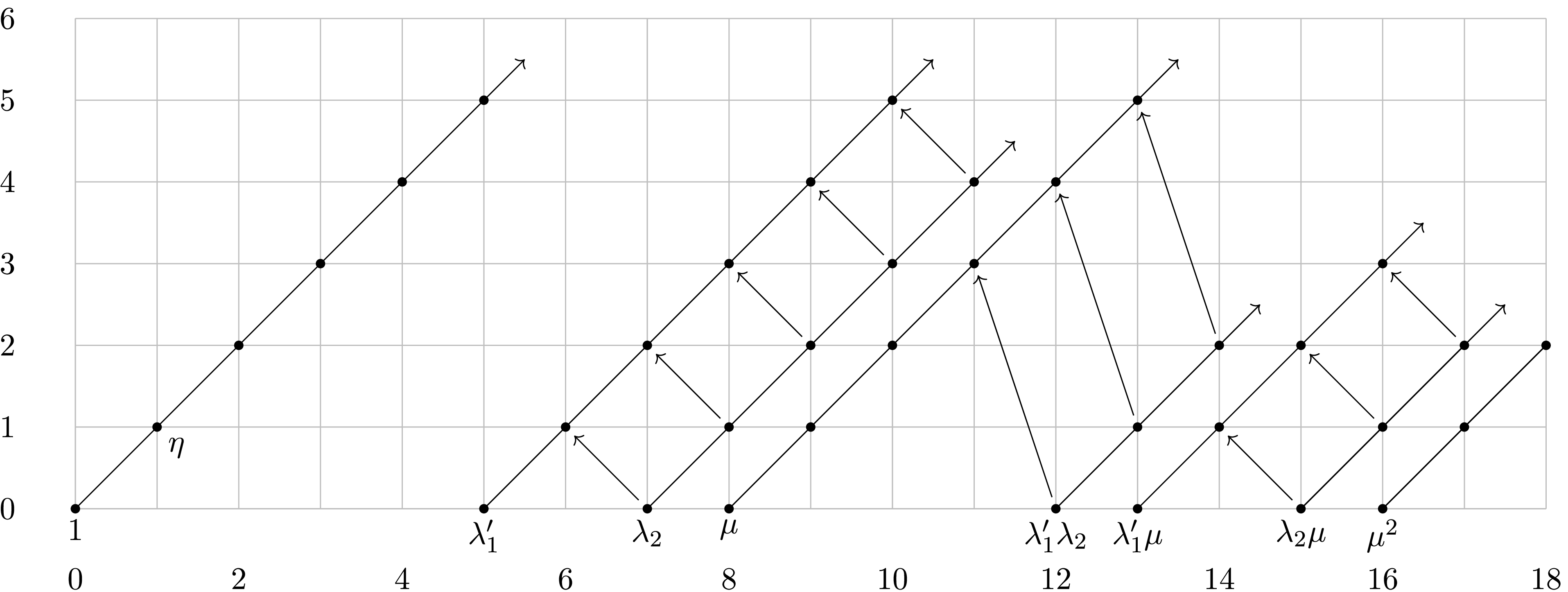
 F2[v2]
 (2,η,v1)
 −1
 1/3
 ∂
 η
 ν
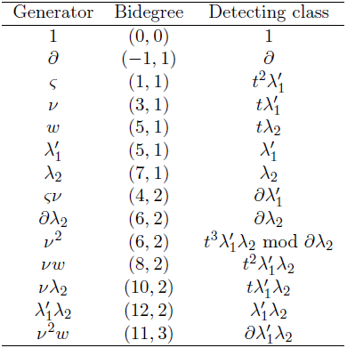
 F2[v2]
 A¯(1)∗grmot∗TC(ko)
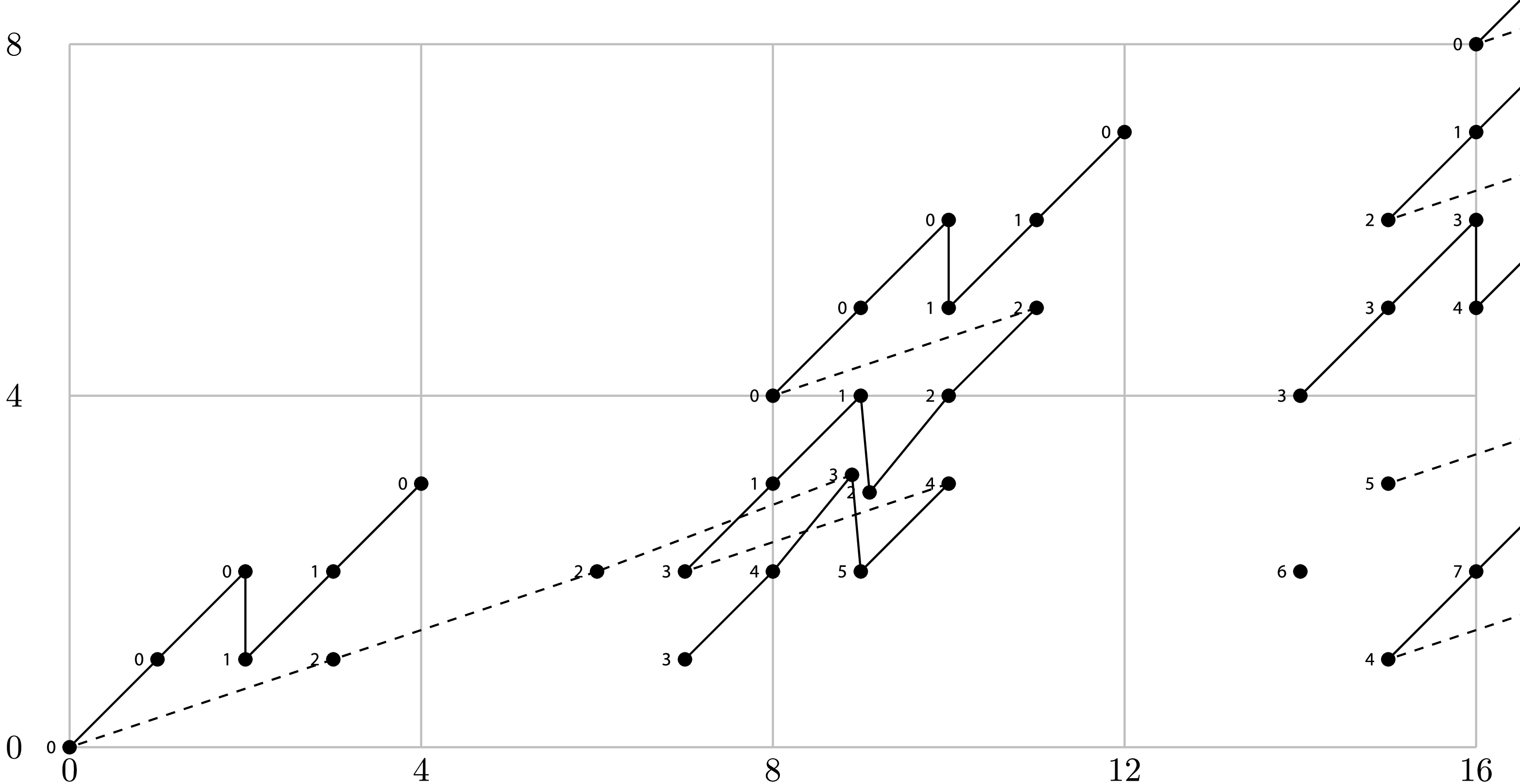
 η
 E1⟹V¯(1)∗grmot∗THH(ko)

 E2
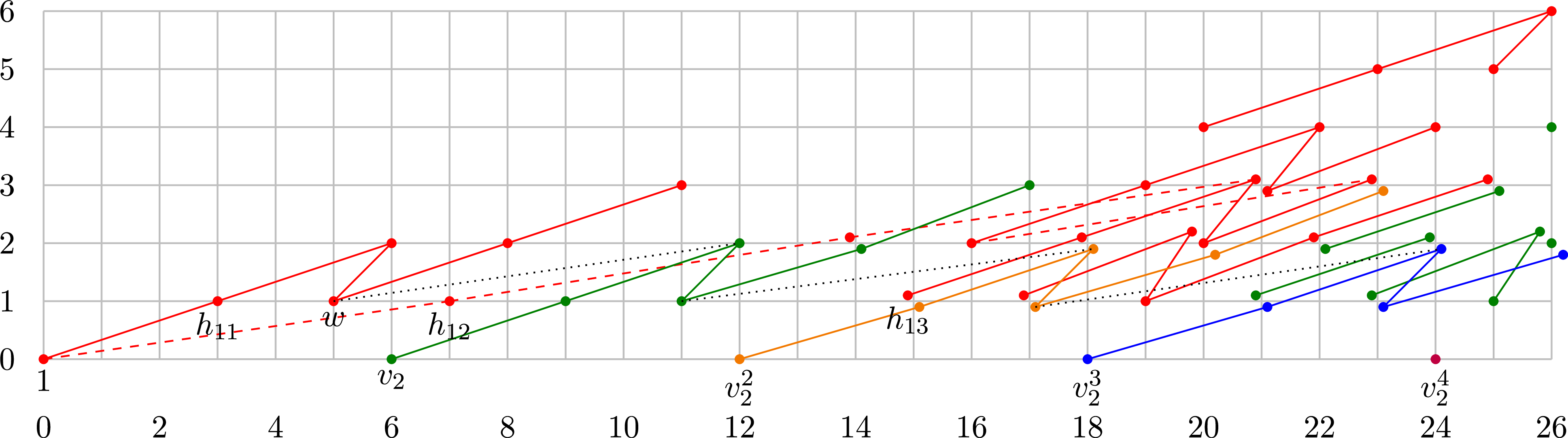
 v2
 E∞⟹ExtBP∗BP(BP∗,BP∗/I2)
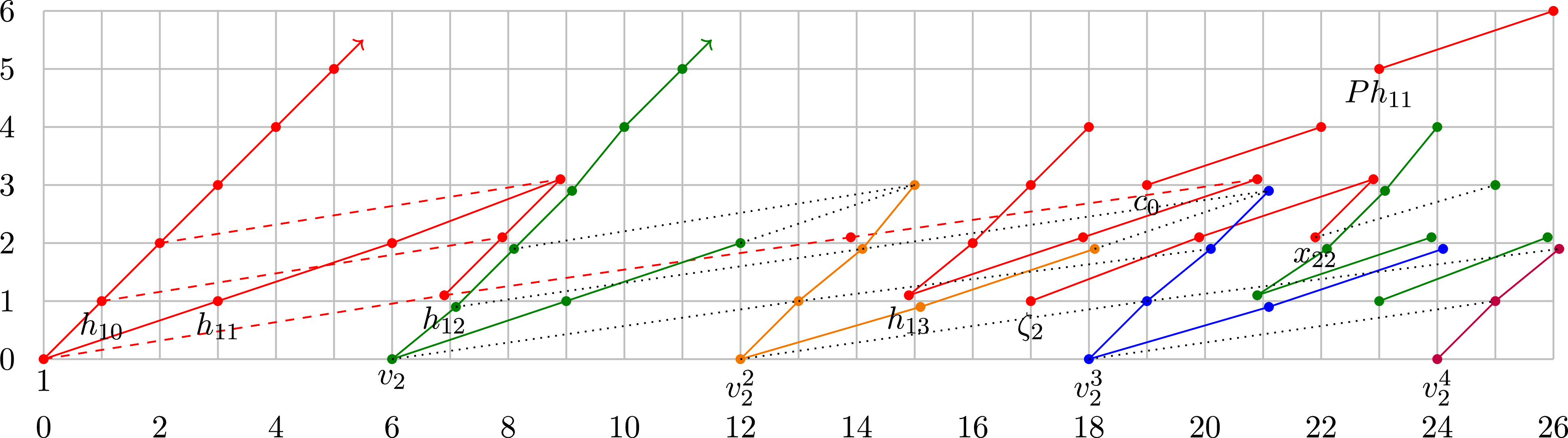
 E2
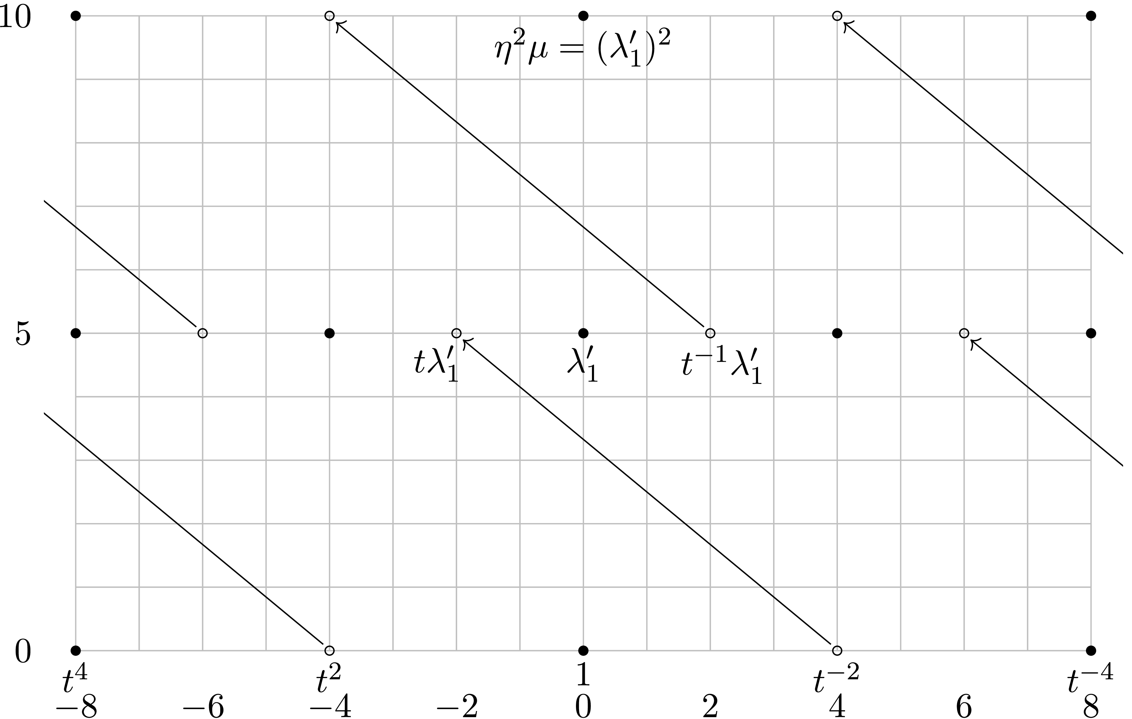
 v2
 E∞⟹ExtBP∗BP(BP∗,BP∗A(1))

 T
 E^4(T)⟹V¯(2)∗grmot∗TP(ko)

 T
 E^4(T)⟹(V¯(2)⊗C¯η)∗grmot∗TP(ko)

 T
 V¯(2)∗grmot∗TC−(ko)
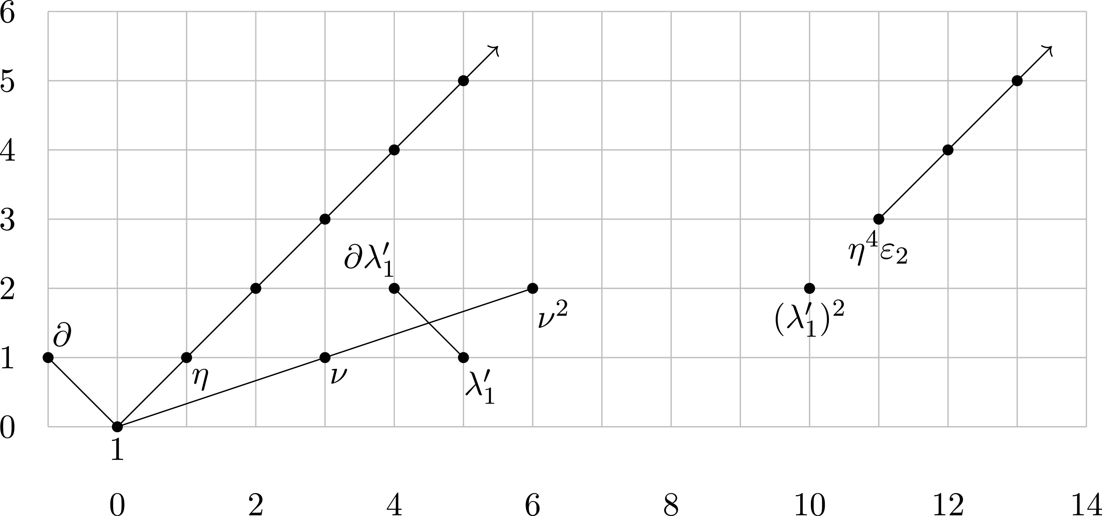
 T
 F2
 (V¯(2)⊗C¯η)∗grmot∗TC−(ko)

 F2
 V¯(2)∗grmot∗TC(ko)
 −1
 1/3
 ∂
 η
 ν

 v2
 E1⟹V¯(1)∗grmot∗TC(ko)

 F2[v2]
 A¯(1)∗grmot∗TC(ko)

 Open access

