








1 Introduction
The instability of a heavy fluid layer on top of a lighter one in a gravitational field was first studied by Rayleigh (Reference Rayleigh1883), and was later applied to accelerated frames by Taylor (Reference Taylor1950). Rayleigh found that small perturbations on the interface between the two fluids grow exponentially in time in the linear regime. Taylor’s analysis obtained the dispersion relationship for the inviscid instability, neglecting surface tension along the interface, and showed that the linearized equations apply for
 $ka\ll 1$
where
 $k$
is the wavenumber, and
 $a$
is the amplitude of the instability wave. Taylor’s result was then verified by Lewis (Reference Lewis1950) in his air/liquid experiments, in which he discovered that the bubble velocity approached a constant value after the linear stage. Few early studies explored the later stages of the Rayleigh–Taylor instability (RTI). However, the experimental studies of Ratafia (Reference Ratafia1973) and Popil & Curzon (Reference Popil and Curzon1979) studied the RTI into the nonlinear regime. Additionally, Layzer (Reference Layzer1955) developed a nonlinear model by solving for the velocity field near the bubble tip for
 $A=1$
, where
 $A$
is the Atwood number
 $A=(\unicode[STIX]{x1D70C}_{2}-\unicode[STIX]{x1D70C}_{1})/(\unicode[STIX]{x1D70C}_{2}+\unicode[STIX]{x1D70C}_{1})$
,
 $\unicode[STIX]{x1D70C}_{1}$
is the density of the light fluid, and
 $\unicode[STIX]{x1D70C}_{2}$
is the density of the heavy fluid. Layzer found that the bubbles approach a ‘terminal velocity’
 $$\begin{eqnarray}V_{b}\rightarrow \sqrt{\frac{gR}{3\unicode[STIX]{x03C0}}}\quad \text{as}~t\rightarrow \infty ,\end{eqnarray}$$
for Cartesian, two-dimensional (2-D) bubbles, where
 $R$
is the bubble radius, and
 $g$
is the acceleration of the interface.
Modern experiments have sought to extend our understanding of the RTI through the nonlinear regime, while the most recent experimental studies have focused on the late-time turbulent development and mixing (Andrews & Dalziel Reference Andrews and Dalziel2010). There have been relatively few experiments exploring the 3-D, single-mode instability, with the exception of Jacobs & Catton (Reference Jacobs and Catton1988) who studied square mode and cylindrical 3-D perturbations, Wilkinson & Jacobs (Reference Wilkinson and Jacobs2007) who studied moderate Atwood number incompressible systems and Dimonte, Gore & Schneider (Reference Dimonte, Gore and Schneider1998) who studied elastic–plastic materials. Additionally, there have been relatively few gas phase RTI experiments. Banerjee & Andrews (Reference Banerjee and Andrews2006) extended the Texas A&M water channel experiment to larger Atwood numbers by the use of a gas channel apparatus, and Zaytsev et al. (Reference Zaytsev, Krivets, Mazilin, Titov, Chebotareva, Nikishin, Tishkin, Bouquet and Haas2003) developed a gas phase experiment that used compression waves generated by a combustible mixture to shocklessly accelerate interfaces. The compressible experiments of Zaytsev et al. (Reference Zaytsev, Krivets, Mazilin, Titov, Chebotareva, Nikishin, Tishkin, Bouquet and Haas2003) generated RTI growth, but exhibited additional effects due to compressibility.
The advent of high-speed computing has enabled the numerical solution of numerous problems related to the RTI, including the numerical simulations of Ramaprabhu & Dimonte (Reference Ramaprabhu and Dimonte2005), who used 3-D numerical simulations to study the development of the single-mode RTI into the nonlinear regime. These numerical simulations have shown good agreement with the extended Layzer model of Goncharov (Reference Goncharov2002), which included the effects of the Atwood number, and the Lagrangian buoyancy–drag model of Oron et al. (Reference Oron, Arazi, Kartoon, Rikanati, Alon and Shvarts2001). Both of these models suggest
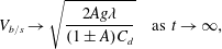 $$\begin{eqnarray}V_{b/s}\rightarrow \sqrt{\frac{2Ag\unicode[STIX]{x1D706}}{(1\pm A)C_{d}}}\quad \text{as}~t\rightarrow \infty ,\end{eqnarray}$$
where
 $C_{d}=6\unicode[STIX]{x03C0}$
for two dimensions, and
 $C_{d}=2\unicode[STIX]{x03C0}$
for 3-D asymptotic bubble (
 $+$
sign) and spike (
 $-$
sign) velocities.
Ramaprabhu et al. (Reference Ramaprabhu, Dimonte, Young, Calder and Fryxell2006) also showed that bubble and spike terminal velocities can be expressed dimensionlessly as a Froude number
 $$\begin{eqnarray}Fr_{b/s}=V_{b/s}\left(\frac{g\unicode[STIX]{x1D706}A}{1\pm A}\right)^{-1/2},\end{eqnarray}$$
where
 $\unicode[STIX]{x1D706}$
is the wavelength of the interface perturbation. Thus, the results of Goncharov and Oron yield
 $Fr_{b/s}\rightarrow 1/\sqrt{3\unicode[STIX]{x03C0}}$
for two dimensions, and
 $Fr_{b/s}\rightarrow 1/\sqrt{\unicode[STIX]{x03C0}}$
for three dimensions as
 $t\rightarrow \infty$
.
Glimm & Li (Reference Glimm and Li1988) used simulations to validate a bubble merger model, and showed that compressibility affects the bubble late-time velocity Froude number. Their results indicate that the bubble late-time velocity Froude number is a monotonically increasing function of
 $$\begin{eqnarray}G=\sqrt{\frac{g}{k{a_{s}}^{2}}},\end{eqnarray}$$
where
 $a_{s}$
is the sound speed of the surrounding fluid (Sharp Reference Sharp1984; Glimm & Li Reference Glimm and Li1988). Mikaelian (Reference Mikaelian2009) further extended the Layzer model to account for time varying densities and accelerations, which resulted in a pair of coupled ordinary differential equations (ODEs),
 $$\begin{eqnarray}\frac{\text{d}}{\text{d}t}(\unicode[STIX]{x1D70C}_{2}\unicode[STIX]{x1D702}_{2})=-\frac{ck}{4}\left[k+\frac{4(1+c)}{c}\,\unicode[STIX]{x1D702}_{2}\right]\frac{\text{d}}{\text{d}t}(\unicode[STIX]{x1D70C}_{2}\unicode[STIX]{x1D702}),\end{eqnarray}$$
 $$\begin{eqnarray}\displaystyle & & \displaystyle \unicode[STIX]{x1D70C}_{2}\left\{\frac{ck}{4}\,\frac{\text{d}}{\text{d}t}\left[\frac{1}{\unicode[STIX]{x1D70C}_{2}}\,\frac{\text{d}}{\text{d}t}(\unicode[STIX]{x1D70C}_{2}\unicode[STIX]{x1D702})\right]+\frac{c^{2}k^{2}}{8}\left[\frac{1}{\unicode[STIX]{x1D70C}_{2}}\frac{\text{d}}{\text{d}t}(\unicode[STIX]{x1D70C}_{2}\unicode[STIX]{x1D702})\right]^{2}\right\}\nonumber\\ \displaystyle & & \displaystyle \qquad +\,\unicode[STIX]{x1D70C}_{1}\left\{\frac{ck}{4}\,\dot{b_{1}}-\frac{c^{2}k^{2}}{8}\,b_{1}^{2}\right\}+(\unicode[STIX]{x1D70C}_{2}-\unicode[STIX]{x1D70C}_{1})(g+\ddot{\unicode[STIX]{x1D702}})\unicode[STIX]{x1D702}_{2}=0,\end{eqnarray}$$
where
 $$\begin{eqnarray}b_{1}=\left.\left[\frac{1}{k\unicode[STIX]{x1D70C}_{1}}\,\frac{\text{d}}{\text{d}t}(\unicode[STIX]{x1D70C}_{1}\unicode[STIX]{x1D702}_{2})\right]\right/\left[(1+c)\unicode[STIX]{x1D702}_{2}-\frac{ck}{4}\right],\end{eqnarray}$$
 $\unicode[STIX]{x1D702}$
is the amplitude of the perturbation,
 $\unicode[STIX]{x1D702}_{2}$
relates to the curvature of the interface,
 $c=1$
for axisymmetric perturbations and
 $c=2$
for 2-D Cartesian perturbations. The bubble velocities given by these types of models have produced good agreement with experiments and simulations. However, according to Mikaelian (Reference Mikaelian2008) the model fails for spikes. It is theorized that at large Atwood numbers, spikes will free fall (Baker, Meiron & Orszag Reference Baker, Meiron and Orszag1980; Menikoff & Zemach Reference Menikoff and Zemach1983; Zhang Reference Zhang1998), i.e.
 $a\propto z$
, where
 $z=gt^{2}/2$
is the interface displacement in the direction of acceleration (gravity). Additionally, Baker et al. (Reference Baker, Meiron and Orszag1980) and Dimonte (Reference Dimonte1999) proposed that ensembles of spikes in free fall will grow as
 $Az$
. Models for the nonlinear development of the spike have proven difficult to formulate, with current versions only describing
 $A=1$
behaviour (Clavin & Williams Reference Clavin and Williams2005), or interpolating between
 $A=1$
(free fall) and
 $A=0$
(‘terminal velocity’) behaviours (Mikaelian Reference Mikaelian2014).
More recently, Ramaprabhu et al. (Reference Ramaprabhu, Dimonte, Woodward, Fryer, Rockefeller, Muthuraman, Lin and Jayaraj2012) and Wei & Livescu (Reference Wei and Livescu2012) showed that 3-D single-mode bubble and spike velocities do not remain at a ‘terminal velocity’, but rather reaccelerate in a process described by Ramaprabhu et al. (Reference Ramaprabhu, Dimonte, Woodward, Fryer, Rockefeller, Muthuraman, Lin and Jayaraj2012) as leading to ‘chaotic mixing’ which may eventually lead to a turbulent state. According to Ramaprabhu et al. (Reference Ramaprabhu, Dimonte, Woodward, Fryer, Rockefeller, Muthuraman, Lin and Jayaraj2012), this reacceleration occurs at the onset of secondary Kelvin–Helmholtz (KH) instability, leading to an unstable bubble velocity plateau. This reacceleration is described as a process similar to that described by Betti & Sanz (Reference Betti and Sanz2006), where vorticity accumulates in the bubble and alters its dynamics. Wei & Livescu (Reference Wei and Livescu2012) propose a different mechanism, where ‘chaotic development’ and reacceleration are the consequence of complex, but symmetry preserving, vortical interactions. Furthermore, reacceleration was observed by Reckinger, Livescu & Vasilyev (Reference Reckinger, Livescu and Vasilyev2010) in 2-D simulations, and was shown to occur in 3-D experiments by Wilkinson & Jacobs (Reference Wilkinson and Jacobs2007) who produced Froude number trends comparable to Ramaprabhu et al. (Reference Ramaprabhu, Dimonte, Young, Calder and Fryxell2006).
Of the few experiments previously reported, none have studied the single-mode, nonlinear, gas phase Rayleigh–Taylor instability. In this study we will generate gas phase, Rayleigh–Taylor unstable interfaces by using the acceleration provided by a rarefaction wave. The rarefaction wave generates a large but non-constant acceleration, and results in time varying densities (and time varying Atwood numbers). The early time, linearized growth rate of these interfaces was considered in Morgan, Likhachev & Jacobs (Reference Morgan, Likhachev and Jacobs2016). Herein, the role of variable acceleration and density during the nonlinear development of the instability will be explored. This will be accomplished by comparison of experiments with numerical simulations, incompressible models and variable density models.
2 Experimental apparatus and procedure
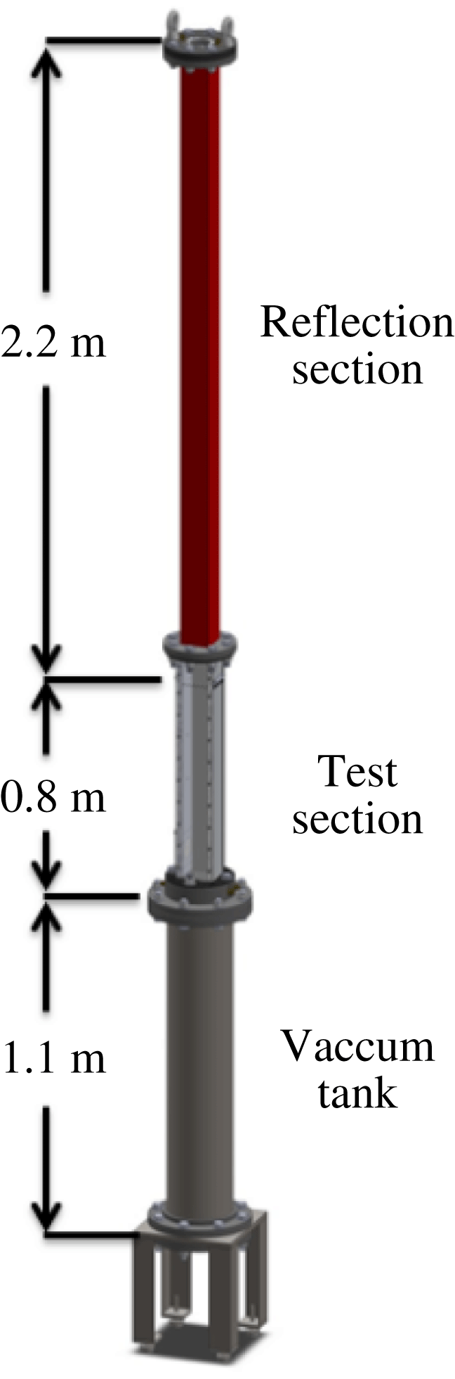
Figure 1 shows the rarefaction tube that the experiments in this study were performed in. This apparatus consists of a vertical hollow tube in which an interface is generated using the membraneless, counterflow technique of Jones & Jacobs (Reference Jones and Jacobs1997). The rupturing of a diaphragm launches a rarefaction wave upward toward the interface, imparting a large downward acceleration on the interface (Morgan et al.
Reference Morgan, Likhachev and Jacobs2016). The bottom of the apparatus is a vacuum tank that is 1.1 m long. The test section is 80.6 cm long, has a square cross-section with width
 $W=88.9$
mm, and is separated from the vacuum tank by the heavy gas plenum which sits directly above the diaphragm. The heavy gas plenum has a height of 5.4 cm, and the resulting distance from the diaphragm location to the interface generation holes is 76.6 cm. The test section has two 19.0 mm thick aluminium sides with an 11.2 mm thick clear acrylic front, and a black or clear acrylic back. These faces have 6 small 2.3 mm holes that allow the test gases to escape and form a diffuse interface. Two PCB Piezotronics 112A21 pressure transducers mounted on one side of the test section at 34.1 cm and 18.8 cm below the interface generation holes, are used to record the pressure history of the experiments, and provide trigger signals to start image acquisition. The reflection section is comprised of a 2.07 m long section of square fiberglass tube, resulting in a distance of 2.18 m to the top wall from the interface. The top of the reflection section is enclosed with a flange, where a 76 mm diameter fused silica window, and two light gas inlets are attached.
Experiments were initiated by flowing a light gas from the top of the apparatus, and a heavy gas from the bottom of the test section. Matched volumetric flow rates of
 $6~\text{l}~\text{min}^{-1}$
were used to generate a flat diffuse interface at the small holes near the top of the test section. The interface was observed during this interface generation process, and once the interface had stabilized, a vacuum pump evacuated the vacuum tank. Prior to the experiment, the pressure in the test section is assumed to be the local atmospheric pressure of approximately
 $93.2$
kPa. When the pressure in the vacuum tank dropped below
 $2.03$
kPa, oscillatory forcing was started.
Nearly 2-D single-mode perturbations were generated by rocking the apparatus side-to-side in the imaged plane using a method developed for single-mode shock tube experiments (Jones & Jacobs Reference Jones and Jacobs1997; Collins & Jacobs Reference Collins and Jacobs2002; Jacobs & Krivets Reference Jacobs and Krivets2005). This motion caused 2-D standing waves to form in the test section. Note that the experiments are of course not purely two-dimensional, but the terminology two-dimensional will herein refer to experiments with 2-D initial perturbations. The rocking was generated by an Isel Electronics
 $1.8^{\circ }$
/step A2537-9212-A1 stepper motor that is mounted to the ceiling of the dark room in which the apparatus is located. The phase of oscillation was used to determine a time delay such that the rarefaction wave arrived when the optimum interface perturbation was present. Table 1 shows the forcing frequencies and amplitudes used to generate the 2-D perturbations. Additionally, the front and rear interface generation holes were sealed to produce 2-D perturbations.
A schematic representation of the rarefaction tube showing the locations and lengths of the three main regions of the apparatus. These regions include the vacuum tank which is initially separated from the test section by a diaphragm, the test section which is initially filled with heavy gas up to the interface generation holes, and the reflection section which is initially filled with light gas. Dimensions are given to the interface generation holes and hence represent the extents of the light and heavy gas regions.
Forcing amplitudes
 $a_{f}$
, and frequencies
 $\unicode[STIX]{x1D714}$
used to generate nominally 2-D waves in the test section for each of the gas pairs and wavenumbers used.

Single-mode 3-D perturbations were generated using a Tang Band W5-1138SM loudspeaker attached near the bottom of the test section that vertically oscillated the column of gas. During this oscillation, the interface generation holes on all four sides were left open. The oscillation waveform and a synchronization pulse were generated using an Agilent U2531A digital input/output board. The speakers were driven sinusoidally at a fixed frequency during each of the experiments. This leads to a 3-D perturbation, the form of which is given in more detail in § 3. Table 2 lists the frequencies and amplitudes applied for 3-D single-mode perturbations.
When the pressure dropped below
 $1.01$
kPa, a trigger pulse initiated the experiment, sending a signal to the solenoid that burst the diaphragm using an attached arrowhead. When the lower pressure transducer signal dropped
 $2.74$
kPa below ambient, indicating the arrival of the leading edge of the rarefaction wave, image acquisition using the DaVis software from Lavision was initiated. The goal of this diaphragm puncturing is to cause the head of a rarefaction wave to travel into the test section, while the tail remains centred at the diaphragm location (or extends into the vacuum tank). This rarefaction wave configuration requires sonic conditions at the diaphragm location. Note, however, that it is very difficult in practice to create sonic conditions at the diaphragm location, as small variations in the cross-section area can cause the Mach number there to drop below unity (Owczarek Reference Owczarek1964).
A Mie scattering diagnostic was employed to visualize a thin slice of the mixing region over time. Incense smoke from a single stick of incense, was seeded in a coaxial flow of 0.6
 $\text{l}~\text{min}^{-1}$
of air and then mixed with the heavy gas flowing at 5.4
 $\text{l}~\text{min}^{-1}$
. The laser illuminated Mie scattering set-up is described in Morgan et al. (Reference Morgan, Likhachev and Jacobs2016). The laser sheet expands downward to the interface, illuminating it from the top. Experiments studying the nonlinear development of the RTI were conducted using a wide angle 28 mm camera lens to view the entire test section. Diagonal planes of the 3-D interface were visualized by rotating the laser sheet by
 $45^{\circ }$
, and using a perspective correction in DaVis that employed a calibration plate placed diagonally in the test section prior to experiments.
Forcing frequencies
 $\unicode[STIX]{x1D714}$
, and amplitudes
 $a_{f}$
for
 $\text{CO}_{2}\text{/}\text{SF}_{6}$
and
 $\text{air}\text{/}\text{SF}_{6}$
3-D single-mode experiments. The value of
 $a_{f}$
(V) root-mean-square (r.m.s.) meas. is taken after amplification.

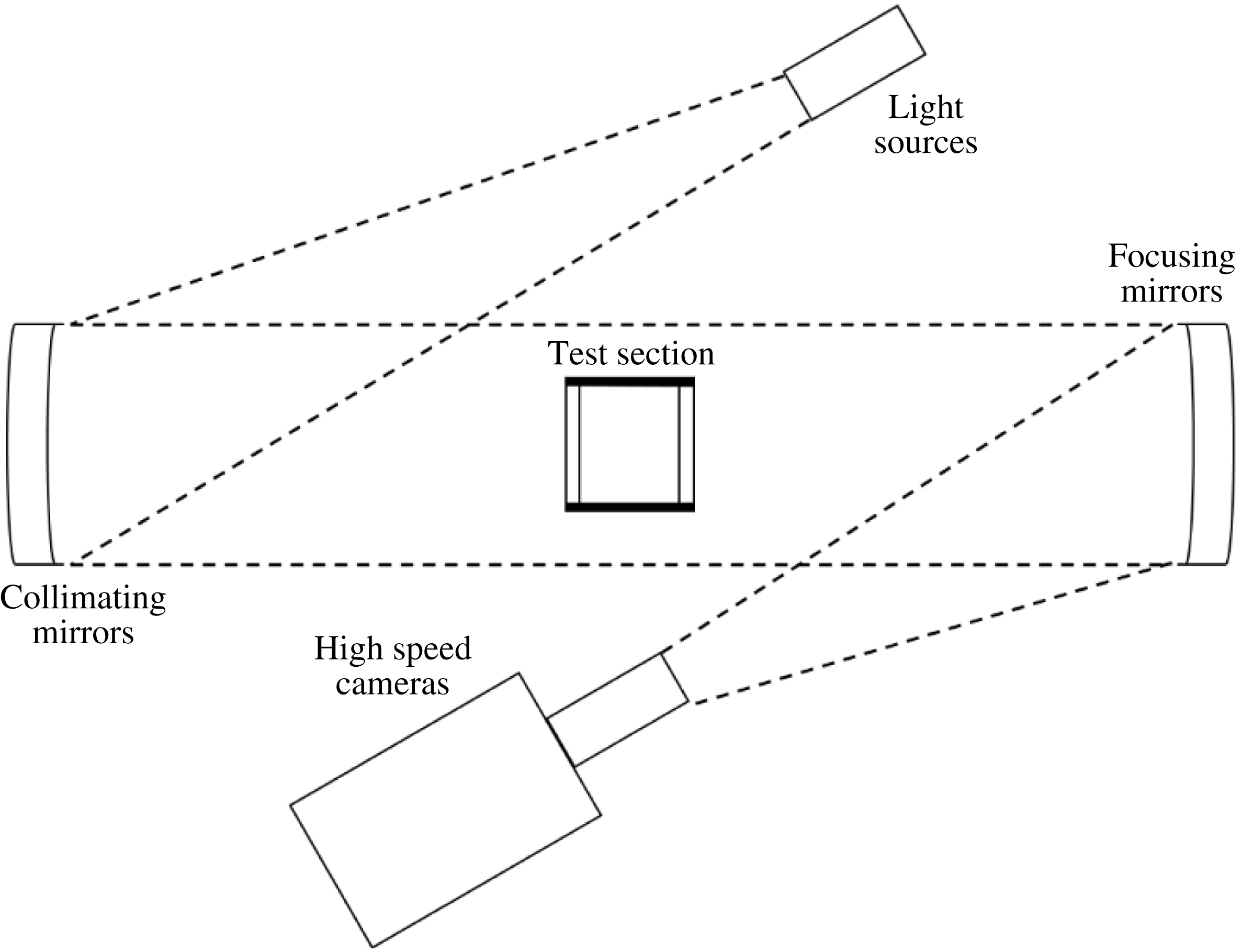
In addition to Mie scattering, figure 2 shows a shadowgraph system that was used to visualize the instability. High-powered LedEngin LZ4-40NW00 white light emitting diodes (LEDs) were chosen for this system due to their small element size, which minimizes geometric blur, and broadband output, which smooths interference fringing (Settles Reference Settles2001). Light from the three LEDs is first collimated using three 200 mm aperture f/6 parabolic telescope mirrors, and then travels through the test section which has a clear front and back, where it is distorted by the density gradients at the interface. This distorted light is then collected by another set of three 200 mm aperture f/6 parabolic telescope mirrors, which focus light through three 105 mm focal length, f/2.8 camera lenses onto the sensors of three high-speed CMOS cameras operating at 6 kHz. These optical paths are in the schlieren Z shape to minimize distortions (Settles Reference Settles2001). This set-up is capable of visualizing 3-D density disturbances, and can be used to visualize the instability without seeding. This visualization technique produces an integrated view of the development of the RTI, but is obscured by the presence of boundary layers, and hence is not used for quantitative comparison.
A schematic of the shadowgraph system developed to visualize waves (rarefactions and compressions) and interfaces in the rarefaction tube. The light from high-powered LEDs is collimated by a set of parabolic mirrors which direct the light through the test section. Another set of parabolic mirrors collect the light and focus it onto the sensors of three high-speed CMOS cameras.
3 Miranda code
Simulations were computed using the compressible research hydrodynamics code Miranda, developed at Lawrence Livermore National Laboratory (LLNL). The compressible version of the Miranda code (Cook & Cabot Reference Cook and Cabot2004, Reference Cook and Cabot2005; Cook Reference Cook2007) solves the Navier–Stokes equations for compressible ideal gases with constant specific heats. Notably, this code includes the diffusion of enthalpy (Cook Reference Cook2009), a process that is often neglected. In order to capture the effects of small scales on the problem, grid-dependent artificial viscosities and diffusivities are used. This method is termed artificial fluid large eddy simulation (AFLES). The governing equations are computed using a fourth-order Runge–Kutta scheme in time, a tenth-order compact finite difference scheme for non-periodic spatial derivatives and Fourier transforms for spatially periodic derivatives (Cook & Cabot Reference Cook and Cabot2005; Cook Reference Cook2007).
Problems are solved on a Cartesian grid denoted by
 $x$
running from left to right,
 $y$
running into the page and
 $z$
running from bottom to top. Two-dimensional simulations are conducted in the
 $x$
–
 $z$
plane, while for all simulations the mean flow travels in the
 $-z$
direction. In the
 $x$
and
 $y$
directions 256 points are used, while in the
 $z$
direction, the resolution depends on the wavelength of the perturbations used. The domain is one wavelength wide in the
 $x$
and
 $y$
directions, and extends from the origin of the rarefaction wave to one wavelength beyond the interface at
 $z_{i}(t=0)=76.6$
cm from the bottom boundary. The top and bottom boundary conditions are set to ‘free’, a characteristic boundary condition that lets rarefaction waves and material in and out (Thompson Reference Thompson1987; Poinsot & Lele Reference Poinsot and Lele1992). In the horizontal directions, the boundary conditions are periodic. One perturbation wavelength is imposed at the interface with an error function diffusion profile in the vertical direction.
The rarefaction wave is initialized as a centred isentropic rarefaction with origin at the bottom boundary. It can easily be shown that the sound speed will vary through a rarefaction wave travelling in the positive
 $z$
direction as
 $$\begin{eqnarray}a_{s}=\frac{2a_{s}(0)}{\unicode[STIX]{x1D6FE}+1}+\frac{\unicode[STIX]{x1D6FE}-1}{\unicode[STIX]{x1D6FE}+1}\,\frac{z}{t},\end{eqnarray}$$
where
 $a_{s}$
is the speed of sound in the heavy gas,
 $a_{s}(0)$
is the initial speed of sound in the heavy gas and
 $\unicode[STIX]{x1D6FE}$
is the adiabatic index of the heavy gas. In order to save computational time, the rarefaction wave is propagated to a position
 $z_{wave}$
at time
 $t_{wave}$
. The head of the rarefaction wave travelling at the speed of sound in the heavy gas arrives at
 $t_{wave}=z_{wave}/a_{s}(0)$
. Thus the sound speed can be expressed as a function of
 $z$
at time
 $t_{wave}$
as
 $$\begin{eqnarray}a_{s}=a_{s}(0)\left(\frac{2}{\unicode[STIX]{x1D6FE}+1}+\frac{\unicode[STIX]{x1D6FE}-1}{\unicode[STIX]{x1D6FE}+1}\,\frac{z}{z_{wave}}\right).\end{eqnarray}$$
The velocity can then be set as
 $$\begin{eqnarray}u=\frac{z}{t_{wave}}-a_{s},\end{eqnarray}$$
and thermodynamic variables are set using the isentropic relations. For example, density, pressure and temperature are set as
 $$\begin{eqnarray}\displaystyle & \displaystyle \unicode[STIX]{x1D70C}=\unicode[STIX]{x1D70C}_{0}\left(\frac{a_{s}}{a_{s}(0)}\right)^{2/(\unicode[STIX]{x1D6FE}-1)}, & \displaystyle\end{eqnarray}$$
 $$\begin{eqnarray}\displaystyle & \displaystyle p=p_{0}\left(\frac{a_{s}}{a_{s}(0)}\right)^{2\unicode[STIX]{x1D6FE}/(\unicode[STIX]{x1D6FE}-1)}, & \displaystyle\end{eqnarray}$$
 $$\begin{eqnarray}\displaystyle & \displaystyle T=T_{0}\left(\frac{a_{s}}{a_{s}(0)}\right)^{2}, & \displaystyle\end{eqnarray}$$
where
 $\unicode[STIX]{x1D70C}_{0}$
is the initial heavy gas density,
 $p_{0}$
is the initial pressure and
 $T_{0}$
is the initial temperature. Initial temperature and pressure values of
 $T_{0}=297.04$
K and
 $p_{0}=93.22$
kPa are used. Figure 3 shows the initial density distribution from an
 $\text{air}\text{/}\text{SF}_{6}$
simulation. The positions of the head of the rarefaction wave, the interface and boundaries can be seen. Note that the rarefaction wave causes a spatially varying density distribution where the bubbles will travel into regions of lower density fluid. This is very different from classical RTI simulations with uniform background density from isothermal initial conditions (Reckinger, Livescu & Vasilyev Reference Reckinger, Livescu and Vasilyev2016). Simulations are initiated with the head of the rarefaction wave one perturbation wavelength below the interface. When the simulations start, the wave travels upward toward the stationary interface and induces a downward motion. The simulation is terminated when the light gas region (bubble) reaches the bottom boundary. Identical simulations were run without perturbations in order to separate bubbles and spikes. Perturbations are input as one wavelength of a cosine wave such that the 50 % concentration contour is given by
 $$\begin{eqnarray}\unicode[STIX]{x1D702}(x)=z_{i}-a_{0}\cos \left(\frac{2n_{x}\unicode[STIX]{x03C0}x}{W}\right)\end{eqnarray}$$
for two dimensions, and
 $$\begin{eqnarray}\unicode[STIX]{x1D702}(x,y)=z_{i}+\frac{a_{0}}{2}\left[\cos \left(\frac{2n_{x}\unicode[STIX]{x03C0}x}{W}\right)+\cos \left(\frac{2n_{y}\unicode[STIX]{x03C0}y}{W}\right)\right]\end{eqnarray}$$
for three dimensions. Here,
 $z_{i}$
is the mean location of the interface,
 $a_{0}$
is the initial amplitude of the perturbation,
 $n_{x}$
is the number of perturbation wavelengths in the
 $x$
direction and
 $n_{y}$
is the number of perturbation wavelengths in the
 $y$
direction. The interface is made diffuse by applying an error function to the
 $50\,\%$
concentration contour of the heavy gas
 $$\begin{eqnarray}X_{2}(x,y,z)=\frac{1}{2}\left[1+\text{erf}\left(\sqrt{\unicode[STIX]{x03C0}}\,\frac{z-\unicode[STIX]{x1D702}}{\unicode[STIX]{x1D6FF}}\right)\right],\end{eqnarray}$$
where
 $X_{2}$
is the volume fraction of the heavy gas,
 $X_{1}=1-X_{2}$
and
 $X_{1}$
is the volume fraction of light gas.
The initial distribution of density in a 2-D
 $\text{air}\text{/}\text{SF}_{6}$
simulation which shows the single-mode 2-D perturbation (a), the location of the interface (b) and the location of the rarefaction wave (b). Simulations are started with the rarefaction wave one wavelength below the interface.

4 Ares code
Ares is an arbitrary Lagrange Eulerian (ALE) hydrodynamics code developed at LLNL (McFarland, Greenough & Ranjan Reference McFarland, Greenough and Ranjan2011). The Lagrange time advancement is second-order predictor–corrector and uses the Gauss divergence theorem to give the discrete finite difference equations (Wilkins Reference Wilkins1963). The Lagrange scheme operates on a staggered mesh where velocities are defined at nodes and the density and energy are defined at zone centres. All numerical differences are fully second order in space. Artificial viscosity is used to suppress spurious oscillations following the method of Kolev & Rieben (Reference Kolev and Rieben2009). The remap phase of the calculation, where the Lagrangian solution is remapped back to a non-Lagrangian mesh, is fully second order. The original method is given by Sharp & Barton (Reference Sharp and Barton1981).
The Ares code was used extensively in this study to model the flow in the rarefaction tube under a variety of conditions. These 1-D, 2-D and axisymmetric simulations were used to guide the design of the rarefaction tube prior to construction. Results from a two-dimensional and an axisymmetric simulation will be shown in § 7.1 and § 7.2, respectively. Here axisymmetric means that the simulations are conducted in cylindrical coordinates where properties are constant in the azimuthal direction. Thus, the square cross-section becomes a cylinder with a diameter equal to the width of the apparatus. This choice represents the inscribed case which is chosen due to its simple set-up and equivalent hydraulic diameter
 $D_{h}=4A_{x}/P$
, where
 $A_{x}$
is the cross-sectional area, and
 $P$
is the perimeter.
The initial perturbation was input into Ares in a manner identical to Miranda using (3.7) and (3.9), with only one half-wavelength simulated. The initial conditions were input in a very different manner than in Miranda. The entire rarefaction tube was simulated using a base resolution of 1350 points in the vertical direction. Four levels of refinement by a factor of 3 were applied on the Laplacian of density resulting in a transverse resolution of approximately 400–500 points per wavelength. That is, each time the refinement criterion is met in a cell, the edge length of the cell is divided by three. This process is repeated a maximum of four times. This caused the mesh to be refined near the interface, and near the head of the rarefaction wave. The rarefaction wave was not input directly as an initial condition in Ares, but rather, the initial pressure jump across the diaphragm was used. At the initial time, the rarefaction wave forms and travels toward the interface, much like in the experiment. All of the boundary conditions for the 2-D Ares simulations were input as 1-D reflecting boundaries. For the axisymmetric simulations, one of the 1-D reflecting boundary conditions was omitted and was set as the axis. Two simulations using
 $\text{air}\text{/}\text{SF}_{6}$
were run, one with an axisymmetric bubble, and one with an axisymmetric spike (where the bubble and spike designations imply that the axis of symmetry travels through the centre of the bubble and spike, respectively).
5 Image analysis
Two-dimensional experiments were analysed by tracking the point with the steepest intensity gradient in the vicinity of the bubble and spike tip in digital images of the experiments. World coordinates were determined from pixel positions by recording an image of a calibration plate that was placed in the plane of the laser sheet. Separate experiments were conducted for 3-D bubbles and spikes to minimize wall effects on the development of the instability. For 3-D experiments, the point with the steepest intensity gradient in the vicinity of the bubble tip for bubble experiments, or the spike tip for spike experiments, and the wall saddle points for both types of experiments were tracked.
Bubble and spike amplitudes were obtained in 2-D experiments by comparison with flat interface experiments conducted under identical conditions. Since these experiments experience a slight timing jitter due to inconsistencies in the rupturing of the diaphragm, comparison of bubble and spike experiments requires putting the bubble, spike and flat interface experiments on the same time basis relative to the initial acceleration time, referred to here as time aligning. This time alignment was conducted by comparing the interface displacement from the unperturbed flat interface experiment to the average of the bubble and spike displacements from the perturbed experiment at early time. The flat interface positions were then interpolated to the perturbed experimental times. Finally, the spike amplitude
 $a_{s}(t)=z_{s}(t)-z_{i}(t)$
, and the bubble amplitude
 $a_{b}(t)=z_{i}(t)-z_{b}(t)$
were calculated, where
 $z_{i}$
,
 $z_{s}$
and
 $z_{b}$
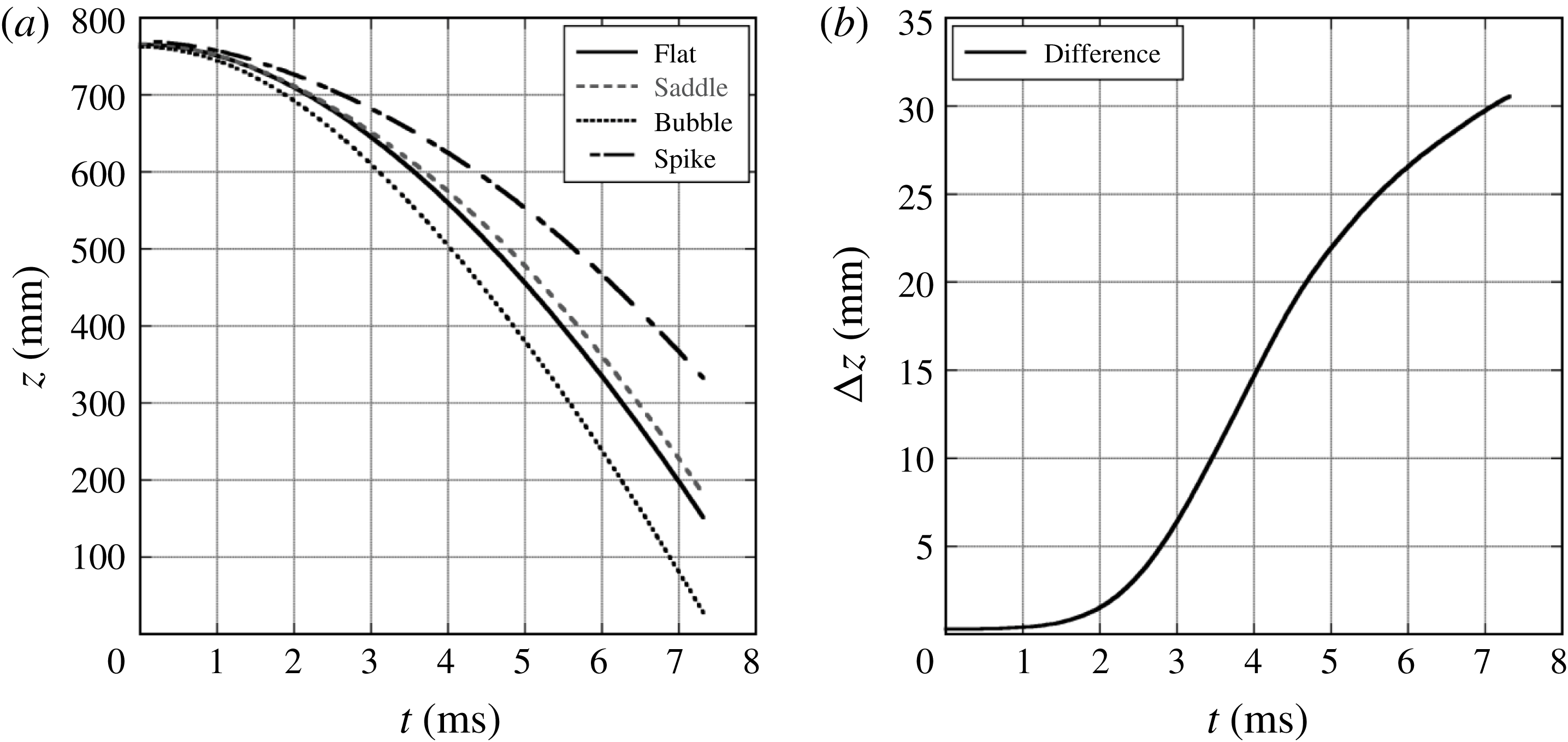
are the locations of the flat interface, spike and bubble, respectively. Figure 4 shows that the flat interface and average bubble and spike displacements are nearly equal at early times in simulations, motivating this approach.
The displacement of the bubble, spike, average of bubble and spike and flat interface locations from a 2-D 1.5 wavelength
 $\text{air}\text{/}\text{SF}_{6}$
Miranda simulation (a). At early times, the flat interface and average displacements are similar, and little error is introduced by matching the flat interface location to the average perturbed interface location (b).

Three-dimensional bubbles and spikes were obtained in a similar fashion as was done for the 2-D experiments, by the comparison with flat interface experiments. The perturbed experiments and unperturbed flat interface experiments were time aligned using the interface displacement from the unperturbed interface experiment, and the displacement of the saddle point for the perturbed experiment at early time. The flat interface positions were then interpolated to the perturbed experiment times. Figure 5 shows that the flat interface displacement and the saddle point displacement are in good agreement at early times in simulations.
The displacement of the bubble, spike, saddle and flat interface locations from a 3-D, 1.0 wavelength
 $\text{air}\text{/}\text{SF}_{6}$
Miranda simulation (a). At early times, the flat interface and saddle point displacements are similar, and the flat interface displacement can be matched to the saddle point displacement (b).
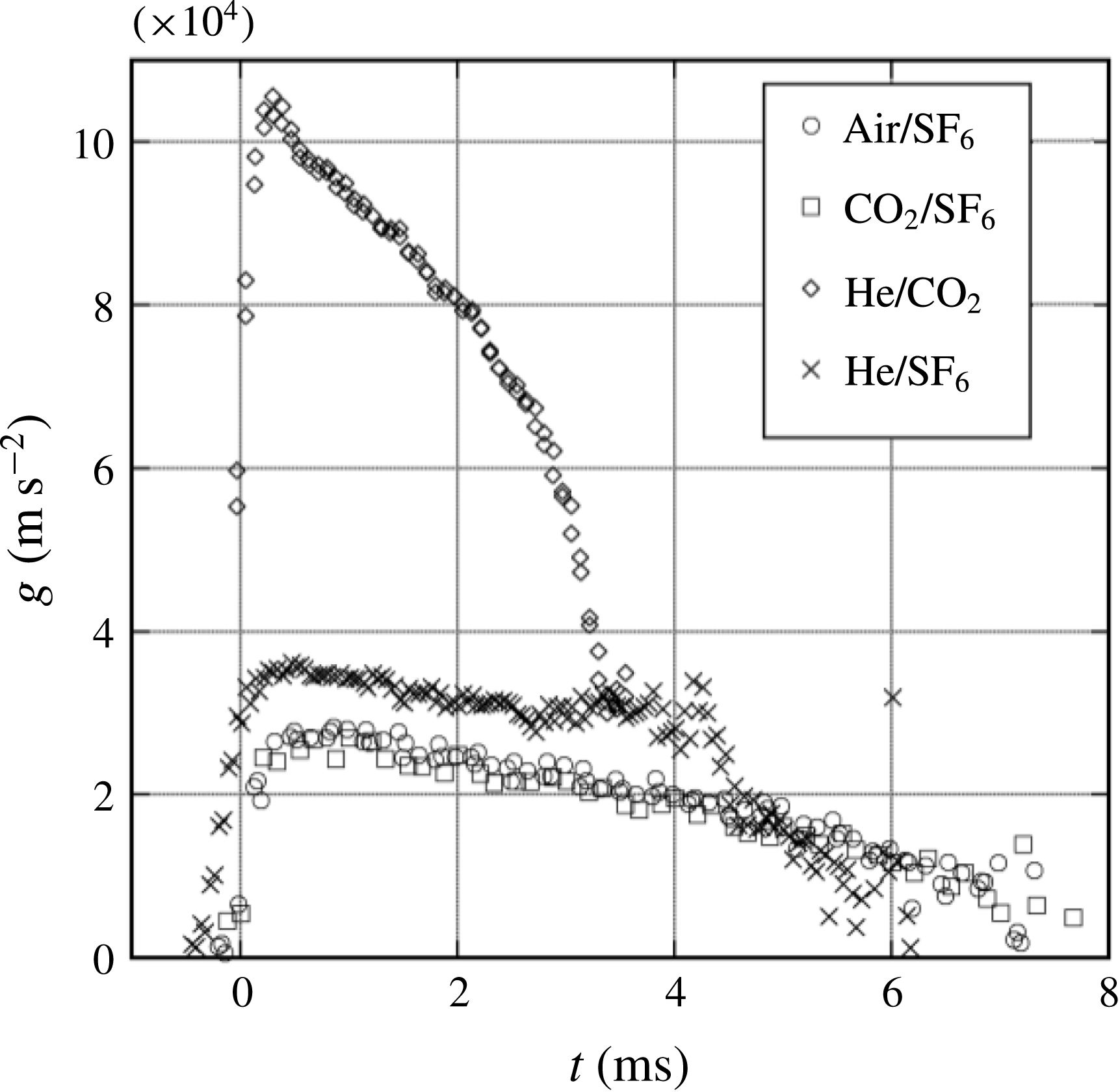
Acceleration profiles derived from flat interface displacement measurements for all of the gas combinations used. The helium combinations produce larger accelerations, while the
 $\text{air}\text{/}\text{SF}_{6}$
and
 $\text{CO}_{2}\text{/}\text{SF}_{6}$
combinations produce lower accelerations and have similar profiles.
 $\text{Air}\text{/}\text{SF}_{6}$
and
 $\text{CO}_{2}\text{/}\text{SF}_{6}$
plots are shown with only every fourth symbol displayed for clarity.
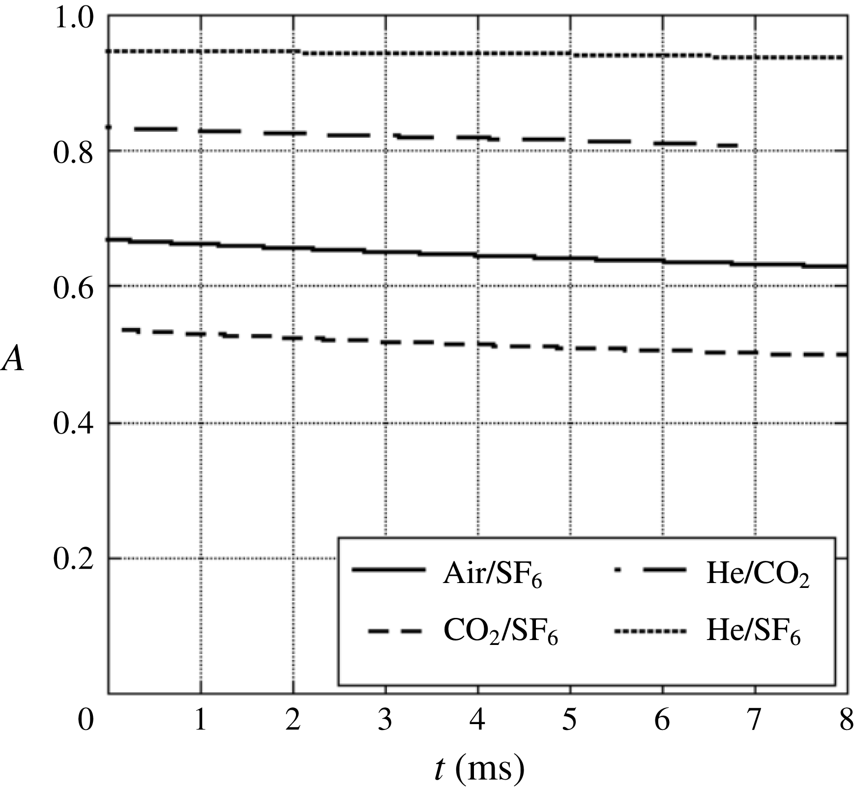
The Atwood number as a function of time for the gas pairs used herein. The Atwood number was derived from 1-D simulations for interfaces accelerated by a rarefaction wave.
A diagram of the ideal 1-D wave and interface interactions in the rarefaction tube in the
 $z$
–
 $t$
plane for
 $\text{CO}_{2}\text{/}\text{SF}_{6}$
. The fanned lines starting at
 $x=0$
represent the refracted rarefaction wave, while the initially vertical line represents the interface. The refraction of the rarefaction wave at the interface generates a reflected compression and causes the interface to accelerate toward the initial diaphragm location.

An image sequence from a 2-D
 $\text{CO}_{2}\text{/}\text{SF}_{6}$
3.5 wavelength experiment compared with concentration from a Miranda simulation at (a)
 $t=0$
ms, (b)
 $t=0.83$
ms, (c)
 $t=1.7$
ms, (d)
 $t=2.5$
ms, (e)
 $t=3.3$
ms, (f)
 $t=4.2$
ms, (g)
 $t=5.0$
ms, (h)
 $t=5.4$
ms, (i)
 $t=5.8$
ms, (j)
 $t=6.7$
ms, (k)
 $t=7.2$
ms. The evolution of the simulation and experiment are similar into the nonlinear phase. Secondary instability leads to the production of small scales in the experiment, while the simulation produces larger scale 2-D vortices and preserves the initial symmetry of the perturbations.

6 Qualitative observations
6.1 Two-dimensional results
Figure 6 shows the acceleration profiles resulting from the interaction of the rarefaction wave and the interface as illustrated in the characteristic diagram in figure 8 for each of the gas combinations used. The
 $\text{He}\text{/}\text{CO}_{2}$
combination produces the largest accelerations, while the
 $\text{CO}_{2}\text{/}\text{SF}_{6}$
combination produces the smallest acceleration. This interaction leads to a decrease in density with time, however, as shown in figure 7, this decrease results in little change in the Atwood number. Figure 9 shows a Mie scattering image sequence from a
 $\text{CO}_{2}\text{/}\text{SF}_{6}$
experiment initialized with a 2-D, 3.5 wavelength initial perturbation compared to the volume fraction of
 $\text{SF}_{6}$
from a 2-D Miranda simulation. Figure 9(a–c) shows the linear growth of the instability, characterized by the growth in amplitude of the sinusoid that describes the interface shape. Figure 9(d–f) shows the onset of nonlinearity during the roll up of the interface near the spike tips to form a row of line vortices, figure 9(g) shows the development of a secondary instability on the tips of the rolled up heavy gas region and figure 9(h–k) shows the turbulent breakdown of the interface and the mixing of the two gases in isolated locations near the centres of vorticity (experiment only). The pressure gradient at the interface continues to deposit vorticity, causing the gas that has rolled up to be pulled downward toward the interface. Secondary instabilities occur on the thin arms of the spike, where the interface thickness has become small due to straining, and generate smaller scales. The simulations in figure 9 show much of this character, but fail to produce turbulent mixing due to their 2-D nature and their tendency to preserve the symmetry of the initial perturbations.
An image sequence from a 2-D
 $\text{air}\text{/}\text{SF}_{6}$
2.5 wavelength experiment compared with a shadowgraph experiment and 2-D Laplacian of density (Settles Reference Settles2001) from a Miranda simulation at (a)
 $t=0.1$
ms, (b)
 $t=1.8$
ms, (c)
 $t=2.6$
ms and (d)
 $t=4.7$
ms. Here, experiments show little 3-D character at early times, exhibiting sharp single edges in the shadowgraph experiment, but become more 3-D at later times, showing multiple contours near the bubble tips.

Figure 10 shows a sequence of images from an
 $\text{air}\text{/}\text{SF}_{6}$
2.5 wavelength shadowgraph experiment compared with a Mie scattering experiment, along with the 2-D Laplacian of density from a Miranda simulation (Settles Reference Settles2001). The shadowgraph experiment shows that the perturbation is strongly two-dimensional at early times (outside what are assumed to be boundary effects), exhibiting a single visible interface. However, the bubbles appear to become three-dimensional at later times. The integrated structure of the turbulent mixing caused by the secondary instabilities can also be seen, and is noticeably absent in the 2-D simulation. Three-dimensionality is observed in these shadowgraph images by the presence of multiple light–dark contours around the interface location, whereas 2-D character is observed as a single sharp shadowgraph signal (a single light–dark band in the image).
An image sequence from a 2-D
 $\text{He}\text{/}\text{SF}_{6}$
1.5 wavelength experiment compared with concentration from a Miranda simulation at (a)
 $t=0$
ms, (b)
 $t=0.8$
ms, (c)
 $t=1.6$
ms, (d)
 $t=2.0$
ms, (e)
 $t=2.5$
ms, (f)
 $t=2.9$
ms, (g)
 $t=3.7$
ms, (h)
 $t=5.8$
ms. Large Atwood number experiments grow quickly, with a delayed roll up to a very large amplitude. The Mie scattering experiments exhibit less diffusion than simulations.

Figure 11 shows a comparison of volume fraction of
 $\text{SF}_{6}$
from a simulation with a
 $\text{He}\text{/}\text{SF}_{6}$
1.5 wavelength experiment. Differences in appearance are caused by smoke particles diffusing much more slowly than the gases, and hence do not represent the true concentration of heavy gas. At large Atwood number, the spike forms a narrow vertical structure with sharp gradients and a rounded tip. Note that this large Atwood number effect is also manifested slightly in the initial perturbation causing slightly narrower spike peaks, and wider bubble troughs. Thus the large Atwood number spike exhibits a delayed roll up relative to lower Atwood number experiments. At the latest times, the production of small scales is not reproduced well in the 2-D simulation.
6.2 Three-dimensional results
Schematic representations of imaged planes for 3-D experiments. The left half of the figure shows a bubble in the centre, while the right half shows a spike in the centre. Dashed lines are drawn in the contour plots to show how certain planes cut through the 3-D interface. These planar cuts lead to the interface profiles shown in the 2-D plots to the right of the contour plots. Panel (c) depicts the bubble/saddle plane, panel (d) depicts the spike/saddle plane, panel (e) depicts the bubble/extrema plane and panel (f) depicts the spike/extrema plane. For panels (e,f)
 $\tilde{x}=\sqrt{x^{2}+y^{2}}$
.

An image sequence comparing spike/extrema planes of
 $\text{air}\text{/}\text{SF}_{6}$
, 3-D 1.0 wavelength experiments to concentration from a Miranda simulation at (a)
 $t=0$
ms, (b)
 $t=1.2$
ms, (c)
 $t=2.5$
ms, (d)
 $t=3.7$
ms, (e)
 $t=4.3$
ms, (f)
 $t=5.0$
ms and (g)
 $t=6.2$
ms. The experiments are run with the spike in the centre using a diagonal laser sheet, and are compared with the periodic continuation of the diagonal plane of the simulations such that the spike appears in the centre. A vortex ring is seen to move upward from the interface. This ring eventually produces a secondary instability and mixing.

Figure 12 shows a schematic of laser sheet illumination planes used to visualize and extract features from the 3-D experiments. Four different types of experiments were conducted to visualize the instability in each of these planes. Experiments were conducted where either the bubble or spike is centred in the rarefaction tube, and the illumination plane cuts through the extrema of the interface (bubble/extrema, spike/extrema). Experiments were also conducted where the illumination plane cuts through the saddle points of the interface (bubble/saddle, spike/saddle). Figure 13 shows an
 $\text{air}\text{/}\text{SF}_{6}$
experiment visualized on the spike/extrema plane (figure 12
e) compared with an equivalent 3-D Miranda simulation. Excellent qualitative agreement is observed in the linear phase. However, as the nonlinear phase progresses, the experiments show a stronger breakdown of the bubble and spike structures due to wall interactions. The bubble/extrema and spike/extrema planes show the development of a single vortex ring structure associated with the 3-D RTI. However, perturbations of this form in low Atwood number experiments have been shown to generate two sets of vortex rings, one set travelling upward with the spikes and the other travelling downward with the bubbles (Wilkinson & Jacobs Reference Wilkinson and Jacobs2007). The lack of a secondary vortex ring observed here may be due to an interaction with the boundary layers on the test section walls, or may be a result of the larger Atwood numbers present in the experiments, which has been shown to decrease the strength of the secondary vortex ring in Rictmyer–Meshkov studies (Long et al.
Reference Long, Krivets, Greenough and Jacobs2009). Figure 14 shows the development of the spike in the spike/saddle plane (figure 12
b) compared with shadowgraph images, and the spike/extrema plane from a separate experiment. The spike tip is clearly visible in the shadowgraph images. In figure 14(b), the roll up of the spike generates smaller scales, whose 3-D character is visible as small ripples in the shadowgraph images. In figure 14(c), small scale turbulent structures can be seen in the shadowgraph images, while the diffusion that they generate is visible in the Mie scattering experiments. Additionally, since the shadowgraphs show an integrated view of the entire flow, both bubble/saddle and spike/saddle planes are visible. Near the top of the images, the spike/saddle plane is visible, and near the bottom, the bubble/saddle plane is visible, although distorted.
An image sequence comparing a 3-D
 $\text{air}\text{/}\text{SF}_{6}$
Mie scattering experiments (spike/saddle left, spike/extrema right) and an
 $\text{air}\text{/}\text{SF}_{6}$
shadowgraph experiment (centre) at (a)
 $t=2.6$
ms, (b)
 $t=4.6$
ms and (c)
 $t=6.8$
ms. The shadowgraph images show the clear development of the spike/saddle plane, and a view of the distorted bubble/saddle plane on the wall. Three-dimensional secondary instability can be seen emerging in panel (b).

An image sequence comparing bubble/extrema planes of 3-D
 $\text{air}\text{/}\text{SF}_{6}$
1.0 wavelength experiments to concentration from a Miranda simulation at (a)
 $t=0$
ms, (b)
 $t=1.2$
ms, (c)
 $t=2.5$
ms, (d)
 $t=3.7$
ms, (e)
 $t=4.3$
ms, (f)
 $t=5.0$
ms and (g)
 $t=6.2$
ms. The experiments are run with the bubble in the centre, and are compared with the diagonal plane of the simulations. The experiments exhibit a pronounced secondary instability at the bubble tips, while strong mixing can be observed in the bubble vortex ring in the simulations.

An image sequence comparing a 3-D
 $\text{air}\text{/}\text{SF}_{6}$
Mie scattering experiment (bubble/saddle left, bubble/extrema right) and an
 $\text{air}\text{/}\text{SF}_{6}$
shadowgraph experiment (centre) at (a)
 $t=1.5$
ms, (b)
 $t=2.7$
ms, (c)
 $t=4.5$
ms and (d)
 $t=6.2$
ms. The shadowgraph images bear a strong resemblance to the bubble/spike plane images. Panel (c) shows the emergence of a secondary Rayleigh–Taylor instability which envelopes the entire bubble by panel (d).

Figure 15 shows a similar set of images to figure 13, but for a bubble experiment in the bubble extrema plane (d in figure 12). Excellent agreement with the simulation is observed through the linear stage, and the shape of the bubble in the nonlinear regime is similar to that produced by simulations. In the last panel, a pronounced secondary RTI at the bubble tip is observed, and the spikes are strongly affected by the walls. Figure 16 shows the bubble/saddle plane (figure 12
c) compared with shadowgraph images of the bubble, and the bubble/extrema plane from a separate experiment. These images show evidence of vortex ring development in the second panel, and also display the 3-D nature of the secondary instability at the bubble tip. Finally, the last panel shows the secondary instability engulfing the entire bubble. Figure 17 shows a 3-D visualization from a numerical simulation using
 $\text{air}\text{/}\text{SF}_{6}$
. This visualization shows the basic shapes of the bubbles and spikes from a numerical simulation, and the development of the 3-D vortex ring structure. By figure 17(d) the bubble takes on a very axisymmetric shape, while in figure 17(e) a secondary instability is observed. Finally, in figure 17(f), smaller scale turbulent structures begin to appear.
Experimental images of the spikes show good qualitative agreement with simulations, but exhibit a greater degree of secondary Kelvin–Helmholtz instability near the spike tips. The secondary instability in the spike/saddle plane is the only secondary instability observed in the 3-D simulations. This more pronounced occurrence of instability in experiments may be due to a lack of small scale perturbations required to seed the secondary instability in the simulations, or the emergence of the secondary instability in experiments from scales unresolved in the simulations. Additionally, the numerical scheme used to compute the simulations requires a minimum interface thickness, forcing the Miranda code to increase the width of the interface, which may stabilize the secondary instability.
Bubbles in experiments exhibit a very strong secondary RTI that is not observed in the simulations. This secondary instability can be seen emerging in figure 16(c), and is produced by a large effective acceleration,
 $$\begin{eqnarray}g_{b}=g+\ddot{a}_{b},\end{eqnarray}$$
experienced at the bubble tip in combination with the thinning of the interface caused by straining due to the growth of the bubble. This secondary RTI leads to the rapid production of smaller scales, and quickly engulfs the entire bubble. The absence of this secondary instability in simulations may again be due to the increased grid dependent diffusivity in the simulation, or to the lack of small scale seed perturbations.
Isosurfaces of 40–60 % concentration in a 3-D
 $\text{air}\text{/}\text{SF}_{6}$
Miranda simulation showing the shape of the single-mode 3-D RTI at (a)
 $t=0$
ms, (b)
 $t=2.3$
ms, (c)
 $t=4.1$
ms, (d)
 $t=4.8$
ms, (e)
 $t=5.8$
ms and (f)
 $t=6.8$
ms. By panel (d) the bubbles take on a very axisymmetric shape.

7 Late-time velocity behaviour
7.1 Two-dimensional results
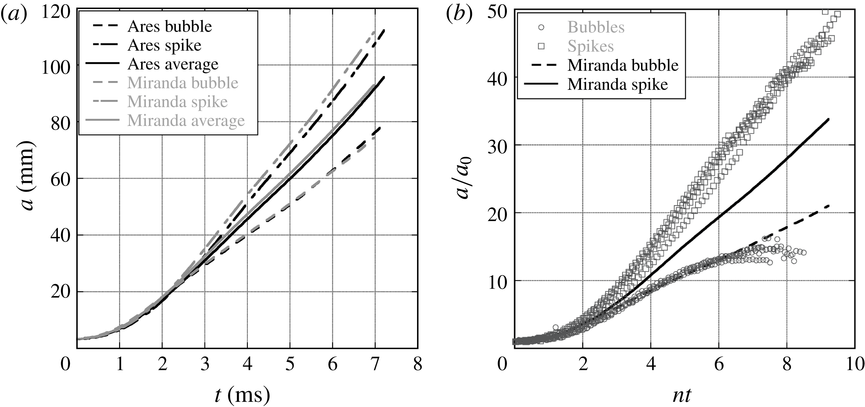
Amplitudes were extracted from experiments and simulations, and subsequently Froude numbers were calculated to compare with single-mode nonlinear analyses. Bubble and spike amplitudes were extracted using the methods described in § 5. Figure 18 shows a comparison of amplitude trends from Ares and Miranda 2-D
 $\text{air}\text{/}\text{SF}_{6}$
1.5 wavelength simulations. Good agreement is observed between the codes for this case and for the 2-D
 $\text{air}\text{/}\text{SF}_{6}$
2.5 wavelength case (
 $\text{air}\text{/}\text{SF}_{6}$
was the only gas combination used in Ares). Figure 18 also shows a comparison of experimental bubble and spike amplitudes to a Miranda simulation. Good agreement for bubble amplitudes is observed at early times. However, the experimental spike amplitudes are significantly larger than given by the simulation. This amplitude plot clearly shows the early time linear region, characterized by exponential growth, followed by the nonlinear region which is characterized by saturation to a nearly constant velocity at late times.
A comparison of amplitudes from 2-D numerical simulations for
 $\text{air}\text{/}\text{SF}_{6}$
, 1.5 wavelengths (a), and non-dimensional amplitudes for
 $\text{air}\text{/}\text{SF}_{6}$
1.5 wavelength experiments compared to a Miranda simulation (b). The amplitude trends for Ares and Miranda are very similar. The amplitude trends show the early time exponential growth which saturates to nearly constant growth in the nonlinear region. Note that here
 $n$
is the growth rate for linear growth that takes the form
 $a=a_{0}\cosh (nt)$
.
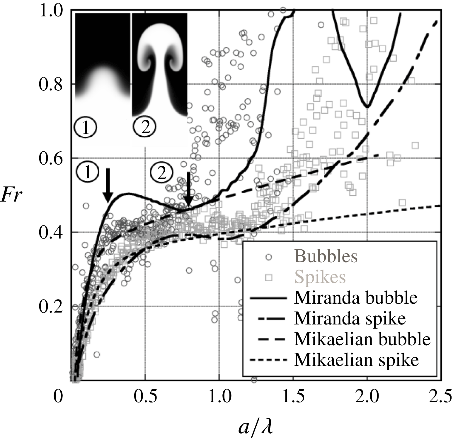
Typical late-time velocity behaviour for 2-D low Atwood number, large wavenumber experiments from
 $\text{CO}_{2}\text{/}\text{SF}_{6}$
(
 $A=0.49$
), 3.5 wavelength experiments. Intermediate-time constant velocity behaviour is observed, but at a larger Froude number than predicted by the Goncharov model. The model of Mikaelian (Reference Mikaelian2009) seems to predict spike Froude numbers well. Two images are superposed on the graph corresponding to
 $a_{b}/\unicode[STIX]{x1D706}=0.25$
(left, less developed) and
 $a_{b}/\unicode[STIX]{x1D706}=0.76$
(right, more roll up).
Typical late-time velocity behaviour for 2-D low Atwood number, large wavenumber experiments from
 $\text{air}\text{/}\text{SF}_{6}$
(
 $A=0.63$
), 2.5 wavelength experiments. Intermediate-time constant velocity behaviour is again observed at a larger Froude number than predicted by the Goncharov model. The model of Mikaelian (Reference Mikaelian2009) seems to predict spike Froude numbers well. Two images are superposed on the graph corresponding to
 $a_{b}/\unicode[STIX]{x1D706}=0.25$
(left, less developed) and
 $a_{b}/\unicode[STIX]{x1D706}=0.76$
(right, more roll up).
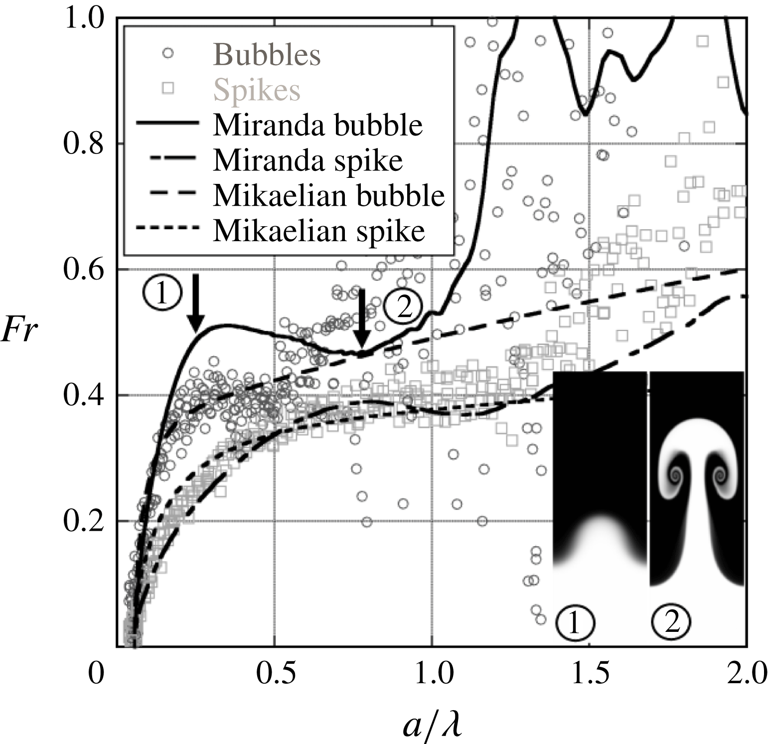
The Froude number is a convenient parameter that shows the non-dimensional velocity of the interface, and in addition, can be thought of as relating the strength of inertial forces to buoyancy forces. The balance of these two forces shows the nonlinear transition of the instability where buoyancy forces are offset by drag, causing a decrease in the bubble and spike acceleration. Figures 19 and 20 are plots of the Froude numbers calculated using (1.3) for four 3.5 wavelength,
 $\text{CO}_{2}\text{/}\text{SF}_{6}$
experiments, and four
 $\text{air}\text{/}\text{SF}_{6}$
experiments, respectively. The scatter in these plots is caused by the numerical derivatives used to calculate
 $V_{b/s}$
and
 $g$
in (1.3). Additionally, since the data are produced from images, pixel aliasing can exacerbate this scatter. The plots show that after an initial growth stage the dimensionless velocity reaches a nearly constant value for bubbles and spikes at intermediate times, and then increases at the latest times. This reacceleration is similar to the effect shown by Ramaprabhu et al. (Reference Ramaprabhu, Dimonte, Woodward, Fryer, Rockefeller, Muthuraman, Lin and Jayaraj2012) for 3-D and Reckinger et al. (Reference Reckinger, Livescu and Vasilyev2010) for 2-D bubbles. Ramaprabhu et al. (Reference Ramaprabhu, Dimonte, Woodward, Fryer, Rockefeller, Muthuraman, Lin and Jayaraj2012) propose that the secondary KH vortex doublet or ring induces an additional velocity on the bubble (vortex pairing effect), providing the driving force for reacceleration. Images from 2-D Miranda simulations are superposed on figures 19 and 20, and correspond to
 $a_{b}/\unicode[STIX]{x1D706}=0.25$
and
 $a_{b}/\unicode[STIX]{x1D706}=0.76$
. Although it is difficult to pinpoint the exact value of
 $a/\unicode[STIX]{x1D706}$
that reacceleration is observed for these experiments,
 $a_{b}/\unicode[STIX]{x1D706}=0.25$
, and
 $a_{b}/\unicode[STIX]{x1D706}=0.76$
are approximately when the bubble Froude number saturates, and then reaccelerates, respectively. In 2-D simulations, these points represent the first local maximum of the Froude number, and then the subsequent local minimum. The images show that
 $a_{b}/\unicode[STIX]{x1D706}=0.25$
appears to correspond to an experimental time just prior to the onset of roll up while
 $a_{b}/\unicode[STIX]{x1D706}=0.76$
corresponds to a point well past where roll up first occurs. It should be noted that the bubble Froude number prior to reacceleration is larger in the present experiments than the value of
 $1/\sqrt{3\unicode[STIX]{x03C0}}$
(
 ${\approx}0.33$
) found in the experiments of Wilkinson & Jacobs (Reference Wilkinson and Jacobs2007) and predicted by Goncharov (Reference Goncharov2002). This disagreement is likely due to the effects of variable acceleration and compressibility, which the model neglects and which were not present in Wilkinson’s experiments. We expect the effects of variable acceleration to be partially accounted for by using the time varying acceleration in the definition of Froude number. Additionally, the model of Goncharov (Reference Goncharov2002) does not produce reacceleration, and fails to predict the late-time behaviour. Ramaprabhu et al. (Reference Ramaprabhu, Dimonte, Woodward, Fryer, Rockefeller, Muthuraman, Lin and Jayaraj2012) point out that this reacceleration represents a departure from potential flow models like that of Goncharov (Reference Goncharov2002). Figures 19 and 20 also show the results from the Mikaelian model (Mikaelian Reference Mikaelian2009) which accounts for variable acceleration and variable density. To produce curves for the Mikaelian model, (1.5) through (1.7) are solved numerically with
 $k$
,
 $\unicode[STIX]{x1D702}_{0}$
,
 $\dot{\unicode[STIX]{x1D702}}_{0}=0$
and the function of acceleration with time as input parameters. The interface acceleration is input as a curve fit to the experimental acceleration profile. This curve fit acceleration profile is then used to determine the densities of the light and heavy gases using isentropic rarefaction wave theory similar to equations (3.1) through (3.4).
For the smaller Atwood number, and larger wavenumber experiments, the late-time velocity Froude number is better predicted by the model of Mikaelian (Reference Mikaelian2009) than by the model of Goncharov (Reference Goncharov2002). Good agreement is observed between the larger wavenumber experiments, simulations, and models for the spike, until the Froude number begins to increase again at late times. The late-time increase in Froude number, similar to that observed by Wilkinson & Jacobs (Reference Wilkinson and Jacobs2007), is observed in the simulations at a larger value of
 $a/\unicode[STIX]{x1D706}$
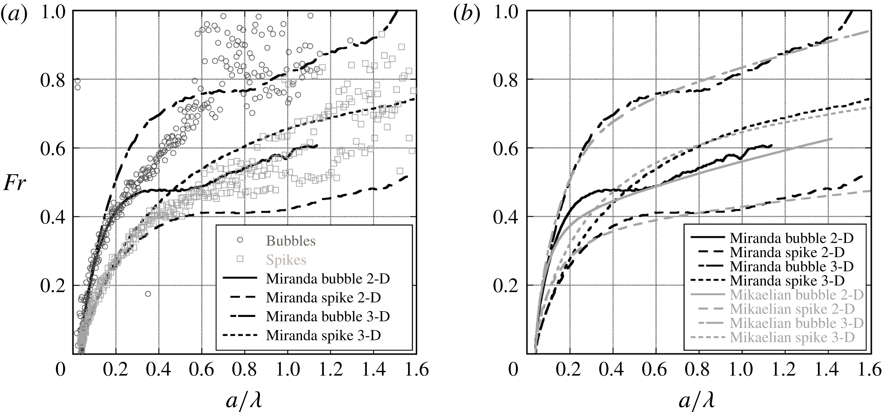
than in experiments. The 2-D bubble simulation captures the character of the bubble Froude number, but overshoots the region of constant Froude number and then decreases to meet it, while the Mikaelian model captures the transition better than the simulation. Some of this discrepancy can be attributed to the different mechanisms described by Wei & Livescu (Reference Wei and Livescu2012) and Ramaprabhu et al. (Reference Ramaprabhu, Dimonte, Woodward, Fryer, Rockefeller, Muthuraman, Lin and Jayaraj2012). The experiments tend to have their symmetry broken, and hence progress as described by Ramaprabhu et al. (Reference Ramaprabhu, Dimonte, Woodward, Fryer, Rockefeller, Muthuraman, Lin and Jayaraj2012), while the 2-D simulations tend to preserve symmetry and progress as described by Wei & Livescu (Reference Wei and Livescu2012). However, these simulations were not run far enough in time to compare with the late-time ‘chaotic development’ of Wei & Livescu (Reference Wei and Livescu2012). For the lower wavenumber experiments, the Froude number appears to be bounded by the 2-D and 3-D simulations, possibly indicating a 3-D effect is present.
Figure 21 shows a comparison of Froude numbers for simulations and models with those from experiments having 1.5 wavelengths. For this wavenumber, experiments have the largest departures from constant Froude number behaviour for the same Atwood numbers. These low wavenumber experiments never approach a constant Froude number, exhibiting Froude numbers that grow continuously. The difference between Froude numbers in small and large wavenumber experiments is possibly due to slower linear RTI growth (proportional to
 $\sqrt{k}$
) for the 1.5 wavelength experiment leading to a nonlinear phase that is not observed during the timeframe of the experiment. Additionally, the bubbles and spikes for the two wavenumbers will see different time histories of density due to their different initial amplitudes and growth rates. Another possible cause of the different Froude number behaviour for small wavenumbers, is that a 3-D distortion of the interface in the
 $y$
direction leads to a large wavelength, out-of-plane mode, that is still growing linearly. The Mikaelian model and the simulations agree well with each other, with the biggest disagreement occurring in the transition region for 2-D bubbles.
The development of the Froude number for 2-D
 $\text{CO}_{2}\text{/}\text{SF}_{6}$
(
 $A=0.49$
), 1.5 wavelength experiments (a), and a comparison of simulations and the model of Mikaelian (Reference Mikaelian2009) (b). Experiments differ from 2-D simulations at late times, with Froude numbers that more resemble 3-D growth. The model of Mikaelian (Reference Mikaelian2009) compares well with 2-D and 3-D simulations.
7.2 Three-dimensional results
Figure 22 shows the position of the spike, bubble, flat interface and saddle points as the RTI develops and travels down the test section. Good agreement is observed between experiments and simulations for the flat interface and spike locations. Slight disagreement is observed for the saddle point, likely due to the distortion of the saddle points in experiments by boundary layer effects. However, agreement between the saddle points in experiments and simulations is good at early times further justifying the spike and bubble separation technique described in § 5, above.
Trajectories for various points on the interface from 3-D,
 $\text{air}\text{/}\text{SF}_{6}$
(
 $A=0.63$
) experiments. The spike, saddle and flat interface position are shown compared with a numerical simulation (a), as well as the bubble, saddle and flat interface positions (b). This simulation produces spike positions that agree well with data, however, the bubble positions develop large discrepancies.
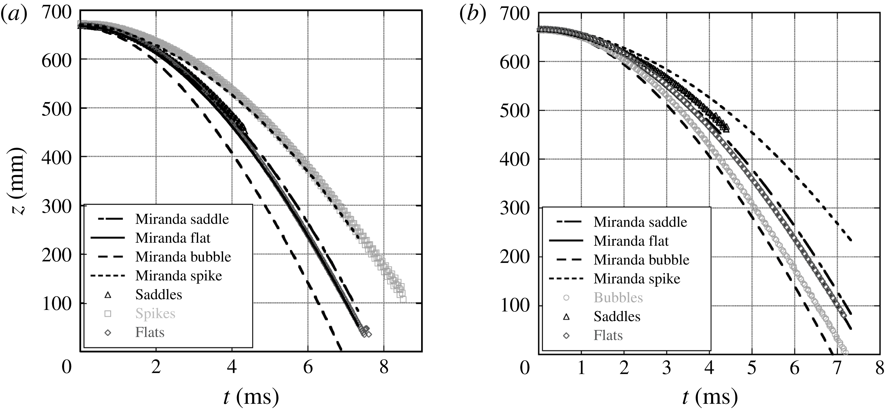
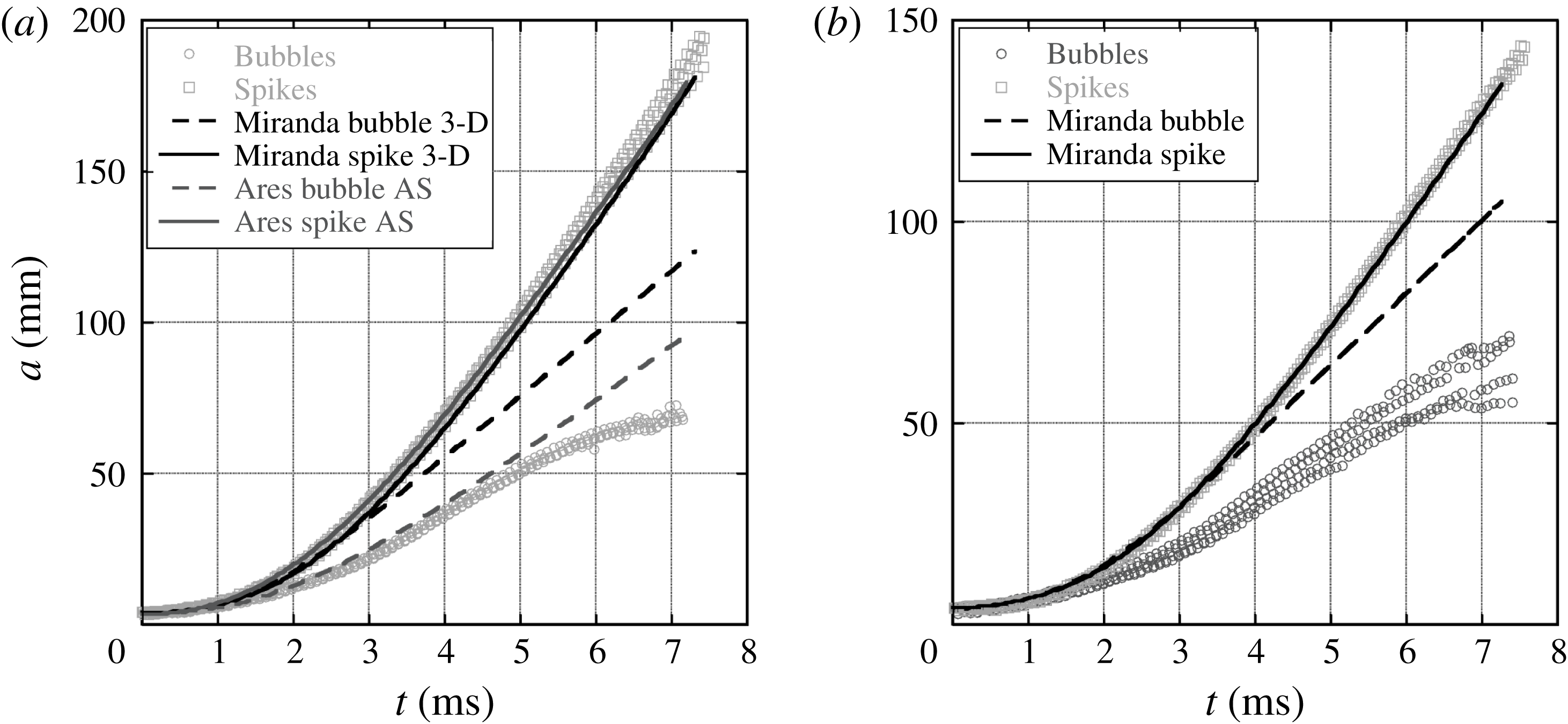
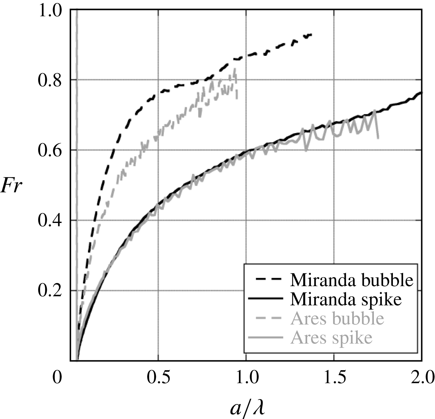
Figure 23 shows the amplitude of the bubbles and spikes in the 3-D RTI simulations and experiments as they develop with time. Similar to what is observed in the 2-D results, good agreement between simulation and experiments is observed for spikes, while the bubble amplitudes fall well below the simulations. The simulations exhibit similar early time growth for bubbles and spikes, whereas the bubble and spike behaviours depart soon after the start of the experiment. Also shown in this figure is an Ares axisymmetric bubble simulation that shows much better agreement with the bubble measurements at early times, but does not exhibit a decaying growth rate at late times as is observed in the experiments. The boundary layers developing in the experiments may cause the bubbles to grow more axisymmetrically, thus yielding better agreement with the axisymmetric simulation. Figure 24 shows the Froude number trends for the axisymmetric Ares simulation compared to the Cartesian 3-D Miranda simulation. Froude number trends for spikes for both simulations are nearly identical. However, the axisymmetric bubble begins to saturate much earlier than the Cartesian 3-D bubble.
Amplitudes from 3-D, single-mode experiments with
 $\text{air}\text{/}\text{SF}_{6}$
(a,
 $A=0.63$
) and
 $\text{CO}_{2}\text{/}\text{SF}_{6}$
(b,
 $A=0.49$
). Good agreement is observed between simulations and experiments for spike amplitudes for both gas pairs. The bubble amplitudes disagree greatly with 3-D Miranda simulations, however, agreement with an axisymmetric Ares simulation is much better.
Spike and bubble Froude numbers from an axisymmetric Ares simulation and a 3-D Miranda simulation. Good agreement is observed for spikes and not for bubbles.
Froude numbers for 3-D,
 $\text{air}\text{/}\text{SF}_{6}$
(a,
 $A=0.63$
), and
 $\text{CO}_{2}\text{/}\text{SF}_{6}$
(b,
 $A=0.49$
) experiments compared with simulations and theory. Good agreement is seen for spikes at early times, while the bubbles reach late-time constant velocity much more quickly than simulations, and appear to approach the asymptotic Froude number found by Goncharov (Reference Goncharov2002). Good agreement between the simulations and the theory of Mikaelian (Reference Mikaelian2009) is observed.
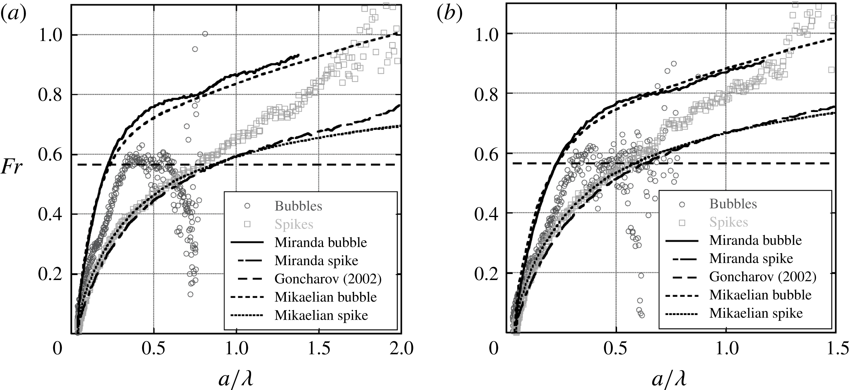
Figure 25 shows the late-time velocity behaviour of the 3-D RTI. The spike Froude number in the Miranda simulation agrees well with the experiments for both Atwood numbers, but diverges at late times, while the bubbles are seen to grow more slowly in experiments. The simulation bubble Froude number agrees only briefly with the experiments, with the experiments saturating very quickly, and appearing to reach the asymptotic Froude number,
 $Fr=1/\sqrt{\unicode[STIX]{x03C0}}$
(
 $Fr\approx 0.56$
), given by the incompressible theory of Goncharov (Reference Goncharov2002). This reduced Froude number may be explained by the existence of boundary layers in the experiments. Davies & Taylor (Reference Davies and Taylor1950) showed that, for bubbles rising at constant velocity in a cylindrical tube of radius
 $a_{tube}$
, the bubble velocity
 $V_{b}$
for small thicknesses
 $t_{h}$
of heavy fluid between the bubble and the wall,
 $t_{h}/a_{tube}\ll 1$
, is approximately
 $$\begin{eqnarray}V_{b}\approx \frac{2\sqrt{2g}}{a_{tube}}(t_{h}\sqrt{z_{b}}),\end{eqnarray}$$
where
 $z_{b}$
is the extent of the bubble, and the combination
 $t_{h}\sqrt{z_{b}}$
is approximately constant. Strain due to the motion of the walls in the bubble reference plane thins the layer of heavy fluid near the wall relative to the rising bubble case, and reduces the effective thickness
 $t_{h}$
in experiments. Since
 $t_{h}$
is reduced, the bubble velocity could be decreased relative to the simulations, which, since they have periodic boundary conditions, produce no wall boundary layers. At the latest times, the bubble Froude numbers are seen to decrease, indicating that the bubble has exited the rarefaction wave and is thus decelerated relative to the flat interface (as the bubbles typically travel far ahead of the flat interface), and these data should not be used for comparison.
Froude number trends for 2-D, large
 $A$
,
 $\text{He}\text{/}\text{SF}_{6}$
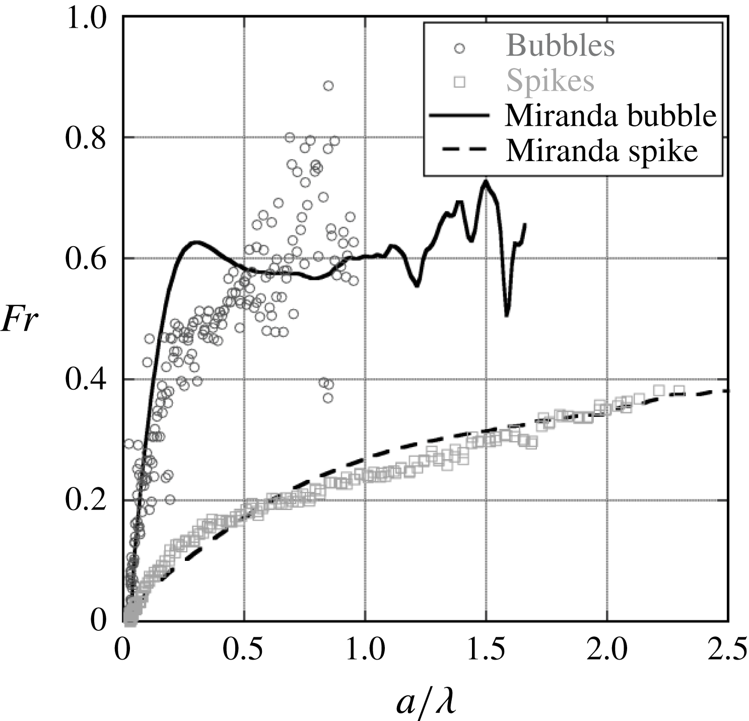
experiments. Neither the bubbles nor the spikes appear to be approaching a constant value of Froude number. This behaviour is in contrast to low
 $A$
experiments with larger wavenumbers, which appears to indicate free-fall behaviour.
8 Two-dimensional free-fall behaviour
At the largest Atwood numbers,
 $A=0.82$
and
 $A=0.94$
in the 2-D experiments, the spikes are not observed to reach constant velocity (or Froude number). Figure 26 shows the Froude number for large
 $A$
,
 $\text{He}\text{/}\text{SF}_{6}$
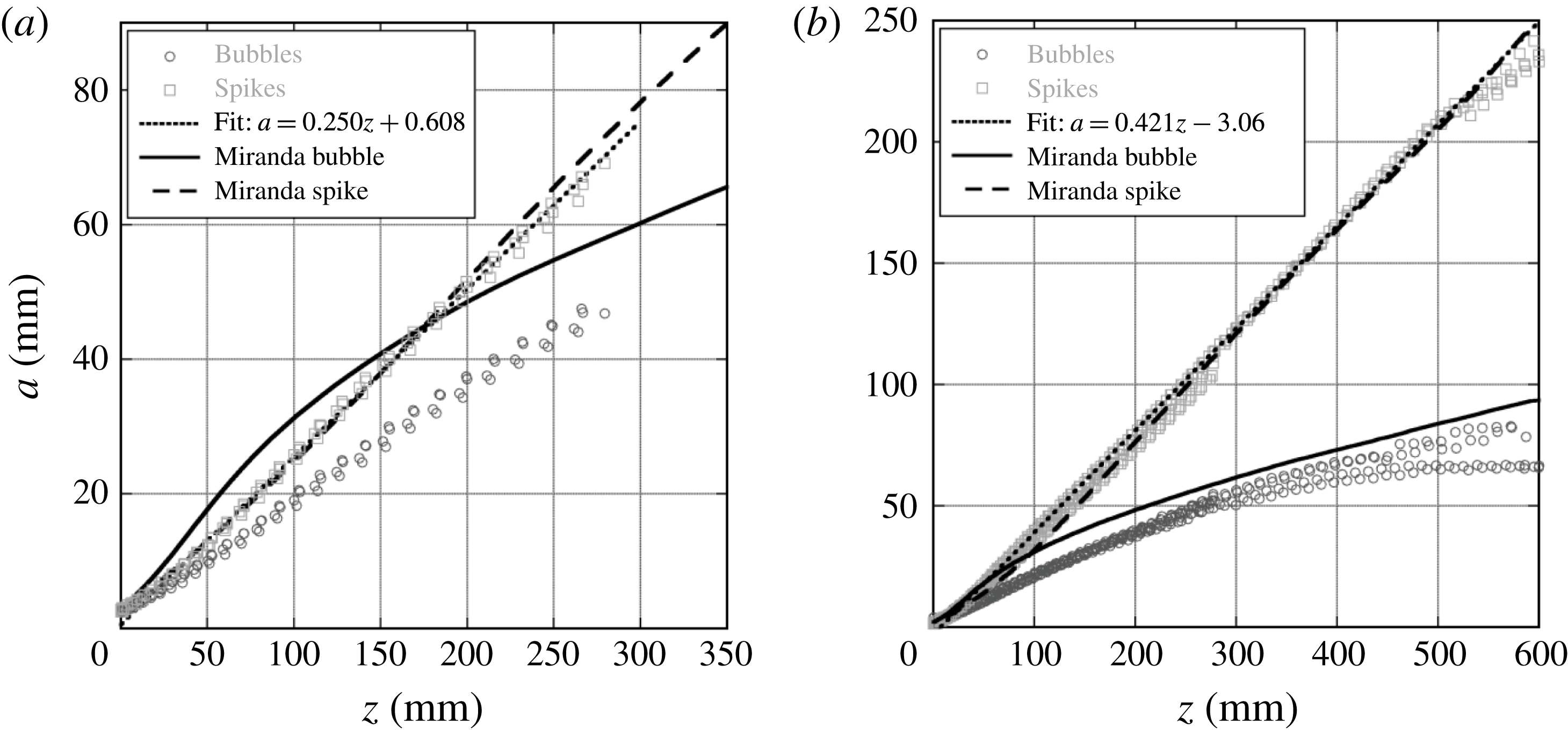
2-D experiments, where bubble and spike Froude numbers do not appear to approach constant values. Figure 27 shows the amplitude of the RTI with respect to the displacement of the flat interface. These plots show the amplitude of the spikes increasing proportional to the flat interface displacement, following
 $a=a_{0}+\unicode[STIX]{x1D712}z$
, where
 $\unicode[STIX]{x1D712}$
can be defined as the free-fall growth coefficient, indicating free-fall-like behaviour. For true free-fall behaviour,
 $\unicode[STIX]{x1D712}=1$
. However, here the constant is less than one and appears to decrease with decreasing Atwood number. This formulation for free-fall amplitude is proposed to account for the variable acceleration of the interface, similar to the formulation of Zaytsev et al. (Reference Zaytsev, Krivets, Mazilin, Titov, Chebotareva, Nikishin, Tishkin, Bouquet and Haas2003) for mixing layer growth. The bubble amplitudes in the experiments also appear to be proportional to the displacement of the interface. Free-fall behaviour is expected in the limit
 $A\rightarrow 1$
when the drag on the spike goes to zero. This limit would only be seen when the spike is penetrating into vacuum, and is detached from the interface. For
 $A<1$
, there will always be some drag which should eventually lead to a terminal velocity. However, this velocity may take increasingly longer times to reach as
 $A\rightarrow 1$
. The numerical simulations capture the spike behaviour very well, exhibiting some curvature in the plot that is not observed in experiments at early times. The bubble amplitude in the simulations shows large departures from the experimental data, which is more pronounced for the
 $A=0.82$
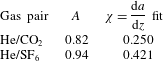
experiments. This may be due to the influence of the boundary layers in the experiments, or the preservation of symmetry in the simulations which is quickly broken in the experiments. Table 3 shows extracted free-fall growth coefficients and Atwood numbers for experiments exhibiting free-fall-like behaviour. These coefficients are much lower than the predicted value of
 $\unicode[STIX]{x1D712}=1$
for
 $A\rightarrow 1$
(Mikaelian Reference Mikaelian2008), and
 $\unicode[STIX]{x1D712}=A$
predicted by Baker et al. (Reference Baker, Meiron and Orszag1980). This behaviour is similar to that observed by Youngs (Reference Youngs1984), who found that the spike penetration for large Atwood number fell well short of free fall for large density ratios (
 $A\rightarrow 1$
). Free-fall behaviour was not observed in the 3-D experiments due mainly to their lower Atwood numbers.
RTI amplitude for high Atwood number experiments conducted with
 $\text{He}\text{/}\text{CO}_{2}$
(a,
 $A=0.82$
), and
 $\text{He}\text{/}\text{SF}_{6}$
(b,
 $A=0.94$
). Typical late-time constant velocity behaviour is not observed, however, the straight line curve fits indicate free-fall behaviour, with a reduced constant of proportionality.
Free-fall growth coefficients for high Atwood number, single-mode experiments.
9 Reynolds number
The Reynolds number plays an important role in characterizing the transition to turbulence for all flows, including RTI. For example, when a critical Reynolds number is reached in the shear layer, large structures present at lower Reynolds numbers remain. However, there is a significant increase in smaller scale turbulence resulting in the enhancement of molecular mixing (Dimotakis Reference Dimotakis2000). This transition has been termed the mixing transition. For most experiments conducted herein, the interface maintains some of its original large scale coherence, with a small amount of small scale mixing induced by secondary instability. However, the degree of turbulent mixing present is significantly less than that observed in other flows (such as the shear layer) that have undergone the mixing transition. Cook & Dimotakis (Reference Cook and Dimotakis2001) have proposed the mixing transition to occur in self-similar RTI when the Reynolds number computed using
 $Re=a{\dot{a}}/\bar{\unicode[STIX]{x1D708}}$
exceeds a value of 1000–2000, where
 $\bar{\unicode[STIX]{x1D708}}=(\unicode[STIX]{x1D707}_{1}+\unicode[STIX]{x1D707}_{2})/(\unicode[STIX]{x1D70C}_{1}+\unicode[STIX]{x1D70C}_{2})$
with
 $\unicode[STIX]{x1D707}_{2}$
and
 $\unicode[STIX]{x1D707}_{1}$
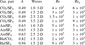
the dynamic viscosities of the light and heavy fluid, respectively. Table 4 shows the peak value of the Reynolds number achieved at the end of single-mode experiments which show values of the Reynolds number an order of magnitude larger than that predicted by Cook & Dimotakis (Reference Cook and Dimotakis2001) to define the mixing transition. Thus, even though our experimental values far exceed the predicted transition point, the mixing transition does not appear have been achieved, and turbulent RTI development is only beginning to be observed at the end of experiments. This transition criterion, however, uses a Reynolds number definition appropriate for a self-similar flow, and may not be appropriate for the behaviour of isolated modes. Self-similar theory generally assumes broadband perturbations which can interact more readily through nonlinear mechanisms (Cabot Reference Cabot2006). Thus an alternative definition may be necessary for this flow.
Peak Reynolds numbers developed in 2-D single-mode experiments, and perturbation Reynolds numbers. In these experiments larger Atwood numbers and smaller wavenumbers tend to produce the largest Reynolds numbers. Perturbation Reynolds numbers are sufficiently high to reach late stage development.
Wei & Livescu (Reference Wei and Livescu2012) considered a different type of transition defined when a critical value of the perturbation Reynolds number is exceeded. Their perturbation Reynolds number was proposed to indicate the growth stages the instability would transition through. They found that when the Reynolds number defined by
 $$\begin{eqnarray}Re_{p}=\frac{\unicode[STIX]{x1D706}}{\bar{\unicode[STIX]{x1D708}}}\sqrt{\frac{Ag\unicode[STIX]{x1D706}}{1+A}},\end{eqnarray}$$
exceeds a value of
 $1\times 10^{4}$
, that chaotic development occurs, characterized by phases of random acceleration and deceleration. Table 4 also contains the perturbation Reynolds number of Wei & Livescu (Reference Wei and Livescu2012), that shows that all of the
 $Re_{p}$
values are greater than the value of
 $1\times 10^{4}$
described by Wei and Livescu as the minimum required for ‘chaotic development’. However, it is difficult to compare with the results of Wei and Livescu since the experiments tend to break symmetry. On the other hand, the simulations do show some evidence of the chaotic-like reacceleration behaviour present in the chaotic development regime of Wei and Livescu. However, due to the subgrid model, the simulations have additional viscosity at late times, and the simulations have insufficient durations to clearly show the stationary bubble front acceleration of Wei and Livescu. Differences between the 2-D simulations and experiments may be due to the fact that the simulations have become chaotic, resulting in small differences in initial conditions leading to large differences in late-time development. However, it is difficult to determine if something similar has occurred in experiments due to their early symmetry breaking, and the presence of boundary layers. The experiments exhibit good macro-scale repeatability, however they all have slight underlying differences due to thermal fluctuations and timing jitter in the initialization of the experiment. Figure 28 shows the growth of the Reynolds number with time. Similar power law growth is observed at intermediate times for both Atwood numbers, and appears to be proportional to
 $t^{3}$
, implying a
 $t^{2}$
growth in amplitude that is similar to self-similar growth. However, it should also be noted that Wei and Livescu found chaotic development to produce
 $t^{2}$
growth in the mean. Therefore, the experimental finding compares favourably with this result. The Reynolds number for the lower Atwood number appears to decrease in power from
 $t^{3}$
at the latest times, indicating a transition to increased dissipation.
The Reynolds number,
 $Re=a{\dot{a}}/\bar{\unicode[STIX]{x1D708}}$
, for
 $\text{He}\text{/}\text{SF}_{6}$
1.5 wavelength and
 $\text{CO}_{2}\text{/}\text{SF}_{6}$
3.5 wavelength experiments.

10 Conclusions
The Rayleigh–Taylor instability has been studied in gas phase experiments and simulations with large accelerations. These accelerations are generated by using a rarefaction wave that accelerates a stably stratified two-fluid system separated by a diffuse interface, making it Rayleigh–Taylor unstable. Using gases allows the study of the RTI at Atwood numbers up to
 $A=0.94$
for
 $\text{He}\text{/}\text{SF}_{6}$
, and using the interface perturbation techniques of Jacobs et al. (Jones & Jacobs Reference Jones and Jacobs1997; Collins & Jacobs Reference Collins and Jacobs2002; Jacobs et al.
Reference Jacobs, Krivets, Tsiklashvili and Likhachev2013) 2-D and 3-D single-mode perturbations are generated. However, the use of the rarefaction wave leads to non-constant acceleration and a non-uniform density distribution. Additionally, gases allow the study of the instability originating from a diffuse interface using a miscible combination. Hence, these represent the first gas phase single-mode RTI experiments, and the only single-mode RTI experiments that are carried out to very late non-dimensional time and high Reynolds number. The experiments resulting from this range of perturbations allow the study of 2-D and 3-D single-mode RTI into the nonlinear regime, while the simulations allow the study of the instability with idealized initial and boundary conditions.
RTI evolution is recorded using shadowgraphy on pure gases or planar laser Mie scattering of smoke particles seeded in the heavy gas, and by recording images using up to three high-speed CMOS cameras. The moderate Atwood number
 $\text{CO}_{2}\text{/}\text{SF}_{6}$
and
 $\text{air}\text{/}\text{SF}_{6}$
combinations show constant velocity plateaus where the Froude numbers approach a constant value at intermediate times for 2.5 and 3.5 wavelength experiments, but with values larger than those predicted by Goncharov (Reference Goncharov2002). Using the model of Mikaelian (Reference Mikaelian2009) produces improved agreement in the intermediate-time plateau velocity Froude number by accounting for some compressibility effects including variable acceleration and density. This model, however, fails to predict the reacceleration phenomenon in experiments which may be caused by the production of vortex doublets and rings from secondary Kelvin–Helmholtz instability as predicted by Ramaprabhu et al. (Reference Ramaprabhu, Dimonte, Woodward, Fryer, Rockefeller, Muthuraman, Lin and Jayaraj2012).
Two-dimensional, 3-D and axisymmetric simulations are conducted using the LLNL research hydrodynamics codes Miranda (Cook Reference Cook2007) and Ares (McFarland et al.
Reference McFarland, Greenough and Ranjan2011). The simulations complement the experiments, by allowing the development of the instability without boundary layers from purely single-mode perturbations. Additionally, idealized 2-D geometry can be used in simulations, whereas the experiments are not strictly two-dimensional. Two-dimensional simulations produce good agreement with experimental Froude numbers for large wavenumber perturbations in the nonlinear regime, and show better agreement with spikes than bubbles. All of the perturbation Reynolds numbers in experiments are large enough to observe the ‘chaotic development’ regime defined by Wei & Livescu (Reference Wei and Livescu2012). However, the fact that symmetry is typically broken in experiments that are also three-dimensional makes this comparison questionable. The late-time behaviour in 2-D simulations likely follows the symmetry preserving mechanism described by Wei & Livescu (Reference Wei and Livescu2012), in contrast to experiments, which exhibit 3-D manifestations at late time. Large Atwood number experiments and simulations with
 $\text{He}\text{/}\text{CO}_{2}$
and
 $\text{He}\text{/}\text{SF}_{6}$
show late-time spike free-fall behaviour without an asymptotic constant velocity, but produce free-fall growth coefficients smaller than proposed by Baker et al. (Reference Baker, Meiron and Orszag1980). Two-dimensional, large Atwood number
 $\text{He}\text{/}\text{CO}_{2}$
simulations show poor agreement with experimental bubble amplitudes. This may be due to differences in the 2-D vorticity deposition in the simulation. Reynolds numbers reached in single-mode experiments become large compared to transitional criteria (Cook & Dimotakis Reference Cook and Dimotakis2001; Zhou, Robey & Buckingham Reference Zhou, Robey and Buckingham2003), without noticeable transitional behaviour. This indicates that the Reynolds number based on self-similar growth does not accurately describe the transition of isolated modes.
Single-mode, 3-D perturbations using
 $\text{CO}_{2}\text{/}\text{SF}_{6}$
and
 $\text{air}\text{/}\text{SF}_{6}$
show bubbles that appear to reach a constant velocity very quickly, likely due to a strong interaction with the boundary layer. Additionally, spikes show good agreement with the model of Mikaelian and 3-D Miranda simulations, while bubbles show large discrepancies, and may be influenced by the boundary layers. Ares axisymmetric bubble amplitudes show better agreement with experiments than 3-D simulations. Finally, a secondary RTI is observed at the 3-D bubble tips, which is not produced in simulations.
In conclusion, both experiments and simulations are consistent in showing intermediate time constant velocity plateau behaviour for
 $A>0.5$
, and that subsequent reacceleration is likely to occur. Smaller wavenumber perturbations and large Atwood number gas combinations do not exhibit this behaviour during these experiments, but likely would if given long enough time to accelerate without interacting with the test section walls. Due to the late non-dimensional times achieved, both experiments and simulations develop Froude numbers well into the reacceleration range. In addition, the Reynolds numbers achieved well surpass the mixing transition criterion of Cook & Dimotakis (Reference Cook and Dimotakis2001), and exceed the critical perturbation Reynolds number of Wei & Livescu (Reference Wei and Livescu2012) required for chaotic development. However, the experiments do not show evidence of having passed the mixing transition indicating that an alternative criterion is necessary for this flow. In addition, the presence of boundary layers (or possibly other effects) in experiments prevent the observation of true symmetry breaking, hence we are unable to verify the hypothesis of Wei & Livescu (Reference Wei and Livescu2012). Thus, questions remain. Among these, the precise cause of differences between the simulations and the experimentally measured Froude numbers are unknown. Even though care was taken to match experimental conditions with the simulations, differences necessarily exist. For example, the 2-D simulations force two-dimensionality and symmetry. Whereas the experiments even though initiated with 2-D perturbations are nevertheless three-dimensional. In addition, boundary layers force the breaking of symmetry in the experiments and produce effects not modelled in the simulations. Therefore, the simulations fall short in being able to precisely model the experiments.
Acknowledgements
This work was supported by US Department of Energy Grant no. DE-NA0002000 through the Stewardship Sciences Academic Alliances program and was performed under the auspices of the US Department of Energy by Lawrence Livermore National Laboratory under Contract DE-AC52-07NA27344.



