2.1 Direction of the rotation axis for a 3-D fluid element

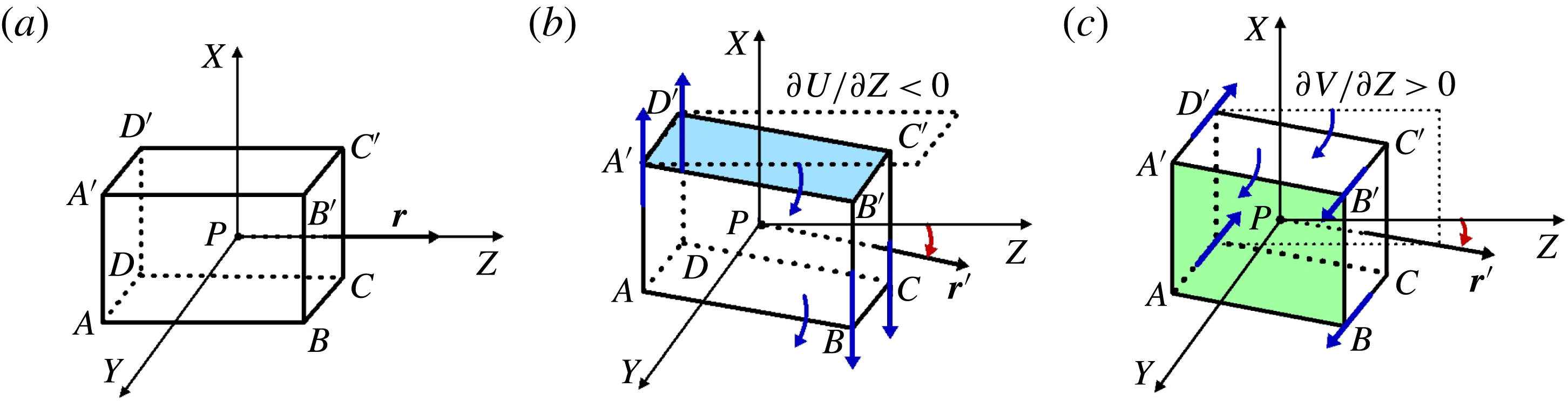
The methods to determine the local rotational axis will be studied in this section. Assume that there is an orthogonal coordinate system $XYZ$ with the origin at point $P$ (see figure 1 a), the following definitions and theorems can be given.

Figure 1.

Rotation of a 3-D fluid element centred at point $P$ in the reference frame $XYZ$ : (a) the fluid element at the initial time; (b) the surfaces $ABCD$ , $A^{\prime }B^{\prime }C^{\prime }D^{\prime }$ and the vector $\boldsymbol{r}$ will rotate around the $Y$ axis if $\unicode[STIX]{x2202}U/\unicode[STIX]{x2202}Z\neq 0$ ; (c) the surfaces $ABB^{\prime }A^{\prime }$ , $DCC^{\prime }D^{\prime }$ and vector $\boldsymbol{r}$ will rotate around the $X$ axis if $\unicode[STIX]{x2202}V/\unicode[STIX]{x2202}Z\neq 0$ .

From the above definitions and theorems, it can be concluded that if $Z$ is a local rotation axis at point $P$ , there must be $\unicode[STIX]{x2202}U/\unicode[STIX]{x2202}Z=0$ and $\unicode[STIX]{x2202}V/\unicode[STIX]{x2202}Z=0$ at point $P$ . However, the local rotation axis of a point in a general reference frame is not always parallel to the $Z$ axis. It can be determined by the transformation of the reference frame. Let us consider a point $P$ in a reference frame $xyz$ and assume that the local rotation axis of the point $P$ is a vector of $\boldsymbol{r}=r_{x}\boldsymbol{i}+r_{y}\,\boldsymbol{j}+r_{z}\boldsymbol{k}$ passing through the point $P$ . We transform the reference frame $xyz$ to a new reference frame $XYZ$ in which the fluid-rotational axis vector $\boldsymbol{r}$ is parallel to the axis $Z$ . The velocity gradient tensor $\unicode[STIX]{x1D735}\boldsymbol{v}$ and $\unicode[STIX]{x1D735}\boldsymbol{V}$ in reference frames $xyz$ and $XYZ$ can be written respectively as follows,

(2.1) $$\begin{eqnarray}\displaystyle \unicode[STIX]{x1D735}\boldsymbol{v}=\left[\begin{array}{@{}ccc@{}}\unicode[STIX]{x2202}u/\unicode[STIX]{x2202}x & \unicode[STIX]{x2202}u/\unicode[STIX]{x2202}y & \unicode[STIX]{x2202}u/\unicode[STIX]{x2202}z\\ \unicode[STIX]{x2202}v/\unicode[STIX]{x2202}x & \unicode[STIX]{x2202}v/\unicode[STIX]{x2202}y & \unicode[STIX]{x2202}v/\unicode[STIX]{x2202}z\\ \unicode[STIX]{x2202}w/\unicode[STIX]{x2202}x & \unicode[STIX]{x2202}w/\unicode[STIX]{x2202}y & \unicode[STIX]{x2202}w/\unicode[STIX]{x2202}z\end{array}\right] & & \displaystyle\end{eqnarray}$$

(2.2) $$\begin{eqnarray}\displaystyle \unicode[STIX]{x1D735}\boldsymbol{V}=\left[\begin{array}{@{}ccc@{}}\unicode[STIX]{x2202}U/\unicode[STIX]{x2202}X & \unicode[STIX]{x2202}U/\unicode[STIX]{x2202}Y & \unicode[STIX]{x2202}U/\unicode[STIX]{x2202}Z\\ \unicode[STIX]{x2202}V/\unicode[STIX]{x2202}X & \unicode[STIX]{x2202}V/\unicode[STIX]{x2202}Y & \unicode[STIX]{x2202}V/\unicode[STIX]{x2202}Z\\ \unicode[STIX]{x2202}W/\unicode[STIX]{x2202}X & \unicode[STIX]{x2202}W/\unicode[STIX]{x2202}Y & \unicode[STIX]{x2202}W/\unicode[STIX]{x2202}Z\end{array}\right]. & & \displaystyle\end{eqnarray}$$

The relation between the velocity gradient tensor in two reference frames can be written as

(2.3) $$\begin{eqnarray}\displaystyle \unicode[STIX]{x1D735}\boldsymbol{V}=\unicode[STIX]{x1D64C}\unicode[STIX]{x1D735}\boldsymbol{v}\unicode[STIX]{x1D64C}^{-1}, & & \displaystyle\end{eqnarray}$$

where $\unicode[STIX]{x1D64C}$ is the transformation matrix from frame $xyz$ to frame $XYZ$ , and by using the quaternions method (Katz Reference Katz1996), we can obtain

(2.4) $$\begin{eqnarray}\displaystyle \unicode[STIX]{x1D64C}=\left[\begin{array}{@{}ccc@{}}\displaystyle {\displaystyle \frac{r_{y}^{2}+r_{z}^{2}+r_{z}}{1+r_{z}}} & \displaystyle -{\displaystyle \frac{r_{x}r_{y}}{1+r_{z}}} & -r_{x}\\ \displaystyle -{\displaystyle \frac{r_{x}r_{y}}{1+r_{z}}} & \displaystyle \frac{r_{x}^{2}+r_{z}^{2}+r_{z}}{1+r_{z}} & -r_{y}\\ r_{x} & r_{y} & r_{z}\end{array}\right] & & \displaystyle\end{eqnarray}$$

and

(2.5) $$\begin{eqnarray}\displaystyle \unicode[STIX]{x1D64C}^{-1}=\unicode[STIX]{x1D64C}^{\text{T}}=\left[\begin{array}{@{}ccc@{}}\displaystyle \frac{r_{y}^{2}+r_{z}^{2}+r_{z}}{1+r_{z}} & \displaystyle -\frac{r_{x}r_{y}}{1+r_{z}} & r_{x}\\ \displaystyle -\frac{r_{x}r_{y}}{1+r_{z}} & \displaystyle \frac{r_{x}^{2}+r_{z}^{2}+r_{z}}{1+r_{z}} & r_{y}\\ -r_{x} & -r_{y} & r_{z}\end{array}\right], & & \displaystyle\end{eqnarray}$$

where $\boldsymbol{r}=r_{x}\boldsymbol{i}+r_{y}\,\boldsymbol{j}+r_{z}\boldsymbol{k}$ . The detailed derivation of the transformation matrix above is given in appendix A.

Base on the above conclusion, there must be $\unicode[STIX]{x2202}U/\unicode[STIX]{x2202}Z=0$ and $\unicode[STIX]{x2202}V/\unicode[STIX]{x2202}Z=0$ in the reference frame $XYZ$ if $\boldsymbol{r}=r_{x}\boldsymbol{i}+r_{y}\,\boldsymbol{j}+r_{z}\boldsymbol{k}$ in the frame $xyz$ is the direction of the local rotational axis. We can find vector $\boldsymbol{r}$ by solving the following equations,

(2.6) $$\begin{eqnarray}\displaystyle & \displaystyle {r_{x}}^{2}+{r_{y}}^{2}+{r_{z}}^{2}=1, & \displaystyle\end{eqnarray}$$

(2.7) $$\begin{eqnarray}\displaystyle & \displaystyle {\displaystyle \frac{\unicode[STIX]{x2202}U}{\unicode[STIX]{x2202}Z}}=0, & \displaystyle\end{eqnarray}$$

(2.8) $$\begin{eqnarray}\displaystyle & \displaystyle {\displaystyle \frac{\unicode[STIX]{x2202}V}{\unicode[STIX]{x2202}Z}}=0, & \displaystyle\end{eqnarray}$$

where $\unicode[STIX]{x2202}U/\unicode[STIX]{x2202}Z$ and $\unicode[STIX]{x2202}V/\unicode[STIX]{x2202}Z$ are determined by (2.3) in which $\unicode[STIX]{x1D735}\boldsymbol{v}$ is a known tensor. Therefore, $\unicode[STIX]{x2202}U/\unicode[STIX]{x2202}Z$ and $\unicode[STIX]{x2202}V/\unicode[STIX]{x2202}Z$ are the functions of the unite vector $\boldsymbol{r}$ . Based on the Schur decomposition theory (Gentle Reference Gentle1998), there must be an orthogonal matrix $\unicode[STIX]{x1D64C}$ which can make $\unicode[STIX]{x1D735}\boldsymbol{V}$ be a blocks-triangular matrix. Therefore, the solution of the set of equations (2.6)–(2.8) must exist. The formulas of (2.7) and (2.8) in terms of vector $\boldsymbol{r}$ are given in appendix B. The system of (2.6)–(2.8) is a set of nonlinear algebraic equations with the unknown vector $\boldsymbol{r}$ and it can be solved by using the Newton iterative method. As is well known, the efficiency of the Newton iterative method is dependent on the initial guess. If the initial guess is sufficiently close to the solution, the Newton iterative method will converge rather fast. We use the vorticity direction as the initial guess. The application example in § 4.3 will show that it works efficiently.

However, the condition that $\unicode[STIX]{x2202}U/\unicode[STIX]{x2202}Z=0$ and $\unicode[STIX]{x2202}V/\unicode[STIX]{x2202}Z=0$ in a reference frame by no means implies that there is a rotation around $Z$ axis. It only shows that the fluid has no rotation around the $X$ and $Y$ axes, or, in other words, that the fluid only has shear or/and deformation in the $X$ and $Y$ directions. Therefore, after we find the rotation axis which is a unit vector $\boldsymbol{r}$ , we should further determine if there is fluid rotation around the axis aligned with $\boldsymbol{r}$ at point $P$ , which can be distinguished by analysing the distributions of velocity derivatives in the normal plane $XY$ of vector $\boldsymbol{r}$ .

Figure 2.

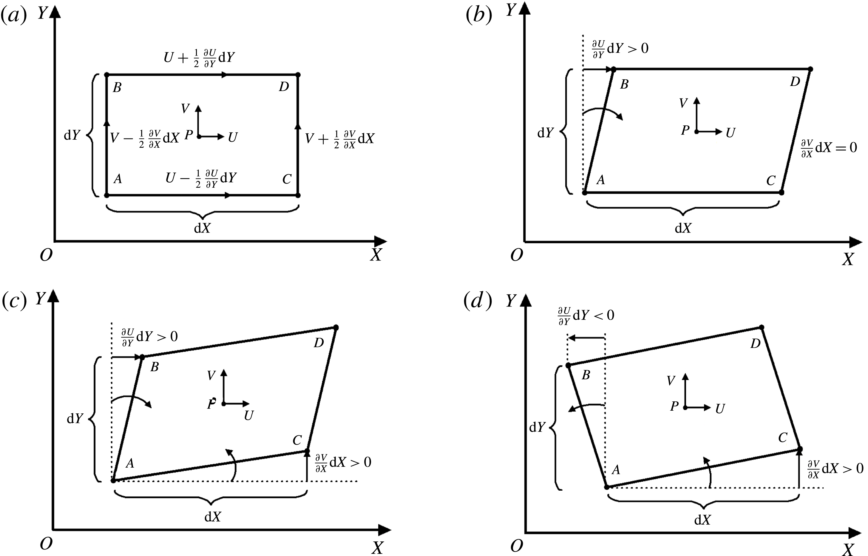
Rotation and distortion of a fluid element in 2-D plane. (a) Fluid element at time $t$ . (b) Pure shearing deformation. (c) Irrotational deformation. (d) Rotational deformation.

2.2 Rotation strength in the 2-D plane perpendicular to the local rotation axis

Let us first consider an infinitesimal fluid element moving in a two-dimensional flow of the $XY$ plane. At time $t$ , the shape of this fluid element centred at position $P$ is rectangular and we can assume, without losing generality, that the fluid element is moving upward and from the left to right, as shown in figure 2(a). After a time increment $\unicode[STIX]{x0394}t$ , its position and shape may change, which is determined by the distribution of velocity and its gradient tensor. In the following analysis, we will ignore the translation of the fluid element. Hence, in the $XY$ plane of reference frame $XYZ$ , side $AB$ of the rectangular fluid element will have a clockwise rotation if $\unicode[STIX]{x2202}U/\unicode[STIX]{x2202}Y>0$ , or have a counter-clockwise rotation if $\unicode[STIX]{x2202}U/\unicode[STIX]{x2202}Y<0$ and have no rotation if $\unicode[STIX]{x2202}U/\unicode[STIX]{x2202}Y=0$ . Side $AC$ will have a counter-clockwise rotation if $\unicode[STIX]{x2202}V/\unicode[STIX]{x2202}X>0$ , have a clockwise rotation if $\unicode[STIX]{x2202}V/\unicode[STIX]{x2202}X<0$ and have no rotation if $\unicode[STIX]{x2202}V/\unicode[STIX]{x2202}X=0$ . In classic fluid dynamics, the angular velocity of fluid element is defined as half of the vorticity, which is $\unicode[STIX]{x2202}V/\unicode[STIX]{x2202}X-\unicode[STIX]{x2202}U/\unicode[STIX]{x2202}Y$ in 2-D flow. It is easily found that there is a non-zero angular velocity or vorticity when $\unicode[STIX]{x2202}V/\unicode[STIX]{x2202}X\neq \unicode[STIX]{x2202}U/\unicode[STIX]{x2202}Y$ , but this does not mean that the fluid always has a rotation. For instance, it only has a pure shearing in the case of figure 2(b) with $\unicode[STIX]{x2202}V/\unicode[STIX]{x2202}X=0$ and irrotational deformation in the case of figure 2(c) when $\unicode[STIX]{x2202}V/\unicode[STIX]{x2202}X>0$ and $\unicode[STIX]{x2202}U/\unicode[STIX]{x2202}Y>0$ . In this paper, we think the element in the reference frame $XY$ has a rotational motion only when the two sides of $AB$ and $AC$ have a same rotational direction, as shown in figure 2(d) with $\unicode[STIX]{x2202}V/\unicode[STIX]{x2202}X>0$ and $\unicode[STIX]{x2202}U/\unicode[STIX]{x2202}Y<0$ . Generally, we can judge the motion of a fluid element in a reference frame by the following criterion,

(2.9) $$\begin{eqnarray}\displaystyle & \displaystyle g_{Z}=-{\displaystyle \frac{\unicode[STIX]{x2202}V}{\unicode[STIX]{x2202}X}}\frac{\unicode[STIX]{x2202}U}{\unicode[STIX]{x2202}Y} & \displaystyle\end{eqnarray}$$

(i) pure shearing or no deformation if $g_{Z}=0$ ;

(ii) irrotational deformation if $g_{Z}<0$ ;

(iii) rotational deformation if $g_{Z}>0$ .

As is known, vorticity $\unicode[STIX]{x1D709}_{Z}=\unicode[STIX]{x2202}V/\unicode[STIX]{x2202}X-\unicode[STIX]{x2202}U/\unicode[STIX]{x2202}Y$ in a 2-D flow is a invariant quantity, which means that $\unicode[STIX]{x1D709}_{Z}$ does not change with the rotation of the plane $XY$ around the $Z$ axis. However, $\unicode[STIX]{x2202}V/\unicode[STIX]{x2202}X$ or $\unicode[STIX]{x2202}U/\unicode[STIX]{x2202}Y$ is not invariant and will change with the rotation of the reference frame. When frame $XYZ$ is rotated around the $Z$ axis by an angle $\unicode[STIX]{x1D703}$ , the new velocity gradient tensor is

(2.10) $$\begin{eqnarray}\displaystyle \unicode[STIX]{x1D735}\boldsymbol{V}_{\unicode[STIX]{x1D703}}=\unicode[STIX]{x1D64B}\unicode[STIX]{x1D735}\boldsymbol{V}\unicode[STIX]{x1D64B}^{-1}, & & \displaystyle\end{eqnarray}$$

where $\unicode[STIX]{x1D64B}$ is the transformation matrix around axis $Z$ and there are

(2.11) $$\begin{eqnarray}\displaystyle \unicode[STIX]{x1D64B}=\left[\begin{array}{@{}ccc@{}}\cos \unicode[STIX]{x1D703} & \sin \unicode[STIX]{x1D703} & 0\\ -\text{sin}\,\unicode[STIX]{x1D703} & \cos \unicode[STIX]{x1D703} & 0\\ 0 & 0 & 1\end{array}\right] & & \displaystyle\end{eqnarray}$$

and

(2.12) $$\begin{eqnarray}\displaystyle \unicode[STIX]{x1D64B}^{-1}=\unicode[STIX]{x1D64B}^{\text{T}}=\left[\begin{array}{@{}ccc@{}}\cos \unicode[STIX]{x1D703} & -\text{sin}\,\unicode[STIX]{x1D703} & 0\\ \sin \unicode[STIX]{x1D703} & \cos \unicode[STIX]{x1D703} & 0\\ 0 & 0 & 1\end{array}\right]. & & \displaystyle\end{eqnarray}$$

So, we can obtain

(2.13) $$\begin{eqnarray}\displaystyle & \displaystyle \left.{\displaystyle \frac{\unicode[STIX]{x2202}V}{\unicode[STIX]{x2202}X}}\right|_{\unicode[STIX]{x1D703}}=\unicode[STIX]{x1D6FC}\sin (2\unicode[STIX]{x1D703}+\unicode[STIX]{x1D719})+\unicode[STIX]{x1D6FD}, & \displaystyle\end{eqnarray}$$

(2.14) $$\begin{eqnarray}\displaystyle & \displaystyle \left.{\displaystyle \frac{\unicode[STIX]{x2202}U}{\unicode[STIX]{x2202}Y}}\right|_{\unicode[STIX]{x1D703}}=\unicode[STIX]{x1D6FC}\sin (2\unicode[STIX]{x1D703}+\unicode[STIX]{x1D719})-\unicode[STIX]{x1D6FD}, & \displaystyle\end{eqnarray}$$

where

(2.15) $$\begin{eqnarray}\displaystyle & \displaystyle \unicode[STIX]{x1D6FC}={\displaystyle \frac{1}{2}}\sqrt{\left({\displaystyle \frac{\unicode[STIX]{x2202}U}{\unicode[STIX]{x2202}X}}-{\displaystyle \frac{\unicode[STIX]{x2202}V}{\unicode[STIX]{x2202}Y}}\right)^{2}+\left({\displaystyle \frac{\unicode[STIX]{x2202}V}{\unicode[STIX]{x2202}X}}+{\displaystyle \frac{\unicode[STIX]{x2202}U}{\unicode[STIX]{x2202}Y}}\right)^{2}}, & \displaystyle\end{eqnarray}$$

(2.16) $$\begin{eqnarray}\displaystyle & \displaystyle \unicode[STIX]{x1D6FD}={\displaystyle \frac{1}{2}}\left({\displaystyle \frac{\unicode[STIX]{x2202}V}{\unicode[STIX]{x2202}X}}-{\displaystyle \frac{\unicode[STIX]{x2202}U}{\unicode[STIX]{x2202}Y}}\right) & \displaystyle\end{eqnarray}$$

and

(2.17) $$\begin{eqnarray}\displaystyle & \displaystyle \unicode[STIX]{x1D719}=\displaystyle {\displaystyle \frac{\displaystyle \frac{\unicode[STIX]{x2202}V}{\unicode[STIX]{x2202}X}+\displaystyle \frac{\unicode[STIX]{x2202}U}{\unicode[STIX]{x2202}Y}}{\displaystyle \frac{\unicode[STIX]{x2202}V}{\unicode[STIX]{x2202}Y}-\displaystyle \frac{\unicode[STIX]{x2202}U}{\unicode[STIX]{x2202}X}}}. & \displaystyle\end{eqnarray}$$

Based on (2.13) and (2.14), the criterion of rotation of a fluid element in (2.9) becomes

(2.18) $$\begin{eqnarray}\displaystyle & \displaystyle g_{Z\unicode[STIX]{x1D703}}=\left.-{\displaystyle \frac{\unicode[STIX]{x2202}V}{\unicode[STIX]{x2202}X}}\right|_{\unicode[STIX]{x1D703}}\left.{\displaystyle \frac{\unicode[STIX]{x2202}U}{\unicode[STIX]{x2202}Y}}\right|_{\unicode[STIX]{x1D703}}=\unicode[STIX]{x1D6FD}^{2}-\unicode[STIX]{x1D6FC}^{2}\sin ^{2}(2\unicode[STIX]{x1D703}+\unicode[STIX]{x1D719}). & \displaystyle\end{eqnarray}$$

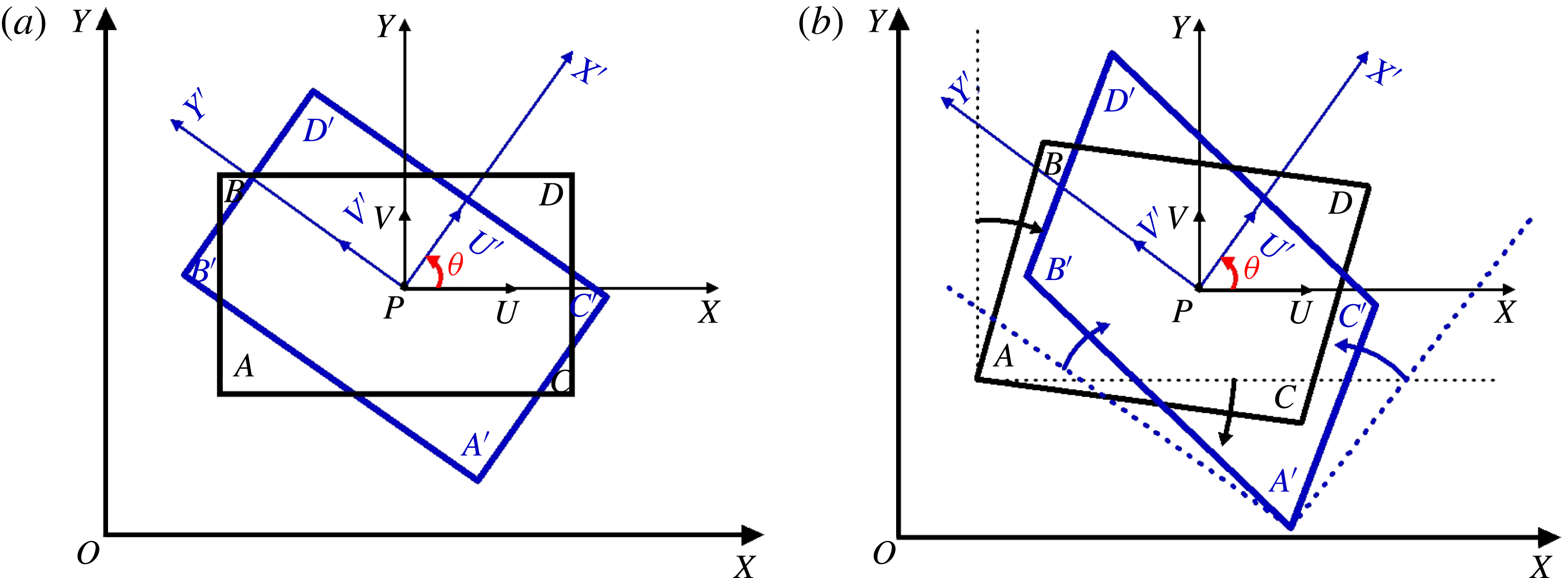
It can be seen that the sign of $g_{Z\unicode[STIX]{x1D703}}$ will change with the azimuthal angle $\unicode[STIX]{x1D703}$ if $\unicode[STIX]{x1D6FC}^{2}>\unicode[STIX]{x1D6FD}^{2}$ . This implies that at the same point $P$ , the fluid elements at different azimuthal angles may have different types of motion as we look at the fluid motion in different reference frames, which means that the rotation type (clockwise or counter-clockwise) is not invariant. For example, as shown in figure 3(a), for the same point $P$ , we can consider two different fluid elements in two different frames. After a time increment $\unicode[STIX]{x0394}t$ , the fluid element in $XY$ has a rotational deformation $g_{Z}>0$ , see black element in figure 3(b). However, the fluid element, centred at the same point $P$ but in a frame rotated by an angle $\unicode[STIX]{x1D703}$ , has an irrotational deformation as $g_{Z}<0$ , see blue element in figure 3(b). This reveals that the motion character of the fluid element centred at a point is related to the azimuthal angle $\unicode[STIX]{x1D703}$ , or, in other words, the motion is not invariant when looking in different reference frames when $\unicode[STIX]{x1D6FC}^{2}>\unicode[STIX]{x1D6FD}^{2}$ . However, if $\unicode[STIX]{x1D6FC}^{2}<\unicode[STIX]{x1D6FD}^{2}$ , $g_{Z\unicode[STIX]{x1D703}}>0$ for any $\unicode[STIX]{x1D703}\in [0,2\unicode[STIX]{x03C0})$ , which means that the fluid element at any reference frame has the same rotation direction. In this paper, we consider that a point is fluid rotational if the rotation direction is invariant in any reference frame. Therefore, based on the distribution of the criterion $g_{Z\unicode[STIX]{x1D703}}$ , we propose a definition to identify if a point is fluid rotational or non-rotational in a 2-D plane as follows,

Figure 3.

Rotation character of a fluid element in two different reference frames. (a) Rectangular fluid element at time $t$ . (b) Rotation and distortion after a time increment $\unicode[STIX]{x0394}t$ .

Definition 3. A point is local fluid rotational if the velocity gradient tensor at the point meets

(2.19) $$\begin{eqnarray}\displaystyle & \displaystyle g_{Zmin}=g_{Z\unicode[STIX]{x1D703}min}=\unicode[STIX]{x1D6FD}^{2}-\unicode[STIX]{x1D6FC}^{2}>0, & \displaystyle\end{eqnarray}$$

where $\unicode[STIX]{x1D6FC}$ and $\unicode[STIX]{x1D6FD}$ are defined in (2.15) and (2.16).

This definition implies that if a point is fluid rotational, in any 2-D reference frames, the fluid element has a rotational motion and the rotational direction is invariant. In other words, the fluid at any azimuthal angle $\unicode[STIX]{x1D703}$ around the point has the same rotation direction relative to the point. From the (2.13), $\unicode[STIX]{x2202}V/\unicode[STIX]{x2202}X$ can be regarded as the angular velocity of the fluid at azimuthal angle $\unicode[STIX]{x1D703}$ relative to the point, so we have

(2.20) $$\begin{eqnarray}\displaystyle & \displaystyle \unicode[STIX]{x1D714}_{\unicode[STIX]{x1D703}}=\left.{\displaystyle \frac{\unicode[STIX]{x2202}V}{\unicode[STIX]{x2202}X}}\right|_{\unicode[STIX]{x1D703}}=\unicode[STIX]{x1D6FC}\sin (2\unicode[STIX]{x1D703}+\unicode[STIX]{x1D719})+\unicode[STIX]{x1D6FD}. & \displaystyle\end{eqnarray}$$

It can be easily obtained from (2.20) that the direction of angular velocity is invariant for the fluid-rotational point, but it is not for the non-fluid-rotational point. Different from the rotation of rigid body which has the same angular velocity for every point, the angular velocity of a fluid, even if at the same point, changes with the azimuthal angle. The fluid-rotational angular velocity for a fluid-rotational point in the 2-D plane is defined as the minimum angular velocity of (2.20). However, the fluid-rotational angular velocity of a point is 0 if it is not fluid rotational. Without loss of generality, assume $\unicode[STIX]{x1D6FD}>0$ (if $\unicode[STIX]{x1D6FD}<0$ , we can change the direction of the local rotation axis to make sure $\unicode[STIX]{x1D6FD}>0$ ) and the fluid-rotational angular velocity at a point can be determined as

(2.21) $$\begin{eqnarray}\displaystyle \unicode[STIX]{x1D714}_{rot}=\unicode[STIX]{x1D714}_{\unicode[STIX]{x1D703}min}\left\{\begin{array}{@{}ll@{}}\unicode[STIX]{x1D6FD}-\unicode[STIX]{x1D6FC}, & g_{Zmin}>0,\\[12.0pt] 0, & g_{Zmin}\leqslant 0.\end{array}\right. & & \displaystyle\end{eqnarray}$$

Similar to the definition of vorticity, which is twice the average angular velocity of the rectangle element, in a 2-D plane, we define the vortex vector which is the rotational part as twice the fluid-rotational angular velocity,

(2.22) $$\begin{eqnarray}\displaystyle R_{Z}=2\unicode[STIX]{x1D714}_{rot}. & & \displaystyle\end{eqnarray}$$

In fact, it can be seen from (2.16) that $\unicode[STIX]{x1D6FD}$ is the average angular velocity of the fluid element or half of the vorticity in the $Z$ direction. Therefore, based on (2.15), (2.16), (2.21) and (2.22), we can obtain

(2.23) $$\begin{eqnarray}\displaystyle \unicode[STIX]{x1D709}_{Z}=R_{Z}+S_{Z}, & & \displaystyle\end{eqnarray}$$

where $\unicode[STIX]{x1D709}_{Z}=2\unicode[STIX]{x1D6FD}=(\unicode[STIX]{x2202}V/\unicode[STIX]{x2202}X)-(\unicode[STIX]{x2202}U/\unicode[STIX]{x2202}Y)$ is the vorticity and $S_{Z}=2\unicode[STIX]{x1D6FC}=$ $\sqrt{\left((\unicode[STIX]{x2202}U/\unicode[STIX]{x2202}X)-(\unicode[STIX]{x2202}V/\unicode[STIX]{x2202}Y)\right)^{2}+\left((\unicode[STIX]{x2202}V/\unicode[STIX]{x2202}X)+(\unicode[STIX]{x2202}U/\unicode[STIX]{x2202}Y)\right)^{2}}$ is the non-rotational part of the vorticity which is the shear or/and deformation in the $Z$ direction.

3.1 Definition of vortex vector

In § 2, by analysing the physical meaning of the motion of the fluid element in 3-D and 2-D flows, we present several concepts, such as the local rotation axis, the local rotation plane and the local fluid rotation. By these concepts and definitions, we will propose a definition of a new vector quantity which is called the vortex vector. In this paper, the new vector quantity will be used to definite the vortex.

Definition 4. A vortex vector $\boldsymbol{R}$ at a point is a vector quantity which represents the local fluid rotation and is defined as

(3.1) $$\begin{eqnarray}\displaystyle \boldsymbol{R}=R_{Z}\boldsymbol{r}. & & \displaystyle\end{eqnarray}$$

3.2 Decomposition of vorticity

As Liu et al. (Reference Liu, Wang, Yang and Duan2016) addressed, the vorticity can be further decomposed into a rotational part and a non-rotational part. As shown in § 2, there is only shear and deformation in the direction perpendicular to $\boldsymbol{R}$ and the vortex vector is the rotational part of the vorticity in the $\boldsymbol{R}$ direction. So, after finding the rotational part of vorticity, we can easily obtain the non-rotational part of the vorticity $\boldsymbol{S}$ which is a pure shear and deformation of fluid by

(3.2) $$\begin{eqnarray}\displaystyle \boldsymbol{S}=\unicode[STIX]{x1D735}\times \boldsymbol{v}-\boldsymbol{R}. & & \displaystyle\end{eqnarray}$$

The vortex vector $\boldsymbol{R}$ represents the rotation of the fluid and the non-rotational part of the vorticity $\boldsymbol{S}$ represents the shear or/and deformation of the fluid.

3.3 Definition of a vortex

In the above subsection, we give a new vector quantity, the vortex vector, whose direction is that of the fluid-rotation axis and whose magnitude is the strength of the fluid rotation. The vortex vector can be used to define a vortex, which is the building block of the turbulence coherent structure, as follows

After defining a vortex, visualizing the vertical structure in the flow field is still a problem. Similar to the vorticity line and vorticity tube, the vortex line and vortex tube can be developed to display the vortical structures. A vortex line is a curve whose tangent at any point is in the direction of the vortex vector at that point. The concept of the vortex tube is related to the vortex line. Consider an arbitrary closed curve in three-dimensional space, the vortex lines which pass through all points on the curve form a tube in space and such a tube is called a vortex tube.

Since we have defined the vortex vector, we have two different ways to describe the vortex structure in a flow field: using vortex lines and tubes or using the iso-surface of the magnitude of the vortex vector which represents the strength of fluid rotation. In the next section we will demonstrate the capability of the vortex vector in describing the complex vortex structure in different flow fields. Mainly, we will use the iso-surface of the vortex strength while leaving the vortex lines and tubes for future applications. It must be pointed out that one of the main differences between the current vortex vector definition and all other vortex identification methods is that the current vortex vector definition is a vector but the others are scalars. Therefore, this definition can use both iso-surface and vortex line/tube/surface to discover the vertical structure, while others can only use a criterion or threshold to display iso-surfaces.

4.1 Verification of the simple motion models

To verify the definitions presented in §§ 2 and 3, two examples are used: (i) rigid-body rotation; (ii) Blasius solution of a laminar boundary layer.

4.1.1 Rigid-body rotation

The motion of a rigid body can be described by a translation of the centre of mass and a rotation around the centre of mass. By choosing a reference frame moving with the centre of mass, all elements of the rigid body are rotating around the centre of mass with the same angular speed. Without loss of generality, the velocity of a rigid body in the moving reference frame whose axis $Z$ coincides with the rotation axis can be written as

(4.1a-c ) $$\begin{eqnarray}\displaystyle u=\unicode[STIX]{x1D714}y,\quad v=-\unicode[STIX]{x1D714}x,\quad w=0. & & \displaystyle\end{eqnarray}$$

As there are $\unicode[STIX]{x2202}u/\unicode[STIX]{x2202}z=0$ and $\unicode[STIX]{x2202}v/\unicode[STIX]{x2202}z=0$ at every point in this velocity field, based on the Theorem 2, the local rotation axis is parallel to the axis $z$ . The vortex vector can be obtained as

(4.2) $$\begin{eqnarray}\displaystyle & \displaystyle \boldsymbol{R}=2\left(\unicode[STIX]{x1D6FD}-\unicode[STIX]{x1D6FC}\right)\boldsymbol{k}=\left[\left({\displaystyle \frac{\unicode[STIX]{x2202}v}{\unicode[STIX]{x2202}x}}-{\displaystyle \frac{\unicode[STIX]{x2202}u}{\unicode[STIX]{x2202}y}}\right)-\sqrt{\left({\displaystyle \frac{\unicode[STIX]{x2202}u}{\unicode[STIX]{x2202}x}}-\frac{\unicode[STIX]{x2202}v}{\unicode[STIX]{x2202}y}\right)^{2}+\left({\displaystyle \frac{\unicode[STIX]{x2202}v}{\unicode[STIX]{x2202}x}}+{\displaystyle \frac{\unicode[STIX]{x2202}u}{\unicode[STIX]{x2202}y}}\right)^{2}}\right]\boldsymbol{k}=2\unicode[STIX]{x1D714}\boldsymbol{k}.\qquad & \displaystyle\end{eqnarray}$$

This means that the vortex vector is twice the angular speed of rigid body rotation. The vorticity at every point can be given as

(4.3) $$\begin{eqnarray}\displaystyle \unicode[STIX]{x1D743}=\unicode[STIX]{x1D735}\times \boldsymbol{v}=2\unicode[STIX]{x1D714}\boldsymbol{k}. & & \displaystyle\end{eqnarray}$$

Therefore, for the rotation of the rigid body, $\boldsymbol{R}=\unicode[STIX]{x1D735}\times \boldsymbol{v}$ and $\boldsymbol{S}=\unicode[STIX]{x1D735}\times \boldsymbol{v}-\boldsymbol{R}=0$ . There is no shear and deformation in the rigid-body rotation and this is the physical character of the rigid-body motion.

4.1.2 Blasius solution of laminar boundary layer

The 2-D laminar boundary layer can be described as the Blasius solution and the velocity can be written as

(4.4a-c ) $$\begin{eqnarray}\displaystyle u=U(y),\quad v=0,\quad w=0. & & \displaystyle\end{eqnarray}$$

By Theorem 2 and (2.6)–(2.7), there are two possible local rotation axis, e.g. the $x$ axis and $z$ axis, as $\unicode[STIX]{x2202}v/\unicode[STIX]{x2202}x=0$ , $\unicode[STIX]{x2202}w/\unicode[STIX]{x2202}x=0$ and $\unicode[STIX]{x2202}u/\unicode[STIX]{x2202}z=0$ , $\unicode[STIX]{x2202}v/\unicode[STIX]{x2202}z=0$ . Based on the Definitions 3 and 4, the vortex vector can be valued as

(4.5) $$\begin{eqnarray}\displaystyle & \displaystyle \boldsymbol{R}=2\left(\unicode[STIX]{x1D6FD}-\unicode[STIX]{x1D6FC}\right)\boldsymbol{i}=\left[\left({\displaystyle \frac{\unicode[STIX]{x2202}w}{\unicode[STIX]{x2202}y}}-{\displaystyle \frac{\unicode[STIX]{x2202}v}{\unicode[STIX]{x2202}z}}\right)-\sqrt{\left({\displaystyle \frac{\unicode[STIX]{x2202}v}{\unicode[STIX]{x2202}y}}-{\displaystyle \frac{\unicode[STIX]{x2202}w}{\unicode[STIX]{x2202}z}}\right)^{2}+\left({\displaystyle \frac{\unicode[STIX]{x2202}w}{\unicode[STIX]{x2202}y}}+{\displaystyle \frac{\unicode[STIX]{x2202}v}{\unicode[STIX]{x2202}z}}\right)^{2}}\,\right]\boldsymbol{i}=0\qquad & \displaystyle\end{eqnarray}$$

or

(4.6) $$\begin{eqnarray}\displaystyle & \displaystyle \boldsymbol{R}=2\left(\unicode[STIX]{x1D6FD}-\unicode[STIX]{x1D6FC}\right)\boldsymbol{k}=\left[\left({\displaystyle \frac{\unicode[STIX]{x2202}v}{\unicode[STIX]{x2202}x}}-\frac{\unicode[STIX]{x2202}u}{\unicode[STIX]{x2202}y}\right)-\sqrt{\left({\displaystyle \frac{\unicode[STIX]{x2202}u}{\unicode[STIX]{x2202}x}}-{\displaystyle \frac{\unicode[STIX]{x2202}v}{\unicode[STIX]{x2202}y}}\right)^{2}+\left({\displaystyle \frac{\unicode[STIX]{x2202}v}{\unicode[STIX]{x2202}x}}+{\displaystyle \frac{\unicode[STIX]{x2202}u}{\unicode[STIX]{x2202}y}}\right)^{2}}\,\right]\boldsymbol{k}=0.\qquad & \displaystyle\end{eqnarray}$$

The vortex vector is 0 in the laminar boundary layer flow, which means that there is no rotation or vortex in the flow field. However, the distribution of vorticity in the velocity field is

(4.7) $$\begin{eqnarray}\displaystyle & \displaystyle \unicode[STIX]{x1D743}=\unicode[STIX]{x1D735}\times \boldsymbol{v}=-{\displaystyle \frac{\unicode[STIX]{x2202}U}{\unicode[STIX]{x2202}y}}\boldsymbol{k}. & \displaystyle\end{eqnarray}$$

Therefore, in the laminar boundary layer, there are $\boldsymbol{R}=0$ and $\boldsymbol{S}=\unicode[STIX]{x1D735}\times \boldsymbol{v}$ and there is only pure shear. The conclusion is the same as the current understanding of laminar flow.

From the examples above, it is clear that vorticity cannot really represent the rotation of the fluid, so it cannot fully describe the vortex. It should be further quantitatively decomposed into a rotational part (vortex vector) and non-rotational part (shear or/and deformation). Therefore, only the vortex vector can represent the rotation of the fluid. We will further investigate the vortex vector on describing the complex vortical structures of the DNS/LES databases.

4.2 Two-dimensional Blasius-profile temporal mixing layer flow

As the first DNS example, we consider a 2-D mirrored Blasius-profile shear layer excited with a perturbation to induce the rollup of the shear layer and the formation of vortices. The $Re$ , which is based on the displacement thickness, is 1000 and the inflow $Ma$ is $0.5$ . The unsteady 2-D flow field is numerically simulated by the code ‘DNSUTA’ in which the Navier–Stokes (NS) equations are solved using a sixth-order compact scheme in the spatial discretization and a third-order total variation diminishing (TVD) Runge–Kutta scheme in the temporal discretization. A local refined grid is generated with dimensions $256\times 512$ in the streamwise and normal directions respectively.

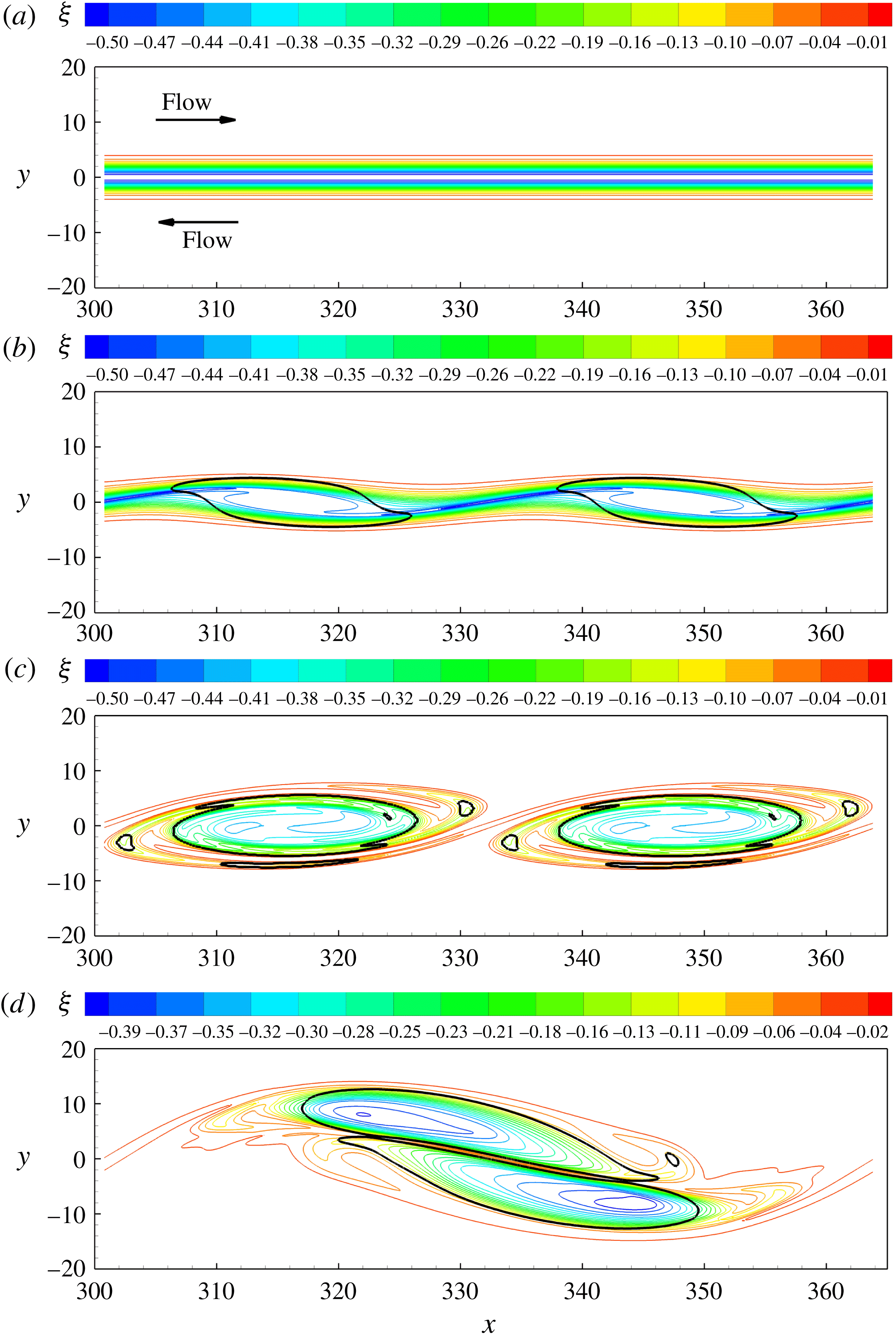
The evolution of the flow visualized by vorticity contours is shown in figure 4 for four time instants. At the initial stage, there is a large vortcity distribution in the shear layer, but the vortex vector $\boldsymbol{R}$ does not show up anywhere in the shear layer (see figure 4 a). This clearly implies that the existence of vorticity does not mean the existence of fluid rotation or vortex and the vorticity is not able to fully describe the vortex structure of the flow. In the following instants, two clockwise vortices appeared, which are shown as the black iso-line of the vortex vector $|\boldsymbol{R}|=0$ in figure 4(b–d) and the strength of the vortices become stronger as time advances.

Figure 4.

The temporal evolution of the shear layer. (a) The distributions of vorticity at the initial stage. (b) Vorticity distribution with weak vortex generated during shear layer rolling up. (c) Contours of vorticity with a pair of vortices generated. (d) Contours of vorticity in the paring of the two vortices.

Figure 5.

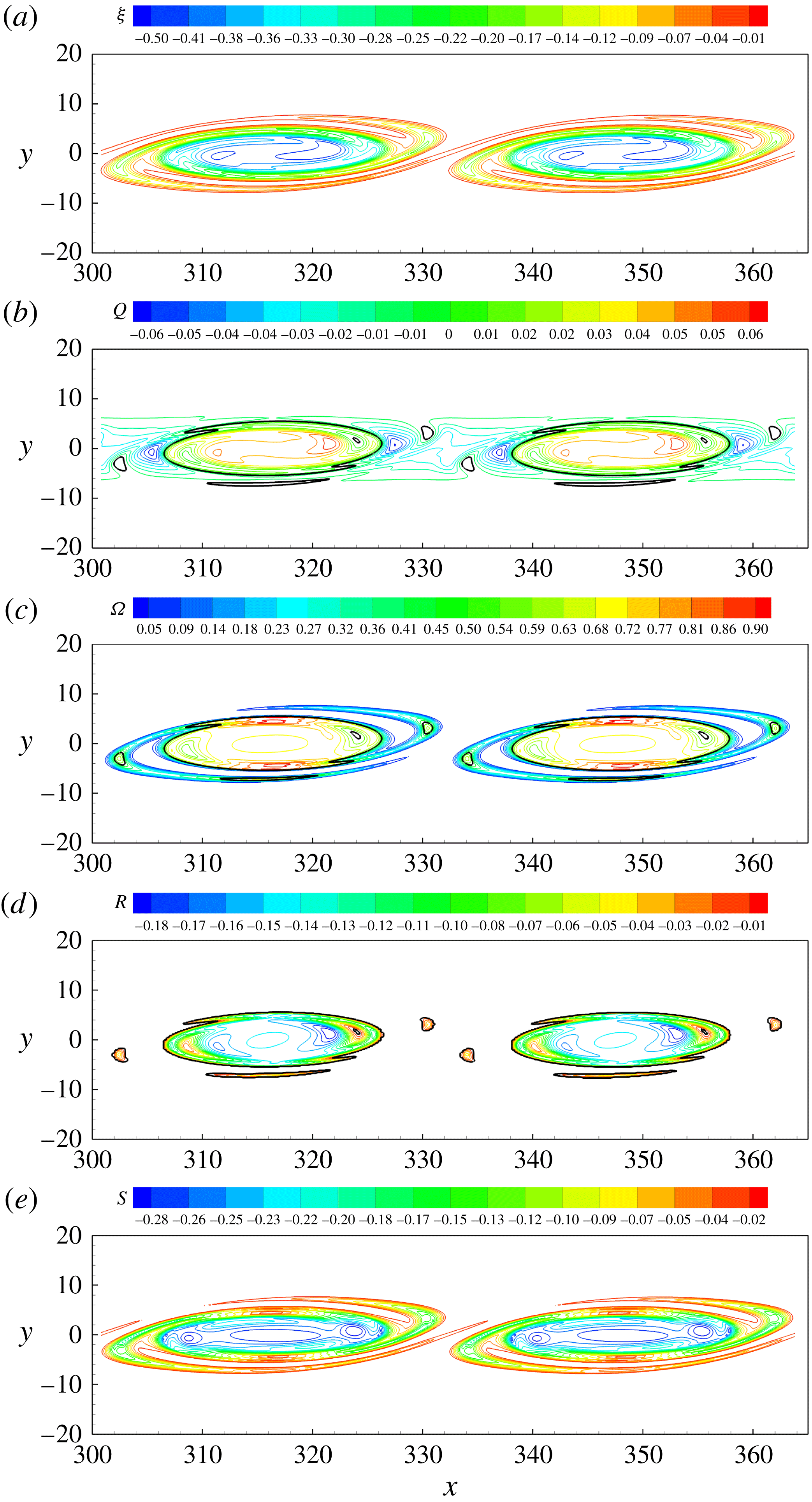
Distributions of a pair of vortices: (a) contours of vorticity for which it is not able to tell where the vortices are; (b) contours of $Q$ -criterion with the boundary of the vortex as the black lines which are the iso-lines of $Q=0.0$ ; (c) contours of $\unicode[STIX]{x1D6FA}$ -criterion with the boundary of the vortex as the black lines which are the iso-lines of $\unicode[STIX]{x1D6FA}=0.5$ ; (d) contours of the vortex vector with natural vortex boundaries which are the iso-lines of $|\boldsymbol{R}|=0$ ; (e) contours of the non-rotational part of the vorticity.

The vortices of the instantaneous flow field shown in figure 4(c) are identified by the $Q$ -criterion, $\unicode[STIX]{x1D6FA}$ -criterion and vortex vector $\boldsymbol{R}$ , respectively. The iso-lines of $Q$ , $\unicode[STIX]{x1D6FA}$ and $\boldsymbol{R}$ are shown in figure 5. In figure 5(a–c), the black lines are the boundaries of the vortices identified by $Q=0.0$ , $\unicode[STIX]{x1D6FA}=0.5$ and $|\boldsymbol{R}|=0$ , respectively. It can be seen that all those methods can give the same vortical structures in the 2-D low speed flow. In fact, we can obtain the same equation by substituting the continuity equation for 2-D incompressible flow into (2.19) which will become the $Q$ -criterion. Note that $|\boldsymbol{R}|$ and $Q$ are not same for 3-D flow or compressible flow. Figure 5(d) shows the distribution of the non-rotational part of the vorticity which describes the shearing of the flow. It can be seen that the distribution of the non-rotational part of the vorticity is very similar to that of the vorticity. This reveals that the fluid rotation is different from the rotation of the rigid body and there is a strong shearing conjugated with the rotation of fluids in the vortex.

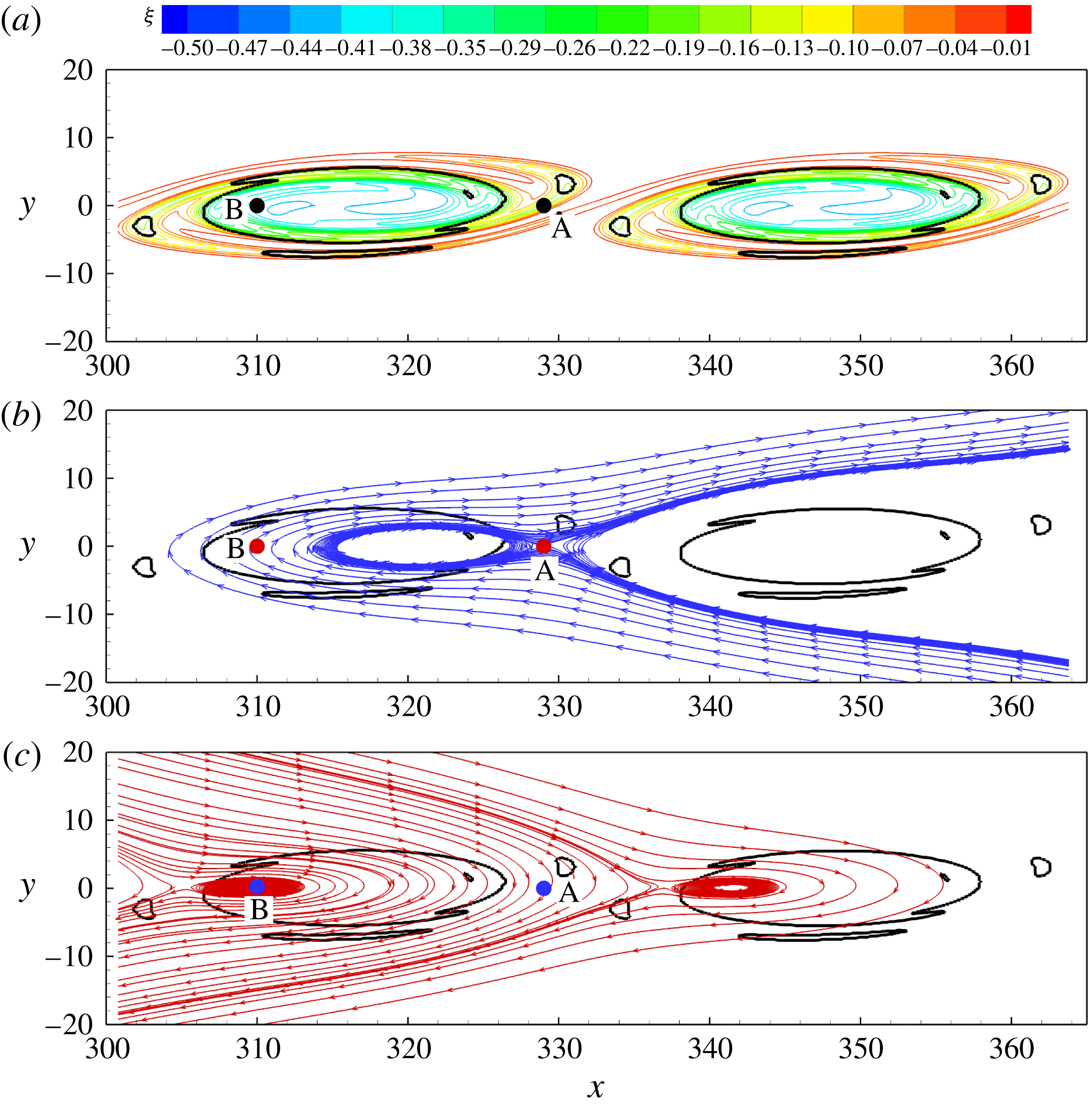
As we present in § 2, if a point in a flow field is fluid rotational, the fluid in the small neighbourhood of the point has the same tendency moving around it and pseudo-closed streamlines based on the velocity relative to the point can be created. At the instant shown in figure 4(c), we consider two points $A$ and $B$ , as shown in figure 6. Point $A$ is outside of the regions of the vortices and point $B$ lies in the left vortex, see figure 6(a). Using the velocity relative to each point respectively, the streamlines are created near point $A$ (see figure 6 b) and point $B$ (see figure 6 c). As we can see, there is no pseudo-closed streamline around point $A$ , but a pseudo-closed streamline can be formed around point $B$ , which shows that point $B$ is fluid rotational and point $A$ is not.

Figure 6.

Pseudo-streamlines based on the relative velocity. (a) The positions of point $A$ , which is out of the vortex, and point $B$ , which is inside the vortex. (b) No closed pseudo-streamline around non-fluid-rotational point $A$ . (c) Closed pseudo-streamline around the fluid-rotational point $B$ .

From this example, it can be seen that the definition of the vortex vector can precisely describe the vortex and its magnitude represents the strength of the vortex. In the vortex, each point is fluid rotational, which means that the fluid in the neighbourhood of that point has the same direction of tangential velocity relative to that point. As a newly defined vector quantity, the vortex vector can be used to quantitatively study vortices.

4.3 Vortices in late boundary layer flow transition

For 2-D vortical structures, the direction of the vortex vector is predetermined, which is vortical to the flow plane. However, in the 3-D flow, the directions of vortex cores are unknown and they may change in time and space. By the definition of the vortex vector, how to determine the vortex direction is a key issue. As another example, we consider the vortices in late boundary layer transition, which is a process of vortex ‘build-up’. In the process of boundary layer transition, a $\unicode[STIX]{x1D6EC}$ -shaped vortex and hairpin vortex can be commonly observed not only in the experiment but also in the DNS simulation and they will be used to show the ability of the newly defined vortex vector in representing the complex vortical structure. In the following, the DNS data (Liu et al. Reference Liu, Yan and Lu2014) of a late boundary layer flow transition obtained by DNSUTA are applied to capture the structures of the vortices.

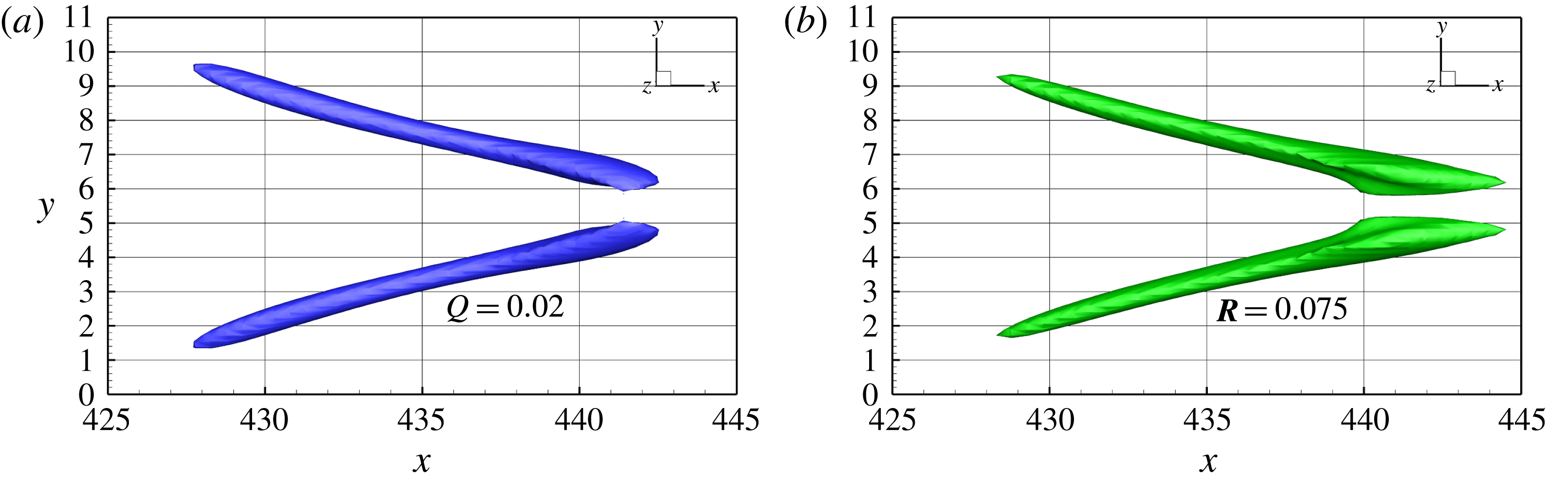
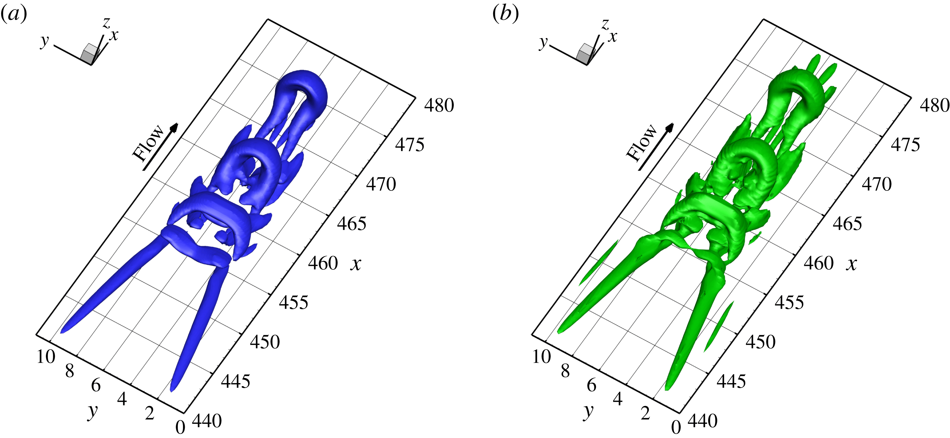
As one of the most popular vortex identification methods, the $Q$ -criterion is selected to compare the ability of capturing the vortical structures in turbulence with our newly defined vortex vector. In fluid dynamics, the iso-surface of $Q$ is always used to illustrate the cores of the vortex. The typical structure of a $\unicode[STIX]{x1D6EC}$ vortex is illustrated in figure 7 where the left blue surface is the iso-surface of $Q=0.02$ and the right green surface is the iso-surface of the magnitude of the vortex vector $|\boldsymbol{R}|=0.075$ . Both of them can illustrate the similar structure of the vortex cores. However, being different from the $Q$ -criterion vortex identification method, the magnitude of the vortex vector represents the strength of fluid rotation and the strength is the same on the iso-surface of $|\boldsymbol{R}|$ . The larger head of the vortex vector iso-surface reveals that there is a stronger rotation than in the tail, which the traditional vortex identification method cannot capture.

Figure 7.

Typical structure of $\unicode[STIX]{x1D6EC}$ vortex visualized by (a) iso-surface of $Q=0.02$ ; (b) iso-surface of the magnitude of the vortex vector $|\boldsymbol{R}|=0.075$ .

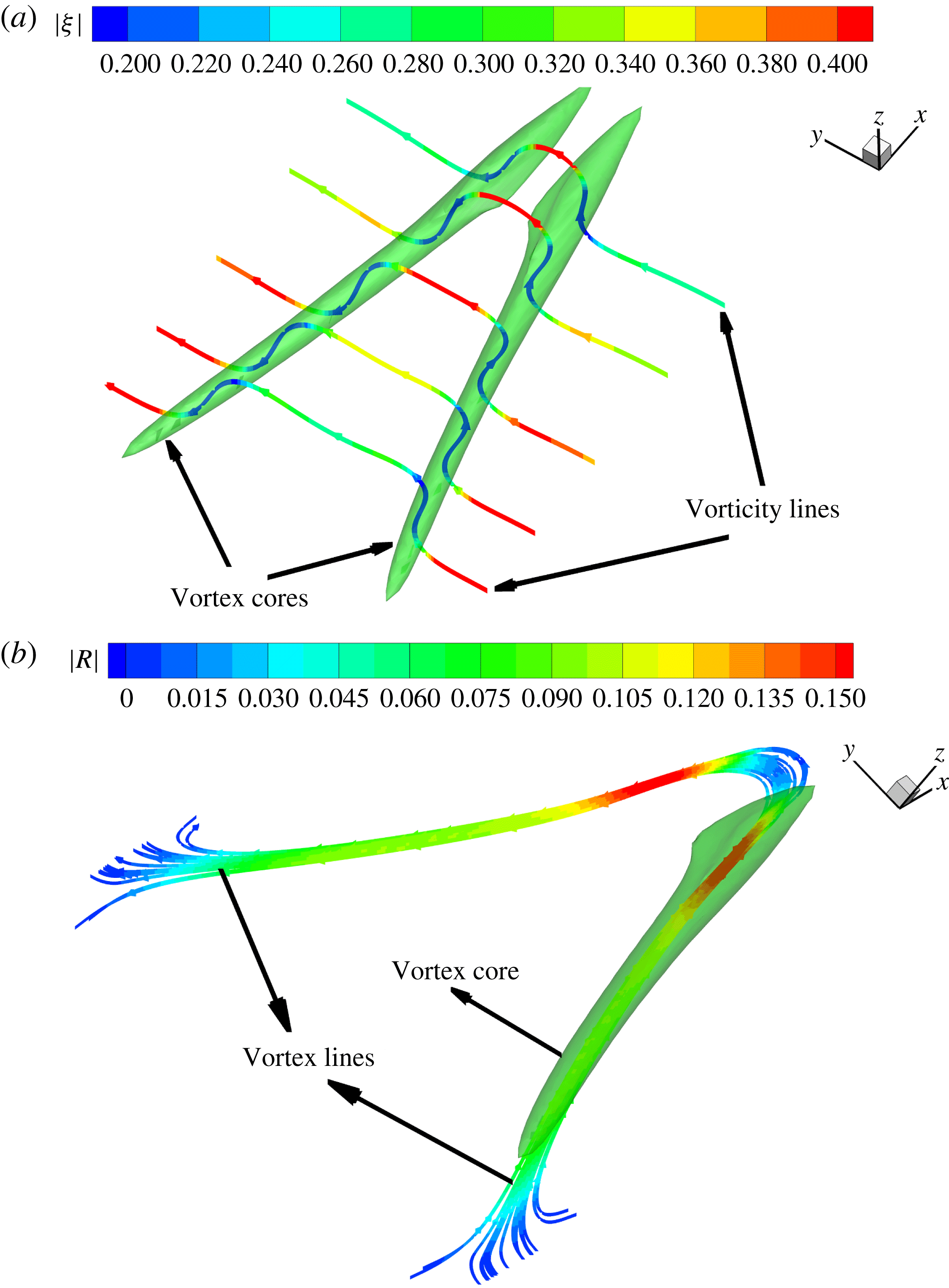
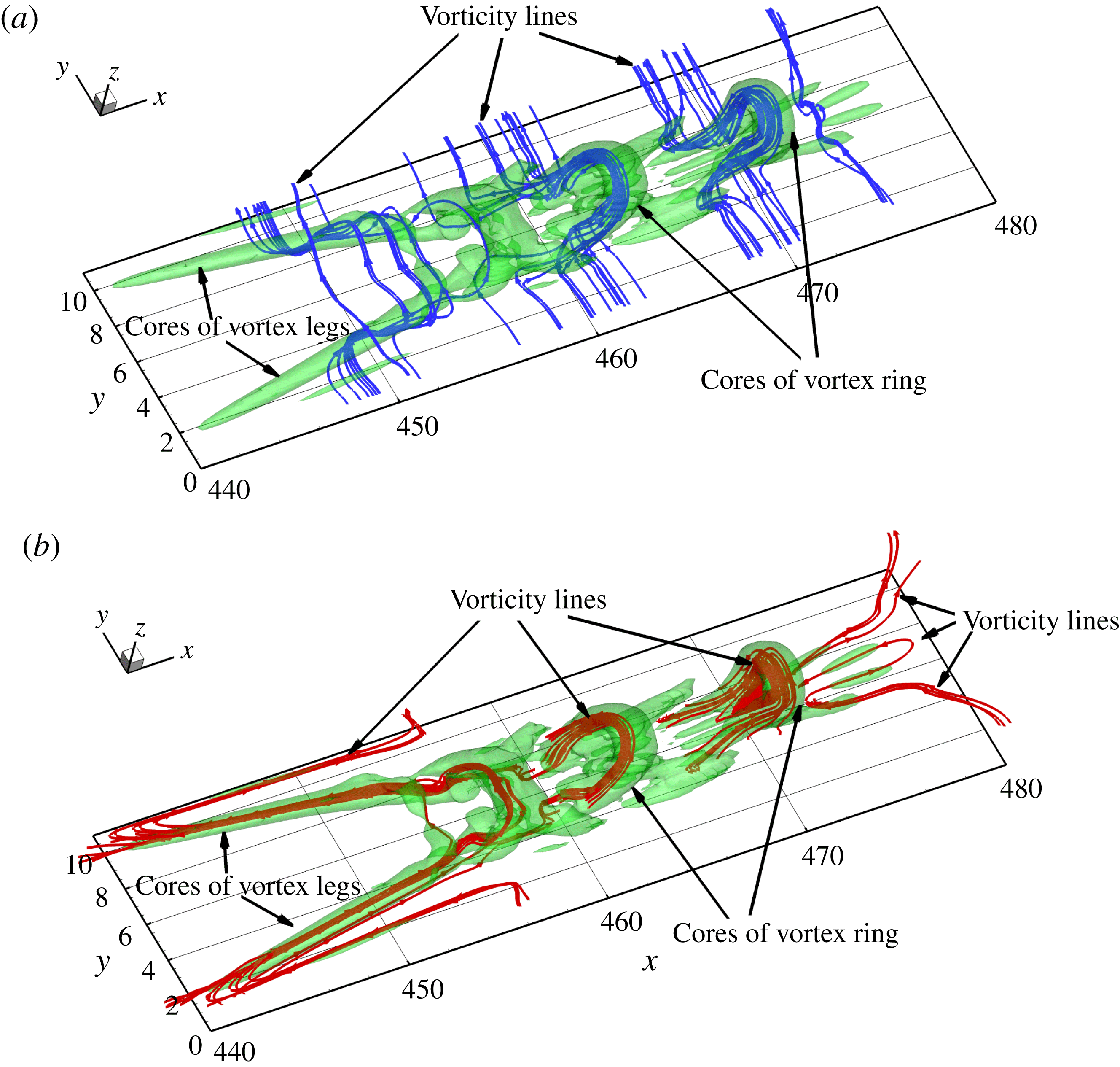
In classic vorticity dynamics, the vortices are always regarded as vorticity lines or tubes. However, they cannot fully describe the real vortex structures, even for a case as simple as a $\unicode[STIX]{x1D6EC}$ vortex. As shown in figure 8(a), the vorticity lines are created through points in the core of a $\unicode[STIX]{x1D6EC}$ vortex and it can be seen that the structure of the vorticity lines is totally different from that of the $\unicode[STIX]{x1D6EC}$ vortex. There are only a small portion of vorticity lines roughly aligned with the cores of vortex, but the new vortex lines defined in § 3 of this paper have the same structure as the cores of the $\unicode[STIX]{x1D6EC}$ vortex, see figure 8(b) in which the vortex lines are created inside the vortex core. These vortex lines are all aligned with the vortex core direction. In figure 8, the vorticity lines and vortex lines are coloured with the magnitude of the vorticity and vortex vector, respectively. It can be seen that as the rotational part of the vorticity, i.e. the vortex vector, cannot only fully describe the vortex structure but can also quantitatively give the strength of fluid rotation, where the red colour represents stronger rotation.

Figure 8.

Comparison of vorticity lines with vortex lines. (a) Vorticity lines which are created through points in the vortex core are not aligned with the cores of the $\unicode[STIX]{x1D6EC}$ vortex legs and cannot be used to represent the vortex. (b) Vortex lines which are also created through the points in the vortex cores are aligned with the cores of the $\unicode[STIX]{x1D6EC}$ vortex legs and can represent the structure of the vortex.

Figure 9.

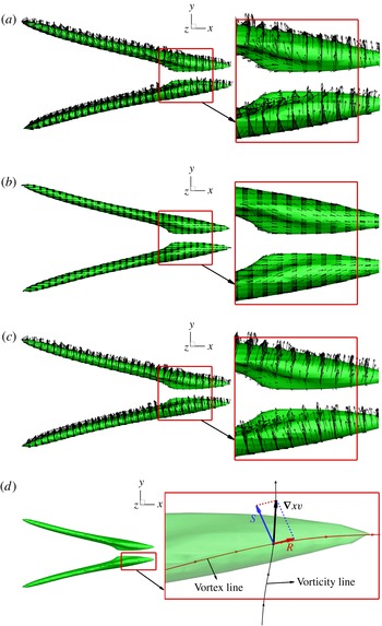
Compare the vector of vorticity with the vortex vector on the cores of the vortices which are illustrated by the iso-surface of $|\boldsymbol{R}|=0.075$ . (a) The vector of vorticity which is not aligned with (even orthogonal to) the vortex core and cannot fully describe the vortex. (b) The vector of the vortex vector which is aligned with the core of the $\unicode[STIX]{x1D6EC}$ vortex can represent the vortex. (c) The vector of shear vector which is the non-rotational part of the vorticity. (d) Comparison of the vectors of vorticity, vortex vector and shear vector at a point.

Different from vortex identification methods such as the $\unicode[STIX]{x1D6E5}$ -criterion, $Q$ -criterion, $\unicode[STIX]{x1D706}_{ci}$ -criterion, $\unicode[STIX]{x1D706}_{2}$ -criterion and $\unicode[STIX]{x1D6FA}$ -criterion, which are scalar quantities, the vortex vector, as a vector quantity, can also show the direction of local fluid rotation. In order to further compare the difference between the vorticity and vortex vector, the vectors on the vortex cores, which are illustrated by the iso-surface of $|\boldsymbol{R}|=0.075$ , are shown in figure 9. As we can see, the vector of vorticity is not aligned (even orthogonal to) with the vortex core (see figure 9 a), but the vortex vector is highly aligned with all parts of the $\unicode[STIX]{x1D6EC}$ vortex cores (see figure 9 b). The shear vector is also shown on the vortex cores and it has a very similar distribution as vorticity, see figures 9(a) and 9(c). When we draw the vectors of vorticity $\unicode[STIX]{x1D735}\times \boldsymbol{v}$ , the vortex vector $\boldsymbol{R}$ and shear vector $\boldsymbol{S}$ at the same point and create the vortex line and vorticity line through that point, it can be seen clearly that the vortex line and vortex vector are aligned with the vortex core, the vortex vector can represent fluid rotation and the vortex vector is the rotational part of the vorticity. However, the vector of vorticity has a different direction from the vortex and it further shows that vorticity cannot represent the rotation of the fluid. On the iso-surface of $|\boldsymbol{R}|=0.075$ , the shear vector is the main part of the vorticity at that point located at the tip of the $\unicode[STIX]{x1D6EC}$ vortex, as shown in figure 9(d). The vector distributions of the vortex vector and vorticity further imply that the vortex vector can fully describe the vortex structure, but the vorticity cannot for 3-D vortices. Actually, we have the formula: $\unicode[STIX]{x1D735}\times \boldsymbol{v}=\boldsymbol{R}+\boldsymbol{S}$ , which means the vorticity should be further decomposed into the vortex vector and shear vector.

In the process of late boundary layer transition, the hairpin vortex is a common vortex structure (Adrian Reference Adrian2007) and the flow structure is dominated by the hairpin vortices after the overshoot of skin friction (Sayadi, Hamman & Moin Reference Sayadi, Hamman and Moin2013). In natural flow transition, the hairpin vortices always appear in packets, as shown in figure 10 where a typical packet of hairpin vortices is visualized by using the iso-surface of $Q=0.02$ (see figure 10 a) and the magnitude of the vortex vector $|\boldsymbol{R}|=0.075$ (see figure 10 b). Similar to the example of a $\unicode[STIX]{x1D6EC}$ vortex, both methods give a similar structure for the vortices. However, the iso-surface of the vortex vector can show more small vortices while keeping the same shape and size of the large vortices than the $Q$ -criterion. This implies that the iso-surface of the magnitude of the vortex vector can correctly and accurately represent the topology and geometry of the vortex core structures of the complex vortices.

Figure 10.

Typical structure of a packet of hairpin vortices illustrated by (a) iso-surface of $Q=0.02$ ; (b) iso-surface of the magnitude of the vortex vector $|\boldsymbol{R}|=0.075$ .

Figure 11.

The distribution of vorticity lines and vortex lines. (a) Vorticity lines which are not consistent with the cores of vortices. (b) Vortex lines which are aligned to the cores of the complex vortices.

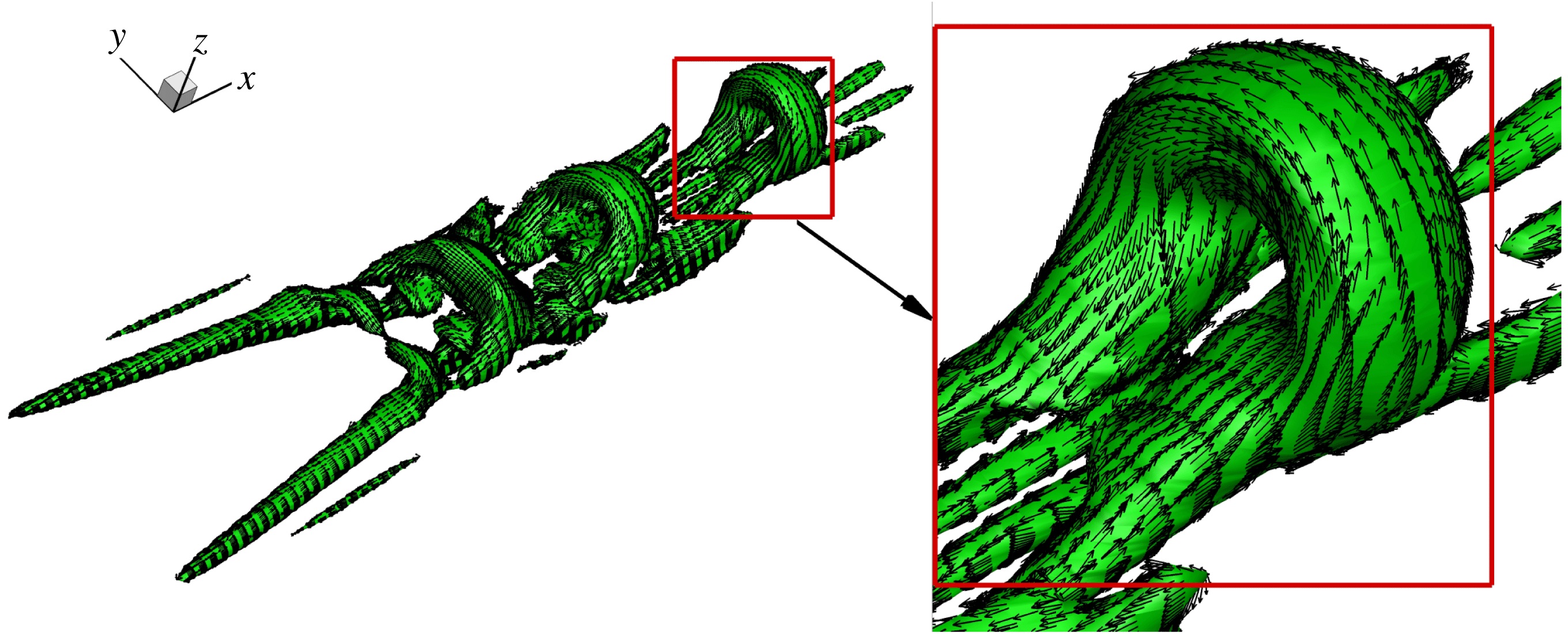
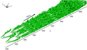
Figure 11 shows the structures of the vorticity lines and vortex lines which are all created through the same points. As can be seen, both vorticity lines and vortex lines can represent the topology of the ring of the hairpin vortex, but only the vortex lines are consistent with all vortex cores. The analysis of the distribution of vorticity and vortex vectors shows that the ring of the hairpin vortex is a very strong vortex core and a large part of the vorticity is rotational vorticity or the vortex vector. However, the other parts of the packet of the hairpin vortex are weak and the vortex vector is only a small part of the vorticity, so that the vorticity lines through those points in the weak vortex cores are not aligned to the vortex cores and only the vortex lines are always consistent with the vortex cores everywhere. This can be further verified by the vector distribution of the vortex vector (see figure 12) which illustrates vortex vectors on the surface of the core of the hairpin vortex packet. To show the ability of the vortex vector in describing the complex structure of the vortices, the vortical structures at one instant in the build-up of the laminar–turbulent flow transition process are visualized in figure 13 where the vortex cores are illustrated as the iso-surface of the magnitude of the vortex vector $|\boldsymbol{R}|=0.075$ . It can be found that the structures of the complex vortex can be correctly captured by the vortex vector. For these DNS data of the late flow transition, which contain a total of 60 million grid points, it only takes approximately 4.4 minutes to complete the calculation of the vortex vector on a regular laptop with a 2.9 GHz Intel Core i5 CPU and 8 GB memory.

Figure 12.

The distribution of vortex vectors on the vortex cores which are illustrated by the iso-surface of $|\boldsymbol{R}|=0.075$ .

Figure 13.

The process of vortical structure build-up in laminar–turbulent flow transition visualized by the iso-surface of the magnitude of the vortex vector $|\boldsymbol{R}|=0.075$ .

From the applications of the vorticity and vortex vector to describing the vortices in the late boundary layer transition, it can be found that the vorticity cannot fully describe the rotation of the fluid and the vorticity line or tube cannot well represent the vortex structure of the complex flow field. However, the newly defined vortex vector can fully represent the fluid rotation and can fully describe the vortices, even if they are as complex as vortices in turbulence. The vortex can be visualized by the vortex line, vortex tube or the iso-surface of the magnitude of the vortex vector. Different from the traditional vortex identification methods, the vortex vector cannot only visualize the structures of the vortex cores but also shows the rotation direction and the accurate strength of the vortex.

4.4 Vortical structures after micro-vortex generator (MVG)

For most vortex identification methods, there are problems when they are applied to compressible flow and modification is required (Kolář & Šístek Reference Kolář and Šístek2015; Epps Reference Epps2017). However, from the mathematical definition of our new vortex vector, it can be seen that the derivation is based on the analysis of the kinematics of a fluid element and it is not related to the compressibility of the flow. Therefore, the vortex vector only depends on the field of the velocity and therefore it can be used in any type of flow field. To show the ability in describing the complex vortical structures in compressible flow, a MVG (micro-vortex generator) case with an inflow $Ma=2.5$ is used as the last example in this paper. MVG is a passive control device aiming to alleviate flow separation. The previous study (Yang, Yan & Liu Reference Yang, Yan and Liu2016) shows that MVG can produce strong vortex rings and that the ring-like vortical structures could reduce the flow separation. The computational domain is the same as given by Yang et al. (Reference Yang, Yan and Liu2016) and the flow field is simulated by the LES method in which the fifth-order bandwidth-optimized weighted essentially non-oscillatory (WENO) scheme is used.

Figure 14.

The distribution of vorticity lines and vortex lines. (a) Vorticity lines which are not consistent with the cores of the vortices. (b) Vortex lines which are aligned to the cores of the complex vortices.

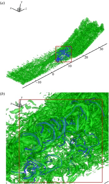
The complex vortical structures near the MVG are visualized by the iso-surface of the magnitude of the vortex vector $|\boldsymbol{R}|=1$ , see figure 14 in which the global view (figure 14 a) and local view (figure 14 b) of the vortical structures are presented. As we can see, the vortex vector defined in this paper can clearly capture the large ring-like vortex structures and the small vortices at the same time, even in such a complex case with interaction of the shock wave and turbulent boundary layers. The structures of the vortex lines (blue lines in figure 14 b) are also consistent with the cores of the vortices. This reveals that the newly defined vortex vector can well describe the vortical structures even in compressible turbulence.