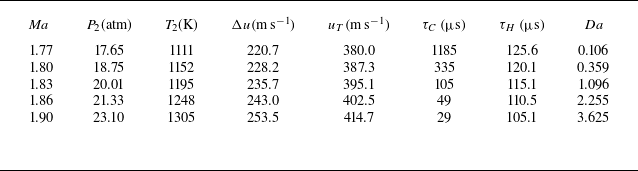
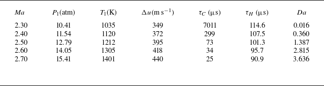
1. Introduction
Richtmyer–Meshkov instability (RMI) (Richtmyer Reference Richtmyer1960; Meshkov Reference Meshkov1969) occurs when a shock wave impulsively accelerates a perturbed interface between two fluids of different densities. Following shock impact, initial perturbations on the interface evolve through three distinct phases: initial linear growth, subsequent nonlinear growth and eventual transition to turbulent mixing. As a fundamental hydrodynamic instability, RMI plays a pivotal role in interface dynamics and mixing across a broad range of natural and industrial fields. For example, in inertial confinement fusion, laser-driven shock waves traverse material interfaces within the fuel capsule, initiating the RMI, which subsequently promotes mixing between the inner fuel and the outer ablator. This undesired mixing significantly degrades fusion energy yield and may even result in ignition failure (Lindl et al. Reference Lindl, Landen, Edwards, Moses and Team2014; Roycroft, Sauppe & Bradley Reference Roycroft, Sauppe and Bradley2022; Abu-Shawareb et al. Reference Abu-Shawareb, Acree, Adams, Adams, Addis, Aden, Adrian, Afeyan and Aggleton2024). In scramjets, achieving fast mixing between the fuel and oxidiser remains challenging due to extremely short residence times of reactants (Urzay Reference Urzay2018). As noted by Huete et al. (Reference Huete, Sánchez, Williams and Urzay2015), RMI has been increasingly recognised as an effective means to enhance fuel–oxidiser mixing and facilitate faster combustion.
Considering the interplay between interface dynamics and chemical reactions, RMI can be categorised into two fundamental types: inert RMI, where the material composition remains invariant and the interface evolution is purely hydrodynamic; and reactive RMI, where chemical reactions actively participate in the interface evolution. Extensive research on inert RMI has been conducted through theoretical (e.g. Zhang & Sohn Reference Zhang and Sohn1997; Wouchuk Reference Wouchuk2001; Mikaelian Reference Mikaelian2005; Dimonte & Ramaprabhu Reference Dimonte and Ramaprabhu2010; Zhang & Guo Reference Zhang and Guo2016; Zhang, Deng & Guo Reference Zhang, Deng and Guo2018), experimental (e.g. Sadot et al. Reference Sadot, Erez, Alon, Oron, Levin, Erez, Ben-Dor and Shvarts1998; Jacobs & Krivets Reference Jacobs and Krivets2005; Balakumar et al. Reference Balakumar, Orlicz, Tomkins and Prestridge2008; Morgan et al. Reference Morgan, Aure, Stockero, Greenough and Cabot2012; Mansoor et al. Reference Mansoor, Dalton, Martinez, Desjardins, Charonko and Prestridge2020; Wang et al. Reference Wang, Ding, Si and Luo2022; Noble et al. Reference Noble, Ames, McConnell, Oakley, Rothamer and Bonazza2023; Ferguson & Jacobs Reference Ferguson and Jacobs2024; Zhang et al. Reference Zhang, Zhao, Zhou, Ding and Luo2025a ) and numerical (e.g. Youngs & Williams Reference Youngs and Williams2008; Latini et al. Reference Latini, Schilling and Don2007b ; Zhou et al. Reference Zhou, Ding, Cheng and Luo2023a ; Sadler et al. Reference Sadler, Powell, Schalles, Louie, Jacobs and Zhou2024; Zhou et al. Reference Zhou, Ding and Cheng2024; Yan et al. Reference Yan, Chen, Li, Wu, Fan, Yu, Li and Wang2025; Zhang et al. Reference Zhang, Zhou, Cheng, Ding and Luo2025b ) approaches, with comprehensive reviews synthesising these findings (Zhou Reference Zhou2017a , Reference Zhoub ; Zhou, Sadler & Hurricane Reference Zhou, Sadler and Hurricane2025). However, reactive RMI has received much less attention, despite its broader practical significance in combustion and propulsion systems. This instability, involving complex interactions between hydrodynamic mechanisms and chemical kinetics, poses significant theoretical challenges (Bambauer, Hasslberger & Ozel-Erol Reference Bambauer, Hasslberger and Ozel-Erol2023; Napieralski et al. Reference Napieralski, Cobos, Sánchez-Sanz and Huete2024). Experimentally, it is equally difficult to study reactive RMI due to the challenges in reproducing the required high-temperature and high-pressure conditions. As a result, researchers have increasingly relied on numerical simulations as the primary tool for investigating reactive RMI (Fan et al. Reference Fan, Hao, Guan, Wen and Shi2022; Yan et al. Reference Yan, Fu, Wang, Yu and Li2022b ; Gong et al. Reference Gong, Zhao, Chen, Li, Zhou and Qiu2023; Napieralski et al. Reference Napieralski, Cobos, Sánchez-Sanz and Huete2024).
The reactive RMI can be further divided into non-premixed and premixed configurations. In premixed configurations, fuel and oxidiser are uniformly mixed before shock arrival, whereas in non-premixed configurations, they are initially separated by a distinct interface. In non-premixed systems, where a shock wave interacts with a fuel–oxidiser interface, the focus is on the dynamics of mixing and ignition (Zhou et al. Reference Zhou2021). For instance, Billet, Giovangigli & de Gassowski (Reference Billet, Giovangigli and de Gassowski2008) numerically investigated the interaction between a planar shock and a hydrogen bubble within an air atmosphere, revealing the significant influence of bulk viscosity on vorticity production and mixing. Similarly, Attal & Ramaprabhu (Reference Attal and Ramaprabhu2015) investigated the reactive RMI at a hydrogen/oxygen interface with varied thicknesses, demonstrating that combustion waves accelerate the perturbation growth. Recently, Yan et al. (Reference Yan, Fu, Wang, Yu and Li2022b ) performed three-dimensional (3-D) direct numerical simulations on cylindrical reactive RMI at a non-premixed hydrogen/oxygen interface with initial multimode perturbations. Their results indicated that chemical reactions promote mixing width growth through combustion waves, while simultaneously suppressing turbulent fluctuations due to increased heat release that causes greater viscous dissipation.
Premixed combustion has garnered more attention than non-premixed systems due to its higher combustion efficiency. Existing studies on reactive RMI involving premixed gases primarily fall into two areas: shock–flame interaction and shock–bubble interaction, where the bubble contains a premixed combustible gas within an inert atmosphere. In shock–flame interactions, a stable flame is first formed by igniting a homogeneous fuel–oxidiser mixture, across which the mixture transitions from dense, unburnt reactants to lighter burnt products. As a shock wave impinges upon the flame, RMI emerges, leading to significant changes in flame morphology. Both experiments (Markstein Reference Markstein1957; Thomas, Bambrey & Brown Reference Thomas, Bambrey and Brown2001) and numerical simulations (Khokhlov et al. Reference Khokhlov, Oran and Thomas1999b ; Ju, Shimano & Inoue Reference Ju, Shimano and Inoue1998; Jiang et al. Reference Jiang, Dong, Chen and Li2016a ; Bambauer et al. Reference Bambauer, Hasslberger and Ozel-Erol2023) have shown that RMI can significantly increase combustion rates via baroclinic vorticity that drives flame deformation, while combustion itself tends to suppress flame wrinkling by consuming small-scale vortices. Pioneering two-dimensional (2-D) simulations by Khokhlov et al. (Reference Khokhlov, Oran, Chtchelkanova and Wheeler1999a ) examined the interaction between a planar shock and a sinusoidally perturbed flame, revealing that reactive RMI can increase the energy yield rate by nearly 30-fold compared with non-reactive scenarios. Subsequent simulations by Bengoechea et al. (Reference Bengoechea, Stein, Reiss and Sesterhenn2015) highlighted an intriguing finding: combustion increases heat release while simultaneously stabilising RMI. A key theoretical contribution was made by Jiang et al. (Reference Jiang, Dong, Chen and Li2016a ), who introduced a dimensionless parameter from the ratio of two characteristic time scales: the chemical reaction time scale and the RMI time scale. Their analysis demonstrated that this time scale ratio fundamentally determines the evolution of reactive RMI. In subsequent work, Jiang et al. (Reference Jiang, Dong, Chen and Wu2016b ) and Chen, Dong & Jiang (Reference Chen, Dong and Jiang2017) examined perturbation growth on 3-D flames under multiple shock impacts, observing significantly enhanced growth rates.
A reactive shock–bubble interaction, where a shock wave interacts with a spherical bubble containing premixed fuel and oxidiser, is a fundamental case for studying reactive RMI. This interaction not only triggers RMI on the bubble surface but also induces ignition through the shock-focusing mechanism. The pioneering experimental study on reactive shock–bubble interaction, reported by Haehn et al. (Reference Haehn, Ranjan, Weber, Oakley, Rothamer and Bonazza2012), introduced the concept of dual Mach number limits: a lower limit controlling ignition occurrence and an upper limit marking the onset of detonation. Subsequently, Diegelmann et al. (Reference Diegelmann, Hickel and Adams2016a , Reference Diegelmann, Tritschler, Hickel and Adamsb ) investigated the upper Mach limit via 2-D numerical simulations, highlighting the significant influence of reaction wave types on bubble evolution. This research was later extended to 3-D simulations using quarter-bubble configurations (Diegelmann, Hickel & Adams Reference Diegelmann, Hickel and Adams2017). More recently, Fan et al. (Reference Fan, Hao, Guan, Wen and Shi2022) investigated deflagration combustion in spherical bubbles, focusing on the lower Mach number limit. Their results revealed that the thermal effects of combustion enhance mixing efficiency by approximately 150 %. Despite these advances, the shock–bubble interaction represents only one specific case of reactive RMI, and the spherical geometry poses challenges for the quantitative analysis of RMI effects. In contrast, the single-mode interface provides a more fundamental configuration for studying RMI, as arbitrary multimode perturbations can be decomposed into a superposition of single-mode perturbations via Fourier transform. This foundational role is further reflected in the fact that most classical RMI theories, including linear and nonlinear growth models (Wouchuk Reference Wouchuk2001; Mikaelian Reference Mikaelian2005; Dimonte & Ramaprabhu Reference Dimonte and Ramaprabhu2010; Zhang et al. Reference Zhang, Deng and Guo2018), were developed based on single-mode interfaces. This fundamental nature makes it an ideal configuration for investigating the essential physics of reactive RMI, which motivates the present study.
In this work a compressible, reactive, multicomponent Navier–Stokes solver is first developed and extensively validated through a series of benchmark tests. Using this high-order solver, a comprehensive numerical study of reactive RMI at a single-mode interface separating inert and premixed gases under various incident shock Mach numbers is then conducted. Four distinct evolution regimes, characterised by different coupling intensities between interface development and combustion processes, are identified. By quantitatively analysing the evolution of key quantities including the mixing width, mixing level and enstrophy, the influence of combustion on interface dynamics is revealed within each regime. Analyses on vorticity transport mechanisms and characteristic time scales show how the relative dominance between hydrodynamic and reactive effects varies across different regimes. The findings will show that the coupling intensity between flow and combustion does not monotonically increase with reaction rate, but rather depends on the matching of their characteristic time scales.
2. Numerical methods
2.1. Governing equations
The 2-D compressible multicomponent Navier–Stokes equations are employed to characterise reactive RMI involving
 $ns$
species. In Cartesian coordinates, the governing equations take the following conservative form:
 \begin{equation} \dfrac {\partial \boldsymbol{U}}{\partial t} + \dfrac {\partial (\boldsymbol{F} - \boldsymbol{F_v})}{\partial x} + \dfrac {\partial (\boldsymbol{G} - \boldsymbol{G_v})}{\partial y} = \boldsymbol{S_c}. \end{equation}
Here
 $\boldsymbol{U}$
denotes the vector of conservative variables,
 $\boldsymbol{F}$
and
 $\boldsymbol{G}$
are the inviscid flux vectors, and
 $\boldsymbol{F_v}$
and
 $\boldsymbol{G_v}$
are the viscous flux vectors in the
 $x$
and
 $y$
directions, respectively. Their explicit forms are provided as follows:
 \begin{align} \boldsymbol{U} &= [\rho _1 , {\cdots} ,\rho _{\textit{ns}} ,\rho u ,\rho v ,\rho E ]^T , \end{align}
 \begin{align} \boldsymbol{F} &= [\rho _1 u , {\cdots} ,\rho _{\textit{ns}} u ,\rho u^2+p,\rho u v,(\rho E + p) u ]^T, \end{align}
 \begin{align} \boldsymbol{G} &= [\rho _1 v , {\cdots} ,\rho _{\textit{ns}} v ,\rho u v,\rho v^2+p,(\rho E + p) v ]^T, \end{align}
 \begin{align} \boldsymbol{F_v} &= [-J_{1,x} , {\cdots} ,-J_{ns,x} ,\tau _{\textit{xx}} ,\tau _{\textit{xy}} ,u \tau _{\textit{xx}} + v \tau _{\textit{xy}} - q_{\textit{cx}} -q_{\textit{dx}} ]^T , \end{align}
 \begin{align} \boldsymbol{G_v} &= [-J_{1,y} , {\cdots} ,-J_{ns,y} ,\tau _{\textit{xy}} ,\tau _{\textit{yy}} ,u \tau _{\textit{xy}} + v \tau _{\textit{yy}} - q_{cy} -q_{\textit{dy}} ]^T . \end{align}
The source term
 $S_c$
arising from chemical reactions is given by
 \begin{equation} \boldsymbol{S_c} = [\dot {\omega }_1, {\cdots} , \dot {\omega }_{\textit{ns}}, 0, 0, 0]^T, \end{equation}
where
 $\rho _i$
denotes the density of species
 $i$
,
 $\rho$
is the total mixture density,
 $u$
and
 $v$
represent the velocity components and
 $p$
is the static pressure. Additionally,
 $J_{i,j}$
is the mass diffusion flux,
 $\tau _{\textit{ij}}$
denotes viscous stress components,
 $q_{ci}$
is the conductive heat flux and
 $q_{di}$
is the interspecies enthalpy flux. The term
 $\dot {\omega }_i$
denotes the mass production rate of the
 $i$
th species due to chemical reactions. The mass diffusion flux
 $J_{i,j}$
is modelled based on Fick’s law, with an additional correction term to enforce mass conservation:
 \begin{align} J_{i,x} &= -\rho \left (D_i \dfrac {\partial Y_i}{\partial x} - Y_i \sum _{m=1}^{\textit{ns}} D_m \dfrac {\partial Y_m}{\partial x}\right )\!, \end{align}
 \begin{align} J_{i,y} &= -\rho \left (D_i \dfrac {\partial Y_i}{\partial y} - Y_i \sum _{m=1}^{\textit{ns}} D_m \dfrac {\partial Y_m}{\partial y}\right )\!. \end{align}
Here,
 $D_i$
represents the mixture-averaged diffusion coefficient of the
 $i$
th species, which is computed from binary diffusion coefficients
 $D_{\textit{ij}}$
as
 \begin{equation} D_i = \dfrac {1-X_i}{\sum _{j \neq i}^{\textit{ns}} X_j/D_{\textit{ij}}}, \end{equation}
with
 $X_i$
and
 $Y_i$
being the mole and mass fractions, respectively. Under Stokes’ hypothesis and also neglecting bulk viscosity, the components of the viscous stress tensor are
 \begin{align} \tau _{\textit{xx}} &= \dfrac {2\mu }{3} \left (2\dfrac {\partial u}{\partial x}-\dfrac {\partial v}{\partial y}\right )\!, \end{align}
 \begin{align} \tau _{\textit{yy}} &= \dfrac {2\mu }{3} \left (2\dfrac {\partial v}{\partial y}-\dfrac {\partial u}{\partial x}\right )\!, \end{align}
 \begin{align} \tau _{\textit{xy}} &= \tau _{\textit{yx}} = \mu \left (\dfrac {\partial u}{\partial y}+\dfrac {\partial v}{\partial x}\right )\!, \end{align}
where
 $\mu$
is viscosity coefficient of the mixture. The total heat flux in the system comprises two primary contributions: conductive heat flux, which follows Fourier’s law, and interspecies enthalpy diffusion. These components are mathematically expressed as
 \begin{align} q_{\textit{cx}} &= -\kappa \dfrac {\partial T}{\partial x}, \quad q_{cy} = -\kappa \dfrac {\partial T}{\partial y}, \end{align}
 \begin{align} q_{\textit{dx}} &= \sum _{i=1}^{\textit{ns}} h_i J_{i,x}, \quad q_{\textit{dy}} = \sum _{i=1}^{\textit{ns}} h_i J_{i,y}, \end{align}
where
 $\kappa$
represents the thermal conductivity of the mixture and
 $h_i$
is the specific enthalpy of species
 $i$
. The mixture transport properties,
 $\mu$
and
 $\kappa$
, are evaluated using Wilke’s mixing rule:
 \begin{align} \mu &= \sum _{i=1}^{\textit{ns}} \dfrac {X_i}{\phi _i} \mu _i, \end{align}
 \begin{align} \kappa &= \sum _{i=1}^{\textit{ns}} \dfrac {X_i}{\phi _i} \kappa _i, \end{align}
 \begin{align} \phi _i &= \sum _{m=1}^{\textit{ns}} \dfrac {X_m\left \{1+\sqrt {\dfrac {\mu _i}{\mu _m}}\left (\dfrac {M_m}{M_i}\right )^{\tfrac {1}{4}} \right \}^2}{\sqrt {8\left (1+\dfrac {M_i}{M_m}\right )}}. \end{align}
Here
 $\mu _i$
and
 $\kappa _i$
denote the viscosity and thermal conductivity of the
 $i$
th species in the mixture, respectively, while
 $M_i$
represents its molar mass. The species transport properties are evaluated based on Chapman–Enskog theory, Eucken’s relation and empirical constitutive laws, as detailed in Kee et al. (Reference Kee, Coltrin, Glarborg and Zhu2017).
2.2. Equations of state
The system of equations is closed by the equation of state for equilibrium thermodynamics, which is given by
 \begin{equation} E = \dfrac {1}{2} \rho (u^2 + v^2) + \sum _{i=1}^{\textit{ns}}\rho _i h_i - p, \end{equation}
where
 $E$
is the total energy per unit volume. The static pressure
 $p$
is determined according to Dalton’s law, i.e.
 \begin{equation} p = \sum _{i=1}^{\textit{ns}} p_i = \sum _{i=1}^{\textit{ns}} \rho _i R_i T, \end{equation}
where
 $R_i = R_u / M_i$
represents the specific gas constant for the
 $i$
th species. Here,
 $R_u=8.314\,\mathrm{ J\,mol^{-1} K^{-1}}$
is the universal gas constant. According to Gordon (Reference Gordon1976), the thermodynamic properties are calculated using polynomial fits as
 \begin{align} \dfrac {C_{\!p,i}}{R_i} &= A_i + B_i T + C_i T^2 + D_i T^3 + E_i T^4, \end{align}
 \begin{align} \dfrac {h_i}{R_i} &= A_i T + \dfrac {1}{2} B_i T^2 + \dfrac {1}{3} C_i T^3 + \dfrac {1}{4} D_i T^4 + \dfrac {1}{5} E_i T^5 + F_i, \end{align}
 \begin{align} \dfrac {S_i}{R_i} &= A_i \ln T + B_i T + \dfrac {1}{2} C_i T^2 + \dfrac {1}{3} D_i T^3 + \dfrac {1}{4} E_i T^4 + G_i, \end{align}
where
 $A_i$
,
 $B_i$
,
 $C_i$
,
 $D_i$
,
 $E_i$
,
 $F_i$
and
 $G_i$
are species-specific curve-fit coefficients. These coefficients determine the specific heat at constant pressure (
 $C_{p,i}$
), enthalpy (
 $h_i$
) and entropy (
 $S_i$
) of species
 $i$
per unit mass. The mixture-averaged specific heat at constant pressure,
 $C_{\!p}$
, and the mixture-averaged enthalpy per unit mass,
 $h$
, are calculated using mass-fraction weighting as follows:
 \begin{align} C_{\!p} &= \sum _{i=1}^{\textit{ns}} Y_i C_{p,i}, \end{align}
 \begin{align} h &= \sum _{i=1}^{\textit{ns}} Y_i h_i. \end{align}
2.3. Chemical reaction kinetics
For a system consisting of
 $nr$
elementary reactions among
 $ns$
species, the general chemical kinetic model is expressed as
 \begin{equation} \sum _{i=1}^{\textit{ns}} a_{\textit{ij}} \chi _i \rightleftharpoons \sum _{i=1}^{\textit{ns}} b_{\textit{ij}} \chi _i, \quad j=1,2,\boldsymbol{\ldots} ,nr, \end{equation}
where
 $\chi _i$
denotes the
 $i$
th species, and
 $a_{\textit{ij}}$
and
 $b_{\textit{ij}}$
represent the stoichiometric coefficients of reactants and products, respectively, in the
 $j$
th reaction. The net mass production rate of species
 $i$
is calculated as
 \begin{equation} \dot {\omega }_i =\sum _{j=1}^{nr} M_i (\dfrac {{\rm d}[\chi _i]}{{\rm d}t})_j = \sum _{j=1}^{nr} M_i (b_{\textit{ij}}-a_{\textit{ij}}) (\eta _{f,j}-\eta _{b,j}), \end{equation}
where
 $[\chi _i]$
denotes the molar concentration of the
 $i$
th species, and
 $\eta _{f,j}$
and
 $\eta _{b,j}$
represent the forward and backward reaction rates of the
 $j$
th elementary reaction, respectively. These are expressed as follows:
 \begin{align} \eta _{f,j}&=k_{f,r}\prod _{i=1}^{\textit{ns}}[\chi _i]^{a_{\textit{ij}}}, \end{align}
 \begin{align} \eta _{b,j}&=k_{b,r}\prod _{i=1}^{\textit{ns}}[\chi _i]^{b_{\textit{ij}}}. \end{align}
Here,
 $k_{f,j}$
and
 $k_{b,j}$
denote the forward and backward reaction rate coefficients of the
 $j$
th reaction, respectively. For the H
 $_2$
/O
 $_2$
combustion system, the well-validated Kéromnès mechanism (Kéromnès et al. Reference Kéromnès2013) is employed, which comprises 10 species and 21 elementary reactions. The forward reaction rate coefficient is characterised by the Arrhenius expression
 \begin{equation} k_{f,j} = A_{f,j} T^{B_{f,j}} \exp \left (-\frac {E_{f,j}}{R_u T}\right )\!, \end{equation}
where
 $A_{f,j}$
,
 $B_{f,j}$
and
 $E_{f,j}$
are specific parameters for each reaction, as specified in the Kéromnès mechanism. The backward rate coefficient is determined by the equilibrium constant,
 $K_{c,j}$
, as
 \begin{align} k_{b,j} &= \frac {k_{f,j}}{K_{c,j}}, \end{align}
 \begin{align} K_{c,j} &= \exp \left [-\frac {\Delta G_j}{R_u T}+\ln \left (\frac {P_0}{R_u T}\right ) \sum _{i=1}^{\textit{ns}}(b_{\textit{ij}}-a_{\textit{ij}}) \right ]\!, \end{align}
where
 $P_0=101\,325$
Pa is the standard atmospheric pressure. The Gibbs free energy change,
 $\Delta G_j$
, for the
 $j$
th reaction is computed as
 \begin{equation} \Delta G_j=\sum _{i=1}^{\textit{ns}} M_i (h_i - T S_i) (b_{\textit{ij}}-a_{\textit{ij}}). \end{equation}
The Kéromnès mechanism also incorporates pressure-dependent fall-off reactions, which are modelled using the Troe formalism (Gilbert, Luther & Troe Reference Gilbert, Luther and Troe1983). Following Diegelmann et al. (Reference Diegelmann, Hickel and Adams2016a ), Xe and Ar are assumed to have equal third-body collision efficiencies due to their similar collisional properties. This assumption is particularly relevant to the present RMI simulations, where Xe is employed as the primary diluent.
2.4. Numerical schemes
The governing equations (2.1) exhibit strong stiffness, primarily arising from the chemical source term
 $\boldsymbol{S_c}$
. To address this stiffness, we employ an operator-splitting approach based on the second-order Strang splitting scheme. This approach decomposes the governing equations into two distinct subsets: a set of partial differential equations (PDEs) given by (2.34), which describe the fluid dynamics; and a set of ordinary differential equations (ODEs) given by (2.35), which characterise the chemical reactions. They are expressed as follows:
 \begin{align} \dfrac {\partial \boldsymbol{U}^*}{\partial t} &+ \dfrac {\partial (\boldsymbol{F} - \boldsymbol{F_v})}{\partial x} + \dfrac {\partial (\boldsymbol{G} - \boldsymbol{G_v})}{\partial y} = 0, \end{align}
 \begin{align} &\qquad\dfrac {\partial \boldsymbol{U}}{\partial t}= \dfrac {\partial \boldsymbol{U}^*}{\partial t} + \boldsymbol{S_c}. \end{align}
The numerical solution is advanced sequentially in three steps over each time interval
 $[t^n, t^n + \Delta t]$
as follows.
-
(i) Step 1 solves the fluid dynamics PDEs (2.34) over a half-time step, advancing the solution to obtain
 $U^*$
at
$t+\Delta t/2$
under the assumption of chemically frozen flow.
-
(ii) Step 2 integrates the chemical kinetics ODEs (2.35) over the full time interval
$\Delta t$
, using the updated
$U^*$
from part (i) as the initial condition. This yields the updated solution
$U$
at
$t+\Delta t$
, with chemical source terms accounted for. -
(iii) Step 3 completes the time advancement by solving the fluid dynamics PDEs (2.34) again for the remaining half-time step
$\Delta t/2$
. In this step, the updated conservative variables
$U$
from part (ii) are used as the initial condition, advancing the solution to the final state at
$t+\Delta t$
.


For further details on the time-advancement procedure of (2.34) and (2.35), readers are referred to Diegelmann et al. (Reference Diegelmann, Tritschler, Hickel and Adams2016b ). The chemical kinetics ODEs are solved using the DVODE solver (Jackson & Sacks-Davis Reference Jackson and Sacks-Davis1980; Brown, Byrne & Hindmarsh Reference Brown, Byrne and Hindmarsh1989), which features an adaptive time-stepping scheme based on the backward differentiation formula method. This solver efficiently addresses chemical stiffness, providing high accuracy through automatic step-size control and adaptive order selection. To solve the fluid dynamics equations, an in-house finite-difference code, initially developed for inert RMI, is extended in this work to simulate multicomponent reactive flows. A fifth-order weighted essentially non-oscillatory scheme combined with a double-flux algorithm is employed for spatial discretisation, which has demonstrated both accuracy and computational efficiency in resolving shock waves and material interfaces in our inert RMI studies (Ding et al. Reference Ding, Si, Yang, Lu, Zhai and Luo2017; Feng et al. Reference Feng, Xu, Zhai and Luo2021). In this work, to account for temperature-dependent thermodynamic properties, we incorporate a modified double-flux formulation following the approach of Billet & Abgrall (Reference Billet and Abgrall2003), ensuring consistency with polynomial expressions of specific heats, enthalpies and entropies. This hybrid numerical strategy combines the computational efficiency of operator splitting with the robustness of high-order shock-capturing schemes, thereby enabling accurate simulation of the complex interactions among shock waves, material interfaces and chemical reactions.
3. Numerical method validations
In this section we validate our numerical methods developed for reactive flows using three benchmark cases, progressing from zero-dimensional (0-D) to 2-D configurations. The 0-D ignition delay prediction is first performed without flow coupling to assess the accuracy of different chemical reaction mechanisms. The subsequent validation cases in §§ 3.2 and 3.3 progressively verify the correct implementation of the reaction mechanism coupled with fluid dynamics, advancing from 1-D laminar flames to 2-D reactive shock–bubble interactions. These cases comprehensively validate the integrated treatment of chemistry, molecular transport and hydrodynamics in our code.
3.1. The 0-D ignition delay time
In hydrogen–oxygen combustion, initial heating and subsequent chain reactions facilitate the accumulation of radicals as the premixed gas is heated. Once a sufficient concentration of radicals is reached, chain-termination reactions predominate, leading to the release of significant chemical energy into the flow, which is identified as ignition (Turns et al. Reference Turns1996). The interval between the onset of heating and ignition is defined as the ignition delay time. Accurate prediction of ignition delay time is crucial for effectively modelling premixed combustion, particularly under high-pressure and high-temperature conditions. Hence, we first evaluate ignition delay predictions for a stoichiometric H
 $_2$
/O
 $_2$
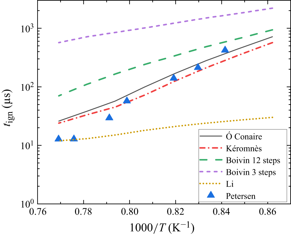
/Ar mixture (2 : 1 : 97 by volume) at a pressure of 33 atm, across a temperature range from 1160 K to 1310 K. Here, the ODEs corresponding to various chemical mechanisms, without flow coupling, are solved using the DVODE solver developed by Brown et al. (Reference Brown, Byrne and Hindmarsh1989). Figure 1 presents a comparison between ignition delay predictions from DVODE simulations employing various chemical mechanisms and experimental shock-tube data reported by Petersen et al. (Reference Petersen, Davidson, Röhrig and Hanson1995). The results indicate that the Kéromnès mechanism exhibits the closest agreement with experimental data under the high-pressure and high-temperature conditions. This confirms both the accuracy of the Kéromnès mechanism and the reliable implementation of the DVODE solver.
Comparison of ignition delay times for a stoichiometric H
 $_2$
/O
 $_2$
/Ar mixture (2 : 1 : 97 by volume) at 33 atm over the temperature range 1160–1310 K. Lines represent numerical predictions using various reaction mechanisms:
 $\acute {\text{O}}$
Conaire (Ó Conaire et al. Reference Conaire, Curran, H., Simmie, Pitz and Westbrook2004), Kéromnès (Kéromnès et al. Reference Kéromnès2013), Boivin (12 step and 3 step) (Boivin et al. Reference Boivin, Jiménez, Sánchez and Williams2011 and Li et al. Reference Li, Zhao, Kazakov and Dryer2004). Symbols denote experimental data from Petersen et al. (Reference Petersen, Davidson, Röhrig and Hanson1995).

The deviation of the Kéromnès model from experimental data at low
 $x$
-axis values, corresponding to the high-temperature region, can be attributed to three factors. First, at high temperatures, the ignition delay time becomes very short, making the measurements highly sensitive to small fluctuations in pressure and temperature within the shock tube. Second, uncertainties in temperature determination in shock-tube experiments can lead to significant errors in the measured ignition delay time (Petersen et al. Reference Petersen, Davidson, Röhrig and Hanson1995). Third, Petersen’s experiments employed OH laser diagnostics to measure the OH profile, and uncertainties in identifying the steepest slope of the OH signal may introduce additional measurement errors of up to approximately 5 % (Kéromnès et al. Reference Kéromnès2013).
3.2. The 1-D laminar flame
To validate the integrated treatment of molecular transport and chemical reactions, a 1-D laminar flame is simulated, following the methodology of Chung et al. (Reference Chung, Zhang, Kaplan and Oran2020). The simulation considers a stoichiometric hydrogen-air mixture under initial conditions of
 $p_0 = 17.24$
kPa and
 $T_0 = 294$
K. Two key flame characteristics are examined: the laminar burning velocity
 $S_l$
and the flame thickness
 $\delta _l$
. The laminar burning velocity in the flame reference frame is calculated as
 \begin{equation} S_l=\dfrac {\rho _b u_b - \rho _u u_u}{\rho _b - \rho _u} - u_u, \end{equation}
where
 $\rho _b$
and
 $\rho _u$
are the densities, and
 $u_b$
and
 $u_u$
are the velocities of the burnt and unburnt gases, respectively. The flame thickness is defined as the ratio of the temperature difference across the flame to the maximum temperature gradient, i.e.
 \begin{equation} \delta _l=\dfrac {(T_b-T_u)}{{|\partial T / \partial x|}_{\textrm{max}}}, \end{equation}
where
 $T_b$
and
 $T_u$
denote the temperatures of the burnt and unburnt gases, respectively, and
 ${|\partial T / \partial x|}_{\textrm{max}}$
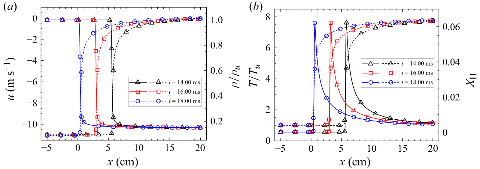
represents the maximum temperature gradient across the flame. Figure 2 presents the spatial distributions of temperature, velocity, density and H radical concentration within the flame. For all variables, the computed profiles exhibit steep gradients across the flame front while remaining free from spurious oscillations, highlighting the stability and resolution capability of the developed numerical method. With these data, the laminar burning velocity and flame thickness are calculated to be
 $S_l = 2.03$
 $\text{m s}^{-1}$
and
 $\delta _l = 0.35$
cm, respectively. Both parameters show good agreement with the results reported by Yang & Radulescu (Reference Yang and Radulescu2021), where
 $S_l = 1.98\,\text{m s}^{-1}$
and
 $\delta _l = 0.34\,\mathrm{cm}$
, and those of Xiao et al. (Reference Xiao, Shen, Si and Luo2024), where
 $S_l = 1.98\,\text{m s}^{-1}$
and
 $\delta _l = 0.375\,\mathrm{cm}$
, with relative errors below
 $5\%$
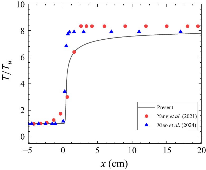
. To explain the slight deviations, we further compare the temperature fields from our simulations with those of Yang & Radulescu (Reference Yang and Radulescu2021) and Xiao et al. (Reference Xiao, Shen, Si and Luo2024), as shown in figure 3. The minor discrepancies arise because these previous studies employed a simplified one-step reaction mechanism, whereas the present work uses a detailed mechanism, resulting in small differences in scalar fields (such as temperature and pressure) and consequently in derived quantities such as burning velocity and flame thickness.
Spatial distributions of key parameters across a 1-D laminar flame at representative times. Panel (a) shows velocity (dotted lines) and density (solid lines) profiles, while panel (b) shows temperature (dotted lines) and H radical mass fraction (solid lines) profiles. Density and temperature are normalised by their respective unburnt values ahead of the flame front.

Spatial distributions of temperature across 1-D laminar flame. The symbols represent the results from Yang & Radulescu (Reference Yang and Radulescu2021) and Xiao et al. (Reference Xiao, Shen, Si and Luo2024), while the line represents the results from the present work.

3.3. The 2-D cylindrical reactive shock–bubble interaction
To further validate the integrated treatment of reactive kinetics and interfacial dynamics, numerical simulations of 2-D reactive shock–bubble interaction at two representative Mach numbers (
 ${\textit{Ma}}_1=2.30$
and
 ${\textit{Ma}}_2=2.90$
) are conducted. This test case closely follows the configuration proposed by Diegelmann et al. (Reference Diegelmann, Hickel and Adams2016a
), in which a shock wave interacts with a bubble containing a stoichiometric H
 $_2$
/O
 $_2$
mixture diluted with Xe, initially embedded in ambient air. To enable direct comparison with the results of Diegelmann et al. (Reference Diegelmann, Hickel and Adams2016a
), the present simulation employs a comparable grid resolution of
 $\Delta x=50$
 $\unicode {x03BC}\text{m}$
.
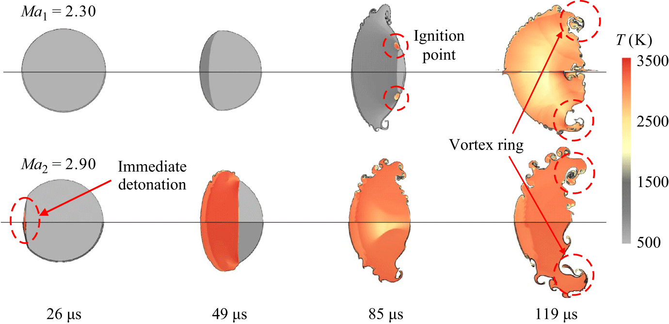
Figure 4 presents a comparison of the temperature fields obtained in the present simulation with those reported by Diegelmann et al. (Reference Diegelmann, Hickel and Adams2016a
). The bubble interface is visualised using isocontours of the Xe mass fraction (
 $Y_{\text{Xe}}$
) ranging from 0.35 to 0.55, following the methodology of Fan et al. (Reference Fan, Hao, Guan, Wen and Shi2022). In the
 ${\textit{Ma}} = 2.30$
case, our simulation accurately captures both the ignition timing (
 $85\ \unicode {x03BC}\text{s}$
) and the ignition location, which occurs near the upper surface of the bubble. In the higher-Mach-number case (
 ${\textit{Ma}} = 2.90$
), the simulation successfully reproduces the prompt detonation initiation occurring
 $26\ \unicode {x03BC}\text{s}$
after shock impact. The close agreement in key flow features, including vortex dynamics, temperature distribution and the evolution of the reaction front, across both cases highlights the reliability and robustness of the proposed numerical framework in simulating reactive RMI.
Temperature contours for reactive shock–bubble interactions at
 ${\textit{Ma}} = 2.30$
and
 ${\textit{Ma}} = 2.90$
. Each subfigure compares the results of Diegelmann et al. (Reference Diegelmann, Hickel and Adams2016a
) (above the symmetry axis) with the present simulations (below). The black lines indicate the bubble interface, defined by the isocontour
 $Y_{\text{Xe}} = 0.35$
.

4. Simulation of reactive RMI at single-mode interfaces
4.1. Computational set-up
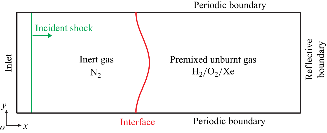
As illustrated in figure 5, we employ a 2-D rectangular computational domain with dimensions
 $5L_0 \times L_0$
(
 $L_0 = 40\,\mathrm{mm}$
), which is discretised by a Cartesian mesh of
 $2000 \times 400$
cells, corresponding to a grid spacing of
 $\Delta x = \Delta y = 100\,\unicode {x03BC}\mathrm{m}$
. Boundary conditions are specified as follows: an inlet boundary at the left side, a reflective, adiabatic boundary at the right side and periodic boundaries at both the upper and lower sides. Initially, a sinusoidal interface is positioned at
 $x=0.5L_0$
, separating two distinct gas regions: pure N
 $_2$
on the left and a premixed gas mixture of H
 $_2$
/O
 $_2$
/Xe (2:1:97 by volume) on the right. The sinusoidal interface features a fixed wavelength
 $\lambda _0=40\;\text{mm}$
and an initial perturbation amplitude
 $a_0=2\;\text{mm}$
.
Schematic of the computational set-up.

An incident shock wave is initialised at
 $x=0.25L_0$
and propagates rightward. The pre-shock gas is at atmospheric temperature and pressure (
 $T_0=298\;\text{K}$
,
 $P_0=101\,325\;\text{Pa}$
), and its velocity relative to the incident shock wave is
 $V_0 = -a_{N_2} \boldsymbol{\cdot }Ma$
, where
 $a_{N_2}$
is the speed of sound in nitrogen. The post-shock states are computed using the Rankine–Hugoniot relations assuming a thermally perfect gas, i.e.
 \begin{align} \int _{T_0}^{T_1} \bar {C}_{\!p} {\rm d}T &= \dfrac {1}{2} {V_0}^2 - f(p_1), \end{align}
 \begin{align} T_1&=\dfrac {p_1(p_0 + \rho _0 {V_0}^2 - p_1)}{ {\rho _0}^2 {V_0}^2 R_{N_2}}, \end{align}
 \begin{align} f(p_1)&=\dfrac {(p_0 + \rho _0 {V_0}^2 - p_1)^2}{ 2 {\rho _0}^2 {V_0}^2}, \end{align}
where subscripts 0 and 1 denote pre-shock and post-shock conditions, respectively.
4.2. Grid convergence study
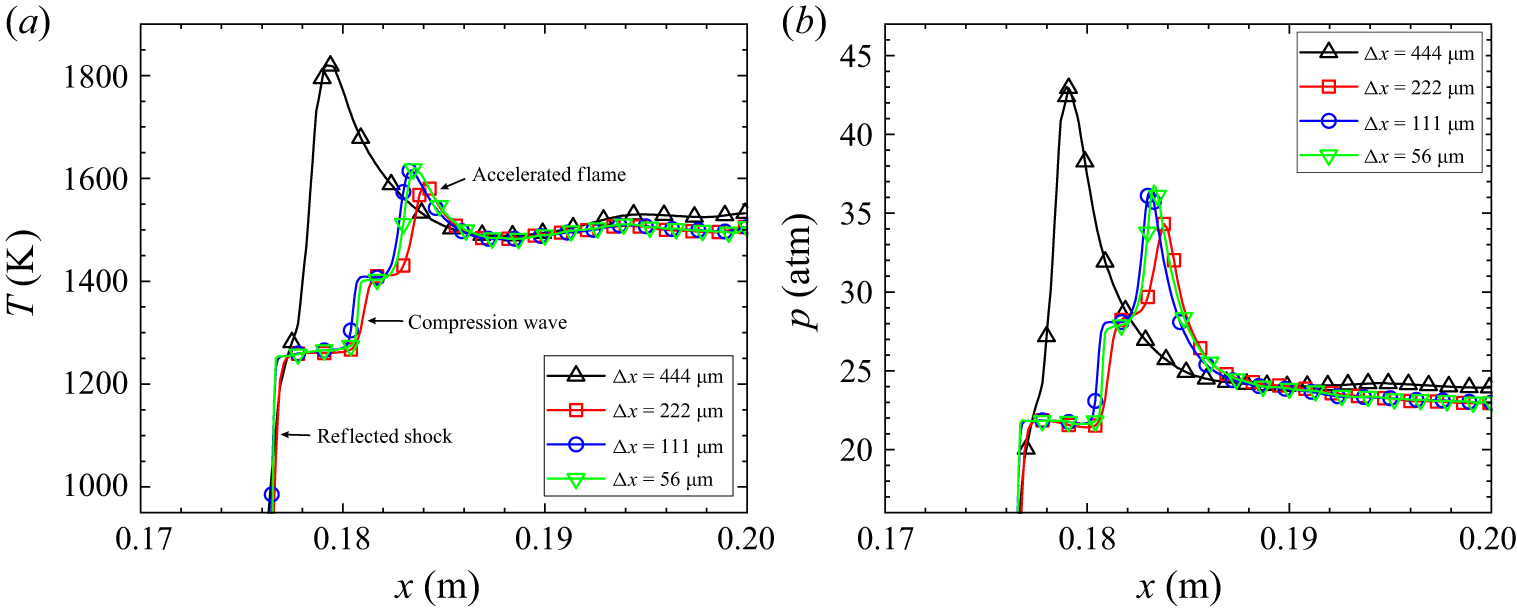
To assess the accuracy of the current grid resolution in simulating reactive RMI, a grid convergence study is performed. Figure 6 compares pressure and temperature profiles along the centreline for the reactive RMI case of
 ${\textit{Ma}}=1.83$
at
 $t = 560\,\unicode {x03BC}\text{s}$
using four different grid sizes, ranging from
 $\Delta x = 444\,\unicode {x03BC}\text{m}$
to
 $\Delta x = 56\,\unicode {x03BC}\text{m}$
. The region from
 $x = 0.17\,\text{m}$
to
 $x = 0.20\,\text{m}$
reveals the complex flow structures including the reflected shock, compression wave and accelerated flame. As the grid is refined, the pressure and temperature profiles converge, indicating improved consistency in the timing and location of ignition. Results for
 $\Delta x = 111\,\unicode {x03BC}\text{m}$
closely match those for
 $\Delta x = 56\,\unicode {x03BC}\text{m}$
, suggesting sufficient resolution. To balance computational accuracy and efficiency, a grid size of
 $\Delta x = 100\,\unicode {x03BC}\text{m}$
is adopted in this study. While key centreline quantities, including temperature, pressure, velocity and species densities, exhibit good convergence, the current grid resolution remains insufficient to fully capture the small-scale turbulent structures that usually emerge at later stages (Collins & Jacobs Reference Collins and Jacobs2002). Capturing the fully developed turbulent mixing at later stages would require a substantially finer grid and a much longer simulation time. Moreover, accurately resolving small-scale turbulence demands not only high spatial resolution but also numerical schemes with good spectral properties, as discussed in our recent studies on turbulent mixing (Zhou et al. Reference Zhou, Ding, Huang and Luo2023b
, Reference Zhou, Ding and Cheng2024). We note that resolving the detailed turbulent mixing is beyond the scope of the present work.
Comparisons of centreline temperature (a) and pressure (b) profiles using four different grid resolutions for the
 ${\textit{Ma}} = 1.83$
case at
 $t = 560\ \unicode {x03BC}\text{s}$
.

4.3. Flow structures under various Mach numbers
In this work we systematically investigate the reactive RMI over a broad range of incident shock Mach numbers (
 $1.20 \lt Ma \lt 3.00$
), along with their inert counterparts for comparison. To isolate the effects of chemical reactions, the same numerical framework and initial conditions are employed for both cases. The reaction computation step in the code is explicitly disabled in the inert case, while it remains active in the reactive case. All simulations adopt the same mixture components, namely H
 $_2$
/O
 $_2$
/Xe = 2 : 1 : 97 by volume. Four distinct regimes are identified within the subrange
 $1.70 \lt Ma \lt 2.60$
, each characterised by varying degrees of interaction between chemical reactions and hydrodynamic instabilities, leading to different perturbation growth patterns. These include an inert regime (
 ${\textit{Ma}} \lt 1.80$
) where chemical reactions have minimal impact on interface dynamics, a deflagration regime (
 $1.80 \lt Ma \lt 1.86$
) characterised by multiple shock–interface interactions, a detonation regime (
 $1.86 \lt Ma \lt 2.50$
) characterised by a single strong detonation wave that subsequently interacts with the interface and an immediate detonation regime (
 ${\textit{Ma}} \gt 2.50$
) where ignition occurs immediately after the incident shock impact. Each regime exhibits unique patterns of ignition timing, wave propagation and interface dynamics.
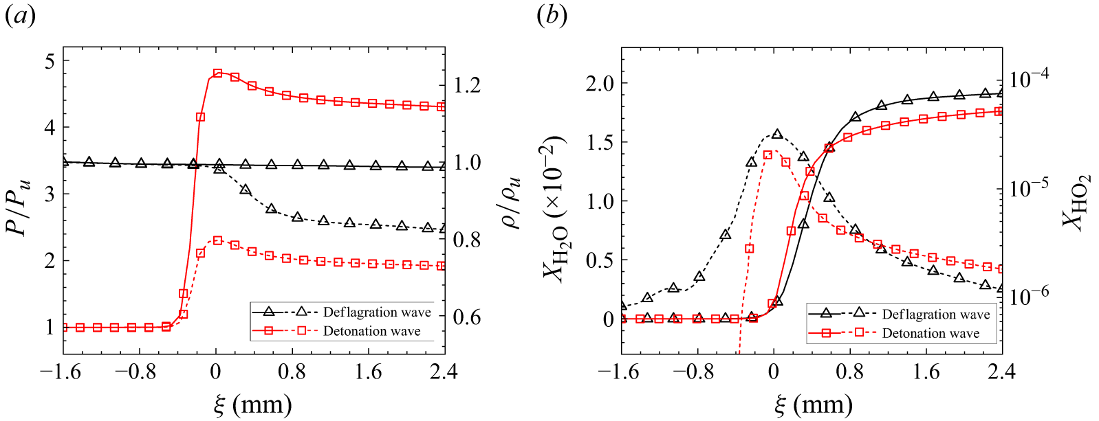
Before analysing these regimes, it is essential to accurately identify reaction wave types, as this is a critical foundation for analysing reactive flows. To establish a criterion for distinguishing deflagration and detonation waves, a detailed examination of their characteristic thermodynamic and chemical properties across the reaction zone is conducted. Figure 7 presents a comparative analysis of the spatial distributions of density ratio (
 $\rho /\rho _u$
), pressure ratio (
 $P/P_u$
) and volume fractions of
 $\text{H}_2\text{O}$
and
 $\text{HO}_2$
in the vicinity of the flame for both wave types, where the subscript
 $u$
denotes the unburnt gas. The data are taken from a deflagration wave in the
 ${\textit{Ma}} = 1.80$
case (
 $t = 700$
 $\unicode {x03BC}\text{s}$
) and a detonation wave in the
 ${\textit{Ma}} = 2.0$
case (
 $t = 500$
 $\unicode {x03BC}\text{s}$
). Here, the volume fraction of H
 $_2$
O serves as an indicator of reaction progress, while the volume fraction of HO
 $_2$
represents reaction intensity. As shown in figure 7(a), the deflagration wave maintains an approximately constant pressure across the flame whereas the detonation wave exhibits a sharp rise in pressure immediately behind the flame, followed by a gradual decay. In both waves, the density exhibits a noticeable drop across the flame. Figure 7(b) shows that in the deflagration case, preheating of the unburnt gas facilitates the gradual formation of
 $\text{HO}_2$
radicals ahead of the flame front, resulting in a peak concentration near the flame front and reduced levels on both sides. In contrast, in the detonation case, the rapid and intense energy release immediately behind the flame front induces an abrupt rise in
 $\text{HO}_2$
concentration, while its level remains nearly zero in the pre-flame region. The distribution of the product species
 $\text{H}_2\text{O}$
is similar in both cases: its concentration remains near zero ahead of the flame front and rises sharply across the flame. However,
 $\text{H}_2\text{O}$
accumulates more slowly in the detonation wave than in the deflagration case, suggesting a longer equilibration process behind the detonation wave. These distinctly different distributions of thermodynamic and chemical parameters provide a clear and reliable basis for distinguishing between deflagration and detonation waves in the present simulations.
Spatial distributions of pressure, density and gas compositions across deflagration and detonation waves. The subscript
 $u$
denotes the unburnt gas state. The coordinate
 $\xi$
is defined in the reference frame moving with the reaction wave. Panel (a) shows the pressure ratio (solid line) and density ratio (dotted line), while panel (b) presents the volume fractions of H
 $_2$
O (solid line) and HO
 $_2$
(dotted line).

4.3.1. Inert regime
At lower Mach numbers (
 ${\textit{Ma}} \approx 1.80$
and below), the ignition delay time of the reshocked premixed gas significantly exceeds the characteristic flow time scale. This substantial delay leaves chemical reactions largely inactive during the primary stages of instability development. Figure 8 shows the interface evolution and shock propagation at
 ${\textit{Ma}} = 1.80$
. It should be noted that the schlieren images presented here are pseudo-schlieren images generated from simulation data. This case provides a representative example of the characteristic flow behaviour in this regime. To highlight the influence of chemical reactions, each panel displays the reactive case above the symmetry axis and the corresponding inert case below it for direct comparison. As the incident shock interacts with the interface, it splits into a transmitted shock propagating forward and a reflected shock propagating backward (50
 $\unicode {x03BC}\text{s}$
). As time proceeds, the shocked interface distorts considerably, forming asymmetric bubble–spike structures (600
 $\unicode {x03BC}\text{s}$
). The bubble refers to the region where a light fluid rises into a heavy fluid, while the spike represents the penetration of a heavy fluid into a light fluid. Later, the transmitted shock reflects off the right boundary as a backward-moving reflected shock that subsequently re-impacts the interface at around
 $650\ \unicode {x03BC}\text{s}$
, generating a rarefaction wave and a second transmitted shock. It is observed that ignition occurs at the corner of the end wall at approximately
 $750 \ \unicode {x03BC}\text{s}$
, followed by a slowly propagating flame, attributed to the relatively low reaction rate. Also, by 1000
 $\unicode {x03BC}\text{s}$
, complex wave interactions give rise to localised high-temperature and high-pressure regions near the bubbles, triggering ignition there. Overall, owing to the substantial ignition delay and the low reaction rate, chemical reactions exert minimal influence on the interface evolution in this regime. This is evidenced in figure 8(a), where the interface morphology and wave patterns in the reactive case closely resemble those of the inert case during the whole evolution process. Similarly, the temperature distribution remains comparable between the reactive and non-reactive cases, as illustrated in figure 8(b). Since chemical reactions exert negligible influence on the flow field at this Mach number and below, this regime is classified as the inert regime.
(a) Pseudo-schlieren images overlaid with contours of the volume fraction of H
 $_2$
O, and (b) temperature contours for both reactive and non-reactive RMI at
 ${\textit{Ma}} = 1.80$
. Each panel displays the reactive case (above the symmetry axis) and the non-reactive case (below the symmetry axis).

A visible asymmetry is observed in the flow structures at
 $t=2000$
 $\unicode {x03BC}$
s for both the inert and reactive cases. Previous studies have shown that vortex structures induced by RMI become highly unstable at later stages (Fleischmann, Adami & Adams Reference Fleischmann, Adami and Adams2019), and even very small numerical perturbations or round-off errors can produce asymmetries. Such numerical asymmetry is a well-known phenomenon in high-accuracy simulations and has been widely observed in both non-reactive and reactive RMI cases (Latini et al. Reference Latini, Schilling and Don2007a
; Jiang et al. Reference Jiang, Dong, Chen and Li2016a
). Although the asymmetry observed in the present simulations arises primarily from numerical effects, it should be emphasised that similar asymmetries commonly occur in physical experiments, as perfectly symmetric conditions are practically unattainable.
4.3.2. Deflagration regime
As the Mach number increases (
 ${\textit{Ma}} \approx 1.80{-}1.86$
), the ignition delay time decreases significantly, and combustion begins to exert an earlier and noticeable influence on interface evolution. Figure 9 illustrates this regime using the representative case of
 ${\textit{Ma}} = 1.83$
. The early stage interface evolution in the reactive case resembles that of the inert case, but noticeable divergence is observed at later times (
 $t \gt 680\ \unicode {x03BC}\text{s}$
). After the reflected shock heats the combustible gas to a high temperature, ignition occurs at the corner of the right wall (
 $t=560$
 $\unicode {x03BC}$
s). Unlike the inert regime at
 ${\textit{Ma}} = 1.80$
, intensified combustion in this case continuously accelerates the flame fronts and generates a compression wave that nearly steepens into a shock at
 $t = 630$
 $\unicode {x03BC}$
s, propagating behind the reflected shock. After the reflected shock re-impacts the interface, the interface amplitude reduces quickly to zero (i.e. phase inversion) and then grows persistently with an opposite phase. Also, this interaction generates a backward-propagating rarefaction wave and a forward-moving transmitted shock. The rarefaction wave subsequently interacts with the flame, decelerating its propagation in the central region, thereby distorting the flame shape (680
 $\unicode {x03BC}\text{s}$
). Later, the combustion-induced shock wave impinges upon the evolving interface, further accelerating instability development. During this process, a third transmitted shock is generated, which quickly overtakes and merges with the second one, forming a stronger combined transmitted shock with a faster speed compared with that in the inert case (800
 $\unicode {x03BC}$
s). Owing to interface deformation, which disperses the premixed gas along the evolving interface, and the emergence of complex wave patterns, particularly rarefaction waves that reduce temperature and pressure, residual pockets of unburnt premixed gas are observed at
 $t = 1000$
 $\unicode {x03BC}\text{s}$
. These pockets progressively diminish as the reaction proceeds, with complete combustion occurring around
 $t = 2000$
 $\unicode {x03BC}\text{s}$
. The present result indicates that combustion is strongly modulated by the interface dynamics and wave patterns. In turn, heat release and gas expansion from combustion lead to a significantly greater interface amplitude in the reactive case than in the inert case (
 $1000\ \unicode {x03BC}\text{s}$
). Additionally, due to localised heat release caused by combustion, a smaller secondary spike appears at the tip of the primary spike in the reactive case (
 $t = 2000$
 $ \unicode {x03BC}\text{s}$
), revealing the pronounced influence of combustion on interface dynamics. It is worth emphasising that this case exhibits sustained coupling between reaction kinetics and interface dynamics throughout the entire evolution process.
(a) Pseudo-schlieren images overlaid with contours of the volume fraction of H
 $_2$
O, and (b) temperature contours for both reactive and non-reactive RMI at
 ${\textit{Ma}} = 1.83$
. Each panel displays the reactive case (above the symmetry axis) and the non-reactive case (below the symmetry axis).

4.3.3. Detonation regime
At higher Mach numbers (
 ${\textit{Ma}} \approx 1.86{-}2.50$
), the ignition delay time further decreases and the deflagration wave transitions into a detonation wave. Figure 10 illustrates this scenario at
 ${\textit{Ma}}=2.0$
, where ignition occurs shortly after the formation of the reflected shock (440
 $\unicode {x03BC}\text{s}$
). In this case, more intense combustion allows the flame to rapidly catch up with both the pressure wave and the reflected shock ahead of it, merging into a detonation wave before reaching the interface (
 $510\ \unicode {x03BC}\text{s}$
). Note this detonation wave re-impacts the interface only once at approximately
 $t = 520\ \unicode {x03BC}\text{s}$
, in contrast to the deflagration regime, where the reflected shock and the combustion-induced pressure wave successively strike the interface. After the reshock event, the combustible gas is completely consumed, leaving no residual unburnt gas (580
 $\unicode {x03BC}$
s). Due to the stronger impact by the detonation wave and the quick expansion of the burnt gases, the interface evolves more rapidly following reshock compared with the inert case. Owing to the quick consumption of the premixed gas, the morphology of the spike at late stages suffers minimal influence from combustion, exhibiting behaviour similar to that in the inert case. Also, combustion is relatively strong in this regime and suffers minimal influence from the flow dynamics. Overall, the interplay between combustion and flow dynamics in this regime is relatively weak compared with the deflagration regime, despite the higher Mach number. It should be noted that when the Mach number reaches approximately 2.45, ignition occurs near the spike structures after the incident shock passes through the interface. However, due to the relatively low temperature and pressure behind the incident shock, the combustion proceeds slowly, resulting in a weaker influence on the flow compared with combustion occurring behind the reflected shock. As a result, the subsequent instability evolution remains qualitatively similar to that observed at lower Mach numbers, and this scenario is therefore still categorised within the detonation regime.
(a) Pseudo-schlieren images overlaid with contours of the volume fraction of H
 $_2$
O, and (b) temperature contours for both reactive and non-reactive RMI at
 ${\textit{Ma}} = 2.00$
. Each panel displays the reactive case (above the symmetry axis) and the non-reactive case (below the symmetry axis).

4.3.4. Immediate detonation regime
At very high Mach numbers (
 ${\textit{Ma}} \approx 2.50$
and above), the ignition delay time significantly decreases and detonation occurs behind the incident shock. Figure 11 illustrates this scenario using the representative case of
 ${\textit{Ma}} = 2.60$
. Shortly after the incident shock passes across the interface, a pressure wave emerges ahead of the flame front, closely following the transmitted shock (90
 $\unicode {x03BC}\text{s}$
). Before reaching the wall boundary, the flame overtakes the pressure wave and the transmitted shock, generating a stronger forward-propagating detonation wave (approximately 130
 $\unicode {x03BC}\text{s}$
). Complex transverse wave patterns develop behind the detonation front, which is a typical manifestation of detonation instability (
 $t=280\,\unicode {x03BC}\text{s}$
). Characteristic detonation features, including triple points of shock waves, Mach stems, transverse shocks and decoupled reaction zones, become distinctly visible, which align qualitatively with previous numerical simulations (Oran et al. Reference Oran, Weber, Stefaniw, Lefebvre and Anderson1998) and experimental observations (Voitsekhovskii, Mitrofanov & Topchiyan Reference Voitsekhovskii, Mitrofanov and Topchiyan1969). Subsequently, the detonation wave reflects off the end wall and interacts with the deforming interface, significantly altering its evolution (
 $t = 330$
 $\unicode {x03BC}\text{s}$
). In the early stages after reshock (800
 $\unicode {x03BC}\text{s}$
), the overall interface width is smaller than in the inert case due to the stronger compression induced by the detonation wave. At later times (2000
 $\unicode {x03BC}\text{s}$
), however, the interface becomes wider than in the inert case due to the enhanced deposition of baroclinic vorticity that drives instability development. The spike also exhibits markedly different morphologies compared with the inert scenario, which is attributed to the increased transverse waves behind the detonation front. To facilitate direct comparison of the interface evolution under different Mach numbers, figure 12 presents a comparative overview of the reactive-interface evolution across the four regimes.
(a) Pseudo-schlieren images overlaid with contours of the volume fraction of H
 $_2$
O, and (b) temperature contours for both reactive and non-reactive RMI at
 ${\textit{Ma}} = 2.60$
. Each panel displays the reactive case (above the symmetry axis) and the non-reactive case (below the symmetry axis).

Comparison of interface evolution across different regimes.

5. Quantitative analyses
5.1. Mixing width
The mixing width, i.e. the total width of the mixing layer, is a quantity of great interest in the RMI community. Following Zhou et al. (Reference Zhou, Ding, Cheng and Luo2023a ), the mixing width is calculated as
 \begin{equation} W_f = \int 4 \langle X_{\text{N}_2} \rangle _y \langle 1-X_{\text{N}_2} \rangle _y \,\text{d}x, \end{equation}
where
 $\langle \boldsymbol{\cdot }\rangle _y$
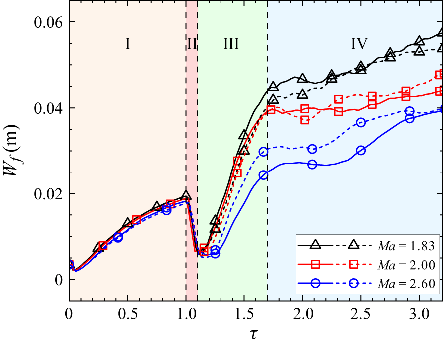
denotes spanwise averaging. Figure 13 illustrates the temporal variation of mixing width for both reactive and inert cases across different Mach numbers. Here, time is non-dimensionalised as
 $\tau = t / t_{{reshock}}$
, with
 $t_{{reshock}}$
denoting the instant at which the reflected shock interacts with the interface. Unless otherwise specified, time is normalised in this way throughout the remainder of this work. Across all cases, the mixing width follows a consistent overall evolution pattern that can generally be divided into four distinct stages. Following the impact of the incident shock, the mixing width first experiences a brief reduction due to shock compression and then increases continuously as the interface evolves (stage I,
 $\tau \lt 1.0$
). Later, the reflected shock reaccelerates the interface in the opposite direction, generating baroclinic vorticity of opposite sign compared with that induced by the incident shock, thereby causing a phase inversion. This leads to a rapid decrease in mixing width (stage II,
 $1.0 \lt \tau \lt 1.1$
). Subsequently, the mixing width grows rapidly at a rate exceeding that in stage I (stage III,
 $1.1 \lt \tau \lt 1.7$
). At late stages, the large vortices on both sides of the spike break down, transferring energy to smaller-scale structures that results in a reduced growth rate of the mixing width (stage IV,
 $\tau \gt 1.7$
). The remarkable consistency in the timing of these four stages across different cases highlights the effectiveness and appropriateness of the present non-dimensionalisation approach.
Temporal evolution of the mixing width for three reactive cases (solid line) and their inert counterparts (dotted line). Time is non-dimensionalised as
 $\tau = t / t_{{reshock}}$
, with
 $t_{{reshock}}$
denoting the instant the reflected shock interacts with the interface.

The comparison between reactive and inert cases shows that combustion has minimal impact on mixing width growth in stages I and II, while exerting a noticeable influence in stages III and IV. The growth rate of mixing width in stage III is strongly dependent on the regime that each case belongs to, as discussed in the previous section. Specifically, in the deflagration regime (
 ${\textit{Ma}} = 1.83$
), the mixing width increases significantly after reshock, with a steeper growth rate than in the inert case. However, in the detonation regime (
 ${\textit{Ma}} = 2.0$
), both the reactive and inert cases exhibit nearly identical post-reshock growth rates, with slopes obtained from linear fits of 0.077 and 0.078 for the inert and reactive cases, respectively. This finding is consistent with the observation presented earlier regarding the influence of combustion on flow structures. In the immediate detonation regime (
 ${\textit{Ma}} = 2.60$
), the reactive case initially exhibits a markedly lower post-reshock growth rate than the inert case. Despite the deviation observed in stage III, the mixing width ultimately converges to a comparable level in stage IV for both reactive and inert cases, illustrating that the influence of combustion diminishes at late stages as the fuel is depleted. The present analysis highlights the complex interplay between reactive and hydrodynamic effects in reactive RMI, revealing how the intensity of combustion fundamentally alters the mixing zone development.
It is also observed that the interface width at late times in the
 ${\textit{Ma}} = 2.6$
case is smaller than that in the other two cases. Three factors contribute to this phenomenon. First, in the
 ${\textit{Ma}} = 2.6$
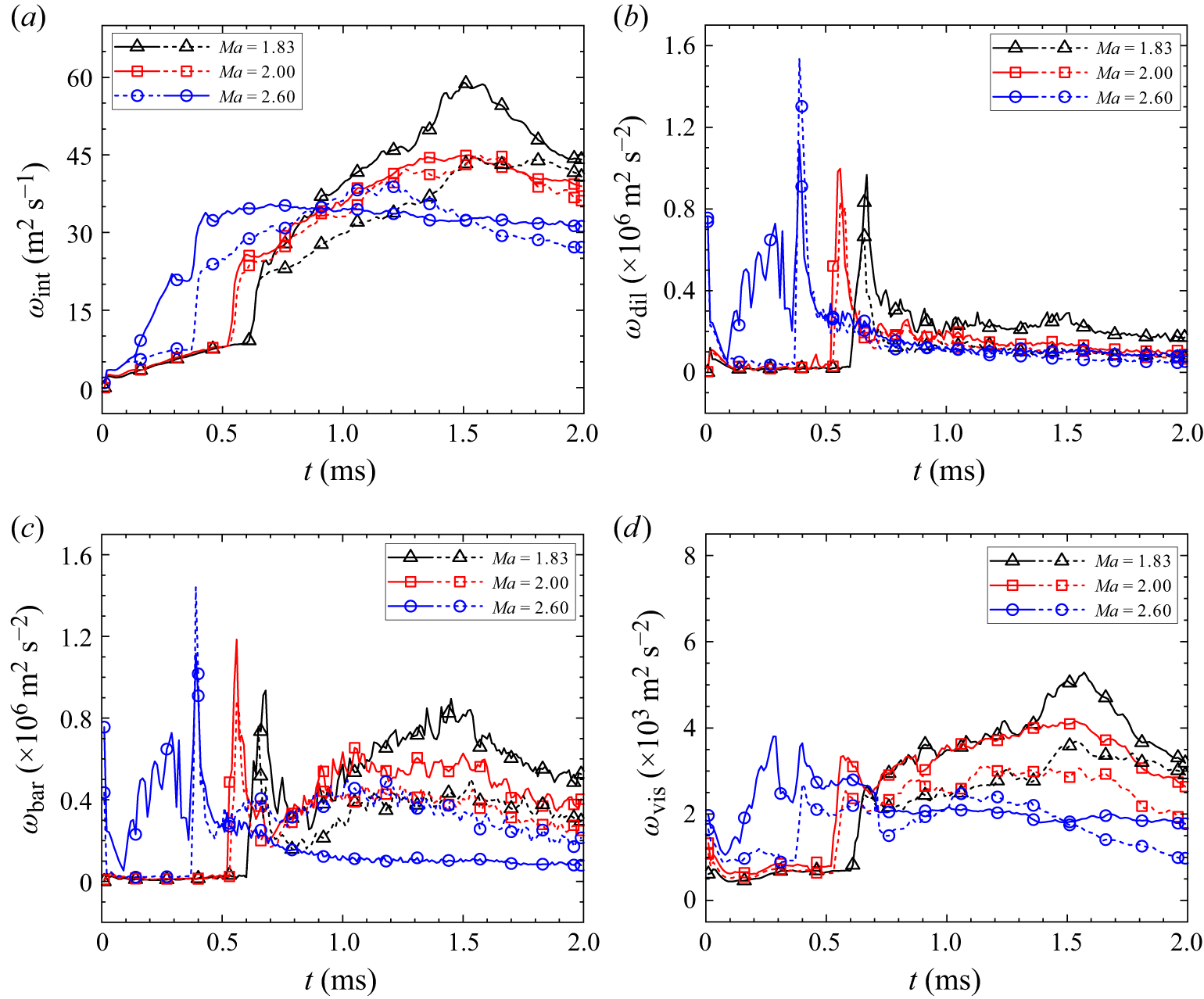
case, detonation occurs immediately after the incident shock. Before the reflected detonation wave re-impacts the interface, the density ratio across the interface becomes smaller than in the other cases, reducing baroclinic vorticity generation. As shown in figure 18(c), the
 ${\textit{Ma}} = 2.6$
reactive case exhibits a notably lower peak vorticity from reshock compared with the
 ${\textit{Ma}} = 2.0$
case. Second, a detailed examination of each term in the vorticity transport equation in § 5.6 reveals that in compressible flows, particularly at high Mach numbers, the dilatational term is nearly as significant as the baroclinic term, indicating that overall vorticity dynamics cannot be attributed solely to baroclinic effects. Third, stronger shocks induce greater compression of the fluid. Schlieren images show that at higher Mach numbers, the shocked interface remains closer to the wall, reflecting stronger compression of the perturbation amplitude.
5.2. Mixed mass
Following the recommendation of Zhou et al. (Reference Zhou, Cabot and Thornber2016, Reference Zhou, Groom and Thornber2020), the normalised mixed mass,
 $\psi$
, is calculated to quantify the mixing degree within the mixing zone. It is defined as
 \begin{equation} \psi = \frac {\int \langle \rho Y_{\text{N}_2} (1 - Y_{\text{N}_2}) \rangle _y\, \text{d}x} {\int \langle \rho \rangle _y \langle Y_{\text{N}_2} \rangle _y \langle (1 - Y_{\text{N}_2}) \rangle _y\, \text{d}x}. \end{equation}
Here,
 $\psi =1$
represents a homogenised molecular mixing, while
 $\psi =0$
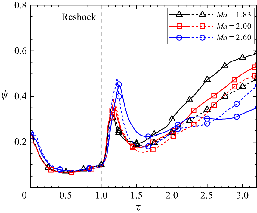
represents a completely entrained flow. Figure 14 presents the variation of the normalised mixed mass with dimensionless time for both reactive and inert cases across various Mach numbers. Following shock impact,
 $\psi$
decays rapidly due to the expansion of the mixing layer. As
 $\tau$
approaches 0.3,
 $\psi$
approaches a plateau, indicating that the growth rate of the mixing width becomes comparable to the molecular mixing rate. At
 $\tau = 1.0$
, the reflected shock strikes the interface, simultaneously enhancing the molecular mixing rate and meanwhile compressing the interface width, thereby causing a rapid rise in mixed mass. Around
 $\tau = 1.2$
when the phase inversion completes, the interface width grows rapidly in an opposite direction, leading to a quick decrease in mixed mass. The apparent decrease in mixed mass is closely related to the fact that the flow remains largely in a single-mode and non-turbulent regime during the observed period. This behaviour can be understood by examining the definition of the dimensionless mixed mass. The dimensionless mixed mass
 $\psi$
, defined in (5.2), is intended to quantify the degree of mixing within the mixing zone, rather than the absolute amount of mixed fluid. From a physical standpoint, the dimensional mixed mass integrated over the entire flow domain increases monotonically with time, as molecular mixing continuously proceeds. In contrast, the normalised parameter
 $\psi$
represents the ratio between the actual molecular mixing and a reference state corresponding to complete mixing at the instantaneous mixing zone width, and is therefore inherently sensitive to the evolution of the mixing zone width. The observed decrease in
 $\psi$
after reshock is attributed to the rapid expansion of the mixing zone width following phase inversion, which increases the denominator in (5.2). Since the molecular mixing process cannot keep pace with the rapid expansion of the mixing zone, the normalised mixed mass
 $\psi$
correspondingly decreases. After
 $\tau \approx 1.5$
, large-scale vortices break down into smaller structures, which enhances molecular mixing while suppressing the growth rate of the mixing width (figure 13). As a result, the mixed mass continues to increase slowly until the end of the simulation.
Temporal evolution of mixed mass for reactive cases (solid lines) and their inert counterparts (dotted lines) across different Mach numbers. Time is non-dimensionalised in the same manner as in figure 13.

At
 ${\textit{Ma}} = 1.80$
, the combustion process is relatively weak and has minimal impact on mixing, resulting in a similar evolution pattern of
 $\psi$
in both the reactive and inert cases (not shown in figure 14). In the deflagration regime (
 ${\textit{Ma}} = 1.83$
), the reactive and inert cases exhibit similar mixing behaviour for
 $\tau \lt 1.5$
, beyond which the reactive case shows significantly enhanced mixing. This enhancement is primarily due to the prolonged interaction between combustion and flow dynamics in this regime, particularly at later stages where combustion induces the formation of secondary spikes, leading to increased surface area and small-scale structures. In the detonation regime (
 ${\textit{Ma}} = 2.0$
), the reactive case also exhibits higher mixing compared with its inert counterpart at late stages (
 $\tau \gt 1.5$
), although the deviation between the two is less pronounced than in the
 ${\textit{Ma}} = 1.83$
case. This suggests that, despite being stronger, the single combined wave at
 ${\textit{Ma}} = 2.0$
, formed by the detonation wave overtaking and merging with the reflected shock, has a weaker impact on mixing than the sequential interaction of the reflected shock and pressure wave in the deflagration regime. This is consistent with the qualitative observations of interface morphology discussed in § 4.3, where the spike structures at late times differ significantly between the reactive and inert cases at
 ${\textit{Ma}} = 1.83$
, but remain similar at
 ${\textit{Ma}} = 2.0$
. At
 ${\textit{Ma}} = 2.60$
, detonation is initiated shortly after the incident shock interacts with the interface, resulting in an earlier divergence between the reactive and inert cases (
 $\tau \gt 1.0$
). At later stages, the reactive case exhibits a lower degree of mixing than the inert case, as intense combustion has consumed many small-scale structures that would otherwise promote molecular mixing. Differing from the findings of Diegelmann et al. (Reference Diegelmann, Hickel and Adams2016a
), who found that combustion waves generally suppress mixing, our results reveal that the influence of combustion on mixing is more complex and strongly dependent on the flow regime.
5.3. Internal energy
Prior to ignition, the premixed gases continuously absorb energy from the surrounding flow, primarily from shock waves, resulting in the accumulation of radical species in regions of high pressure and temperature. Once a critical concentration of radicals is reached, ignition occurs. Afterwards, substantial chemical energy is released back into the flow, causing a significant increase in temperature (i.e. internal energy). Hence, the total internal energy serves as an effective indicator for characterising the chemically reacting flow state, as it captures both the energy absorption during the induction period and the subsequent heat release during combustion. Following the methodology of Yan et al. (Reference Yan, Fu, Wang, Yu and Li2022a ), we define the total internal energy of the reactive gas mixture and the heat release rate as
 \begin{align} E_i&=\iint _{S} \sum _{i=1}^{ns_r}(\rho _i h_i - p) {\rm d}S, \end{align}
 \begin{align} Q_s&=\iint _{S} \sum _{i=1}^{ns_r}( - \dot {\omega _i} h_{i0}) {\rm d}S, \end{align}
where S denotes the entire computational domain. Here,
 $ns_r$
represents all species excluding the inert gases (
 $N_2$
and
 $Xe$
) and
 $h_{i0}$
denotes the heat of formation of the
 $i$
th species, computed as the product of
 $R_i$
and
 $F_i$
.
Figure 15(a) shows the evolution of total internal energy with dimensionless time for all cases. Both reactive and inert cases exhibit a similar evolution pattern, which can be characterised by four stages. As the incident shock traverses the interface and enters the combustible gas, it continuously heats the combustible gas, resulting in a sustained rise in internal energy (stage I). Once the reflected shock forms and propagates through the combustible gas, the associated temperature rise accelerates the increase of internal energy (stage II). At
 $\tau =1.0$
, when the reflected shock has fully compressed the combustible gas, the internal energy reaches its peak value. Simultaneously, the reflected shock–interface interaction generates a rightward-propagating rarefaction wave, which reduces the temperature of the combustible gas and consequently reduces the internal energy (stage III). Around
 $\tau = 1.5$
, when the rarefaction wave reflects from the wall and reinteracts with the interface, the internal energy remains nearly constant (stage IV), indicating that the subsequent waves are too weak to have a significant impact on internal energy.
Temporal evolution of internal energy: (a) comparison between reactive cases (solid lines) and inert cases (dotted lines), and (b) their difference for four different Mach numbers.

In the inert regime (
 ${\textit{Ma}} = 1.80$
), combustion proceeds slowly and has minimal impact on the flow, resulting in only minor differences between the reactive and inert cases. In the deflagration regime (
 ${\textit{Ma}} = 1.83$
), ignition occurs approximately when the reflected shock reaches the interface, leading to a higher total internal energy in the reactive case after reshock. In this regime, ignition occurs before the reflected shock reaches the interface, leading to an accelerated rise in internal energy, as shown in the zoomed view in figure 15(a). This explains the distinct slope increase in the internal energy profile prior to reshock. At
 ${\textit{Ma}} = 2.0$
(detonation regime), ignition occurs earlier, leading to an earlier and more pronounced deviation in internal energy between the reactive and inert cases. At
 ${\textit{Ma}} = 2.60$
(immediate detonation regime), combustion is initiated almost immediately after the incident shock passes the interface, leading to a steeper rise in internal energy from the beginning. Among all Mach number cases, this scenario exhibits the most significant discrepancy between the reactive and inert cases. Overall, the total internal energy is consistently higher in the reactive case, with the deviation from the inert case becoming more pronounced at higher Mach numbers, as shown in figure 15(b).
5.4. Heat of formation and heat release rate
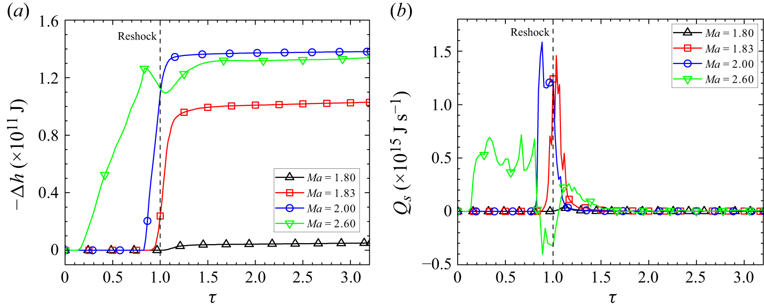
Figure 16 illustrates the temporal evolution of heat of formation and heat release rate across the four Mach numbers. As shown in figure 16(a), the total energy released into the flow via combustion increases with Mach number from 1.80 to 2.00, indicating more complete combustion at higher Mach numbers. However, despite an earlier onset of heat release, the total heat of formation in the
 ${\textit{Ma}} = 2.60$
case is lower than that in the
 ${\textit{Ma}} = 2.00$
case. This suggests that the high-temperature chemical dissociation in the
 ${\textit{Ma}} = 2.60$
case is more significant than in the
 ${\textit{Ma}} = 2.00$
case, leading to a lower heat of formation. Specifically, when the temperature exceeds a critical threshold, reverse reactions dominate, leading to H
 $_2$
O dissociation into radicals and a corresponding reduction in heat formation.
Temporal evolution of (a) heat of formation and (b) heat release rate for reactive RMI across four different Mach numbers.

Figure 16(b) shows that in the detonation regime (
 ${\textit{Ma}} = 2.00$
), the majority of chemical energy is released into the flow prior to reshock, whereas in the deflagration regime (
 ${\textit{Ma}} = 1.83$
), more than half is released after reshock. The former also exhibits a relatively higher peak heat release rate, primarily due to elevated temperature and pressure near the wall, which cause faster reactions. By
 $\tau = 1.5$
, the heat release rate becomes negligible for both cases, indicating near-complete combustion under favourable conditions. In the immediate detonation regime (
 ${\textit{Ma}} = 2.60$
), a non-monotonic trend emerges where the heat release rate is lower than that observed at
 ${\textit{Ma}} = 1.83$
and
 ${\textit{Ma}} = 2.00$
. Although the heat release rate initially increases shortly after the incident shock impact, it subsequently declines and even becomes negative before reshock. These unexpected behaviours are attributed to the temperature-dependent nature of the H
 $_2$
O system’s chemical equilibrium state. When the temperature exceeds a critical threshold, reverse reactions become dominant, causing H
 $_2$
O to dissociate into radicals and resulting in negative heat release rates as the system absorbs energy rather than releasing it. Consequently, despite the stronger shock in the
 ${\textit{Ma}} = 2.60$
case, the total accumulated heat release is ultimately lower than that in the
 ${\textit{Ma}} = 2.00$
case. This reversal highlights the impact of high-temperature chemical dissociation on limiting the net heat output in high-Mach-number reactive flows.
5.5. Enstrophy
Baroclinic vorticity is one of the driving forces for RMI. Following the approaches of Diegelmann et al. (Reference Diegelmann, Hickel and Adams2016a
) and Zhou, Groom & Thornber (Reference Zhou, Groom and Thornber2020), vorticity can be quantified using enstrophy
 $(\varepsilon )$
, defined as
 \begin{equation} \varepsilon (t) = \iint _{S} \omega ^2\, \text{d}S, \end{equation}
where
 $\omega$
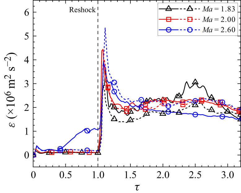
is the vorticity. Figure 17 presents the temporal evolution of enstrophy for both reactive and inert cases across different Mach numbers. Note that the
 ${\textit{Ma}} = 1.80$
case is excluded from the figures due to the weak coupling between chemical reactions and flow. For the
 ${\textit{Ma}} = 1.83$
and
 ${\textit{Ma}} = 2.0$
cases, enstrophy remains relatively low in the early stages, followed by a sharp increase after reshock and a gradual decline before reaching a steady level. In contrast, the
 ${\textit{Ma}} = 2.60$
case exhibits pronounced enstrophy growth prior to reshock, primarily due to the early onset of detonation. Specifically, the numerous transverse waves formed behind the detonation front promote vorticity generation throughout the flow field, as further discussed in § 5.6. In general, the reactive cases exhibit enstrophy evolution patterns similar to their inert counterparts, except at
 ${\textit{Ma}} = 2.60$
. At
 ${\textit{Ma}} = 2.00$
, although the reflected shock evolves into a stronger detonation wave, the overall enstrophy remains comparable to that of the inert case due to the balance between two competing effects. The comparable enstrophy between reactive and inert cases at
 ${\textit{Ma}} = 2.0$
is likely due to two mechanisms: (i) combustion consumes small-scale vortical structures, reducing local vorticity; and (ii) dilatational effects from combustion-induced expansion alter vorticity distribution, as discussed in § 5.6. At
 ${\textit{Ma}} = 2.60$
, intensified heat release prior to reshock reduces the peak enstrophy relative to the inert case, with the subsequent enstrophy level remaining consistently lower than that of the inert case.
Temporal evolution of enstrophy for three reactive cases (solid line) and their inert cases (dotted line).

5.6. Vorticity generation and evolution
The development of RMI is primarily driven by baroclinic vorticity deposited at the interface due to the misalignment between the pressure gradient across the shock and the density gradient at the interface. The dynamics of vorticity are governed by the vorticity transport equation, which is derived by taking the curl of the momentum equations (Wang et al. Reference Wang, Yu, Chen, Zhang and Liu2018; Singh, Battiato & Myong Reference Singh, Battiato and Myong2021; Alsaeed & Singh Reference Alsaeed and Singh2024)
 \begin{align} \dfrac {{\rm D} \boldsymbol{\omega }}{{\rm D}t} &= (\boldsymbol{\omega } \boldsymbol{\cdot }\boldsymbol{\nabla }) \boldsymbol{u} - \boldsymbol{\omega } (\boldsymbol{\nabla }\boldsymbol{\cdot }\boldsymbol{u}) + \dfrac {1}{\rho ^2} (\boldsymbol{\nabla }\rho \times \boldsymbol{\nabla }p) + \dfrac {\mu }{\rho } {\nabla} ^2 \boldsymbol{\omega } - \dfrac {\mu }{\rho ^2} (\boldsymbol{\nabla }\rho \times {\nabla} ^2 \boldsymbol{u}) \nonumber\\&\quad - \dfrac {\mu }{3 \rho ^2} (\boldsymbol{\nabla }\rho \times \boldsymbol{\nabla }(\boldsymbol{\nabla }\boldsymbol{\cdot }\boldsymbol{u})), \end{align}
where
 $\boldsymbol{\nabla}$
is the gradient operator,
 $\boldsymbol{u}=(u,v,0)$
is the velocity vector and
 $\boldsymbol{\omega }$
represents the vorticity vector, calculated as
 $\boldsymbol{\omega } = (0,0, {\partial v}/{\partial x}- {\partial u}/{\partial y})$
in our 2-D simulations. The first term on the right-hand side of (5.6) corresponds to vortex stretching, which is absent in 2-D flows. The second term represents vortex dilatation, a mechanism that becomes significant in highly compressible flows. The third term accounts for baroclinic vorticity generation, which plays a dominant role in RMI flows. The final three terms account for viscous effects. Note the reaction source terms in the governing equations (2.1) directly affect only the species and energy equations, indicating that combustion influences vorticity dynamics indirectly by altering the pressure, density and velocity fields.
To quantify the contribution of individual mechanisms to vorticity transport, we spatially integrate each term in (5.6). The spatially integrated vorticity in the whole domain is defined as
 \begin{equation} \omega _{int}(t) = \iint _{S} \| \boldsymbol{\omega } \| {\rm d}S, \end{equation}
where
 $S$
denotes the whole computational domain. The spatially integrated dilatational vorticity is
 \begin{equation} \omega _{dil}(t) = \iint _{S} \| \boldsymbol{\omega } (\boldsymbol{\nabla }\boldsymbol{\cdot }\boldsymbol{u}) \| {\rm d}S, \end{equation}
while the spatially integrated baroclinic vorticity is
 \begin{equation} \omega _{bar}(t) = \iint _{S} \| \dfrac {1}{\rho ^2}(\boldsymbol{\nabla }\rho \times \boldsymbol{\nabla }p) \| {\rm d}S. \end{equation}
The remaining viscous terms are combined into the viscous vorticity, defined as
 \begin{equation} \omega _{vis}(t) = \iint _{S} \| \dfrac {\mu }{\rho } {\nabla} ^2 \boldsymbol{\omega } - \dfrac {\mu }{\rho ^2} (\boldsymbol{\nabla }\rho \times {\nabla} ^2 \boldsymbol{u}) - \dfrac {\mu }{3 \rho ^2} (\boldsymbol{\nabla }\rho \times \boldsymbol{\nabla }(\boldsymbol{\nabla }\boldsymbol{\cdot }\boldsymbol{u})) \| {\rm d}S. \end{equation}
Figure 18 presents the temporal variations of these spatially integrated vorticity quantities at different Mach numbers. The domain-integrated vorticity exhibits a similar trend across all cases. Following incident shock impact, vorticity is rapidly generated at the interface and then gradually accumulates over time. The reflected shock also causes a quick increase in vorticity, followed by a slower growth phase and a gradual decay at later times. Although the overall trend is consistent across different cases, notable differences in vorticity magnitude are observed between reactive and inert cases. For the deflagration regime (
 ${\textit{Ma}} = 1.83$
), the discrepancy becomes apparent after reshock, with the reactive case showing significantly higher vorticity. This enhancement can be attributed to the sequential interaction between the reflected shock and combustion-induced pressure waves with the interface, with the latter depositing additional baroclinic vorticity. In the detonation regime (
 ${\textit{Ma}} = 2.00$
), the domain-integrated vorticity remains comparable between the reactive and inert cases after reshock. This reasonably explains the similar interface evolution and mixing width growth in reactive and inert RMI cases at
 ${\textit{Ma}} = 2.00$
observed earlier. In contrast, for the immediate detonation regime (
 ${\textit{Ma}} = 2.60$
), divergence appears at the early stage, since detonation occurs immediately after the incident shock. Notably, in this regime, the domain-integrated vorticity in the reactive case is significantly higher than that in the inert case before reshock, as the intensified transmitted shock produces slip lines that generate considerable vorticity. The combined viscous term exhibits a similar variation trend to that of the domain-integrated vorticity, but with magnitudes three orders lower, as shown in figure 18(d). This indicates that viscous effects play a negligible role in interface evolution during the time period considered.
Temporal evolution of spatially integrated (a) domain-integrated vorticity, (b) dilatational vorticity, (c) baroclinic vorticity, and (d) viscous vorticity at various Mach numbers. Solid lines denote reactive cases, while dotted lines denote non-reactive cases.

As illustrated in figures 18(b) and 18(c), the spatially integrated dilatational vorticity and baroclinic vorticity exhibit remarkably similar evolution patterns at either Mach number. In inert RMI the incident shock induces an initial peak in both quantities, which subsequently diminishes to near-zero values. The second impact from the reflected shock produces another peak, followed by a gradual decay to very low values. In reactive RMI cases at
 ${\textit{Ma}} = 1.83$
and
 $2.00$
, the second peaks produced by the reflected shock are significantly higher than those in inert RMI. This enhancement is attributed to the interaction between the interface and combustion-induced pressure waves (or a stronger detonation wave), which generates intensified baroclinic vorticity. However, for the reactive RMI at Ma = 2.60, these peaks are unexpectedly lower than in inert RMI. This non-monotonic trend is consistent with that observed in the spatially integrated vorticity mentioned above.
In the
 ${\textit{Ma}} = 2.60$
case, detonation waves are generated shortly after the incident shock crosses the interface, accompanied by complex wave structures and significant changes in flow characteristics, which significantly complicate the flow analysis. Figure 19 illustrates the evolution of vorticity for reactive RMI at
 ${\textit{Ma}}=2.60$
. The localised combustion at the spike tip generates non-planar flame fronts and pressure waves with vertical velocity components. When the flame catches up the transmitted shock, detonation is triggered. By
 $t = 140$
 $\unicode {x03BC}\text{s}$
, a pair of triple points emerges and propagates in opposite directions, accompanied by horizontal wave propagation. Notably, small-scale vortices with embedded jets develop along the slip line, contributing significant vorticity to the bulk flow region. After reshock at
 $t = 210$
 $\unicode {x03BC}\text{s}$
, the slip line becomes unstable and continues moving toward the interface (Oran et al. Reference Oran, Weber, Stefaniw, Lefebvre and Anderson1998). This complex evolution pattern, featuring distinct vorticity generation mechanisms at both the interface and along slip lines, necessitates the separate analysis of vorticity dynamics in these regions as presented in figure 18.
Temporal evolution of vorticity for the reactive case at
 ${\textit{Ma}} = 2.60$
. Each column shows the reactive case (top) and the corresponding non-reactive case (bottom) for comparison.

6. Characteristic time scales
The four regimes observed in § 4 are primarily distinguished by the varying strength and timing of the coupling between hydrodynamic instabilities and chemical kinetics. To characterise the relative importance of chemical reactions compared with hydrodynamic effects, here, we introduce the Damköhler number (
 $\text{Da}$
), which is defined as the ratio of the characteristic hydrodynamic time scale to the chemical reaction time scale. It is formulated as
 \begin{equation} \textit{Da} = \frac {\tau _H}{\tau _C}, \end{equation}
where
 $\tau _C$
represents the characteristic time scale of the chemical reaction, typically approximated by the ignition delay time, while
 $\tau _H$
denotes the characteristic time scale of hydrodynamic instability, which is determined by the dominant physical mechanisms governing instability development. For instance, in reactive shock–bubble interactions (Haehn et al. Reference Haehn, Ranjan, Weber, Oakley, Rothamer and Bonazza2012),
 $\tau _H$
is defined as the ratio of the initial bubble diameter to incident shock velocity, whereas in shock–flame interactions (Jiang et al. Reference Jiang, Dong, Chen and Li2016a
), it is taken as the reciprocal of the spatially averaged vorticity magnitude. In the present study, the flow time scale
 $\tau _H$
is defined as the duration of the shock–interface interaction, as this process directly generates the baroclinic vorticity that drives the interface evolution. Considering that both the incident and reflected shocks contribute to baroclinic vorticity generation upon impacting the interface, the flow time scale
 $\tau _H$
is defined as
 \begin{equation} \tau _H = \begin{cases} L_0/\Delta u & \text{(before the formation of reflected shock)}, \\[5pt] \dfrac {L_1}{u_{T}}\left(\dfrac {u_{T}-\Delta u}{u_{T}+\Delta u}\right) & \text{(after the formation of reflected shock)}, \end{cases} \end{equation}
where
 $\Delta u$
denotes the jump velocity of the interface induced by the incident shock and
 $u_T$
denotes the velocity of the transmitted shock. Also,
 $L_0=40\;\text{mm}$
denotes the characteristic length of the domain and
 $L_1=180\;\text{mm}$
denotes the distance from the initial interface to the end wall.
Detailed hydrodynamic and chemical parameters behind the incident and reflected shocks for reactive cases at various Mach numbers are listed in tables 1 and 2, respectively. It should be emphasised that for high Mach numbers, combustion occurs before the reshock event, while for lower Mach numbers, combustion takes place after reshock. Therefore, the two tables present data at different stages: for high-Mach-number cases, the parameters are measured before reshock, whereas for low-Mach-number cases, they are measured after reshock. Note the chemical time scale is highly sensitive to variations in temperature and pressure, and therefore, decreases more rapidly than the hydrodynamic time scale with increasing Mach number. It is generally found that
 $Da$
increases monotonically with the Mach number, indicating the increasing significance of chemical reactions at higher Mach numbers. For lower-Mach-number cases (
 $Da \lt 1$
), hydrodynamic effects dominate the interface evolution, whereas for higher-Mach-number cases (
 $Da \gt 1$
), chemical reactions play a dominant role in instability development. When
 $Da \approx 1$
, hydrodynamic and chemical effects are of comparable importance in the reactive RMI, indicating a potential transition between different regimes. As illustrated in table 1, following reshock, there exists a critical low-Mach-number threshold around
 ${\textit{Ma}} = 1.80$
, below which combustion effects are minimal, corresponding to the inert regime discussed earlier. At
 ${\textit{Ma}} = 1.83$
, where
 $Da$
approaches 1.0, the hydrodynamic and chemical time scales become comparable, resulting in the strongest and most sustained interaction between flow dynamics and combustion. This finding aligns well with our previous observation of the detonation regime. Similarly, table 2 indicates that, for
 ${\textit{Ma}} \gt 2.30$
, combustion occurs after the incident shock, but with a small
 $Da$
value, resulting in relatively weak effects. When
 ${\textit{Ma}} \gt 2.50$
,
 $Da$
exceeds 1.0, indicating strong chemical reactions, corresponding to our previously described immediate detonation regime. Note the ignition delay is primarily determined by the temperature and pressure of the gas mixture, which are strongly influenced by the incident and reflected shocks. In our simulations, ignition first occurs following the incident shock at approximately
 ${\textit{Ma}}=2.50$
, marking the transition from the deflagration regime (low Mach numbers) to the immediate detonation regime (high Mach numbers). When the incident shock is not sufficiently strong, ignition relies on the additional compression provided by the reflected shock. Tables 1 and 2 encompass all relevant parameter conditions across various Mach numbers. We note that there is no distinct intermediate regime between low and high Mach numbers. The present analysis demonstrates that the different regimes discussed in the previous section can be fundamentally attributed to variations in the Damköhler number. This provides a robust framework for understanding and predicting flow phenomena in reactive RMI.
Detailed parameters after reshock for cases with different initial Mach numbers. The subscript
 $2$
denotes the post-reshock regions,
 $\Delta u$
denotes the averaged jump velocity of the interface caused by the incident shock and
 $u_{T}$
denotes the velocity of the transmitted shock wave;
 $\tau _C$
denotes numerical ignition delay time under corresponding
 $P_2$
and
 $T_2$
conditions, and
 $\tau _H$
denotes hydrodynamic characteristic time determined by (6.2) after the reflected shock reaccelerates the interface.

Detailed parameters before reshock for cases with different initial Mach numbers. The subscript
 $1$
denotes the post-shock regions,
 $\Delta u$
denotes the averaged jump velocity of the interface caused by the incident shock;
 $\tau _C$
denotes numerical ignition delay time under corresponding
 $P_1$
and
 $T_1$
conditions, and
 $\tau _H$
denotes hydrodynamic characteristic time determined by (6.2) after the incident shock passes through the interface.

7. Conclusions
This study presents high-resolution numerical simulations of reactive RMI at a sinusoidal interface between N
 $_2$
and a H
 $_2$
/O
 $_2$
/Xe mixture under reshock conditions, using a newly developed high-order solver. The solver incorporates the Kéromnès mechanism for combustion modelling and a dual-flux algorithm to suppress numerical oscillations at material interfaces. Its performance is validated through a hierarchical set of benchmark tests, from 0-D homogeneous ignition to 1-D detonation propagation and 2-D reactive shock–bubble interactions, demonstrating its accuracy in capturing both detailed chemical kinetics and wave-interface dynamics.
By systematically varying incident shock Mach numbers, we identify four distinct evolution regimes, each characterised by unique coupling mechanisms between combustion and hydrodynamic effects. In the inert regime (
 $ Ma \lt 1.80$
), combustion is initiated long after the onset of RMI and proceeds at an extremely slow rate, resulting in minimal influence on the interface dynamics. In the deflagration regime (
 $1.80 \lt Ma \lt 1.86$
), combustion is strongly influenced by interface deformation and wave patterns, leading to relatively slow but sustained combustion during the entire evolution process. In turn, heat release and gas expansion from combustion significantly enhance instability growth and generate secondary structures, indicating sustained coupling between reactive and hydrodynamic effects. In the detonation regime (
 $1.86 \lt Ma \lt 2.50$
), deflagration rapidly transitions to detonation following the passage of the reflected shock, leading to a single shock–interface interaction during the reshock stage. Although the reaction rates are high, the coupling between flow dynamics and combustion remains moderate, as the rapid completion of burning shortens the period of interaction. For the immediate detonation regime (Ma > 2.50), detonation occurs immediately after the incident shock, generating complex wave patterns. While the early stage interface evolution remains similar to inert cases, significant differences emerge at late times due to the influence of transverse waves following detonation. These observations reveal that stronger combustion does not necessarily result in stronger coupling between hydrodynamic and reactive effects. Notably, the deflagration regime with moderate reaction rates exhibits the most significant flow modifications due to sustained combustion-flow interactions.
The distinct combustion-flow coupling mechanisms in different regimes lead to dramatic differences in key flow metrics, including mixing characteristics, heat release, enstrophy evolution and vorticity transport. The mixing width and mixed mass exhibit distinct regime-dependent trends: minimal differences are observed before reshock, but clear divergence emerges afterward. In the deflagration regime (
 ${\textit{Ma}} = 1.83$
), prolonged combustion-flow interactions enhance both metrics due to the sustained development of interfacial structures. For
 ${\textit{Ma}} = 2.00$
, reactive and inert cases remain comparable, while in the immediate detonation regime (
 ${\textit{Ma}} = 2.60$
), rapid combustion suppresses small-scale structures, leading to reduced mixing. The heat release demonstrates a non-monotonic Mach number dependence, increasing from Ma = 1.80–2.00 but decreasing at Ma = 2.60 due to enhanced chemical dissociation at elevated temperatures. The enstrophy evolution also shows regime-dependent patterns: lower-Mach-number cases maintain low levels until reshock, while the Ma = 2.60 reactive case exhibits reduced post-reshock enstrophy compared with its inert counterpart. Vorticity analysis provides a unified framework explaining these observations. The significantly higher domain-integrated vorticity at Ma = 1.83 explains the enhanced mixing characteristics, while comparable vorticity levels at Ma = 2.00 correspond to similar mixing behaviour between reactive and inert cases. The unexpectedly lower vorticity at Ma = 2.60 directly explains the reduced mixing observed in this regime. These vorticity patterns strongly correlate with the qualitative observations of interface structures across all regimes.
The Damköhler number (
 $Da$
), which characterises the ratio between hydrodynamic and chemical time scales, serves as a fundamental parameter for understanding reactive RMI across different regimes. For
 ${\textit{Ma}} = 1.80$
,
 $Da \lt 1.0$
indicates negligible combustion effects, while at
 ${\textit{Ma}} = 1.83$
,
 $Da \approx 1$
represents that both combustion and hydrodynamic effects are of comparable importance in the reactive RMI flow. The transition to
 $Da \gg 1$
after reshock at
 ${\textit{Ma}} = 2.00$
and immediately after incident shock at
 ${\textit{Ma}} = 2.60$
explains the early and intense combustion-flow coupling in these regimes. This clear correlation between
 $Da$
values and observed flow physics not only provides a theoretical framework for explaining the distinct mechanisms in each regime but also offers a powerful predictive tool for understanding and controlling reactive RMI behaviour across a wide range of flow conditions. Such insight is invaluable for both fundamental research and practical applications in propulsion systems and energy conversion devices.
Supplementaty movie
Supplementary movie is available at https://doi.org/10.1017/jfm.2026.11344.
Funding
This work was supported by the National Natural Science Foundation of China (nos. 12532013, 12388101, 12402259), the National Key Research and Development Program of China (2022YFF0504500) and the Strategic Priority Research Program of Chinese Academy of Science (XDB0500301, XDB1100120). The simulations were supported by the Supercomputing Center of University of Science and Technology of China (USTC).
Declaration of interests
The authors report no conflict of interest.