


1. INTRODUCTION
Particle-in-Cell (PIC) simulation is a very powerful tool for representing with relatively good accuracy, plasma in several areas of science. It is possible to incorporate complicated atomic physics as well as specific plasma behaviors into the model and still get a precise view of its evolution. Buneman and Dawson (Reference Buneman1959–Reference Dawson and Oberman1962) (Buneman, Reference Buneman1959; Dawson & Oberman, Reference Dawson and Oberman1962) started this approach simulating a small number of particles to represent the motion of all particles and their interactions. They applied the PIC technique in a very different way from the one originally proposed by Harlow in 1955 (Harlow, Reference Harlow1955; Reference Harlow1963; Evans & Harlow, Reference Evans and Harlow1957). Plasma in this case is not treated anymore as a pure fluid. The PIC algorithm simulates the motion of each sample plasma particle calculating at each time step the macro quantifies with it associated: current density, pressure, velocity of the particles. Today's codes can simulate up to 1010 particles and follow the motion of plasma in machines like Tokamaks.
The aim of this paper is to explain a novel approach used for the PIC technique (Genco & Hassanein, Reference Genco and Hassanein2011) which is particularly suitable for simulating plasma behavior and plasma interactions during the very complex series of events following high heat loads derived from disruption, vertical displacement events, run-away electrons and off-normal operations in Tokamaks.
Damage to plasma facing components (PFCs) as a consequence of plasma instabilities or off-normal events in Tokamak reactors still represents one of the biggest obstacle to their successful development as safe energy producing reactors (Hassanein & Sizyuk, Reference Hassanein and Sizyuk2008; Hassanein et al., Reference Hassanein, Sizyuk and Miloshevsky2010; Hassanein & Konkashbaev, Reference Hassanein and Konkashbaev2003). These intense energy deposition events (up to 200 MJ/m2) over very short times (0.1–500 ms) result in material erosion, evaporation, large temperature gradients in the bulk material plate, structural damage and loss of performance of the PFM. The evolution upon impingement of these large amounts of energy, is characterized by heat transfer into the bulk target with moving boundaries problem, vapor cloud MHD interacting with the incoming plasma particles and photon radiation transport.
HEIGHTS-PIC package has been developed to solve a multi-dimensional plasma evolution after an intense energy deposition from plasma instabilities impinged on the PFC. The purpose of such package is to develop another path for the solution of the integrated and complicated physical models involved using the PIC technique. Detailed physical models of plasma — solid-liquid-vapor interactions with the presence of a strong inclined magnetic field have been developed in a self-consistent model coupled with radiation MHD models. Plasma ELM/disruption modeling is presented and explained in detail as well as the new approach proposed into the PIC technique. Results for ELM and disruptions reproducing the MK200 plasma gun experiments are presented and discussed with special attention onto the advantages and flexibility of this new PIC approach regarding choice of the computational mesh and computational time versus aimed results accuracy.
This paper is organized as follows. The main structure of the computational models is presented and discussed in Section 2. In Section 3, the main assumptions constituting HEIGHTS-PIC are introduced and discussed, while benchmarking results, accuracy and stability of the technique are discussed in Section 4. Section 5 discusses future developments of HEIGHTS-PIC and potential applications.
2. HEIGHTS-PIC MODEL SUMMARY
HEIGHTS-PIC is a “full-particle” representation being the momentum and energy Lagrangian variables. The position of the expanding vapor front formed after the target material has vaporized, is monitored constantly and compared to the original position of birth of the sample particles. A fixed grid is used for the Eulerian frame while an adapted one is used for the solution of the PIC Lagrangian phase. Since the grid is used as an updated Lagrangian frame, the nonlinear convection term associated with Eulerian formulations does not appear making density “frozen” at this stage of the solution. The vapor-plasma cloud is highly dynamic and collisional and develops with an increasing number of super-particles incoming from the divertor/target surface. After the material starts vaporizing, the area of interest is enriched by the formation of new particles of vapor that tend to interact with the existing ones as well as the plasma making this boundary a dynamic one. The incoming heat load and plasma energy is numerically interpreted as a beam of energy of specific shape: exponential, Gaussian and homogeneous beam shapes are all included into HEIGHTS-PIC for better comparison. Energy is deposited onto the target plate and into the vapor cloud proportionally to the path and speed of the ions subjected to the magnetic field path. The first self-consistent block to be solved is the heat conduction equation applied to the material solved to find the new temperature of the surface. The methodology used is an implicit method: at each time step the characteristics of the inward and outward power fluxes are evaluated. As the plate undergoing erosion has produced enough new carbon plasma, new numerical super-particles representing the original ensemble of carbon plasma particles, are generated from the target material and introduced into the system.
The super-particles are added to the closest cells to the target plate surface according to the position of birth. The position of all sample particles is constantly known throughout the mesh and the solution of the Eulerian and Lagrangian steps. Each value of pressure, velocity, energy, density, and temperature associated with the center of the cell is also known at each time step and assumed homogenous throughout the cells themselves. The radiation transport in HEIGHTS-PIC is solved at each time step.
The accurate solution of the radiation transport equation is critically important for having close-to-experiment predictions of the erosion and material damage. As the vapor screening effect becomes significant, the only indirect energy reaching the target plate is through ground radiation while big part of the energy is radiated away toward other close PFC. Photon radiation is composed of two different fluxes: continuum radiation and line radiation. Opacity and emissivity data are provided through local evaluation of the plasma characteristic in the cell and self-consistently solving the radiation transport.
2.1. Plasma: Material Interaction
As the direct energy from the impinging plasma starts heating up the material, melting and vaporization can be expected in the target plate. The produced vapor will expand and start interacting with the incoming plasma. The deposition of plasma energy will then produce intense bulk vapor heating with subsequent vapor ionization while the screening effect will protect the target plate from most of the incoming energy. The only indirect effect will be through the ground radiation developed as a consequence of the interaction between plasma particles and vapor particles (Hassanein & Konkashbaev, Reference Hassanein and Konkashbaev1994). The thermal response of the PFC is solved using the time dependent heat conduction equation in one or two dimensions:
 $${\rm \rho} c_p \displaystyle{\partial T \over \partial t} = \nabla \cdot \left(K\nabla T \right)+ \mathop q\limits^{\bullet} \left(z\comma \; t \right)\comma \;$$
where T is the temperature, c P is the specific heat, ρ is the density, K is the thermal conductivity, and  $\mathop{q}\limits^{\bullet}$ is the volumetric energy deposition rate of the energetic electrons and ions into the plasma. All material related properties are assumed to be temperature dependent and calculated accordingly. Surface temperature is calculated using the boundary conditions and the dynamics of the evaporation process. At the beginning of the disruption, as all energy is being deposited onto the material, the surface temperature starts rising diffusing deeper and deeper (Hassanein & Konkashbaev, Reference Hassanein and Konkashbaev1994).
The surface temperature calculation requires the evaluation of the single portions of incident energy that go into conduction, melting, evaporation, and radiation. The kinetics of the evaporation provides the physical and mathematical connection between the out coming net particle flux from the surface and the surface temperature. The boundary condition is expressed by:
 $$F\lpar r\comma \; t\rpar =- K\lpar T_v\rpar \displaystyle{\partial T \over \partial z} + {\rm \rho} \lpar T_v\rpar L_v \lpar T_v\rpar V\lpar T_v\rpar + {\rm \sigma} {\rm \varepsilon} \left(T_v^4 - T_0^4 \right)\comma \;$$
where F(r,t) is the radial heat flux coming from the plasma, L ν is the heat of vaporization (T v) is the velocity of the receding surface and T v = T(r,z = 0,t) (Fig. 1). The velocity of the receding surface is typically a function of the instantaneous surface temperature and other materials parameters. The last term of the equation is the radiative heat transfer term. It contains T 0 which is the temperature of the surroundings, σ is the Stefan-Boltzmann constant, and ε is the material emissivity.
(Color online) Schematics of geometry of the three-dimensional Gaussian beam acting on the target surface [10].

As the vapor starts building up and becomes thicker and thicker above the PFC surface, the vapor shielding becomes more and more efficient changing the boundary condition into:
 $$- K\displaystyle{\partial T \over \partial z} \lpar 0\comma \; t \rpar = q_{GAS}+ q_{RAD} - q_{EVAP}\comma \;$$
where q GAS is the net heat flux from the near-wall vapor cloud, q RAD is the radiation heat flux absorbed at the material surface, and q EVAP is the evaporation heat flux calculated from the enthalpy of evaporation for the material under investigation.
The evaporation flux is calculated using the well-known Hertz-Knudsen-Langmuir theory (Hassanein, Reference Hassanein1984) of evaporation and condensation under non-equilibrium conditions providing:
 $$J\left(t \right)= J_E^{EQ} \left(T_V \lpar t\rpar \right)\left[0.8 + 0.2e^{\left(- \left(t - t_v \right)/10{\rm \tau}_C \right)} \right]\comma \;$$
where J(t) is the net evaporation flux, t v is the preheat time in order for the vapor to form, τC is the collision time while T V is the surface temperature. Note that τC represents the time scale for the recombination effects and can be evaluated as:
 $$1/{\rm \tau} _C=16\sqrt {{\rm \pi} } na_0^2 \left({kT_v /m} \right)^{{1 / {}}2}\comma \;$$
with π(a0)2 being the scattering elastic cross-section for the vapor atoms and n the vapor density in front of the surface. The maximum vacuum evaporation rate J EEQ can be calculated using the Maxwell-Boltzmann relationship and using the average velocity to provide:
 $$J_E^{EQ} = n\left(kT_v /2{\rm \pi} m \right)^{1/2}\comma \;$$
where m is the mass per atom and k is the Boltzmann constant.
The net heat flux q GAS due to the particle transport from the near surface vapor to the target can be described by the expression:
 $$q_{GAS} = {\rm \alpha} \displaystyle{1 \over 4}n_i v_i \displaystyle{3 \over 2}k\left(T_i - T_s \right)\comma \;$$
where v i is the thermal ion velocity, T i is the ion temperature, T S is the target surface temperature and α is a collisional factor (roughly equal to 0.2) of the free-streaming energy transport. It is important to notice that the free streaming term is more important for high Z materials than for low ones. In fact, close to the target where the vapor is denser, the vaporized atoms do not move really fast making this term more important. Also, no electron free streaming term is considered since the surface has a positive potential. The volumetric energy deposition function is calculated in the solid target material using very detailed models that include also the slowing down physics of ions into solids. The change of phase for the surface materials considered (carbon) is also included.
The heat conduction equation is solved in two dimensions. This requires the use of a coordinate frame which moves with the receding surface using the instantaneous surface position:
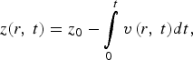 $$z\lpar r\comma \; t\rpar =z_0 - \vint\limits_0^t {v\left({r\comma \; t} \right)} dt\comma \;$$
where z 0 is the original position of the surface at the beginning of the calculation (i.e., disruption or off-normal event) and v(r,t) is the surface velocity. Using the fact that in our problem, symmetry exists so that we can consider ∂T /∂r = 0 the equation transforms into:
 $${\rm \rho} c_p \displaystyle{\partial T \over \partial t} = {\rm \rho} \left(T \right)cp \left(T \right)V\left(r\comma \; t \right)\displaystyle{\partial T \over \partial z} + \mathop{q}\limits^{\bullet} \left(r\comma \; z\comma \; t \right)\comma \;$$
that includes a convective term before not present. The boundary condition seen before applies for z = 0. Typically the temperature at the boundary inside the material is given for two dimensions but it is fixed and equal to the ambient temperature T b. The surface velocity needed to evaluate the boundary condition can be calculated from (Hassanein, Reference Hassanein1984):
 $$V\lpar r\comma \; t\rpar = 5.8 \bullet 10^{ - 2} \displaystyle{{\rm \alpha} \sqrt{A} P_V \left(T_V \right)\over {\rm \rho} \left(T_V \right)\sqrt{T_V}} \bullet \left[0.8 + 0.2e^{\displaystyle{ - t \over 10{\rm \tau}_C}} \right]\comma \;$$
where α is the sticking probability, A is the atomic mass of the target material, P V is the vapor pressure, and τC is the collision time.
2.2. Plasma: Vapor Interaction
Once the material under heat flux load starts vaporizing, the screening effect of the cloud directly onto the target material becomes more and more efficient. As enough energy reaches the area, ionized vapor will start forming and interacting with the inclined magnetic field that will limit the expansion of the vapor itself. The ions will only move along the magnetic lines. In this condition, further heating of the surface is due only to vapor thermal radiation and thermal conduction. The expansion of the vapor into vacuum is then determined by solving the MHD equations for conservation of mass, momentum and energy (Hassanein & Konkashbaev, Reference Hassanein and Konkashbaev1994):
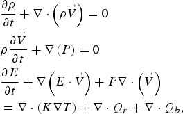 $$\eqalign{&\displaystyle{\partial {\rm \rho} \over \partial t} + \nabla \cdot \left({\rm \rho} \vec{V} \right)= 0 \cr &{\rm \rho} \displaystyle{\partial \vec{V} \over \partial t} + \nabla \left(P \right)= 0 \cr &\displaystyle{\partial E \over \partial t} + \nabla \left(E \cdot \vec{V} \right)+P\nabla \cdot \left(\vec{V} \right)\cr &= \nabla \cdot \left(K\nabla T \right)+ \nabla \cdot Q_r + \nabla \cdot Q_b\comma \; }$$
where ρ is the density,  $\vec{V}$ is the vapor velocity, P is the pressure, E is the energy, K is the vapor conductivity, Q b is the incident particle flux from the incoming plasma, and Q r is the radiation flux. The vapor plasma once it is ionized moves freely along the inclined magnetic field lines. The equation describing the vapor motion in a magnetic field is given by (Hassanein & Konkashbaev, Reference Hassanein and Konkashbaev1994):
 $${\rm \rho} \displaystyle{\partial \vec{V} \over \partial t} = - \nabla P + \vec{J} \times \vec{B}.$$
The magnetic force  $\vec{J} \times \vec{B}$ acts as a retarding force for the expanding vapor with important consequences toward the final and total erosion of the plate. The perpendicular component to the B field of the force is predominant. Two parts compose the magnetic force: F magnetic or magnetic pressure force and F curvature due to the curvature of the magnetic field:
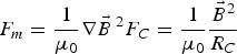 $$F_m = \displaystyle{1 \over {\rm \mu}_0} \nabla \vec{B}\,^2F_C = \displaystyle{1 \over {\rm \mu}_0} \displaystyle{\vec{B}^2 \over R_C}$$
The current density is given by:
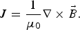 $$J = \displaystyle{1 \over {\rm \mu}_0} \nabla \times\vec{B}.$$
The magnetic diffusion in the vapor cloud needs to be considered in the solution of the MHD equation. The variation along time of the magnetic field can be calculated with:
 $$\displaystyle{\partial B \over \partial t} = - \displaystyle{1 \over {\rm \mu}_0} \nabla \times \left({\rm \varepsilon} + \vec{V} \times \vec{B} \right)\comma \;$$
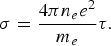
where ε is the induced electric field and can be calculated as  ${\rm \varepsilon} = \vec{J}/{\rm \sigma}$. The vapor conductivity σ for weakly ionized plasma is directly proportional to the vapor plasma collision time τ and density ne and inversely proportional to the mass of the electron:
 $${\rm \sigma} = \displaystyle{4{\rm \pi} n_e e^2 \over m_e} {\rm \tau}.$$
The vapor equations are solved in two-dimensional coordinates (X axis and Y axis) system along and across the magnetic field lines (Fig. 2). Z-axis is the toroidal axis while Y-axis is the poloidal one.
(Color online) Schematic illustration of HEIGHTS-PIC geometry and axes.
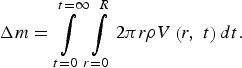
then they are transformed back to the xy axis reference (perpendicular to the target plate and parallel to the divertor). Joule heating of the vapor cloud is also considered and evaluated in this phase of the calculation. In order to evaluate the eroded mass due to the disruption on the reference target surface, the following relationship is used:
 $$\Delta m = \vint\limits_{t = 0}^{t = \infty} \vint\limits_{r = 0}^R 2{\rm \pi} r{\rm \rho} V\left(r\comma \; t \right)dt.$$
From the mass, using the density of the material, the thickness or depth of the eroded material can be calculated.
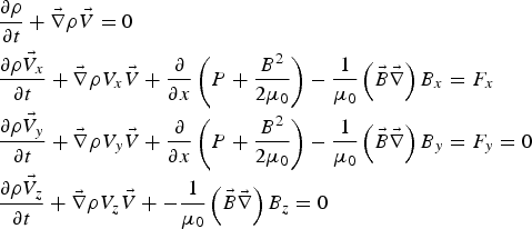
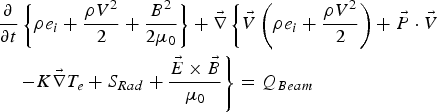
The entire system of magneto-hydro-dynamics equations can be summarized as (18) for mass continuity and momentum continuity equation, (19) for energy conservation and (20) for Maxwell equations:
 $$\eqalign{&\displaystyle{\partial {\rm \rho} \over \partial t} + \vec{\nabla} {\rm \rho} \vec{V} = 0 \cr &\displaystyle{\partial {\rm \rho} \vec{V}_x \over \partial t} + \vec{\nabla} {\rm \rho} V_x \vec{V} + \displaystyle{\partial \over \partial x} \left(P + \displaystyle{B^2 \over 2{\rm \mu}_0} \right)- \displaystyle{1 \over {\rm \mu}_0} \left(\vec{B} \vec{\nabla} \right)B_x = F_x \cr &\displaystyle{\partial {\rm \rho} \vec{V}_y \over \partial t} + \vec{\nabla} {\rm \rho} V_y \vec{V} + \displaystyle{\partial \over \partial x} \left(P + \displaystyle{B^2 \over 2{\rm \mu}_0} \right)- \displaystyle{1 \over {\rm \mu}_0} \left(\vec{B} \vec{\nabla} \right)B_y = F_y = 0 \cr &\displaystyle{\partial {\rm \rho} \vec{V}_z \over \partial t}+ \vec{\nabla} {\rm \rho} V_z \vec{V} + - \displaystyle{1 \over {\rm \mu}_0} \left(\vec{B} \vec{\nabla} \right)B_z = 0}$$
 $$\eqalign{&\displaystyle{\partial \over \partial t} \left\{{\rm \rho} e_i + \displaystyle{{\rm \rho} V^2 \over 2} + \displaystyle{B^2 \over 2{\rm \mu}_0} \right\}+ \vec{\nabla} \left\{\vec{V} \left({\rm \rho} e_i + \displaystyle{{\rm \rho} V^2 \over 2} \right)+ \vec{P} \cdot \vec{V} \right. \cr &\left. \quad - K \vec{\nabla} T_e + S_{Rad} + \displaystyle{\vec{E} \times \vec{B} \over {\rm \mu}_0} \right\}= Q_{Beam}}$$
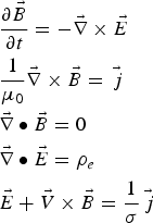 $$\eqalign{&\displaystyle{\partial \vec{B} \over \partial t} =- \vec{\nabla} \times \vec{E} \cr &\displaystyle{1 \over {\rm \mu}_0} \vec{\nabla} \times \vec{B} = \vec{\,j} \cr &\vec{\nabla} \bullet \vec{B} = 0 \cr &\vec{\nabla} \bullet \vec{E}={\rm \rho} _e \cr &\vec{E}+\vec{V} \times \vec{B} = \displaystyle{1 \over {\rm \sigma} }\vec{\,j}}$$
where T e is the target plasma electron temperature, σ is the plasma conductivity, and  $\vec{\,j} $ is the electric current density. Also,
 $\vec{B}$ is the magnetic field inductance,
 ${\rm \rho}\comma \; \vec{V}\comma \; e_i\comma \; P$ are the plasma density, the velocity, thermal energy, and the pressure while Srad is the radiation heat flux. No viscosity term is considered given the high heating due to the incoming hot plasma. Q is the power density deposited to the target plasma and the target by the incoming hot SOL plasma by collisional stopping. If the Poynting vector term
 $\vec{\nabla} {\vec{E}{\rm \times} \vec{B} \over {\rm \mu}_0}$ and the equation of the magnetic field are rewritten using Ohm's law and Maxwell's equation, the system of equations can be transformed and rewritten with analogy to (18)–(20) into (Hassanein & Konkashbaev, Reference Hassanein and Konkashbaev1994):
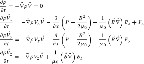 $$\eqalign{&\displaystyle{\partial {\rm \rho} \over \partial t} = - \vec{\nabla} {\rm \rho} \vec{V} = 0 \cr &\displaystyle{\partial {\rm \rho} \vec{V}_x \over \partial t} = - \vec{\nabla} {\rm \rho} V_x \vec{V} - \displaystyle{\partial \over \partial x}\left(P + \displaystyle{B^2 \over 2{\rm \mu}_0} \right)+ \displaystyle{1 \over {\rm \mu}_0} \left(\vec{B} \vec{\nabla} \right)B_x + F_x \cr &\displaystyle{\partial {\rm \rho} \vec{V}_y \over \partial t} = - \vec{\nabla} {\rm \rho} V_y \vec{V} - \displaystyle{\partial \over \partial x} \left(P + \displaystyle{B^2 \over 2{\rm \mu}_0} \right)+ \displaystyle{1 \over {\rm \mu}_0} \left(\vec{B} \vec{\nabla} \right)B_y \cr &\displaystyle{\partial {\rm \rho} \vec{V}_z \over \partial t} = - \vec{\nabla} {\rm \rho} V_z \vec{V} + \displaystyle{1 \over {\rm \mu}_0} \left(\vec{B} \vec{\nabla} \right)B_z}$$
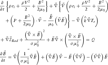 $$\eqalign{&\displaystyle{\partial \over \partial t} \left\{{\rm \rho} e_i + \displaystyle{{\rm \rho} V^2 \over 2} + \displaystyle{B^2 \over 2{\rm \mu}_0} \right\}+ \vec{\nabla} \left\{\vec{V} \left({\rm \rho} e_i + \displaystyle{{\rm \rho} V^2 \over 2} + \displaystyle{B^2 \over 2{\rm \mu}_0} \right)\right. \cr &\quad \left. + \left(P + \displaystyle{B^2 \over 2{\rm \mu}_0} \right)\cdot \vec{V} - \displaystyle{\vec{B} \over {\rm \mu}_0} \left(\vec{V} \vec{B} \right)\right\}- \vec{\nabla} \left(\mathop{k}\limits^{\wedge} \vec{\nabla} T_e \right) \cr &+ \vec{\nabla} \vec{S}_{Rad} + \displaystyle{\left(\vec{\nabla} \times \vec{B} \right)^2 \over {\rm \sigma} {\rm \mu}_0^2} + \vec{B} \vec{\nabla} \times \left(\displaystyle{\vec{\nabla} \times \vec{B} \over {\rm \sigma} {\rm \mu}_0^2} \right)= Q \cr &\displaystyle{\partial \vec{B} \over \partial t} = \vec{\nabla} \vec{\left(\displaystyle{1 \over {\rm \sigma} {\rm \mu}_0^2} \vec{\nabla} \vec{B} \right)} + \left(\vec{\nabla} \vec{B} \right)\vec{V} - \vec{B} \left(\vec{\nabla} \vec{V} \right)- \left(\vec{V} \vec{\nabla} \right)\vec{B}}$$
In the last equation, it is clear that the first term on the right-hand side describes the diffusion while the second describes the convection of the magnetic field. Along the three main axes, the last equation can be written as:
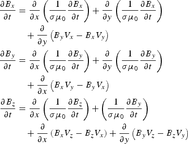 $$\eqalign{\displaystyle{\partial B_x \over \partial t} &= \displaystyle{\partial \over \partial x} \left(\displaystyle{1 \over {\rm \sigma} {\rm \mu}_0} \displaystyle{\partial B_x \over \partial t} \right)+ \displaystyle{\partial \over \partial y} \left(\displaystyle{1 \over {\rm \sigma} {\rm \mu}_0} \displaystyle{\partial B_x \over \partial t} \right)\cr &\quad + \displaystyle{\partial \over \partial y} \left(B_y V_x - B_x V_y \right)\cr \displaystyle{\partial B_y \over \partial t} &= \displaystyle{\partial \over \partial x} \left(\displaystyle{1 \over {\rm \sigma} {\rm \mu}_0} \displaystyle{\partial B_y \over \partial t} \right)+ \displaystyle{\partial \over \partial y} \left(\displaystyle{1 \over {\rm \sigma} {\rm \mu}_0} \displaystyle{\partial B_y \over \partial t} \right)\cr &\quad + \displaystyle{\partial \over \partial x} \left(B_x V_y - B_y V_x \right)\cr \displaystyle{\partial B_z \over \partial t} &= \displaystyle{\partial \over \partial x} \left(\displaystyle{1 \over {\rm \sigma} {\rm \mu}_0} \displaystyle{\partial B_z \over \partial t} \right)+ \left(\displaystyle{1 \over {\rm \sigma} {\rm \mu}_0} \displaystyle{\partial B_y \over \partial t} \right)\cr &\quad + \displaystyle{\partial \over \partial x} \left(B_x V_z - B_z V_x \right)+ \displaystyle{\partial \over \partial y} \left(B_y V_z - B_z V_y \right)}$$
In the solution of the systems of equations, very important are the boundary conditions imposed to the computational domain. In particular, they need to be imposed on all four sides of the domain with special consideration to the treatment of the heat transport inside the solid target. It is assumed that the target is a bulk material so that a reflective boundary condition is imposed with the addition of a source due to vaporization. For the “side walls” (still considered as computational domain since the only effective and real wall is the target itself), reflective boundary conditions are chosen. This means that the plasma expansion is stopped at rigid walls or at the boundary. The artificial mesh created around the computational domain to impose the boundary condition can then be determined assigning to those cells precise values. The momentum perpendicular to the boundary cells has generally opposite sign with respect to the neighboring meshes. All the other values (as temperature, pressure, density, or mass associated to the cell) are kept identical to the fist mesh while energy is imposed equal to zero. The value of B x is not assumed to be frozen at the graphite target and posed equal to the one in the first computational cell: this is done to evaluate eventual diamagnetic effects.
2.3. Radiation Transport and Optical Properties of Plasma
After enough vapors has accumulated in front of the divertor plate, the impinging plasma particles will be totally stopped by the vapor cloud with residual heating and ionization of the cloud itself. Photon radiation by the vapor cloud is then emitted due to the continuous vapor heating process. At this point plasma energy is transmitted to the divertor/target surface only indirectly through photon radiation determining the final erosion rate. Radiation is composed by two different fluxes: continuum radiation and line radiation. Given the highly dynamical development of the disruption/instability process, the radiation process cannot be considered stationary so that the radiation transport equation should be written as (Hassanein & Konkashbaev, Reference Hassanein and Konkashbaev1994):
 $$\left[\displaystyle{1 \over c} \displaystyle{\partial \over \partial t} + \vec{\Omega} \bullet \nabla \right]I_{{\rm \upsilon}} = {\rm \eta}_{{\rm \upsilon}} - {\rm \alpha}_{{\rm \upsilon}} I_{{\rm \upsilon}}\comma \;$$
where I ν is the radiation intensity, ν is the frequency, ην is the vapor emissivity,  $\vec{\Omega}$ is the solid angle, and αν is the absorption coefficient. Based on the carbon available atomic data, the collisional-radiation (CRE) equilibrium model is used to calculate the ion population balance of the plasma, thermodynamic functions, and above all the absorption and emission coefficient at each time step. Collisional processes include collisional excitation and re-excitation, collisional ionization and three-body recombination. The populations of atomic levels are determined from detailed analysis of collisional and radiative atomic processes. The latter ones can include discrete spontaneous transitions, photo recombination, and dielectric recombination. In collisional process, free electrons transfer energy to bound electrons (excitation and ionization) while in a pure radiative process, photons transfer all their energy to electrons via inverse Bremsstrahlung radiation, photo-excitation and photoionization. Collisional de-excitation, recombination, radiative de-excitation, spontaneous and induced emission, bremsstrahlung and dielectric recombination are all inverse processes.
Using the level populations, the emission and absorption coefficients are calculated evaluating the transition probabilities between the various energetic states. Transitions taken into account are the free-free, bound-free, and bound-bound type. This last transition produces an emission or absorption of line radiation.
For values of plasma densities above 1018 cm−3 and relative low temperatures (less than 10 eV), plasma can be considered in local thermodynamic equilibrium (LTE). In such conditions, plasma is dominated by recombination and de-excitation processes: Saha equation is used for the calculation of ions concentration, while both emission and absorption coefficients are considered identical. The level populations are calculated using Boltzmann distribution.
For values of plasma densities below 1017 cm−3 and temperatures larger than 10 eV, the LTE approximation cannot be considered valid since recombination, dielectric recombination and radiative de-excitation become much more important and cannot be considered negligible anymore. Non-LTE plasmas exhibit typically a lower ionization degree as well as a population of exited levels. For such reasons the emission coefficients of non-LTE plasmas are smaller.
In optically thin plasmas, the transitions frequencies of all atomic processes are dependent solely on density and temperature. For this reason, radiative excitation and ionization processes have a negligible influence. In optically thick plasmas, reabsorption of radiation is occurring. Radiative excitation and ionization have to be calculated as well as their transition probabilities. Both these quantities depend on the local radiation flux, which is typically obtained from the transport calculations. In this case calculations are performed for plasma with constant density and temperature.
Hydrodynamic equations are written in form of pressure and internal energy and coupled with the radiation transport equations written as functions of the density and temperature. The two processes are solved self-consistently into HEIGHTS-PIC while the equation of state for carbon represents the link between these two processes. The radiation transport solutions also use additional information regarding the ionic and electronic concentrations in the plasma which depend on the populations of atomic levels and charge distribution in each examined cell of the mesh.
To solve the radiation transport along each time step, the absorption and emission coefficients are calculated for each cell. They depend on temperature, density, ionization state and are also functions of the frequency of absorbed and emitted elements. The calculation is very complex since for each computational cell and for each time step, the populations' levels and cross-sections of the atomic processes must be evaluated making this part of the calculation particularly intensive. For getting highly accurate results, the populations of atomic levels and ion structure of the plasma are also calculated.
The use of the tabulated values for the energy levels, oscillator strength and other atomic parameters allows the calculation of photoionization cross-sections or the constants to evaluate the radiation broadening of spectral lines. The ionization structure of the plasma and populations of atomic levels can be found using the non-steady kinetic equation (Hassanein & Konkashbaev, Reference Hassanein and Konkashbaev1994):
 $$\displaystyle{dN_i \over dt} = - N_i \sum\limits_{\,j \ne i} K_{i\comma j} + \sum\limits_{i \ne j} N_j K_{\,j\comma i}\comma \;$$
where N i is the population of atomic levels i produced by the transitions from this level to other level j (with transition rate equal to K i,j ) and the transitions from other level j to the level i (with transition rate equal to K j,i this time). If the ground level is i, then this is the ion concentration in the plasma.
To be complete, one equation for each atomic level needs to be written. If atomic transitions are much faster than the typical thermodynamic processes of the plasma, then the atomic system can be considered in equilibrium for each hydrodynamic step so that the previous equation becomes homogeneous:
 $$0 = - N_i \sum\limits_{\,j \ne i} K_{i\comma j} + \sum\limits_{i \ne j} N_j K_{\,j\comma i}\comma \;$$
so that
 $$\displaystyle{dN_i \over dt} = 0.$$
Since the kinetic rates of radiation and photoionization strictly depend on the radiation flux, the equations just seen need to be integrated with frequency-dependent equations of radiation transport which are defined by the radiation process in the whole plasma domain. The problem is then spatially non-local. The CRE approximation accounts for collisional processes, photo de-excitation and photo-recombination while it neglects the processes of photo-excitation and photo-ionization. This means that locally the approximation well describes the characteristics of optically thin plasmas in a wide range of temperature and density as it happens in our simulations.
Using this approximation, excited states are connected only with the ground state so that only collisional excitation and radiation de-excitation are considered. These effects are present in very hot, optically thick plasmas. Collisional transitions as well as radiative decay from higher bound levels are considered united with three-body recombination and radiative recombination. This methodology is complicated and computationally intensive: for this reason it is very important to choose wisely both the number of sample particles representing the plasma as well as the proper size of computational grid.
Transition rates K i,j are defined by the interplay of radiative and collisional processes. Different transitions are described by different processes: the transition to continuum spectrum is defined by the electronic collisional ionization while the discrete transitions from lower level to higher levels are described by the electronic collisional excitation.
The rate of transitions to the lower level can be obtained from the radiative spontaneous transitions and electronic collisional de-excitation. The recombination rate is calculated taking into account dielectronic recombination, three-body recombination and photo-recombination. The first one in particular, is determined by the ion capture of an electron and concurrent excitation of the associated electron. This leads to a spontaneous transition to the ground state. Also in the calculation for the ionization and excitation rates the radiative processes of photo-excitation and photoionization need to be considered. This complicates the sets of equation since the processes are generally defined by non-local plasma properties making the solution of the algorithm quite complex and needing inputs from the solutions of the hydrodynamic part.
For calculating the opacities of the plasma acting on the entire computational mesh, it is important to evaluate all three contributions coming from the Bremsstrahlung radiation, the photo-ionization from the ground, excited and inner cells, and finally the discrete transitions. Each effect is described by the corresponding cross section. The profiles of spectral lines need special attention since all broadening mechanisms (Doppler, Stark and radiation) might be important according to the conditions of the plasma. Stark broadening though plays a dominant role among those and in our simulations.
The total absorption coefficient k tot depends on local values of density ρ, the temperature T and the ionization Z of the plasma. The absorption coefficients can be written as:
 $$\eqalign{k_{tot} \left({\rm \rho}\comma \; T\comma \; h{\rm \upsilon} \right)&= k_{\,free \;free}\left({\rm \rho}\comma \; T\comma \; h{\rm \upsilon} \right)+ k_{bound \;free} \left({\rm \rho}\comma \; T\comma \; h{\rm \upsilon} \right)\cr &\quad + k_{bound \;bound} \left({\rm \rho}\comma \; T\comma \; h{\rm \upsilon} \right).}$$
The total value then is calculated summing up the contribution from each free-free transition, bound-free and bound-bound transitions with i and j the energy states, j is the excitation level while i is the ionization state. The single contributions are defined as:
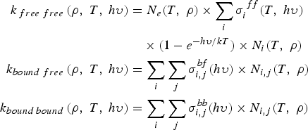 $$\eqalign{k_{\,free \;free} \left({\rm \rho}\comma \; T\comma \; h{\rm \upsilon} \right)&= N_e \lpar T\comma \; {\rm \rho} \rpar \times \sum\limits_i {\rm \sigma}_i^{\,ff} \lpar T\comma \; h{\rm \upsilon} \rpar \cr &\quad \times \lpar 1 - e^{ - h{\rm \upsilon} /kT}\rpar \times N_i \lpar T\comma \; {\rm \rho} \rpar \cr k_{bound \;free}\left({\rm \rho}\comma \; T\comma \; h{\rm \upsilon} \right)&= \sum\limits_i \sum\limits_j {\rm \sigma}_{i\comma j}^{bf} \lpar h{\rm \upsilon}\rpar \times N_{i\comma j} \lpar T\comma \; {\rm \rho}\rpar \cr k_{bound \;bound}\left({\rm \rho}\comma \; T\comma \; h{\rm \upsilon} \right)&= \sum\limits_i \sum\limits_j {\rm \sigma}_{i\comma j}^{bb} \lpar h{\rm \upsilon}\rpar \times N_{i\comma j} \lpar T\comma \; {\rm \rho}\rpar}$$
Line radiation and profiles need accurate evaluation. Atomic and ionic spectral lines originate from specified electronic transitions between very well defined energy levels of atoms and ions. The lines though are not sharp because of several broadening mechanics so that the effective line has a finite width which must be calculated or approximated. The mechanisms that contribute to the finite width of the line profile are four: natural broadening, Doppler broadening, Stark broadening and interaction with neighboring particles.
The broadening of the Stark effect can be significant with respect to the natural one. In highly ionized and moderately dense plasmas, Stark broadening is definitely the dominant effect and becomes more and more effective as temperature and density rise. In fact the energy levels within a single atom may be modified due to the electric field of nearby atoms or ions.
The CRE model used in HEIGHTS-PIC well describes the optically thin steady state plasma. However, in presence of optically thick plasma or external energy applied, the CRE model needs modifications so that the model becomes self-consistent and non-local. Additional effects are added in our case and they generally depend on the initial state of the problem. In particular, the photoionization process is particularly important in the description of plasmas with high temperature gradients. In the solution of the radiation transport equation, the computational mesh used for its solution not necessarily coincides with the one used to solve the hydrodynamic solution. In fact, the two systems are decoupled, and the radiation transport can be solved using a different grid. In the simulations here proposed, the radiation transport is solved using a quadrangular mesh (versus the hydrodynamic one which is rectangular) formed by 6 cells by 6 cells or 12 by 12 cells and so on: those cells are then bigger than the ones used into the hydrodynamic solution. This allows more flexibility as well as the possibility to choose the best configuration according to the aimed accuracy. The solid angle is subdivided in eight main rays (Fig. 3).
(Color online) Schematic illustration of ray tracing methods and cylindrical radiation basic geometry in HEIGHTS-PIC.
The transport of energy is calculated precisely along this geometrical configuration covering well both isotropic and anisotropic behaviors. In fact, the photon propagation wave nature can be well represented by cylindrical coordinates. So while as described before, the hydrodynamic part of the PIC solution is well described by a rectangular domain, the radiation transport solution uses cylindrical coordinates to solve the radiation transport equation. A specific subroutine into HEIGHTS-PIC takes care for each time step of the mapping from the rectangular grid to the cylindrical and vice versa. In Figure 3 it can be seen the relationship between the hydrodynamic PIC cells established in the Eulerian mesh and the smaller in number cylindrical radiation transport cells chosen by the division into sectors. So many hydrodynamics cells can be included in one cylindrical radiative one. With the use of this methodology, photon-deposited energy can be tracked with great accuracy allowing improved accuracy in the solutions of the problem.
For continuum radiation the set of self-consistent equations are given by (Hassanein & Konkashbaev, Reference Hassanein and Konkashbaev1994):
 $$\displaystyle{1 \over c}\displaystyle{\partial I_{{\rm \upsilon}} \over \partial t} + \vec{\Omega} \bullet \nabla I_{{\rm \upsilon}} = - \left({\rm \alpha}_{{\rm \upsilon}} I_{{\rm \upsilon}} - {\rm \eta}_{{\rm \upsilon}} \right)= - {\rm \alpha}_{{\rm \upsilon}} \left(I_{{\rm \upsilon}} - S_{{\rm \upsilon}} \right)\comma \;$$
associated with the material energy equation :
 $$\displaystyle{\partial E \over \partial t} = 4{\rm \pi} \vint {\rm \alpha}_{{\rm \upsilon}} \left(J_{{\rm \upsilon}} - S_{{\rm \upsilon}} \right)d {\rm \upsilon} + Q\comma \;$$
where as before, I í is the radiation intensity, í is the frequency, ç í is the vapor emissivity,  $\vec{\Omega}$ is the solid angle, and á í is the absorption coefficient, Q represents other energy sources and J í is the angle-averaged radiation intensity:
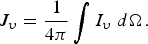 $$J_{{\rm \upsilon}} =\displaystyle{1 \over 4{\rm \pi}} \vint I_{{\rm \upsilon}} \;d \Omega.$$
And S ν = ην/αν is the source function. In LTE, the source function is the Plank function B ν and depends only on temperature.
Discretizing in time and linearizing about the actual temperature T 0, the material energy equation reads:
 $$c_T \left(T - T_0 \right)= \Delta t\vint {\rm \alpha}_{{\rm \upsilon}} \left(J_{{\rm \upsilon}} - S^0_{{\rm \upsilon}} \right)d {\rm \upsilon} + Q\Delta t\comma \;$$
where c T is the specific heat for the total system of matter and radiation. Combining this equation with the linearized version of the transport, it follows (Buneman, Reference Buneman1959):
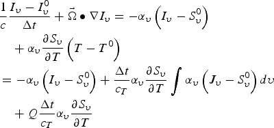 $$\eqalign{&\displaystyle{1 \over c} \displaystyle{I_{{\rm \upsilon}} - I^0_{{\rm \upsilon}} \over \Delta t} +\vec{\Omega} \bullet \nabla I_{{\rm \upsilon}} =- {\rm \alpha}_{{\rm \upsilon}} \left(I_{{\rm \upsilon}} - S^0_{{\rm \upsilon}} \right)\cr &\quad + {\rm \alpha}_{{\rm \upsilon}} \displaystyle{\partial S_{{\rm \upsilon}} \over \partial T} \left(T - T^0 \right) \cr &=- {\rm \alpha}_{{\rm \upsilon}} \left(I_{{\rm \upsilon}} - S^0_{{\rm \upsilon}} \right)+ \displaystyle{\Delta t \over c_T} {\rm \alpha}_{{\rm \upsilon}} \displaystyle{\partial S_{{\rm \upsilon}} \over \partial T} \vint {\rm \alpha}_{{\rm \upsilon}} \left(J_{{\rm \upsilon}} - S^0_{{\rm \upsilon}} \right)d {\rm \upsilon} \cr &\quad + Q \displaystyle{\Delta t \over c_T} {\rm \alpha}_{{\rm \upsilon}} \displaystyle{\partial S_{{\rm \upsilon}} \over \partial T}}$$
In this equation, the integral term couples together intensities for all frequencies and for all angles. In our case, the entire space is divided into eight fundamental directions or rays and the equation, solved for each single one, accounts for a portion of the real diffusion and movement of the radiation field.
For line radiation the set of self-consistent equations are instead given by:
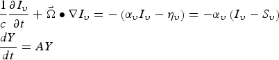 $$\eqalign{&\displaystyle{1 \over c}\displaystyle{\partial I_{{\rm \upsilon}} \over \partial t} + \vec{\Omega} \bullet \nabla I_{{\rm \upsilon}} =- \left({\rm \alpha}_{{\rm \upsilon}} I_{{\rm \upsilon}} - {\rm \eta}_{{\rm \upsilon}} \right)= - {\rm \alpha}_{{\rm \upsilon}} \left(I_{{\rm \upsilon}} - S_{{\rm \upsilon}} \right)\cr &\displaystyle{dY \over dt} =AY}$$
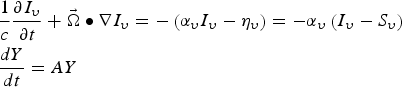 $$\eqalign{&\displaystyle{1 \over c} \displaystyle{\partial I_{{\rm \upsilon}} \over \partial t} + \vec{\Omega} \bullet \nabla I_{{\rm \upsilon}} =- \left({\rm \alpha}_{{\rm \upsilon}} I_{{\rm \upsilon}} - {\rm \eta}_{{\rm \upsilon}} \right)= - {\rm \alpha}_{{\rm \upsilon}} \left(I_{{\rm \upsilon}} - S_{{\rm \upsilon}} \right)\cr &\displaystyle{dY \over dt} =AY}$$
where Y is the vector representing the population densities of the atomic levels and A is the rate matrix.
The total rate A ij connecting two generic atomic levels i and j, includes all collisional and radiative transitions both discrete (bound-bound) and continuous (free-bound). The different populations respond to radiation through the effects on the transition rates. Both absorption and emission coefficients are calculated similarly to the procedure explained in Morozov et al. (Reference Morozov, Tolkach and Hassanein2004).
3. TARGET PLATE GEOMETRY AND COMPUTATIONAL SETUP
The first one (X-axis, Fig. 3) is perpendicular to the divertor plate and it will provide a spatial measure of the evolution of the plasma above the target. The Y-axis is the radial direction of the toroid and is also the “poloidal direction” for the B field. The Z-axis instead represents the toroidal direction for the B field. The computational grid (Fig. 4) where the mesh will be placed is so perpendicular to the plate and provides a spatial projection of the plasma movement along time (Genco & Hassanein, Reference Genco and Hassanein2011. The mesh is formed by rectangular cells having X and Y components. The number of cells along X and Y can be chosen arbitrarily, as well as the inclination of the divertor plate with respect to the natural axis X nat and Y nat (Fig. 5). The toroidal angle (or magnetic angle) can also be chosen and it is the angle between the B field and the divertor plate.
(Color online) Schematic illustration of HEIGHTS-PIC geometry with carbon plasma super particles formation.
(Color online) Schematic illustration of HEIGHTS-PIC geometry and axes with angle over Y nat.
The initial state of the computational mesh is defined having some cells (the ones directly facing the divertor or target plate) filled with neutral vapor with a specified initial density. Some important assumptions regard the absence of motion along the Y-axis as the fact that the beam energy is deposited and absorbed according to the range of ions. The plasma disruption is then numerically “interpreted” as a beam of energy with specified characteristics as the shape, flux, and maximum intensity. In particular HEIGHTS-PIC supports so far three fundamental beam shapes as the uniform one, the Gaussian one and the exponential one with peak close to the striking point on the divertor.
One of the boundaries (the target plate) has a dynamical evolution and allows for the introduction of new generated sample particles as the material melts and vaporizes. A fixed grid is used for the Eulerian frame while an adapted one is used in to the Lagrangian phase. The nonlinear convection term associated with the Eulerian formulation does not appear when transitional effects are not considered and when the density is frozen at this stage. The motion of the system is analyzed into the Lagrangian step and final phase leaving the interior state unchanged. The sample particles or “super particles” are considered one-dimensional allowing them to be stacked along the Y-axis and in layers along the X-axis but having no dimension in this direction (Fig. 4). The disruption modeling includes the interaction with the plate solid target, vaporized gas, and divertor plasma in magnetic field configuration. No map is used to transfer the properties from particles to the original grid as the conditions established by the ensemble of particles in a cell are evaluated producing the same effect inside the cell itself. In order to start the hydrodynamic computational part, a neutral vapor (loaded with some sample particles) is supposed to be close to the target at the time the energy impact starts. The evolving characteristics of the particles inside the cells are assumed homogeneous throughout the cells.
Diffusion due to the presence of the B field is also considered and incorporated into the particle motion with possibility to set different starting diffusion coefficients.
Several blocks constitute the HEIGHTS-PIC package including heat conduction, divertor surface vaporization and particle generation, plasma material interaction and MHD models. The MHD block (Eulerian and Lagrangian part) integrates the plasma hydrodynamic evolution, magnetic diffusion, heat conduction, and radiation transport.
Starting from the continuity equations of mass, momentum and energy coupled with the equation of state and the definition of internal energy, three steps can be identified. The first one (Eulerian step) considerers the variation of the internal state of a subsystem (N particles) followed by the analysis of the motion of the subsystem leaving the internal state unchanged (Lagrangian and final step). Let's now examine one by one the single steps.
In the Eulerian step, considering the rectangular computational domain above described, only quantities of the cells as whole are changed. The plasma-vapor fluid is assumed to be constraint, translational effects dropped from the equations (convective terms as div(ρV) or div(ρEV) equal to zero) so that density can be considered “frozen” and taken out from the differentiation reducing the equations to:
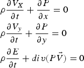 $$\eqalign{&{\rm \rho} \displaystyle{\partial V_X \over \partial t} + \displaystyle{\partial P \over \partial x} = 0 \cr &{\rm \rho} \displaystyle{\partial V_y \over \partial t} + \displaystyle{\partial P \over \partial y} = 0 \cr &{\rm \rho} \displaystyle{\partial E \over \partial t} + div\lpar P\vec{V}\rpar = 0}$$
Using centered finite difference approximation with central difference the expressions can be written as follows assuming the velocity components along X-axis as u and Y-axis as v;  $\tilde{u}\comma \; \tilde{v}\comma \; \tilde{E}$ are intermediate values obtained assuming that the density ρ is “frozen” or unchanged along the time t n + Δt. Even if the Eulerian scheme in such way may result in some numerical instability, the entire scheme with the Lagrangian and final step is stable. Of critical importance will be the choice of the time step chosen well below the classical Courant condition (Courant et al., Reference Courant, Friedrichs and Lewy1928).
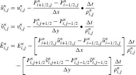 $$\eqalign{\tilde{u}_{i\comma j}^n &= u_{i\comma j}^n - \displaystyle{P_{i+1/2\comma j}^n - P_{i - 1/2\comma j}^n \over \Delta x} \bullet \displaystyle{\Delta t \over {\rm \rho} _{i\comma j}^n} \cr \tilde{v}_{i\comma j}^n &= v_{i\comma j}^n - \displaystyle{P_{i\comma j+1/2}^n - P_{i\comma j - 1/2}^n \over \Delta y} \bullet \displaystyle{\Delta t \over {\rm \rho}_{i\comma j}^n} \cr \tilde{E}_{i\comma j}^n &= E_{i\comma j}^n - \left[\displaystyle{P_{i + 1/2\comma j}^n \tilde{u}_{i + 1/2\comma j}^n - P_{i - 1/2\comma j}^n \tilde{u}_{i - 1/2\comma j}^n \over \Delta x} \right]\displaystyle{\Delta t \over {\rm \rho}_{i\comma j}^n} \cr &\quad - \left[\displaystyle{P_{i\comma j + 1/2}^n \tilde{v}_{i\comma j + 1/2}^n - P_{i\comma j - 1/2}^n \tilde{v}_{i\comma j - 1/2}^n \over \Delta y} \right]\displaystyle{\Delta t \over {\rm \rho} _{i\comma j}^n}}$$
Quantities with fractional subscripts are related to cell boundaries using the following formulation:
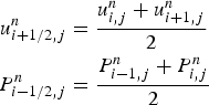 $$\eqalign{u_{i + 1/2\comma j}^n &= \displaystyle{u_{i\comma j}^n + u_{i + 1\comma j}^n \over 2} \cr P_{i - 1/2\comma j}^n &= \displaystyle{P_{i - 1\comma j}^n + P_{i\comma j}^n \over 2}}$$
For each step, particles in the cells are stacked following the original set up division decided at the beginning. In the simulations here presented, each cell is subdivided along Y-axis in five divisions and in each of those internal subdivisions, particles are stacked as needed. No real dimension is considered along the X-axis. The cells can be then considered layered even though particles do not respect any physical effective dimension and do not produce local violation of conservation laws. The values of the “layers” along the X direction change per each cell of the mesh dynamically along time and due to for motion, forces and the eventual new production of new particles. Whenever the mass of vapor exceeds a pre-established value, a new super particle is produced. This pre-established value of mass can be changed defining the results more accurately according to how much mass a single super particle represents. Also the system is “constantly fed” through the melting and evaporating boundary at the target plate while particles reaching the left or right side of the computational domain might be “lost” by the system. Also, in the computational solution, for the upper boundary, only cells effectively “filled” in with particles are calculated speeding up the calculation.
In the Lagrangian step once particles have been eventually produced and allocated into the closest cells according to their birth origin, they are ordered according to the particle mover. The position of the vapor front along X-axis and Y-axis and for each cell is compared with the original mesh and this provides the new position of the particles in the cells. Eventually, if the front did not move outside the cell borders, the number of particles in the cells is increased. At this point, the new momentum fluxes are calculated as well as the new energies associated with the single particles. Also the new values of density and magnetic forces are evaluated at this stage.
The conservation into the difference scheme is guaranteed by the equation of total energy. At the final step in fact density is recalculated decreasing the computational fluctuations and improving accuracy. All together the steps resemble well the classical subdivision proposed by Harlow though treating plasma as a fluid. The boundary conditions are introduced via fictitious cells outside the effective computational and physical domain. At least one layer of cells is used in our simulations.
4. SIMULATION RESULTS & BENCHMARKING
The PIC model of the off normal event effect on the divertor/target plate using a MK200-like geometry and ITER-like geometry confirmed similar analysis about the erosion depth, profile, and plasma behavior (Arkhipov et al., Reference Arkhipov, Bakthin, Safronov, Dtoporkov, Vasenin, Wuerz and Zhitlukhin1994; Reference Arkhipov, Bakthin, Kurkin, Pestchanyi, Safronov, Toporkov, Vasenin, Wuerz and Zhitlukhin1996a; Reference Arkhipov, Bakthin, Kurkin, Safronov, Toporkov, Vasenin, Wuerz and Zhitlukhin1996b; Hassanein et al., Reference Hassanein, Tsizyuk and Konkashbaev2009; Sizyuk & Hassanein, Reference Sizyuk and Hassanein2010).
In evaluating the conditions present in the MK-200 UG facility, particular attention has been given to interpret numerically both the beam shape and its working characteristics along time. Several evolutions of the beam along time have been tested and here a 10 µs linear rise is presented. Not really significant differences have been found with both the step rise (similar to a step function) and the linear rise to full power of the beam in 5 µs. It is assumed for the simulations run with HEIGHTS-PIC that the beam has a Gaussian shape power density profile with full width half maximum of 7.0 cm similar to the one proposed in Wurz et al. (Reference Wurz, Pestchanyi, Landman, Bazylev and Kappler2001). The peak of the power density is equal to 35 MW/cm2 and the total working time for the plasma gun is set at 50 µs as in the facility in Troisk (Arkhipov et al., Reference Arkhipov, Bakthin, Safronov, Dtoporkov, Vasenin, Wuerz and Zhitlukhin1994; Reference Arkhipov, Bakthin, Kurkin, Pestchanyi, Safronov, Toporkov, Vasenin, Wuerz and Zhitlukhin1996a; Reference Arkhipov, Bakthin, Kurkin, Safronov, Toporkov, Vasenin, Wuerz and Zhitlukhin1996b). The time evolution of the beam used in the calculations to represent the incoming hot plasma is shown in Figure 6 while the mock-up geometry is shown in Figure 7.
(Color online) Evolution along time of the Gaussian beam approximating the plasma energy deposition (GRID 12 × 30).
(Color online) Basic geometrical scheme used in HEIGHTS-PIC benchmarking with MK200 experiments.
The peak power density is reached after 10 µs for the linear rise and immediately for the step rise remaining constant for the next 35 µs. The last part of the time evolution has an exponential decay until the end of the simulation. In the simulations results here reported, the beam is considered perpendicular to the target as well as the magnetic field having an intensity of 2 T (Safronov et al., Reference Safronov, Arkhipov, Landman, Pestchanyi, Toporkov and Zhitlukhin2009).
The total energy provided in such a way is roughly 52 kJ which is close to the one provided by the real machine for such conditions. In our simulations, the target is assumed to be at an initial temperature of 0.36 eV in order to speed up the calculation. The neutral vapor close to the target is instead assumed to have a low initial density (i.e., 1014/cm3). The initial diffusion coefficient is taken to equal to  $D_{\bot} = 15\, m^2/s$ (Wurz et al., Reference Wurz, Pestchanyi, Landman, Bazylev and Kappler2001). The target plane has a measure of 10 by 10 cm while the perpendicular projected plane where the evolution of plasma vapor cloud will be followed is 10 cm (as the target) by 15 cm.
Several simulations have been run using both different initial sample particle loadings and computational mesh. Being the solution of the radiation transport equation the longest in terms of computational time (93 to 95% of the total time), it is important to establish in function of the aimed accuracy of the result, the trade-off point between number of sample particles initially loaded and coarseness of the computational mesh used.
The interplay of the three very complex phenomena (impact of plasma on the surface with formation of a vapor cloud, radiation from the vapor cloud, and heat conduction into the divertor plate) exerts different roles according to the impact duration of disruption or off-normal event. The prediction of the final erosion onto the target plate as well as the amount of material (carbon in this case) released into the Tokamak and able to reach eventually the bulk plasma is very important.
Figure 8 shows the final plate surface erosion profile obtained with the above mentioned data. The maximum erosion is in the same order of magnitude of the one experimentally determined with the MK200 experiments (= 0.1 µm over 15 shots) (Arkhipov et al., Reference Arkhipov, Bakthin, Safronov, Dtoporkov, Vasenin, Wuerz and Zhitlukhin1994; Reference Arkhipov, Bakthin, Kurkin, Pestchanyi, Safronov, Toporkov, Vasenin, Wuerz and Zhitlukhin1996a; Reference Arkhipov, Bakthin, Kurkin, Safronov, Toporkov, Vasenin, Wuerz and Zhitlukhin1996b). The crater looks approximately symmetrical as expected. Examining Figure 9, it is evident that initially most of the energy is spent in heating up and vaporizing the material. The erosion reaches quickly a plateau point, where then most of the vapor acts as a screen with respect to the target plate. As more energy is damped, more ionization takes place leading to a slow linear increase of the erosion itself due to the expansion of the plasma vapor cloud. The ionized particles in fact start moving along the magnetic field lines. This result is obtained using 180 cells (6 × 30 computational grid) where each cells measures 1.67 cm × 0.5 cm and initial particle loading is of 155 particles per cell. The time step used is equal to 1 ps and it is critical in order to obtain an accurate result. A much higher result is in fact obtained using a similar initial particle loading of N = 180 using a more refined computational grid (12 × 30) but using a bigger time step (10 ps) as shown in Figure 10. The erosion final value is about 1.1 µm which is about 11 times the experimental one and much bigger than the one found in the previous simulation. At this stage the accuracy and numerical stability of the solution is highly influenced by dt and less by the computational mesh or the number of particles initially loaded (Fig. 10).
(Color online) Plate erosion profile after full disruption impact of 50 µs duration in MK200-like conditions (GRID 6 × 30).
(Color online) Plate erosion rate at plate center after full disruption impact in MK200-like conditions.
(Color online) Plate erosion rate at plate center after full disruption impact in MK200-like conditions for different time step, grids and number of initial particle loaded.
In order to improve accuracy, then three main ways must be pursued. The first one as seen is to reduce the time step between calculations and anyway much below the time step provided by the simple Courant condition up to a point in which results are almost the same. This has been done for MK200-like simulations and it has shown that for δt = 10−7 μs and δt = 10−8 μs differences with respect to δt = 10−6 μs are roughly around three percent. Besides, a large part of the error depends on numerical instability which translates in non-physical events for too large time steps as shown in Figure 11. In this case, the pressure of the plasma — vapor cloud in front of the plate is calculated showing significant differences which are not related to smooth expansion of the plasma gas once the cooling phase starts. This provokes large differences in the calculation of the pressure which is very important because the variation of the pressure in front of the target is related directly to the variation of the erosion of the plate through the formulation (Hassanein et al., Reference Hassanein, Kulcinski and Wolfer1981; Reference Hassanein, Kulcinski and Wolfer1982):
(Color online) Plate erosion rate at plate center after full disruption impact in MK200-like conditions for different time step, grids and number of initial particle loaded (10 µs rise).
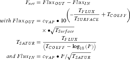 $$\eqalign{F_{net} &= Flux_{OUT} - Flux_{IN} \cr with\, Flux_{OUT} &= c_{VAP} \bullet 10^{\left(- \displaystyle{T_{FLUX} \over T_{SURFACE}} + T_{COEFF} \right)} \cr &\quad \times \bullet \sqrt{T_{Surface}} \cr T_{SATUR} &= \displaystyle{T_{FLUX} \over \left(T_{COEFF} - \log_{10} \left(P \right)\right)}\cr and\, Flux_{IN} &= c_{VAP} \bullet P /\sqrt{T_{SATUR}}}$$
The second method, within the acceptable range for δt, is to increase the number of particle initially loaded. In this way, the “representativeness” of the solutions found becomes more and more significant producing accurate results and can be found in other publications. The third way here examined is to verify how much an increase of the computational refinements mesh would add to the precision of the solutions. In these conditions, simulations have been run changing the radiation transport grid: 6 × 30, 12 × 30, and 18 × 30 cells have been tested producing the differences evident in Figure 12. So while the increase in computational mesh refines better the general shape of the crater (global error goes from 10−3 to 10−5%), in terms of maximum erosion differences are relatively small with respect to the much more coarse grid (i.e., 6 × 30), not really justifying its use, especially when compared to the computational time. The machine time in fact on Purdue CMUXE computational server assembled with Quad sockets AMD Opteron(TM) 6274 Interlagos 2.2 GHz having 16 cores for a total of 64 cores CPU total, has grown about nine times providing only a difference in the final erosion result of less than five percent. This results is well evident in Figure 13, allow for important considerations on the initial choices for the simulations.
(Color online) Calculated geometrical erosion evolutions along the plate in MK200-like conditions simulations using HEIGHTS-PIC (with δt = 10−6 μs and 6 × 30, 12 × 30, 18 × 30 grids).
(Color online) Calculated computational time in MK200-like conditions simulations using HEIGHTS-PIC on the CMUXE Server (Comparisons 6 × 30, 12 × 30, and 18 × 30).
In order to have more benchmarking comparisons, HEIGHTS-PIC has also been compared with the original HEIGHTS package for ELM conditions in Tokamaks (Sizyuk & Hassanein, Reference Sizyuk and Hassanein2010). Using ITER-like geometry, the evolution of an ELM event has been simulated for 100 µs. In particular, using the “ITER-FEAT Outline Design Report” (Aymar, 1001) as basic geometry for our simulations, carbon material divertor was assumed as target plate. The magnetic field intensity used is 5 T and the inclination of the field with respect to the target plate is 5°. The ELM impinging plasma has been simulated assuming an exponential beam shape with the maximum power density profile at the strike point. For the total duration, 12.6 MJ of energy (roughly 10% of the total pedestal energy) are supposed to reach the target plate (Harlow, Reference Harlow1963). The e-fold length of the power profile above the plate is in such conditions of 6.7 cm. At the strike point the power density profile peaks at 4.6 MW/cm2 with a minimum at the e-fold length of 1.692 MW/cm2. The ITER major radius is of 6.5 m while the assumed initial plasma temperature is of E 0 = 3.5 keV (Sizyuk & Hassanein, Reference Sizyuk and Hassanein2010; Aymar, Reference Aymar2001). The computational domain taken into account extends then for 6.7 cm along the target plate and for 15 cm perpendicular to it: 300 cells are used in the following ELM simulation making the cell dimensions of 0.67 cm for 0.5 cm. No poloidal magnetic field is assumed in HEIGHTS-PIC simulations.
Erosion of the divertor plate is highly influenced by the beam intensity, duration, and geometrical distribution above the target. Recent studies have pointed out that the plasma energy flux reaching the target plate through the scrape off layer has a non-symmetrical shape similar to an exponential decay.
The maximum erosion is then expected to be close to the strike point where the highest power flux is concentrated (Fig. 14). The time considered for a typical ELM event (100 µs) is too small to allow significant heat transfer through the material, so that most of the energy released is spent for the carbon erosion and its hydrodynamics movement in the plasma-vapor cloud above the surface. The profile at the end of the simulation performed with 95 sample particles (initial loading) and a grid of 10 cells along the target and 30 cells perpendicular to it, shows a maximum erosion value close to 0.06 µm close to the strike point as shown in Figure 13. As expected erosion is much less where the beam power deposition is less close to the end of examined plate length of 6.7 cm.
The maximum erosion value calculated by HEIGHTS-PIC is of the same order of magnitude to the one predicted by HEIGHTS (i.e., 0.18 µm (Sizyuk & Hassanein, Reference Sizyuk and Hassanein2010) but the footprint seems to be wider while the area covered by the profile itself seems to be a bit wider probably due to more energy reaching effectively the surface. During the impact duration of 0.1 ms, the impinging plasma initiates a strong surface vaporization. Most of the initial impact energy is spent in further eroding the carbon-based material close to the strike point. As vapor starts forming and becomes more dense the deceleration of the plasma particles interacting with the vapor, reduces the effective energy reaching the divertor (Fig. 15). The net erosion rate is then reduced with slight broadening effect toward the rest of the plate. As the vapor shields becomes more efficient in the screening effect, the broadening will become wider and wider since most of the energy directly impinging the plate mainly comes from the photons radiation and transport through less dense areas. Comparing in fact the integrated energy fluxes (Fig. 16), HEIGHTS-PIC shows a much higher radiation to the ground reaching the plate when compared to HEIGHTS (Sizyuk & Hassanein, Reference Sizyuk and Hassanein2010). At the same time the effective impacting integrated energy flux is of the same magnitude (at the peak 50 J/cm2 versus 80 J/cm2).
(Color online) HEIGHTS-PIC calculated divertor erosion in carbon plasma during an ELM in ITER-like conditions (GRID 10 × 30).
(Color online) HEIGHTS-PIC calculated erosion rate in carbon plasma during an ELM in ITER-like conditions (GRID 10 × 30).
(Color online) HEIGHTS-PIC calculated integrated energy fluxes in carbon plasma during an ELM in ITER-like conditions (GRID 10 × 30).
It is important to recall that in HEIGHTS-PIC simulations while the carbon vapor in front is well interpreted providing a close to target high dense and cool plasma (Hassanein & Konkashbaev, Reference Hassanein and Konkashbaev2003; Wurz et al., Reference Wurz, Pestchanyi, Landman, Bazylev and Kappler2001; Safronov et al., Reference Safronov, Arkhipov, Landman, Pestchanyi, Toporkov and Zhitlukhin2009; Pestchanyi et al., Reference Pestchanyi, Bazylev and Landman2004; Arkhipov et al., Reference Arkhipov, Bakhtin, Vasenin, Zhitlukhin, Kurkin, Safronov and Toporkov1999; Reference Arkhipov, Bakhtin, Vasenin, Zhitlukhin, Kurkin, Safronov and Toporkov2002), it is though unable to provide information about the plasma corona which considerably extends from the target (several cm), showing much higher temperatures and low densities and essentially formed by DT ions, electrons, and neutral particles. This is particularly evident when looking at the evolution of the carbon plasma vapor cloud close to the target. At the beginning (Fig. 17), as carbon plasma starts forming, it is mostly concentrated where the beam intensity is high (close to the striking point).
(Color online) HEIGHTS-PIC calculated density of the carbon plasma during an ELM in ITER-like conditions (GRID 10 × 30) at 1 µs.
As time progresses, other particles start being produced along the plate and the profile of the plasma density enlarges (Fig. 18): as time keeps progressing (Figs. 19 and 20), the carbon plasma vapor cloud tends to expand in both the X and Y directions. At the end of the simulation the carbon plasma/vapor front has reached about 3 cm from the plate while the cloud is relatively stationary over the divertor plate (Fig. 21). This distance is close to the evaluation provided for carbon vapor cloud (Hassanein & Konkashbaev, Reference Hassanein and Konkashbaev2003).
(Color online) HEIGHTS-PIC calculated density of the carbon plasma during an ELM in ITER-like conditions (GRID 10 × 30) at 25 µs.
(Color online) HEIGHTS-PIC calculated density of the carbon plasma during an ELM in ITER-like conditions (GRID 10 × 30) at 50 µs.
(Color online) HEIGHTS-PIC calculated density of the carbon plasma during an ELM in ITER-like conditions (GRID 10 × 30) at 75 µs.
(Color online) HEIGHTS-PIC calculated density of the carbon plasma during an ELM in ITER-like conditions (GRID 10 × 30) at 100 µs.
In the end, looking at the erosion profiles produced with longer ELMs (500 µs), we can see that similarities exist with the original HEIGHTS (Sizyuk & Hassanein, Reference Sizyuk and Hassanein2010). For longer ELM pulses (i.e., = 500 µs) the peak of the power flux close to the striking point reaches 0.92 MW/cm2. As expected, the maximum final erosion depth for the longer pulse is larger when compared to the shorter ELM (Fig. 22). Though for the areas of the target plate further from the striking point erosion is consistently less due to much less power flux effectively reaching the plate (Fig. 23). It is interesting to note also that the shift in position of the maximum depth is absent in HEIGHTS-PIC simulation because no poloidal field is present in the actual model and the diffusion across the magnetic field is not so pronounced to provoke erosion where the plate is not directly reached by the impinging beam. The trend compared with HEIGHTS is in good agreement in shape, magnitude and time evolution.
(Color online) HEIGHTS-PIC calculated erosion for different ELM pulses.
(Color online) HEIGHTS-PIC calculated erosion evolution for different ELM pulses.
5. CONCLUSIONS
ELMs and disruptions represent a serious problem for PFC during normal and abnormal operations in Tokamak devices. To evaluate the characteristics of this problem, a PIC method has been developed. The models in HEIGHTS-PIC provide through a novel use of the PIC technique a detailed picture of the plasma-vapor interaction and evolution during ELM events. Detailed plasma energy deposition model, thermal conduction, melting, evaporation and vapor expansion are included. The interaction of plasma with expanding vapor is examined for plasma energy transient deposition up to 0.1 ms. HEIGHTS-PIC was benchmarked against several other models in the well benchmarked Eulerian and Lagrangian original HEIGHTS package as well as experimental data provided by the plasma gun facility MK200 in Russia. It is shown a good agreement in the simulation of the plasma behavior during ELMs events and the overall divertor erosion profiles. Future work will extend the existing models improving the radiation transport part with the use of Monte-Carlo methods and parallelizing the structure of the code. The flexibility of PIC methods will be used in adapting complicated divertor/wall structures as well as nearby components to assess in detail the damage to these components as well. Additionally, more analysis for various ELMs and disruptions conditions will be analyzed and studied.
ACKNOWLEDGMENT
This work is supported by the US Department of Energy, Office of Fusion Energy Sciences.



