I. INTRODUCTION
Thin films are used in many modern high-tech systems.Reference Nix1–Reference Ramesh and Spaldin3 In these systems, distinct materials with specific differentiating properties are often mixed. Therefore, profound understanding of the mechanical behavior of these thin films is required to predict failure due to thermomechanical loading.Reference Nix1 Many materials behave differently than their bulk counterparts when one or more dimensions are in the range of an intrinsic length scale,Reference Thompson4–Reference Gruber, Böhm, Onuseit, Wanner, Spolenak and Arzt7 which is often the case for thin films. The mechanical behavior can also depend on the adjacent (adhered) films,Reference Arzt8 the film microstructure, and the fabrication process.Reference Freund and Suresh9 Therefore, experimental methods that can measure the mechanical performance of thin films in an accurate manner are of great value. The bulge test is such a valuable technique, acknowledged as one of the easier techniques to measure full (isothermal) stress–strain curves of freestanding thin films,Reference Vlassak and Nix10–Reference Xiang, Chen and Vlassak12 even partly into the compression regime.Reference Xiang and Vlassak13
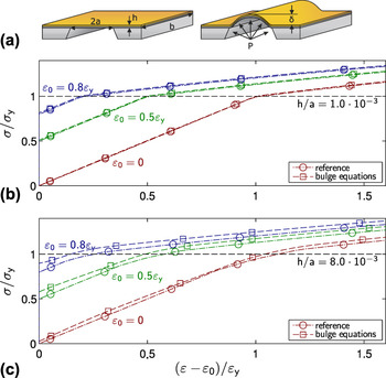
In the bulge test, a membrane is deflected using a pressurized medium, while the deflection is measured [Fig. 1(a)]. Typically, the stress and strain are calculated from the pressure P and out-of-plane deflection at the membrane apex δ by means of an analytical description of the membrane deformation, called the bulge equations.Reference Tsakalakos14, Reference Beams and Neugebauer15 These bulge equations are sensitive to the membrane geometry, which has been a source of inaccuracy for bulge test measurements in the past. However, with the currently available Si micromachining sample production techniques, these problems are largely overcome.Reference Vlassak and Nix10 Nevertheless, when material parameters obtained from bulge tests are compared with parameters obtained with other small-scale testing methods, such as nanoindentation, substrate warpage, or microbeam bending, some discrepancies emerge.Reference Small and Nix16, Reference Martins, Delobelle, Malhaire, Brida and Barbier17
(a) Schematic of a plane strain bulge test experiment. A slender rectangular membrane with width 2a and thickness h is deflected δ out-of-plane by a pressure P. (b, c) Stress–strain curves obtained by application of the bulge equations to a simulated virtual experiment (explained in the text), compared with the reference (input) stress and strain data, for a membrane thicknesses of 500 nm (b) and 5 μm (c).

Bulge test experiments can be classified with respect to the shape of the tested membrane (circular, rectangular, etc.). The plane strain bulge test, which uses a rectangular membrane with aspect ratio larger than 4,Reference Vinci and Vlassak5 is currently the most widely used bulge test for thin film testing, due to its favorable combination of microfabrication routes, its well-defined strain state (at least far away from the membrane boundaries), and its straightforward pressure versus deflection relationReference Vinci and Vlassak5, Reference Xiang, Chen and Vlassak12

where P is the pressure, a is the width of the membrane,  the Poisson’s ratio,
 is the initial residual (elastic) strain in the membrane, h the thickness of the film, δ the maximum deflection, and E Young’s modulus. Under the assumption that the membrane hinges freely at the boundaries (due to local plasticity and negligible bending stiffness of the thin film), the membrane profile is assumed to take the shape of the section of a cylinder. The stress σ and strain
 are then homogeneous through the major part of the membrane and are given by


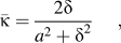
where  is the curvature of the (assumed) cylindrical shape of the loaded membrane. Note that any initially present strain (prestrain) in the membrane should be added to the bulge strain, i.e.,
 .
Figure 1 shows the results of a virtual bulge experiment, explained below, in which stress–strain curves obtained by applying the bulge equations [Eqs. (2)–(4)] to bulge profiles are compared to the reference (input) stress–strain behavior of the virtual experiment. Figure 1(b) confirms that the bulge equations adequately predict the stress and strain from the pressure and deflection for thin films of, e.g., 0.5 μm thickness, as reported in Xiang and Vlassak,Reference Xiang and Vlassak13 although a small (systematic) error can be noticed. Figure 1(c) shows, however, that this systematic error is significantly amplified when the bulge equations are applied on thicker films, e.g., of 5 μm thickness, which are for instance used in Micro-Electro-Mechanical Systems (MEMS) applications.Reference Bergers, Delhey, Hoefnages and Geers18 Note also that the systematic error increases when the membrane has some residual strain before starting the bulge test experiment. Residual strains are common in bulge membranes and are usually caused by the (large) thermal stresses during processing. Therefore, prestrains are often as high as 90% of the yield strain.Reference Xiang and Vlassak13 This triggers two important concerns: (i) it is unclear how the magnitude of these systematic errors depend on the membrane thickness and (ii) the error concentrates around the elastic regime, which is important for finding the elastic material parameters including the elastic limit and for which the larger measurement noise in bulge experiments can obscure such systematical errors.
The goal of this research was to identify and quantify these systematic errors to support the proper use and exploitation of the bulge test technique. At the same time, the regime where the (cylindrical) bulge equations are valid is identified.
Finite element method simulations are used to define a virtual experiment, allowing a comparison of the stress and strain taken directly from the simulation with the stress and strain calculated by the bulge equations (using the pressure-deflection data from the same simulation). This provides a direct comparison, eliminating all experimental uncertainties and enabling a detailed investigation of the systematic uncertainties in the bulge equations. Additionally, not only the deflection but also the shape of the profile of the loaded bulge membrane can be analyzed. The analysis will focus on the (“miniature”) plane strain bulge test because it is becoming increasingly more popular, yet the resulting conclusions apply to the bulge test in general. The “miniature” plane strain bulge test is described in Xiang et al.,Reference Xiang, Chen and Vlassak12 where the use of lithographic “micromachining” techniques allows for the fabrication of samples with very high dimensional accuracy, thereby greatly improving the accuracy of the method.
II. VIRTUAL EXPERIMENTS
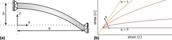
Due to symmetry, only half of the geometry of the miniature plane strain bulge test is modeled with eight-node quadratic quadrilateral elements. The symmetry edge is only confined in the x direction, whereas the other “clamped” edge is confined in the x and z directions while allowing contraction [Fig. 2(a)]. The validity of this “fully rigid” boundary condition was verified by performing two-dimensional (2D) simulations including the Si substrate. When the boundary is more compliant, the point of rotation (hinge) is moved further outward, creating a larger effective membrane width,  , which effects
 and
 through
 [Eqs. (2)–(4)]. However, the calculated effective bulge membrane width for simulations with the substrate was only 0.1% larger than for simulations with the fully rigid boundary conditions over the entire simulated
 range, which shows that the fully rigid boundary conditions are an adequate approximation. The dimensions of the modeled bulge membrane are taken equal to 6 mm by 1 mm. However, the membrane thickness to width ratio
 is varied to assess its effect on the validity regime of the bulge equations. The model was optimized for mesh convergence, resulting in a mesh of 600 by 2 elements in the x and z directions, respectively. Additional three-dimensional simulations were performed, including the Si substrate, which showed that the ratio between the principal strains in the center was
 for all ratios
 investigated in this work. Therefore, it is assumed that 2D plane strain simulations [Fig. 2(a)] are representative for the mechanical state at the center of these membranes.
(a) The simulated 2D model of half of the membrane, indicating the boundary conditions. (b) Stress–strain curves of the elastoplastic material model, illustrating the effect of the hardening parameter q.

Since the bulge test is often used to measure the elastoplastic response of thin films, the following typical elastoplastic material model was usedReference Xiang and Vlassak13



where  is the yield stress, E the Young’s modulus, and q a hardening exponent defining the hardening rate. Note that
 for
 , resulting in a purely elastic model and
 for
 , resulting in an ideal plastic model [Fig. 2(b)]. The base material parameters are chosen to simulate the material behavior of copper
 GPa,
 MPa,
 , and a Poisson’s ratio
 ,Reference Xiang and Vlassak13 although the influence of material parameters will be evaluated later over a wide range.
III. BULGE TEST ANALYSIS
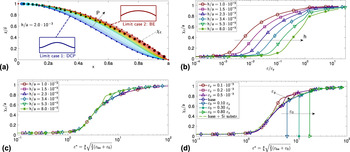
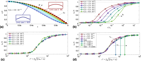
In Fig. 3(a), the bulge profiles for one specific thickness to width ratio  are plotted normalized with their maximum deflection δ. This figure shows the evaluation of the bulge profile shape for an increasing pressure P. It is obvious that not all profiles exhibit the cylindrical shape assumed by the bulge equations. Still, all profiles are bounded by a lower and upper limit case. Initially, at low pressures, there is no plasticity in the film, i.e., its deformation remains fully elastic, revealing the Double Clamped Plate (DCP) solutionReference Hetényi19 as the lower limit case. At a higher pressure, plasticity sets in at the clamped edge, initiating a plastic hinge, at which stage the profile shape starts to deviate from the DCP profile. Increasing the pressure further allows the plastic hinges to form completely, at which stage the profile deflects cylindrically; above that pressure, the assumptions in the bulge equations are valid. The two limit profiles, the DCP profile and the cylindrical shape of the bulge equations, can be expressed asReference Hetényi19


where M is the plane strain modulus, i.e.,  .
To quantify the transition from the DCP profile to the cylindrical profile, a cylindricity factor is introduced

where  is the smallest x-coordinate where the local curvature,
 , deviates more than 0.1% from the curvature in the center,
 .
The cylindricity can be interpreted as the relative part (around the bulge center) of the bulge profile that is cylindrical. Figure 3(b) shows the evolution of the cylindricity as a function of the (normalized) strain, for membranes with various thickness to width ratios  . All profiles start on the left side of the figure, where the cylindricity is close to zero. At a given strain, the cylindricity increases, which happens sooner for the thinner films, and a regime is entered where neither the DCP nor the bulge equations are accurate. Finally, when the global strain in the material is high enough, all membrane thicknesses reach the point where the cylindricity condition is fulfilled (i.e.,
 ).
Looking at the limit cases in more detail, the observation can be made that the DCP solution neglects the effect of membrane stress σm and only considers the effect of bending stresses σb, whereas the bulge equations do the opposite, neglecting σb and only considering σm. This argumentation suggests that the ratio of  could be a good candidate for the scaling of the cylindricity curves in Fig. 3(b). A scaling parameter can be extracted by analyzing the corresponding expressions of the (local) stresses
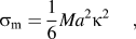
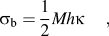
where σb is the bending stress at the (top) surface of the membrane under pure bending and  is the measured membrane curvature. Eq. (11) results from the Bulge Eqs. (2) and (3) under the assumption
 . The scaling ratio can then be expressed as
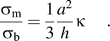
To allow experimentalists to calculate this ratio using their already available data, the above equation is written in terms of the strain that is obtained by the bulge equations. Therefore, an approximation of Eq. (3), i.e., 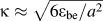 , is used to write:
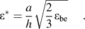
Figure 3(c) shows the same cylindricity curves as in Fig. 3(b), now plotted against the scaled strain  as defined in Eq. (14). It is seen that all profiles for different
 ratio fall on top of a scaled master curve. This is interesting, as Eq. (14) suggests that the scaling is nearly independent of the material parameters. To verify this, the elastoplastic material parameters are varied over a wide range. For all compared combinations of σy, M, and q, the scaled master plot is nearly identical [Fig. 3(d)]. For low
 , i.e., low σy and/or high M, plastic deformation initiates everywhere in the membrane before the plastic hinges at the boundaries are fully formed, resulting in a slight deviation from the master curve in the transition regime. Additionally, the figure shows the effect of prestrain (
 ) in the membrane, which causes the membrane to deform elastically until a threshold strain is reached, at which point the membrane profile “jumps” to the prestrain-free profile, after which it follows the master curve again.
(a) Evolution of the bulge profiles, for increasing pressure P, normalized with their deflection δ. The inset figures show the two limiting cases: (i) the DCP and (ii) the cylindrical shape of the Bulge Equations. The (color-coded) dots marked  are the limit positions, for which the curvature
 at the left side of the marker deviates less then 0.1% from the curvature in the center. (b) The “cylindricity” (i.e., the relative circular part) of each bulge profile as a function of the dimensionless strain
 for films with various thickness to width ratios
 . (c) The cylindricity
 of each bulge profile shifted to one master curve by plotting the curves of subfigure (b) as a function of the scaled strain. (d) The same master curve now for various material properties, where “base” refers to the reference copper material properties, “base + Si Substr.” refers to a simulation where the rigid boundary is replaced with the micromachined Si substrate. The variation of
 is achieved by both varying the Young’s modulus and the yield stress.

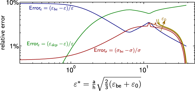
The scaled strain shifts all cylindricity curves to one master curve [Figs. 3(c) and 3(d)], which directly shows the validity regime of the bulge equations. In other words, the master curve allows the experimentalist to assess whether the assumptions in the bulge equations are valid for each bulge data point, measured at a certain strain, with a certain membrane geometry, and for certain material properties. Additionally, the errors as a result of using the bulge equations outside of this regime are quantified and plotted in Fig. 4. This logically shows that for small strains, the DCP solution is more accurate than the bulge equations, which start with a relative error in the strain of >9%. Nevertheless, the error in the stress  obtained with the bulge equations is relatively low from the start but increases around the curvature range where the bulge equations become valid. This error in the stress is slightly more pronounced if the prestrain in the membrane is larger. Exploiting the data beyond its validity regime yields an error, which is largest for the plane strain modulus, the initial membrane stress, and the yield strain. This is because, even for relatively unfavorable ratios of
 , at some point in the bulge test experiment, the plastic hinges start to form and with their evolution the corresponding error made by the bulge equations decreases. The result is that the systematic error is most severe in the low strain regime, where the modulus is usually fitted and which is used to backward extrapolate toward the unknown zero-stress state and the yield strain.Reference Xiang and Vlassak13
The relative systematic error in the stress  and strain
 obtained with the bulge equations and in the strain
 obtained with the DCP solution as a function of the scaled strain
 (compared with the reference stress and strain from the simulation). Additionally, the relative systematic error in the stress from the bulge equations is shown for various levels of prestrain (i.e.,
 ). Logically, for small strains, the DCP solution is more accurate in the strain than the bulge equations.

The relative systematic errors in strain and stress resulting from the bulge equations may not be acceptable. Since the systematic error under discussion in the article originates from the boundary conditions, a solution would be to measure the curvature and to calculate the stress directly from the curvature. To measure the strain in that same area of the membrane, a direct method like Digital Image Correlation can be used. This combination has been successfully applied on axisymmetrically inflated biomembranes at large strainsReference Hsu, Liu, Downs, Rigamonti and Humphrey20 and on micromachined SiN rectangular bulge membranes at small strains.Reference Neggers, Hoefnagels, Hild, Roux and Geers21
IV. CONCLUSIONS
Plane strain bulge test experiments are a valuable and acknowledged tool for measuring thin film properties. Yet, some quantitative mismatches exist in literature when comparing the results of the bulge tests with other small-scale tests, see, e.g., Small and NixReference Small and Nix16 and Martins et al.Reference Martins, Delobelle, Malhaire, Brida and Barbier17 One of the reasons for this is that the membrane deformation may be more complex than assumed, especially near the boundaries.
It was found that all bulge experiments start in a regime where the bulge equations are not valid, i.e., the DCP regime. When enough stress is applied to the system, plastic hinges start to form at the clamped edges initiating a transition regime. At some point, the plastic hinges have fully formed and the membrane profile deforms to a cylindrical profile, from which point onwards, the cylindricity assumption in the bulge equations is (sufficiently) valid.
A scaled strain is proposed that can be calculated from the measured deflection and the membrane thickness to width ratio. With this scaled strain, a master plot has been constructed that can be used to make a reliable assessment of the bulge test to identify the region where the data can be trusted. Finally, a solution is proposed to improve the accuracy of the bulge test method, especially for thicker films.