
1. Introduction
Turbulent flows exhibit nonlinear interactions over a wide range of spatiotemporal scales. In two-dimensional (2-D) decaying turbulence, the rate of energy dissipation is slowed considerably by kinetic energy transfer to large-scale coherent vortex cores through the inverse energy flux mechanism (Kraichnan Reference Kraichnan1967; McWilliams Reference McWilliams1990; Bracco et al. Reference Bracco, McWilliams, Murante, Provenzale and Weiss2000; Fox & Davidson Reference Fox and Davidson2010; Boffetta & Ecke Reference Boffetta and Ecke2012), while the enstrophy dissipation rate is enhanced by enstrophy transfer to small-scale eddies (Weiss Reference Weiss1991). The identification and modification of collective structures in the flow that accelerate or decelerate the inverse energy flux mechanism or alter the enstrophy cascade is a fundamental question (Hunt, Wray & Moin Reference Hunt, Wray and Moin1988; Holmes et al. Reference Holmes, Lumley, Berkooz and Rowley2012). This is unlikely to be addressed by flow-modification strategies based on linearization of the Navier–Stokes equations and reduced-order/surrogate representations that lack strict adherence to conservation laws. The objective of the current work is to tie a flow-modification strategy directly to the governing equations and their ensuing conservation laws.
A comparison of the behaviour of decaying 2-D turbulence with either well-developed vortices or phase-scrambled initial conditions revealed the crucial role of coherent vortex structures in suppressing the cascade rate (McWilliams Reference McWilliams1990). More recent studies by Jiménez (Reference Jiménez2020a,Reference Jiménezb) have shed light on the connections between dipoles (counter-rotating vortices) and streams (formed by the concatenation of dipoles) on the kinetic energy of the flow. These findings have been corroborated by network-theoretic approaches using induced velocity and flow perturbations (Yeh, Meena & Taira Reference Yeh, Meena and Taira2021). However, these recent data-intensive approaches require either machine learning to extract templates of dynamical significance or some explicit knowledge of vortical interactions in the flow. In the present work, we provide explicit physical definitions of forcing terms to be added to the Navier–Stokes equations, capable of altering conserved quantities independently, and revealing automatically the flow structures of significance.
Several previous efforts have focused on the exclusive modification of single conserved quantities in fluid flows. Vallis, Carnevale & Young (Reference Vallis, Carnevale and Young1989) and Shepherd (Reference Shepherd1990) modified the Euler equations to alter energy while preserving topological invariants associated with the vorticity field. This enabled the discovery of isolated energy extrema and stable steady equilibria. Sadourny & Basdevant (Reference Sadourny and Basdevant1985) designed, and Vallis & Hua (Reference Vallis and Hua1988) later employed, a subgrid-scale closure scheme that dissipates enstrophy while preserving energy. Another approach was developed by Gay-Balmaz & Holm (Reference Gay-Balmaz and Holm2013) and applied to dissipate the squared helicity while preserving energy in three-dimensional incompressible flow. A relevant early work with a more general context is that of Morrison (Reference Morrison1986). Our approach is inspired by the recently introduced framework of exterior dissipation (Aureli & Hanna Reference Aureli and Hanna2021; Hanna Reference Hanna2021), which enables proportional selective modification of multiple conserved quantities. We present local and global flow-modification approaches with three objectives: (i) to alter selectively and simultaneously any integral conserved quantities; (ii) to identify characteristic flow structures that accelerate or decelerate the inverse energy flux and enstrophy cascade; (iii) to discover and approach efficiently stable steady or slowly-varying states. In certain limits, our local approach leads to behaviour similar to that of Vallis et al. (Reference Vallis, Carnevale and Young1989) or Sadourny & Basdevant (Reference Sadourny and Basdevant1985).
2. Approach
We consider the 2-D flow of homogenous and incompressible fluid within a fixed bi-periodic square domain  $\mathcal {D}$. The governing dynamics is given by the forced Navier–Stokes equations
 \begin{equation} \frac{\partial \boldsymbol{u}}{\partial t} = \underbrace{- \boldsymbol{u} \boldsymbol{\cdot} \boldsymbol{\nabla} \boldsymbol{u} - \boldsymbol{\nabla} p / \rho }_{\boldsymbol{e}_{\boldsymbol{u}}} + \underbrace{\nu\,\nabla^2 \boldsymbol{u}}_{\boldsymbol{d}_{\boldsymbol{u}}} + \boldsymbol{f}_{\boldsymbol{u}},\quad \boldsymbol{\nabla} \boldsymbol{\cdot} \boldsymbol{u} = \boldsymbol{0}, \end{equation}
where  $\boldsymbol {u} = \boldsymbol {u} (\boldsymbol {x},t)$ is the velocity,
 $p$ is the pressure,
 $\rho$ is the density,
 $\nu$ is the kinematic viscosity, and
 $\boldsymbol {f}_{\boldsymbol {u}}$ is the external forcing to be designed. In the inviscid, unforced case, the flow admits the integral quadratic invariants
 $Q_i$ of kinetic energy
 $E$ and enstrophy
 $\varOmega$, defined as
 \begin{equation} Q_1 \equiv E = \int_{\mathcal{D}} \frac{1}{2}\,\boldsymbol{u} \boldsymbol{\cdot} \boldsymbol{u} \,\mathrm{d} \kern0.06em {\boldsymbol{x}}, \quad Q_2 \equiv \varOmega = \int_{\mathcal{D}} \frac{1}{2}\, \boldsymbol{\omega} \boldsymbol{\cdot} \boldsymbol{\omega} \,\mathrm{d} \kern0.06em {\boldsymbol{x}}, \end{equation}
where  $\boldsymbol {\omega } = \boldsymbol {\nabla } \times \boldsymbol {u} = \omega \hat {\boldsymbol {k}}$ is the vorticity field. We may express the time derivatives of these conserved quantities as
 \begin{equation} \frac{\mathrm{d}}{\mathrm{d}t}Q_i = \int_{\mathcal{D}} \boldsymbol{b}_i \boldsymbol{\cdot} \frac{\partial \boldsymbol{u}}{\partial t} \,\mathrm{d} \kern0.06em {\boldsymbol{x}} = \int_{\mathcal{D}} \boldsymbol{b}_i \boldsymbol{\cdot} \boldsymbol{e}_{\boldsymbol{u}} \,\mathrm{d} \kern0.06em {\boldsymbol{x}}+\int_{\mathcal{D}} \boldsymbol{b}_i \boldsymbol{\cdot} \boldsymbol{d}_{\boldsymbol{u}} \,\mathrm{d} \kern0.06em {\boldsymbol{x}} + \int_{\mathcal{D}} \boldsymbol{b}_i \boldsymbol{\cdot} \boldsymbol{f}_{\boldsymbol{u}} \,\mathrm{d} \kern0.06em {\boldsymbol{x}}. \end{equation}
The contribution of the Euler term in (2.3) vanishes (Hasegawa Reference Hasegawa1985; Foias et al. Reference Foias, Manley, Rosa and Temam2001), i.e.  $\int _{\mathcal {D}} \boldsymbol {b}_i \boldsymbol {\cdot } \boldsymbol {e}_{\boldsymbol {u}} \,\mathrm {d}\kern0.06em {\boldsymbol {x}} = 0$. The evolutions of kinetic energy and enstrophy are governed by
 $\boldsymbol {b}_{1} = \boldsymbol {u}$ and
 $\boldsymbol {b}_2 = \boldsymbol {\nabla } \times \boldsymbol {\omega }$, respectively; using a vector calculus identity,
 $\boldsymbol {\omega } \boldsymbol {\cdot } \boldsymbol {\omega } = \boldsymbol {\omega } \boldsymbol {\cdot } \boldsymbol {\nabla } \times \boldsymbol {u} = \boldsymbol {u} \boldsymbol {\cdot } ( \boldsymbol {\nabla } \times \boldsymbol {\omega } ) + \boldsymbol {\nabla } \boldsymbol {\cdot } (\boldsymbol {u} \times \boldsymbol {\omega })$, but due to the bi-periodic boundary conditions, the divergence term vanishes, and we have simply
 \begin{equation} \int_{\mathcal{D}}
\boldsymbol{\omega} \boldsymbol{\cdot} \boldsymbol{\omega}
\, \mathrm{d}\kern0.06em {\boldsymbol{x}} = \int_{\mathcal{D}}
\boldsymbol{u} \boldsymbol{\cdot} ( \boldsymbol{\nabla}
\times \boldsymbol{\omega} ) \,\mathrm{d}\kern0.06em
{\boldsymbol{x}}. \end{equation}
Along with (2.1), we also consider the forced vorticity transport equation in the form
 \begin{equation} \frac{\partial \omega}{\partial t} = \underbrace{ \frac{\partial \omega}{\partial y}\,\frac{\partial \psi}{\partial x} - \frac{\partial \omega}{\partial x}\,\frac{\partial \psi}{\partial y} }_{J(\omega,\psi)}+ \underbrace{ \nu\,\nabla^2 \omega }_{d_{\omega} } + f_\omega , \end{equation}
where 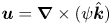 $\boldsymbol {u} = \boldsymbol {\nabla } \times (\psi \hat {\boldsymbol {k}})$ defines the streamfunction
 $\psi$, and
 $f_\omega$ is the external forcing to be designed. The integral kinetic energy and enstrophy invariants (Boffetta & Ecke Reference Boffetta and Ecke2012) and their time derivatives may be expressed as
 \begin{equation} Q_1 \equiv E = \int_{\mathcal{D}} \frac{1}{2}\,\omega \psi \,\mathrm{d} \kern0.06em {\boldsymbol{x}}, \quad Q_2 \equiv \varOmega = \int_{\mathcal{D}}\frac{1}{2}\,\omega^2 \,\mathrm{d} \kern0.06em {\boldsymbol{x}},\quad \frac{\mathrm{d}}{\mathrm{d}t}Q_i = \int_{\mathcal{D}} b_i\,\frac{\partial \omega}{\partial t} \,\mathrm{d} \kern0.06em {\boldsymbol{x}}, \end{equation}
where the energy has been rewritten by eliminating a divergence term due to the bi-periodic boundary conditions. Similarly to before,  $\int _{\mathcal {D}} b_i\,J(\omega, \psi ) \,\mathrm {d}\kern0.06em {\boldsymbol {x}} = 0$. Note that the
 $b_i$ in (2.6a–c) are distinct from the
 $\boldsymbol {b}_i$ in (2.3). We find that
 $b_1 = \psi$, by a manipulation of
 \begin{equation} \frac{\partial}{\partial t}\int_{\mathcal{D}} \left(\frac{1}{2}\,\boldsymbol{u} \boldsymbol{\cdot} \boldsymbol{u}\right)\, \mathrm{d} \kern0.06em {\boldsymbol{x}} = \int_{\mathcal{D}} \boldsymbol{\nabla} \times (\psi \hat{\boldsymbol{k}}) \boldsymbol{\cdot} \frac{\partial \boldsymbol{u}}{\partial t} \,\mathrm{d} \kern0.06em {\boldsymbol{x}} \end{equation}
and elimination of a divergence term, while clearly  $b_2 = \omega$.
The vector and scalar equations (2.1) and (2.5) will be the respective starting points for local and global approaches to systematically modify the inviscid conservation or viscous non-conservation of the integral quantities  $Q_i$. Each approach generates a unique forcing term, as described below.
2.1. Local formulation
We first construct an external forcing term  $\boldsymbol {f}_{\boldsymbol {u}}= \boldsymbol {f}_{\boldsymbol {u}}(\boldsymbol {x},t)$ in (2.1) using only local flow field information. Inspired by Hanna (Reference Hanna2021) and Aureli & Hanna (Reference Aureli and Hanna2021), we define
 \begin{equation} \boldsymbol{f}_{\boldsymbol{u}} ={-}\epsilon_1 (\boldsymbol{b}_1 \wedge \boldsymbol{b}_2) \boldsymbol{\cdot} \boldsymbol{b}_2 - \epsilon_2 (\boldsymbol{b}_2 \wedge \boldsymbol{b}_1) \boldsymbol{\cdot} \boldsymbol{b}_1, \end{equation}
where  $\boldsymbol {b}_1 = \boldsymbol {u}$ and
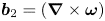 $\boldsymbol {b}_2 = ( \boldsymbol {\nabla } \times \boldsymbol {\omega } )$ as discussed above, and
 $\epsilon _1$ and
 $\epsilon _2$ are constant coefficients. The wedge product
 $\wedge$ of two vectors in three dimensions is
 $2\boldsymbol {b}_1 \wedge \boldsymbol {b}_2 = \boldsymbol {b}_1 \boldsymbol {b}_2 - \boldsymbol {b}_2 \boldsymbol {b}_1$, where juxtaposition indicates the standard tensor product. The terms in (2.8) can be rearranged into double cross-products:
 \begin{align} \boldsymbol{f}_{\boldsymbol{u}} ={-}\frac{\epsilon_1}{2}\underbrace{ \left( \| \boldsymbol{\nabla} \times \boldsymbol{\omega} \|^2\,\boldsymbol{u}- \left[ \boldsymbol{u} \boldsymbol{\cdot} \left( \boldsymbol{\nabla} \times \boldsymbol{\omega} \right)\right] \boldsymbol{\nabla} \times \boldsymbol{\omega} \right) }_{\boldsymbol{b}_2 \times (\boldsymbol{b}_1 \times \boldsymbol{b}_2 )} - \frac{\epsilon_2}{2} \underbrace{\left( \|\boldsymbol{u}\|^2\,\boldsymbol{\nabla} \times \boldsymbol{\omega} - \left[ \boldsymbol{u} \boldsymbol{\cdot} \left( \boldsymbol{\nabla} \times \boldsymbol{\omega} \right) \right] \boldsymbol{u} \right) }_{\boldsymbol{b}_1 \times (\boldsymbol{b}_2 \times \boldsymbol{b}_1)}. \end{align}
The first term exclusively alters the integral flow energy, while the second exclusively alters the integral flow enstrophy, allowing for independent manipulation of these two quantities. (The construction of  $\boldsymbol {b}_2$ involved the discarding of a divergence term. Thus the first term in
 $\boldsymbol {f}_{\boldsymbol {u}}$ does actually change the local vorticity magnitude and enstrophy, but its effect is a pure divergence that does not affect the global conservation.) If
 $\epsilon _1 = 0$, then energy is conserved, while enstrophy is increased (decreased) if
 $\epsilon _2 < 0$ (
 $\epsilon _2 > 0$). Similarly, if
 $\epsilon _2 = 0$, then enstrophy is conserved, while energy is increased (decreased) if
 $\epsilon _1 < 0$ (
 $\epsilon _1 > 0$). In what follows,
 $\epsilon _2 \ge 0$.
In the inviscid case, the rates of change of the integrals  $Q_i$ can be rearranged into the simple forms
 \begin{equation} \int_{\mathcal{D}} \boldsymbol{b}_i \boldsymbol{\cdot} \boldsymbol{f}_{\boldsymbol{u}} \,\mathrm{d} \kern0.06em {\boldsymbol{x}} ={-}\frac{\epsilon_i}{2} \int_{\mathcal{D}}\bigl[\boldsymbol{u} \times \left( \boldsymbol{\nabla} \times \boldsymbol{\omega} \right)\bigr]^2 \,\mathrm{d} \kern0.06em {\boldsymbol{x}} ={-}\frac{\epsilon_i}{2} \int_{\mathcal{D}} \left[\boldsymbol{u} \boldsymbol{\cdot} \boldsymbol{\nabla} \boldsymbol{\omega}\right]^2 \mathrm{d} \kern0.06em {\boldsymbol{x}}, \end{equation}
where we have used the fact that 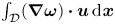 $\int _{\mathcal {D}} ( \boldsymbol {\nabla } \boldsymbol {\omega })\boldsymbol {\cdot } \boldsymbol {u} \,\mathrm {d}\kern0.06em {\boldsymbol {x}}$ vanishes for 2-D flow. These two rates are proportional, thus the quantity
 $E/\epsilon _1 - \varOmega /\epsilon _2$ is conserved (Hanna Reference Hanna2021), which seems to ensure that the resulting dynamics are not simply driven to a trivial equilibrium when both quantities are dissipated. The rates vanish when the two
 ${\boldsymbol {b}}_i$ align. Remarkably, when
 $\epsilon _2 = 0$, the rate of change of energy is the same as that generated by the method of Vallis et al. (Reference Vallis, Carnevale and Young1989), and when
 $\epsilon _1 = 0$, the rate of change of enstrophy is the same as that generated by the method of Sadourny & Basdevant (Reference Sadourny and Basdevant1985).
2.2. Global formulation
We next construct an alternative external forcing term 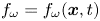 $f_{\omega } = f_{\omega }(\boldsymbol {x},t)$ in (2.5) incorporating global flow field information. Interpreting the integrals of (2.6a–c) as inner products of square-integrable functions on
 $\mathcal {D}$ allows for a formal analogy with the framework of Aureli & Hanna (Reference Aureli and Hanna2021), in which scalar fields are now regarded as infinite-dimensional vectors. We mimic the algebraic construction of exterior dissipation in Aureli & Hanna (Reference Aureli and Hanna2021) by introducing an array
 $\boldsymbol{\mathsf{B}} = (b_1, b_2) = (\psi, \omega )$ produced by stacking the vectors
 $b_i$, and the Gram matrix
 $\boldsymbol{\mathsf{G}}$ of the inner products of
 $b_1$ and
 $b_2$,
 \begin{equation} \boldsymbol{\mathsf{G}} = \int_{\mathcal{D}}\begin{bmatrix} \psi^2 & \psi \omega \\ \psi \omega & \omega^2 \end{bmatrix}\,\mathrm{d} \kern0.06em {\boldsymbol{x}}. \end{equation}
The global forcing is constructed as
 \begin{equation} f_\omega ={-}\tfrac{1}{2}\,\boldsymbol{\mathsf{B}} \,\mathrm{adj}(\boldsymbol{\mathsf{G}})\,\boldsymbol{\epsilon}, \end{equation}
where  $\mathrm {adj}(\cdot )$ denotes the adjugate (transpose of the cofactor matrix), and
 $\boldsymbol {\epsilon } = (\epsilon _1, \epsilon _2)$ is an array containing the constant coefficients exclusively modulating the rates of
 $E$ and
 $\varOmega$, respectively. Explicitly,
 \begin{equation} f_{\omega} ={-}\frac{\epsilon_1}{2}\left( \psi \int_{\mathcal{D}} \omega^2\,\mathrm{d} \kern0.06em {\boldsymbol{x}} - \omega \int_{\mathcal{D}} \psi \omega\,\mathrm{d} \kern0.06em {\boldsymbol{x}}\right) - \frac{\epsilon_2}{2}\left( \omega \int_{\mathcal{D}} \psi^2 \,\mathrm{d}\kern0.06em {\boldsymbol{x}} - \psi \int_{\mathcal{D}} \psi \omega\,\mathrm{d} \kern0.06em {\boldsymbol{x}} \right). \end{equation}
In the inviscid case, the rates of change of the integrals  $Q_i$ are
 \begin{equation} \int_{\mathcal{D}} b_i f_\omega \,\mathrm{d} \kern0.06em {\boldsymbol{x}} ={-}\frac{\epsilon_i}{2}\left(\int_{\mathcal{D}} \psi^2 \,\mathrm{d} \kern0.06em {\boldsymbol{x}} \int_{\mathcal{D}} \omega^2 \,\mathrm{d} \kern0.06em {\boldsymbol{x}}\right) \sin^2(\beta), \end{equation}
where  $\beta$ indicates the ‘angle’ between the vectors
 $b_i$ in the function space, defined by
 $\cos {\beta } = \int _\mathcal {D} \psi \omega \,\mathrm {d}\kern0.06em \boldsymbol {x} / \sqrt {\int _\mathcal {D} \psi ^2 \,\mathrm {d}\kern0.06em \boldsymbol {x} \int _\mathcal {D} \omega ^2 \,\mathrm {d}\kern0.06em \boldsymbol {x}}$. As before, the rates are proportional, vanishing when
 $\beta =0$ (when
 $\psi$ and
 $\omega$ ‘align’), and again the quantity
 $E/\epsilon _1 - \varOmega /\epsilon _2$ is conserved.
2.3. Viscous compensation
Both external forcing and viscosity break the invariance of conserved quantities. The forcing terms offer a means to compensate for viscous decay of energy and enstrophy, through the augmentation of the constant coefficients  $\epsilon _i$ by additional time-varying coefficients
 $\epsilon _i^\nu$ that can eliminate the effect of viscosity on these quantities or set their rates to some other desired behaviour. The rates of change of the conserved quantities with viscous compensation are
 \begin{equation} \frac{\mathrm{d}}{\mathrm{d}t}{Q}_i = D_i - \epsilon_i^{\nu} F\quad\Rightarrow\quad\epsilon_i^{\nu} = \frac{1}{F}\left( D_i - \frac{\mathrm{d}}{\mathrm{d}t}{Q}_i\right), \end{equation}
where  $D_i \equiv \int _{\mathcal {D}} \boldsymbol {b}_i \boldsymbol {\cdot } \boldsymbol {d}_{\boldsymbol {u}} \,\mathrm {d}\kern0.06em {\boldsymbol {x}}$ and
 $F \equiv - ({1}/{\epsilon _i})\int _{\mathcal {D}} \boldsymbol {b}_i \boldsymbol {\cdot } \boldsymbol {f}_{\boldsymbol {u}} \,\mathrm {d}\kern0.06em {\boldsymbol {x}}$ for the local formulation ((2.3) and (2.10)), while
 $D_i \equiv \int _{\mathcal {D}} b_i d_\omega \, \mathrm {d}\kern0.06em {\boldsymbol {x}}$ and
 $F \equiv -({1}/{\epsilon _i})\int _{\mathcal {D}} b_i f_\omega \,\mathrm {d}\kern0.06em {\boldsymbol {x}}$ for the global formulation ((2.6a–c) and (2.14)). Note that
 $F$ does not carry a subscript as it is the same for both quantities. As this shared forced rate
 $F$ tends to zero, compensation becomes impractical, requiring large coefficients
 $\epsilon _i^{\nu }$.
2.4. Numerical set-up
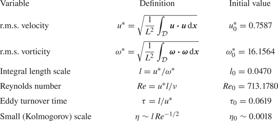
Two-dimensional direct numerical simulations are performed using a Fourier spectral method and a fourth-order Runge–Kutta time integration scheme on a square bi-periodic computational domain of sides  $L=1$ with
 $1024 \times 1024$ grid points in the
 $x$- and
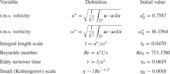
 $y$-directions. Further details of the set-up can be found in Taira, Nair & Brunton (Reference Taira, Nair and Brunton2016). The definitions of spatial and temporal scales, along with their initial values, are shown in table 1. The initial values are indicated with a subscript
 $0$. The spatial scales are normalized by the initial integral length scale
 $l_0$, and the time scales are normalized by the initial large-eddy turnover time
 $\tau _0$. The isotropic energy spectrum for 2-D turbulence is defined as
 $E(k) = {\rm \pi}k \langle |\hat {\boldsymbol {u}}(\boldsymbol {k})|^2 \rangle$ (where the average
 $\langle \cdot \rangle$ is over all
 $|\boldsymbol {k} | = k$) and
 $\hat {\boldsymbol {u}}(\boldsymbol {k}) = \int _{\mathcal {D}} \boldsymbol {u} (\boldsymbol {x})\,{\rm e}^{{\rm i} \boldsymbol {k} \boldsymbol {\cdot } \boldsymbol {x}} \,\mathrm {d}\kern0.06em {\boldsymbol {x}}$ (Boffetta & Ecke Reference Boffetta and Ecke2012). All the simulations are performed such that
 $k_{{max}} \eta \geq 8$, with
 $k_{{max}}$ the maximum resolvable wavenumber, and
 $\eta$ the smallest (Kolmogorov) length scale. The initial Reynolds number based on the integral length scale for all the viscous simulations is fixed at
 $Re_0 \approx 713.1780$.
Flow field parameters ( $L=1$).
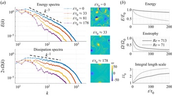
The initial condition for all the simulations is shown in figure 1(a). We also show corresponding energy spectra  $E(k)$, and dissipation (scaled enstrophy) spectra
 $2\nu \,\varOmega (k)$, with
 $\varOmega (k) = k^2\,E(k)$, as the unforced flow evolves. We can see the presence of the classical
 $k^{-3}$ turbulent energy spectra and
 $k^{-1}$ dissipation spectra at the initial condition of the turbulent flow, and the breakdown of the scaling leading to the eventual formation of large coherent structures. The evolution of energy
 $E$, enstrophy
 $\varOmega$, and integral length scale
 $l$ for two different Reynolds numbers over a long time period
 $0 \le t/\tau _0 \le 200$ is shown in figure 1(b). The rates of decay of energy (in particular) and enstrophy decrease with increasing
 $Re$.
Baseline (unforced) 2-D decaying homogeneous isotropic turbulent flow: (a) spectral evolution of energy and enstrophy, with plots of vorticity fields; (b) time history of energy, enstrophy and integral length scale for two different initial Reynolds numbers.

In the following section, we present and discuss the implications of local and global modification of inviscid, viscous, and compensated viscous flows. We define 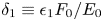 $\delta _1 \equiv \epsilon _1 F_0/E_0$ and
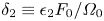 $\delta _2 \equiv \epsilon _2 F_0/\varOmega _0$ as normalized rates at which energy and enstrophy, respectively, are injected (negative) or extracted (positive). For the local formulation, the maximum resolvable wavenumber limits the maximum rates of modification.
3. Results and discussion
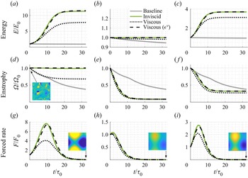
The effects of global forcing are shown in figure 2. The evolution of energy, enstrophy and the shared forced rate of change of these quantities  $F$ is shown over the time window
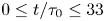 $0 \le t/\tau _0 \le 33$ for the unforced viscous baseline simulation (grey) and for the modified inviscid (green), viscous (black dotted) and compensated viscous (black dashed) flows. Three modification cases are shown: forced energy injection,
 $\delta _1 = -1$,
 $\delta _2 = 0$ (figures 2a,d,g); forced enstrophy dissipation,
 $\delta _1 = 0$,
 $\delta _2 = 1$ (figures 2b,e,h); and simultaneous forcing to inject energy and dissipate enstrophy,
 $\delta _1 = -1$,
 $\delta _2 = 0.25$ (figures 2c, f,i). Compensated viscous flows have an additional time-dependent modification to fully cancel the additional energy and enstrophy decay induced by viscous dissipation. The trajectories of these simulations are similar to those of the inviscid cases, although not identical, as the forcing is being applied to a different flow, albeit one with the same energy and enstrophy as the inviscid flow.
Trajectories of energy, enstrophy and the shared forced rate of change of these quantities for global forcing of 2-D turbulent flow: (a,d,g) modification of energy,  $\delta _1 = -1$,
 $\delta _2 = 0$; (b,e,h) modification of enstrophy,
 $\delta _1 = 0$,
 $\delta _2 = 1$; (c, f,i) modification of both quantities,
 $\delta _1 = -1$,
 $\delta _2 = 0.25$. The unforced viscous baseline simulation is shown in grey, the modified inviscid flow in green, viscous flows in black dotted, and compensated viscous flows in black dashed. Also shown in (g,h,i) (insets) are late-stage (
 $t/\tau _0 \approx 33$) vorticity snapshots for the globally modified viscous flows.
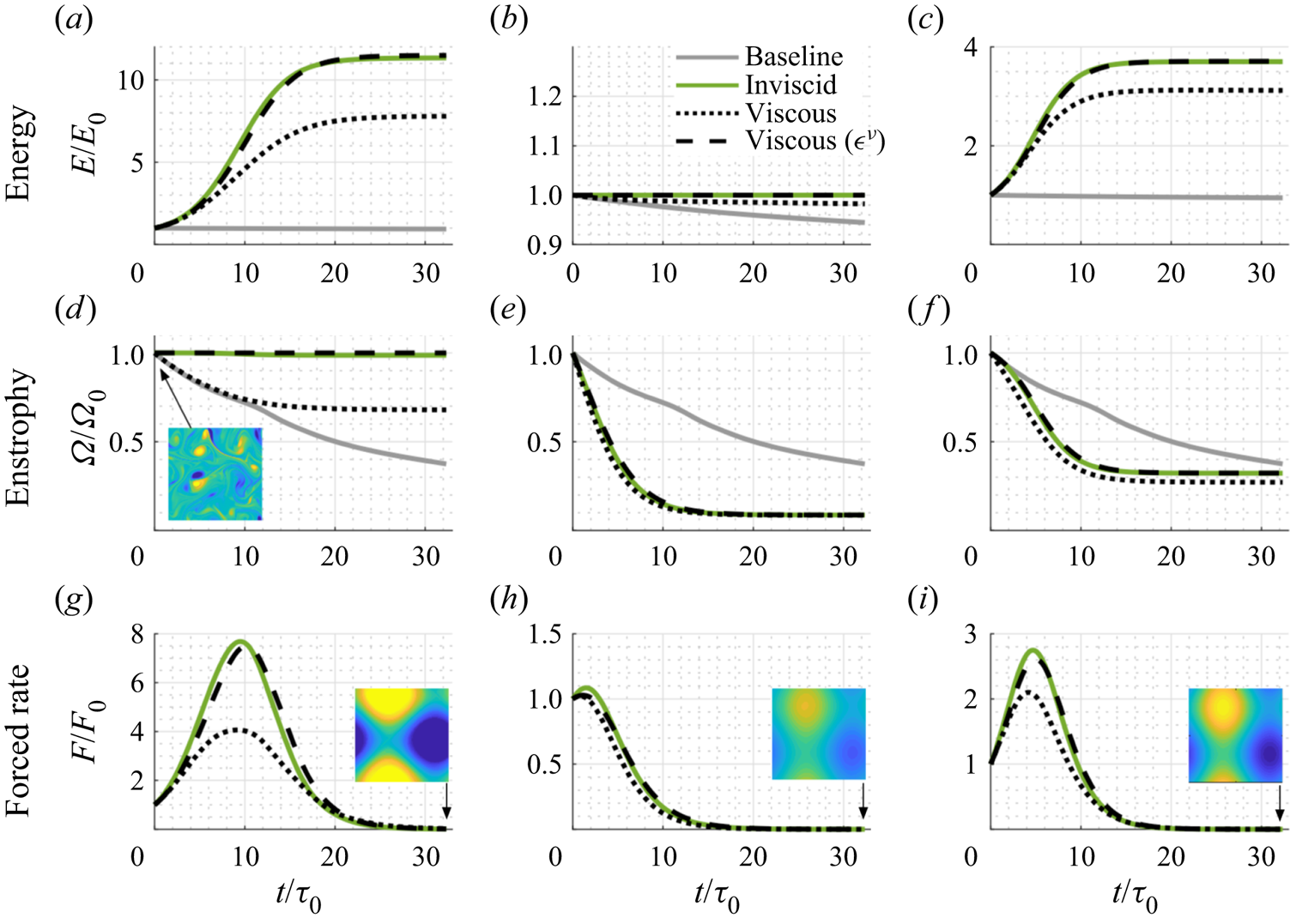
The maximum energy reached in figures 2(a,d,g) is higher for the inviscid flow than the viscous flow. The enstrophy is invariant in the inviscid setting, while for the viscous case, the enstrophy initially decays at the same rate as the baseline but quickly saturates to a nearly-constant value around  $t/\tau _0>10$. At this time, the forcing term
 $F$ reaches a peak and subsequently drops to zero as the system approaches a late-stage slowly decaying nearly steady state after
 $t/\tau _0>25$. Late-stage vorticity snapshots for the globally modified viscous flows are also shown. The inverse cascade in decaying turbulence leads to the formation of a dipole (Smith & Yakhot Reference Smith and Yakhot1993). The formation of this structure is accelerated with energy and enstrophy modification. The minimum enstrophy achieved in figures 2(b,e,h) is nearly identical for the inviscid and viscous flows, with a nearly-steady state reached quickly around
 $t/\tau _0>10$. The mixed case in figures 2(c, f,i) shares a combination of the features observed in figures 2(a,d,g) and 2(b,e,h).
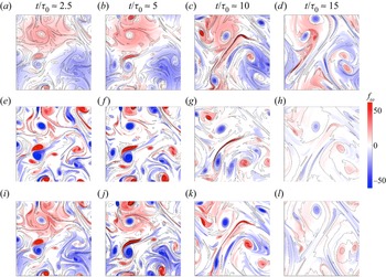
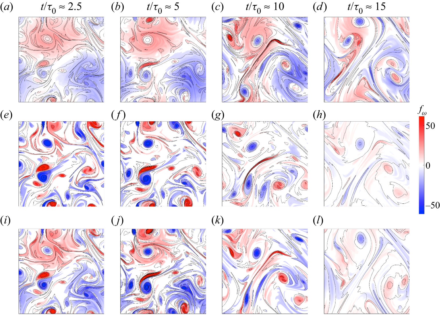
Shown in figure 3 is the global forcing  $f_\omega$ at several times, superimposed on vorticity contours. We observe that energy modification excites streams (fast regions between vortex dipoles) and some other more diffuse regions between vortex cores, while enstrophy modification excites vortex cores. This is consistent with the conclusions from Jiménez (Reference Jiménez2020a) and McWilliams (Reference McWilliams1990), where streams and vortex cores were found to be the relevant structures correlated with energy and enstrophy, respectively. As the solution approaches the late-stage flow, the forcing inputs fade, and indeed vanish in the inviscid case. All of the forced cases approach a non-trivial steady or slowly-varying state with a characteristic length scale of the order of the system size.
Forcing fields  $f_\omega$ superimposed on vorticity contours (black) for global forcing of 2-D turbulent flow: (a–d) modification of energy,
 $\delta _1 = -1$,
 $\delta _2 = 0$; (e–h) modification of enstrophy,
 $\delta _1 = 0$,
 $\delta _2 = 1$; (i–l) modification of both quantities,
 $\delta _1 = -1$,
 $\delta _2 = 0.25$.
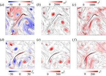
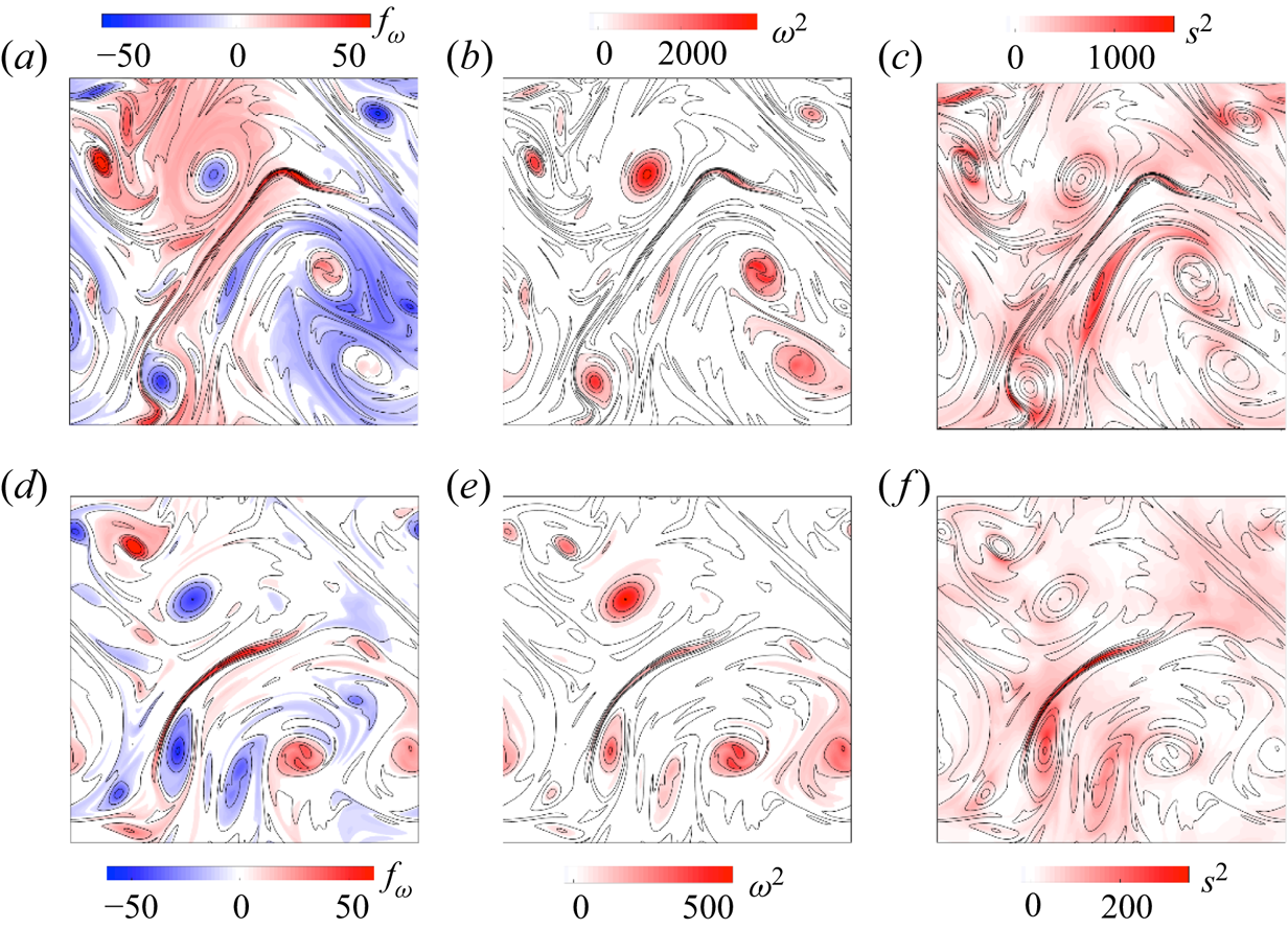
For the energy modification and enstrophy modification cases, we compare the global forcing  $f_\omega$ with the enstrophy field and a scalar measure of the strain field in figures 4(a–c) and 4(d–f), respectively, at
 $t/\tau _0 \approx 10$. The enstrophy field
 $\boldsymbol {\omega }^2$ can be computed easily from the vorticity. For 2-D incompressible flow, an appropriate invariant measure of strain (Weiss Reference Weiss1991; Oetzel & Vallis Reference Oetzel and Vallis1997) is the determinant of (twice) the symmetric part of the velocity gradient tensor
 $\boldsymbol{\varSigma}$, given by
 \begin{align} \boldsymbol{\varSigma} =
\begin{bmatrix} \dfrac{\partial u}{\partial x} &
\dfrac{\partial u}{\partial y} \\ \dfrac{\partial
v}{\partial x} & \dfrac{\partial v}{\partial y}
\end{bmatrix}.
\end{align}
We employ  $s^2 \equiv - \mathrm {det} (\boldsymbol{\varSigma} + \boldsymbol{\varSigma}^{\rm T} )$. The energy forcing operates both in regions of significant strain and vorticity, while the enstrophy forcing is, not surprisingly, more strongly associated with the latter. It is clear that the forcing fields are distinct from either of the two measures.
(a,d) The forcing field  $f_\omega$, (b,e) the enstrophy field
 $\boldsymbol {\omega }^2$, and (c, f) the strain field
 $s^2$, superimposed on vorticity contours (black) at
 $t/\tau _0 \approx 10$ for (a–c) modification of energy,
 $\delta _1 = -1$,
 $\delta _2 = 0$, and (d–f) modification of enstrophy,
 $\delta _1 = 0$,
 $\delta _2 = 1$.
To quantify the influence of the rate parameters  $\delta _1$ and
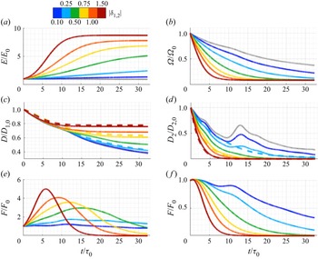
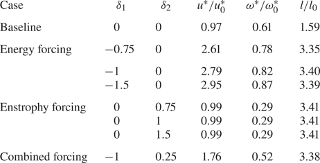
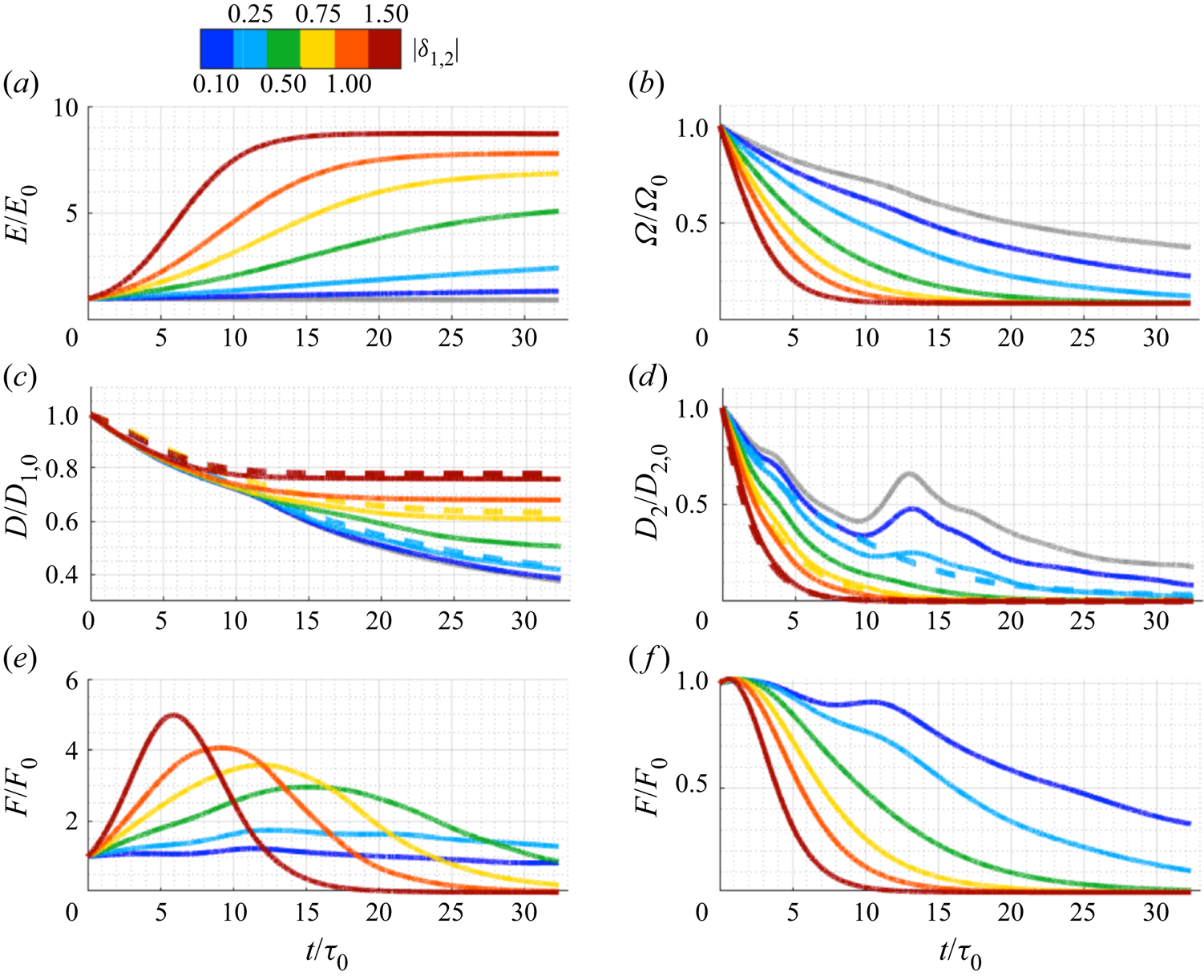
 $\delta _2$ on the system trajectories, we run additional simulations for energy and enstrophy modification as shown in figures 5(a,c,e) and 5(b,d, f), respectively. For energy modification, we can see that late-stage energy saturates at different values for different forcing
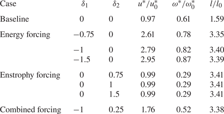
 $\delta _1$. However, for enstrophy modification, the enstrophy trajectories saturate to the same level. This is also evident in the values of velocity and vorticity magnitude of late-stage flow fields at
 $t/\tau _0 = 30$ in table 2. The integral length scale at this late stage is nearly identical for all modified cases. As seen in table 2, the mixed case leads to lower values of vorticity and velocity than the purely energy-modified case.
Influence of rate parameters ( $\delta _1$ and
 $\delta _2$) on global forcing of 2-D turbulent flow: (a,c,e) modification of energy, and (b,d, f) modification of enstrophy. Trajectories of energy/enstrophy, viscous decay rate, and the forced rates of change of these quantities are shown. The unforced viscous baseline simulation is in grey. The dashed lines in (c,d) are empirical fits to scaling laws, discussed in the text.
Values at  $t/\tau _0 \approx 30$.
We also show the viscous decay rate  $D_i = \int _{\mathcal {D}} b_i d_\omega \,\mathrm {d}\kern0.06em {\boldsymbol {x}}$ for energy and enstrophy modification in figures 5(c,d). We see that for the baseline flow, the viscous energy decay rate decreases monotonically, while the viscous enstrophy rate initially decreases, then increases to a peak value around
 $t/\tau _0 = 26$, and subsequently decreases again. For cases with
 $\delta _2 \ge 0.5$, the non-monotonic behaviour in the decay rate disappears. The viscous enstrophy decay rate for the baseline flow follows
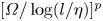 $[\varOmega /\log (l/\eta )]^p$, where
 $p = 3/2$ (Davidson Reference Davidson2015). For the modified flows, we find empirically
 $p = 1.66$, 2.42 and
 $3.00$ for
 $\delta _2 = 0.25$, 0.5 and
 $0.75$, respectively. As shown by the dashed lines, the viscous energy decay rate for modified flows follows
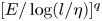 $[E/\log (l/\eta )]^q$, where
 $q = -1.0$,
 $-0.24$ and
 $-0.12$ for
 $\delta _1 = 0.5$, 0.75 and
 $1.5$, respectively. The forced rates for various cases are shown in figures 5(e, f). For the cases with
 $\delta _1 \le 0.25$, viscous dissipation effects dominate the external energy forcing input, and correspondingly the flow does not show large changes in energy. For
 $\delta _1 \ge 0.5$, a peak in the shared forced rate is observed. The times corresponding to the peaks decrease with increasing
 $\delta _1$, reflecting a more rapid approach to late-stage behaviour.
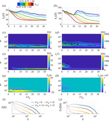
In decaying turbulence, energy accumulates in the smallest wavenumber  $k_{min} \approx 1/L$, leading to condensate formation (Boffetta & Ecke Reference Boffetta and Ecke2012). The formation of the condensate is accelerated with the modification of energy and enstrophy. We show the centroid wavenumbers of the energy spectra
 $k_c (E)$ and enstrophy spectra
 $k_c (\varOmega )$ for the energy and enstrophy modified cases in figures 6(a) and 6(b), respectively. Here,
 $k_c(E) = \int _{0}^{k_{max}}k\,E(k)\,{\rm d}k / \int _{0}^{k_{max}}E(k)\,{\rm d}k$ and
 $k_c(\varOmega ) = \int _{0}^{k_{max}}k\,\varOmega (k)\,{\rm d}k / \int _{0}^{k_{max}}\varOmega (k)\,{\rm d}k$. As the flow evolves, the baseline flow centroid energy and enstrophy wavenumbers both decrease non-monotonically (McWilliams Reference McWilliams1990). This non-monotonicity is suppressed for modified flows with
 $\delta _2 \ge 0.5$.
Influence of rate parameters ( $\delta _1$ and
 $\delta _2$) on spectra for global forcing of 2-D turbulent flow. Centroid wavenumbers of (a) energy and (b) enstrophy spectra, with the unforced viscous baseline in grey. Baseline flow spectrograms of (c) energy and (d) enstrophy. Spectrograms of (e) energy and (g) energy transfer in the energy-modified case
 $\delta _1=-1$, and ( f) enstrophy and (h) enstrophy transfer in the enstrophy-modified case
 $\delta _2=1$. Spectral evolution for (i) the energy-modified case
 $\delta _1=-1$, and (j) the enstrophy-modified case
 $\delta _2=1$.
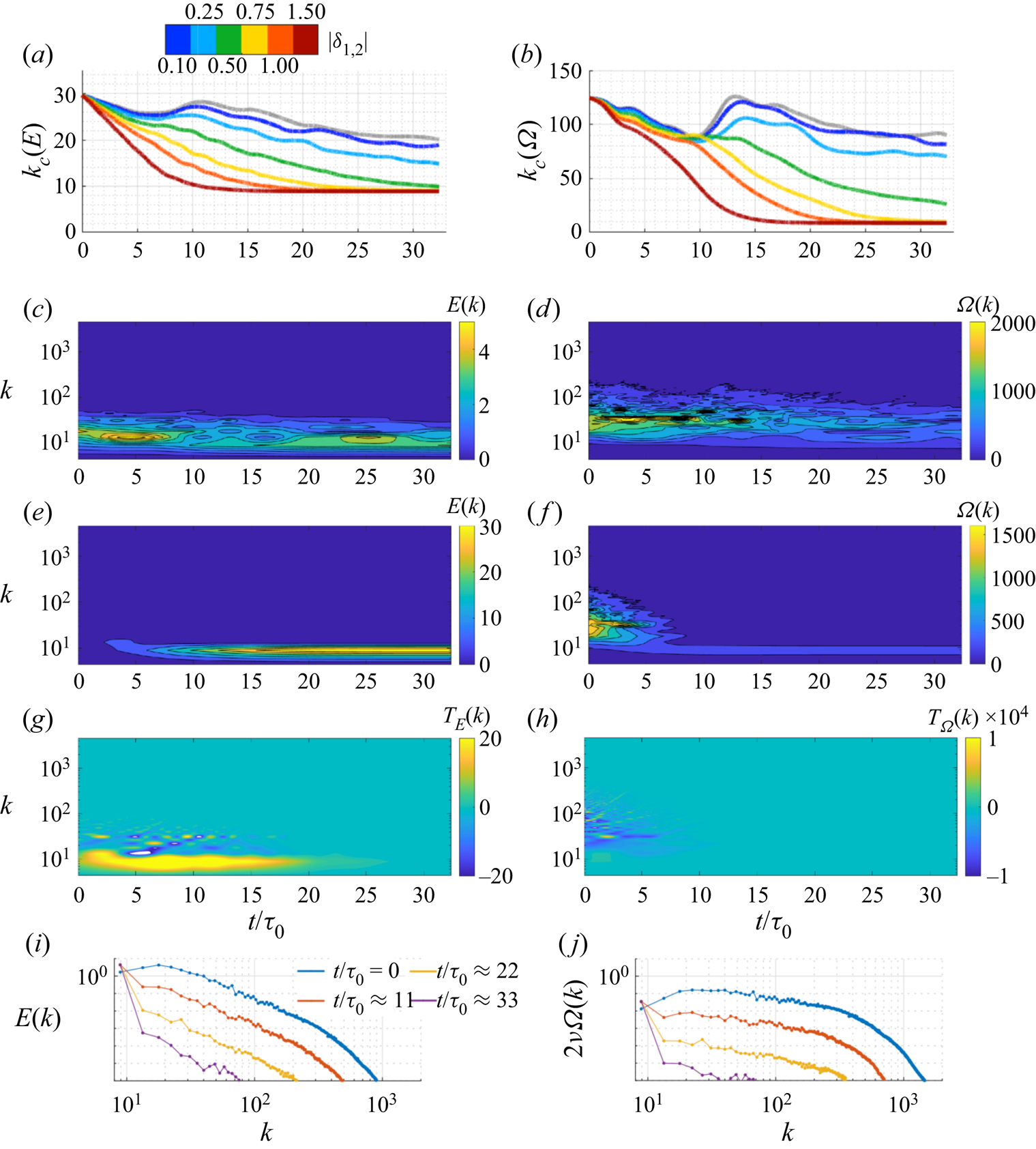
We show the spectrogram of energy and enstrophy for baseline flow in figures 6(c) and 6(d), respectively, and for the modified energy with  $\delta _1 = -1$ in figure 6(e) and modified enstrophy with
 $\delta _2=1$ in figure 6( f). (Slices through figures 6(e, f) can be seen in figures 6(i,j).) We can see here the distribution of energy in the range of wavenumbers
 $k \approx 10\unicode{x2013}50$ and the distribution of enstrophy in the range
 $k \approx 50\unicode{x2013}150$. Both the centroid plots and spectrograms show rapid shifts towards low wavenumbers for the modified energy and enstrophy. We also show the transfer of energy
 $T_E(k,t) = {\partial E(k)}/{\partial t} + 2 \nu k^2\,E(k)$ and enstrophy
 $T_\varOmega (k,t) = {\partial \varOmega (k)}/{\partial t} + 2 \nu k^2\,\varOmega (k)$ in figures 6(g) and 6(h) for the respective modified cases. There is a large positive transfer of energy to smaller wavenumbers for energy modification throughout the entire time period considered, while for enstrophy modification, the transfers die out fairly quickly.
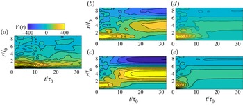
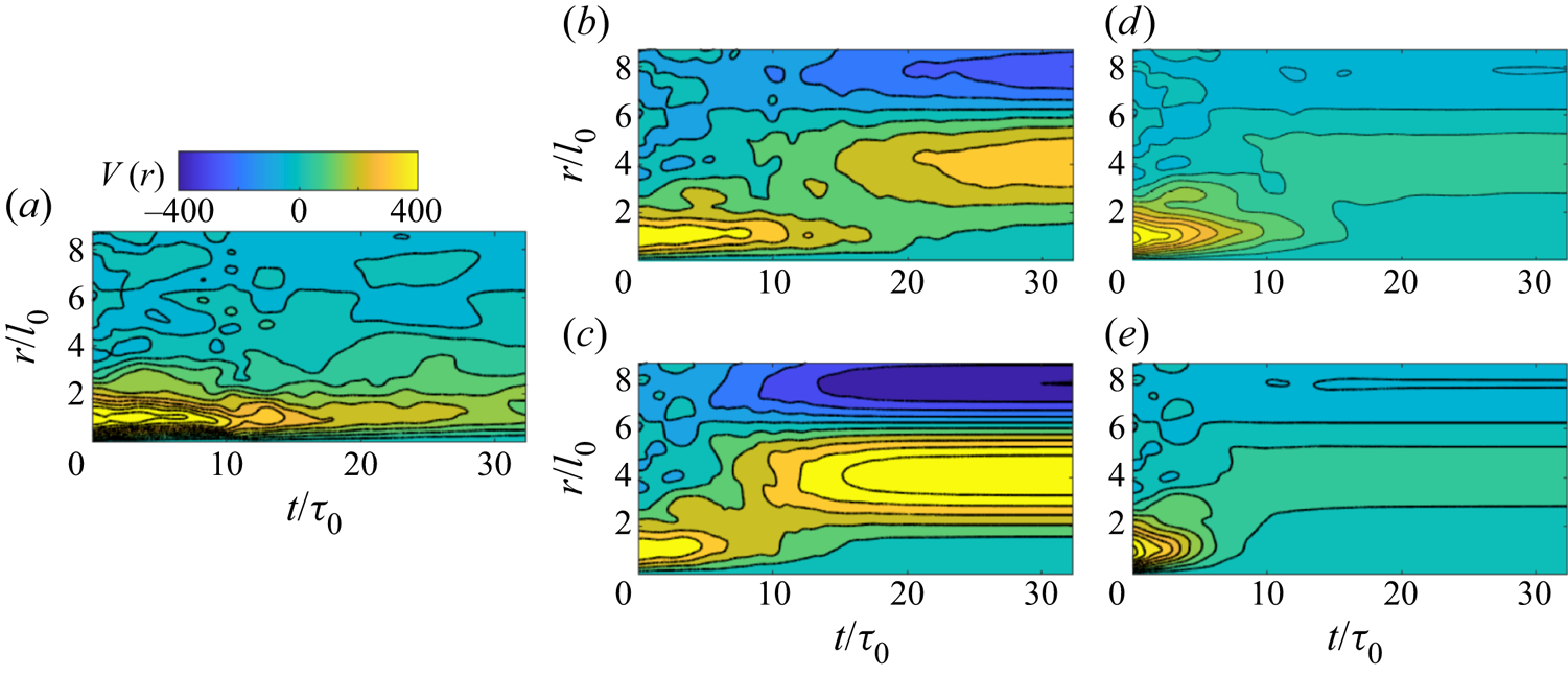
To illustrate further these effects of the modification in the physical domain, we compute the 2-D signature function  $V(r) = \int _0^{k_{max}} E(k)\,{\rm J}_3(kr)\,k \,\mathrm {d}k$, where
 ${\rm J}_3$ is a Bessel function of the first kind. This function represents the measure of energy held in eddies of size
 $r$, and is related to the second-order structure function of the flow (Davidson Reference Davidson2015). The signature function for the baseline flow is shown in figure 7(a). The energy modification cases with
 $\delta _1 = -0.5$ and
 $-1$ are shown in figures 7(b) and 7(c), respectively. The enstrophy modification cases with
 $\delta _2 = 0.5$ and
 $\delta _2 = 1$ are shown in figures 7(d) and 7(e), respectively. Initially, much of the energy in the baseline flow is concentrated near the initial integral length scale
 $r \approx l_0$. As the modified flows evolve, energy gets distributed across eddies of different sizes, with a shift towards larger sizes. As the energy of the flow increases for energy-modified cases, we see a larger magnitude associated with the signature function. The energy is unaffected by forcing in the enstrophy modification cases, so the corresponding energy level decreases, as in the baseline flow.
Two-dimensional signature function  $V(r)$ (see text) for (a) baseline, energy modification with (b)
 $\delta _1=-0.5$ and (c)
 $\delta _1 = -1$, and enstrophy modification with (d)
 $\delta _2 = 0.5$ and (e)
 $\delta _2 = 1$.
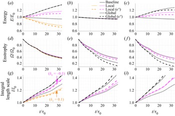
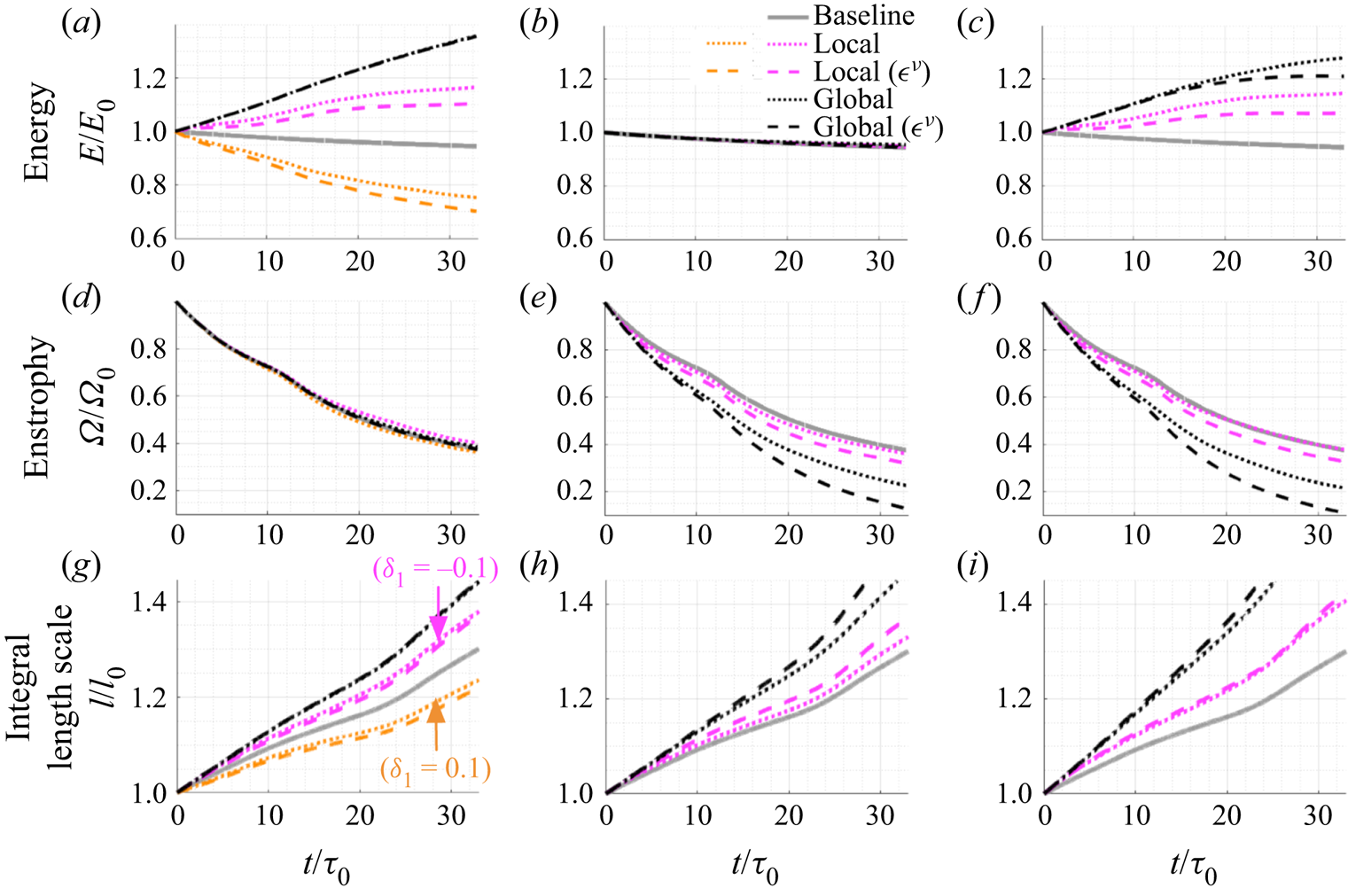
The effects of local forcing are shown in figures 8 and 9, and compared with the global forcing in figure 8. The evolution of energy, enstrophy and the integral length scale is shown over the time window 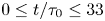 $0 \le t/\tau _0 \le 33$ for the unforced viscous baseline simulation (grey) and for the locally (magenta or orange) and globally (black) modified viscous (dotted) and compensated viscous (dashed) flows. Three modification cases are shown: forced energy injection
 $\delta _1 = -0.1$,
 $\delta _2 = 0$, magenta, or dissipation
 $\delta _1 = 0.1$,
 $\delta _2 = 0$, orange (figures 8a,d,g), forced enstrophy dissipation
 $\delta _1 = 0$,
 $\delta _2 = 0.1$ (figures 8b,e,h), and simultaneous forcing to inject energy and dissipate enstrophy
 $\delta _1 = 0.1$,
 $\delta _2 = 0.25$ (figures 8c,f,i). Here, the compensated viscous flows are designed so that the viscous contribution to the decay of energy and enstrophy matches that of the unforced baseline flow. The forcing coefficients are smaller than those used in figure 2 because the achievable rate of local forcing is limited by the maximum resolvable wavenumber. Therefore, the systems do not approach late-stage behaviour in this time window.
Comparison of local and global forcing of 2-D turbulent flow: (a,d,g) modification of energy,  $\delta _1 = -0.1$,
 $\delta _2 = 0$ (magenta),
 $\delta _1 = 0.1$,
 $\delta _2 = 0$ (orange); (b,e,h) modification of enstrophy,
 $\delta _1 = 0$,
 $\delta _2 = 0.1$; (c, f,i) modification of both quantities,
 $\delta _1 = -0.1$,
 $\delta _2 = 0.1$. Trajectories of energy, enstrophy and the integral length scale are shown for the unforced viscous baseline simulation (grey) and for the the locally (magenta or orange) and globally (black) modified viscous (dotted) and compensated viscous (dashed) flows.
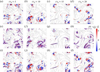
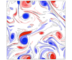
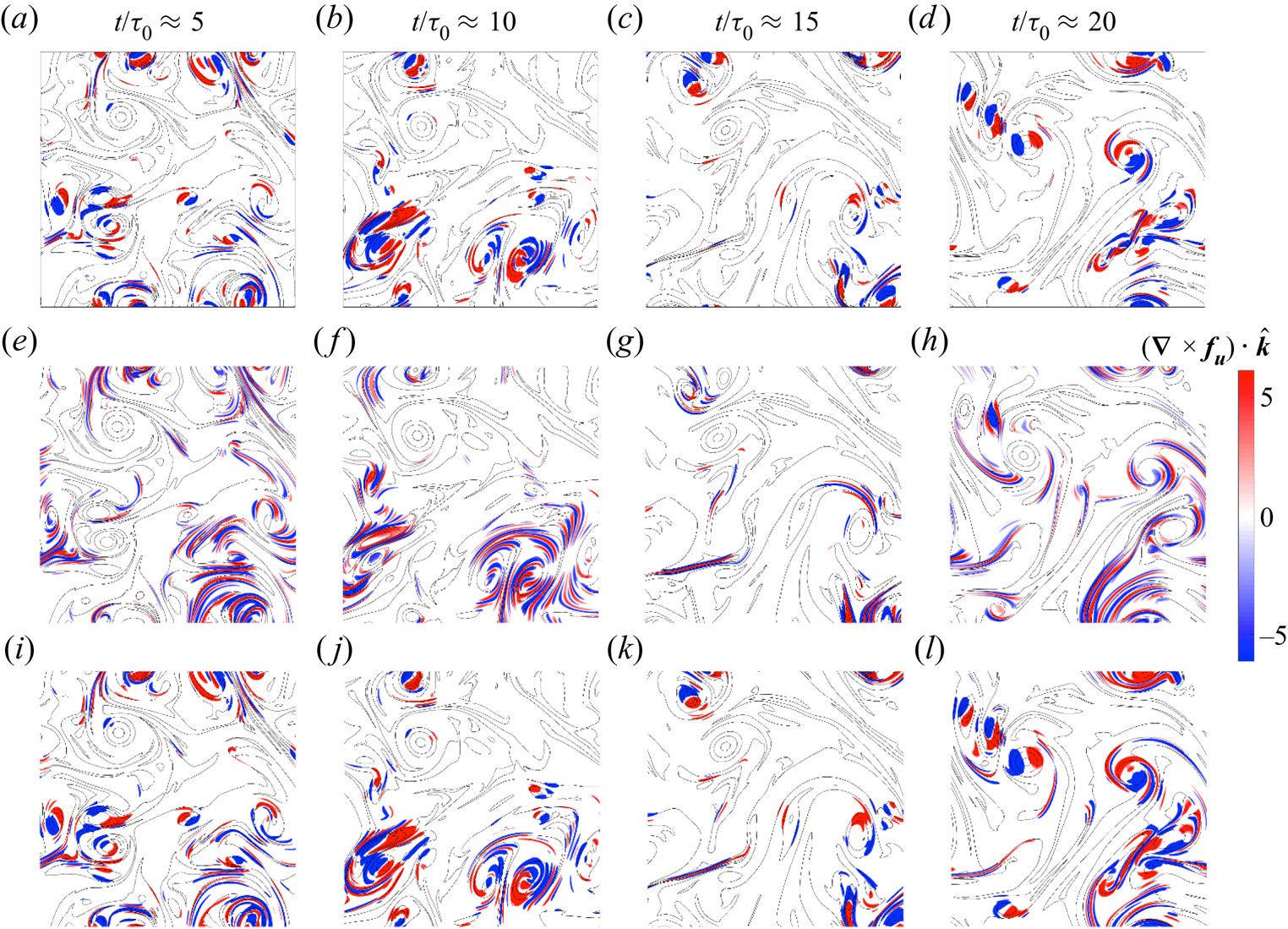
Forcing fields  $(\boldsymbol {\nabla } \times \boldsymbol {f}_{\boldsymbol {u}}) \boldsymbol {\cdot } \hat {\boldsymbol {k}}$ superimposed on vorticity contours (black) for local forcing of 2-D turbulent flow: (a–d) modification of energy,
 $\delta _1 = -0.1$,
 $\delta _2 = 0$; (e–h) modification of enstrophy,
 $\delta _1 = 0$,
 $\delta _2 = 0.1$; (i–l) modification of both quantities,
 $\delta _1 = -0.1$,
 $\delta _2 = 0.1$.
We find that the global forcing is significantly more effective than the local forcing in changing the quantities of interest. In particular, the effect of the local modification on enstrophy in figures 8(e) and 8(f) is weak. The behaviour of the integral length scales is curious. Note that the integral length scale is simply the square root of the ratio of energy to enstrophy. As shown earlier, in figure 1, lower Reynolds number baseline flows are characterized by faster decay of both energy and enstrophy, and more rapid growth of integral length scale. Yet figures 8(a,d,g) show that when we decrease (orange) or increase (magenta) the energy through forcing, this decelerates or accelerates, respectively, the growth of the integral length scale.
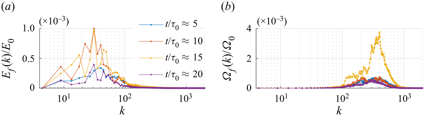
Figure 9 shows the local forcing  $(\boldsymbol {\nabla } \times \boldsymbol {f}_{\boldsymbol {u}}) \boldsymbol {\cdot } \hat {\boldsymbol {k}}$ at several times for the locally modified viscous flows with energy injection and/or enstrophy dissipation. These local forcing fields are significantly different from the global ones in figure 3. Energy modification introduces new dipolar structures near existing vortex cores, while enstrophy modification introduces streaky elongated dipolar structures between the cores. These streaks help the filamentation process of vorticity, accelerating the enstrophy cascade (Davidson Reference Davidson2015). The latter is reminiscent of recent findings using broadcast mode analysis (Yeh et al. Reference Yeh, Meena and Taira2021), where streaks occupying low-vorticity regions were found to be the most sensitive structures to flow perturbations. The forcings have spectra
 $E_f(k) = {\rm \pi}k \langle |\hat {\boldsymbol {f}_{\boldsymbol {u}}}(\boldsymbol {k})|^2 \rangle$ (where the average
 $\langle \cdot \rangle$ is over all
 $|\boldsymbol {k} | = k$) and
 $\varOmega _f(k) = k^2\,E_f(k)$, shown in figure 10 for the two pure cases. They evolve non-monotonically. These modifications are characterized by wavenumbers
 $k$ below
 ${\approx }100$ and above
 ${\approx }100$ for enstrophy. This difference reflects the simultaneous acceleration of the inverse energy and enstrophy fluxes to larger and smaller scales, respectively.
Spectra (arbitrary units) corresponding only to the forcing-induced velocity in locally modified viscous flows at several times: (a) forced energy spectrum from modification of energy,  $\delta _1 = -0.1$,
 $\delta _2 = 0$; (b) forced enstrophy spectrum from modification of enstrophy,
 $\delta _1 = 0$,
 $\delta _2 = 0.1$.

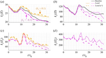
Figure 11 shows the influence of local energy and enstrophy modification on the spectral statistics of the flow. In particular, we show the centroid energy and enstrophy wavenumbers in figures 11(a,b), similar to figures 6(a,b). We also show the centroid wavenumbers of the forcing fields for energy- and enstrophy-modified cases. We see that for  $\delta _1 = -0.1$, the energy transfers to smaller wavenumbers compared to the baseline, resulting in acceleration of the inverse energy flux, while for
 $\delta = 0.1$, energy transfers to higher wavenumbers compared to the baseline, slowing down the inverse flux cascade. For the enstrophy modification, we see that although initially the centroid wavenumbers are identical, the enstrophy transfers to lower wavenumbers than the baseline. The corresponding centroid of the wavenumbers of energy forcing lies in the range
 $50 \le k_c(E_f) \le 120$ (corresponding to the elongated dipoles), while the centroid of the wavenumbers of enstrophy forcing lies in the range
 $200 \le k_c(E_f) \le 400$, corresponding to the elongated streaks.
Centroid wavenumbers for: (a,c) modification of energy,  $\delta _1 = -0.1$,
 $\delta _2 = 0$ (magenta),
 $\delta _1 = 0.1$,
 $\delta _2 = 0$ (orange); (b,d) modification of enstrophy,
 $\delta _1 = 0$,
 $\delta _2 = 0.1$. (a,b) Centroid energy and enstrophy centroid wavenumbers of the flow; (c,d) corresponding centroid wavenumbers of the forcing. The modified viscous and compensated viscous flow trajectories are shown with dotted and dashed lines, with the unforced viscous baseline in grey.

4. Conclusions and future directions
We have introduced local and global flow-modification strategies that selectively modulate energy and enstrophy in 2-D decaying homogeneous isotropic turbulence. Acceleration or deceleration of large-scale coherent vortex core formation is achievable. Through their selective excitation, these two strategies reveal and/or excite different flow structures that have been observed previously and obtained through disparate means. For the global flow-modification strategy, the late-stage vorticity saturates at different levels for different energy forcing rates, while it saturates at the same level for the enstrophy forcing rates considered. The late-stage integral length scales achieved are similar for all the modified cases. The enstrophy forcing is associated with vortex cores for the global strategy, while it introduces streaky elongated dipolar structures for the local strategy. For negative rates of the local energy forcing, the energy transfers to smaller wavenumbers as compared to the baseline flow, accelerating the inverse energy flux, while for positive rates, the energy transfers to higher wavenumbers as compared to the baseline flow, slowing down the inverse flux cascade. Modification of energy or enstrophy is associated with the excitation of lower and higher wavenumbers, respectively.
One issue with which we did not concern ourselves is to what extent our modifications violate the conservation of integral linear and angular momentum. However, it would be straightforward to include any number of additional quantities within the framework of Aureli & Hanna (Reference Aureli and Hanna2021). Another significant omission is the role of (wall) boundaries, which might be better addressed from a Lagrangian point of view. Extensions of the present Eulerian approach to forced and three-dimensional turbulence are currently underway. The latter replaces enstrophy with helicity and allows for changes in vorticity without changes in enstrophy, and one may expect that selectively decreasing energy will Beltramize the flow (Vallis et al. Reference Vallis, Carnevale and Young1989). Another possibility is to use these flow modifications to construct closure schemes for modelling of turbulent flows (Sadourny & Basdevant Reference Sadourny and Basdevant1985), such that the effects of higher wavenumbers on energy and other quantities are mimicked by the modification terms. The present work suggests a promising approach for closed-loop turbulence control.
Declaration of interests
The authors report no conflict of interest.
Author contributions
All authors derived the theory together. A.G.N. guided the study, performed the simulations and analysed the data. A.G.N. and J.H. wrote the paper.
Data availability statement
The data and code that support the findings of this study will be openly available in github.com/nairaditya on publication.