


1 Introduction
The role of the carrier fluid in the transport of scalar quantities (e.g. particles and chemicals) is important in many natural and industrial processes. Generally, turbulence is implicitly present in the carrier fluid in processes such as cloud formation, pollination and pollutant dispersion. In the case of combustion and chemical mixing, induction of turbulence is desired to enhance the mixing of scalar quantities. Thus, the understanding of the scalar transport by the turbulent carrier fluid is important.
Perhaps the simplest quantitative description of the scalar motion is the statistical evolution of the displacement of two marked particles (Richardson Reference Richardson1926; Batchelor Reference Batchelor1950, Reference Batchelor1952a
,Reference Batchelor
b
). This displacement, expressed in terms of the mean-square particle separation, indicates the average distance travelled by the particles around their centre of mass after time
 $t$
. Batchelor (Reference Batchelor1950) conjectured that up to the Batchelor time scale (for details see § 3.1), the two particles initially separated by
 $r_{0}$
will remain within the same flow structure of size
 $r_{0}$
. The mean-square pair separation statistics scale with
 $t^{2}$
. This scaling, known as Batchelor’s scaling, has been supported by many experimental and numerical observations (Yeung Reference Yeung1994; Yeung & Borgas Reference Yeung and Borgas2004; Bourgoin et al.
Reference Bourgoin, Ouellette, Xu, Berg and Bodenschatz2006; Sawford, Yeung & Hackl Reference Sawford, Yeung and Hackl2008). The underlying assumption that the particles are displaced within the same flow structure implies that this flow structure exists without significant change up to at least the Batchelor time scale. Basically, a structure needs to persist in order to have a notable effect on the initial dispersion.
The persistence of the flow structure up to the Batchelor time scale seems consistent with the concept of coherent structures, which seeks to describe turbulence in terms of elementary fluid motions that are coherent in space and time (Cantwell Reference Cantwell1981; Adrian Reference Adrian2007). A well-known example of a coherent structure is the ‘worm’ vortex in homogeneous isotropic turbulence (Jimenez et al.
Reference Jimenez, Wray, Saffman and Rogallo1993). Such coherent structures are long lived and may, therefore, have the capacity to contribute to particle dispersion. However, at present little attention is given to understanding the contribution of the coherent structures to the Lagrangian particle dispersion statistics (Salazar & Collins Reference Salazar and Collins2009), including the orientation of material lines (Batchelor Reference Batchelor1952b
; Drummond & Münch Reference Drummond and Münch1990; Girimaji & Pope Reference Girimaji and Pope1990; Guala et al.
Reference Guala, Liberzon, Lüthi, Kinzelbach and Tsinober2006) and four particle or tetrad dispersion statistics (Chertkov, Pumir & Shraiman Reference Chertkov, Pumir and Shraiman1999; Biferale et al.
Reference Biferale, Boffetta, Celani, Devenish, Lanotte and Toschi2005; Xu, Ouellette & Bodenschatz Reference Xu, Ouellette and Bodenschatz2008; Xu, Pumir & Bodenschatz Reference Xu, Pumir and Bodenschatz2011; Hackl, Yeung & Sawford Reference Hackl, Yeung and Sawford2011; Devenish Reference Devenish2013; Pumir, Bodenschatz & Xu Reference Pumir, Bodenschatz and Xu2013). Moreover, the dispersion statistics reveal a rich behaviour even at short time scales, i.e. within the Batchelor time scale, which suggests they may be qualitatively understood from the dispersion of particles within particular coherent structures. Additionally, Richardson’s
 $t^{3}$
scaling of the mean-square pair separation has been found to directly follow Batchelor’s
 $t^{2}$
scaling (Sawford et al.
Reference Sawford, Yeung and Hackl2008; Bitane, Homann & Bec Reference Bitane, Homann and Bec2012) for small initial separations and at relatively small time scales. Due to this small time scale, the onset of Richardson’s regime can be explored qualitatively by studying dispersion around these structures.
Here, we explore these open issues by considering the evolution of pair dispersion, material lines and tetrahedrons within the same coherent flow structure. The orientation of material lines (Batchelor Reference Batchelor1952b ; Drummond & Münch Reference Drummond and Münch1990; Girimaji & Pope Reference Girimaji and Pope1990; Guala et al. Reference Guala, Liberzon, Lüthi, Kinzelbach and Tsinober2006) is studied as it helps to understand the geometry of turbulence and the orientation of passive scalar gradients. Similarly, the four-particle or tetrad dispersion statistics characterise the evolution of the shape and the size of the scalar field (Chertkov et al. Reference Chertkov, Pumir and Shraiman1999; Biferale et al. Reference Biferale, Boffetta, Celani, Devenish, Lanotte and Toschi2005; Xu et al. Reference Xu, Ouellette and Bodenschatz2008, Reference Xu, Pumir and Bodenschatz2011; Hackl et al. Reference Hackl, Yeung and Sawford2011; Devenish Reference Devenish2013; Pumir et al. Reference Pumir, Bodenschatz and Xu2013).
In this study we use elementary flow structures, which are representative for their respective broader class of structures. Based on an analysis of the velocity gradient tensor, which describes the flow in the neighbourhood of a point, Chong, Perry & Cantwell (Reference Chong, Perry and Cantwell1990) distinguish two main topology classes, i.e. node-saddle topologies and foci. Furthermore, they identify some degenerate topologies, in particular shear layers, for which the discriminant of the velocity gradient tensor is zero. The foci correspond to swirling motions, which may be interpreted as vortices. As already mentioned, vortices are widely observed in turbulent flows (Jimenez et al.
Reference Jimenez, Wray, Saffman and Rogallo1993; Jimenez & Wray Reference Jimenez and Wray1998). The node-saddle topologies are associated with dissipative motions, which are typically found adjacent to vortices (Chong et al.
Reference Chong, Perry and Cantwell1990; Chacin & Cantwell Reference Chacin and Cantwell2000; Ganapathisubramani, Lakshminarasimhan & Clemens Reference Ganapathisubramani, Lakshminarasimhan and Clemens2008). More recent work on flow structures has highlighted the importance of shear-layer structures with coincident vortices (Elsinga & Marusic Reference Elsinga and Marusic2010). These shear layers are associated with intense vorticity and dissipation, and their existence appears furthermore consistent with the
 $k^{-5/3}$
scaling of the kinetic energy spectrum (Elsinga & Marusic Reference Elsinga and Marusic2010; Ishihara, Kaneda & Hunt Reference Ishihara, Kaneda and Hunt2013; Hunt et al.
Reference Hunt, Ishihara, Worth and Kaneda2014; Elsinga & Marusic Reference Elsinga and Marusic2016; Elsinga et al.
Reference Elsinga, Ishihara, Goudar, da Silva and Hunt2017). Hence, we examine the particle dispersion in a generic vortex structure, i.e. a Burgers vortex (Burgers Reference Burgers1921), a generic shear-layer structure (Elsinga & Marusic Reference Elsinga and Marusic2010) and a generic node-saddle topology. The latter contains the same strain field as the shear-layer structure, but possesses no vorticity. Specific details on these elementary structures are given in § 2. Presently the elementary structures are not evolving in time, which is in line with the coherence assumed for short time scales as discussed above. The dispersion statistics are studied for these structures and compared with actual turbulent flows.
Additionally, the considered elementary flow structures contain a critical point at their centre. Tracer particles remain close to a critical point for relatively long time, because the magnitude of the flow velocity is low in its neighbourhood. Therefore, the flow structure around critical points has a notable effect on dispersion, as opposed to structures where the tracer particles pass through quickly. In the latter case, velocity differences across the structure are insignificant with respect to the particle velocity relative to the structure. Consequently, the particles move away from the structure before they can be dispersed by it. However, if the flow structure advects with the flow velocity at its centre, the particle dispersion is conveniently described in the moving frame of reference attached to the structure, since a uniform velocity field does not contribute to the relative motion between particles. In this frame of reference, the structure centre is again a critical point.
Goto & Vassilicos (Reference Goto and Vassilicos2004) linked the dynamics of the two particle statistics to the flow around critical points in two-dimensional turbulence. They showed that the particle pairs stayed together in the proximity of elliptical zero acceleration points (vortex centres) and separated in the vicinity of hyperbolic zero-acceleration points (saddle points). Furthermore, based on this observation, a model was constructed to predict the temporal evolution of the pair dispersion statistics. However, this work was done in two dimensions. Hence, we explore the pair dispersion around three-dimensional flow patterns containing similar critical points and, in addition, consider material lines and tetrad dispersion.
The paper is structured as follows. The description of the different flow structures and the method to generate them is described in § 2. In § 3, the details of the particle simulation and the computed dispersion statistics are explained. First, the pair dispersion (Richardson Reference Richardson1926; Batchelor Reference Batchelor1950, Reference Batchelor1952a ,Reference Batchelor b ; Yeung, Pope & Sawford Reference Yeung, Pope and Sawford2006; Sawford et al. Reference Sawford, Yeung and Hackl2008; Salazar & Collins Reference Salazar and Collins2009; Bitane et al. Reference Bitane, Homann and Bec2012; Bitane, Homann & Bec Reference Bitane, Homann and Bec2013) is described in terms of the root mean square of relative separation, and the compensated relative dispersion whose theory is discussed in § 3.1. Section 3.2 explains how the orientation of material lines is computed from the velocity gradient tensor at the critical point. Finally, the tetrad dispersion (Biferale et al. Reference Biferale, Boffetta, Celani, Devenish, Lanotte and Toschi2005; Pumir et al. Reference Pumir, Bodenschatz and Xu2013) is characterised by the evolution of the size and shape of a tetrahedron. The quantification of the shape and size of the tetrahedrons is explained in § 3.3. The results are presented in § 4, where at first the pair dispersion statistics are established for the structures. Then, the advanced measures of dispersion, such as the orientation of material lines and the evolution of the tetrad dispersion are explored in these structures and compared to the statistics in actual turbulent flows. Furthermore, the snapshots of the particle distribution at specific times are plotted to illustrate the dispersion of the particles around the different flow structures. Finally, the conclusions will be discussed in § 5.
2 Flow structures
The tracer particle motion is simulated around three different flow structures: a Burgers vortex, a shear-layer structure and a node-saddle topology. The Burgers vortex (BV) is computed from the equations, while the shear-layer structure (SLS) and the node-saddle topology (NST) are extracted from an isotropic turbulent flow. The details of generating and extracting these structures are discussed in the following paragraphs.
2.1 Burgers vortex (BV)
For the velocity field of a Burgers vortex (Burgers Reference Burgers1921), an exact solution of the Navier–Stokes equation, is given by
 $$\begin{eqnarray}u_{z}=\unicode[STIX]{x1D6FC}z,\quad u_{r}=-\frac{\unicode[STIX]{x1D6FC}r}{2},\quad u_{\unicode[STIX]{x1D703}}=\frac{\unicode[STIX]{x1D6E4}}{2\unicode[STIX]{x03C0}r}\left[1-\exp \left(-\frac{\unicode[STIX]{x1D6FC}r^{2}}{4\unicode[STIX]{x1D708}}\right)\right],\end{eqnarray}$$
where
 $\unicode[STIX]{x1D6FC}$
,
 $\unicode[STIX]{x1D6E4}$
and
 $\unicode[STIX]{x1D708}$
represent the rate of strain, vortex circulation and viscosity, respectively. Furthermore,
 $u_{z},~u_{r}$
and
 $u_{\unicode[STIX]{x1D703}}$
correspond to the velocity components in the axial (
 $z$
), radial (
 $r$
) and azimuthal (
 $\unicode[STIX]{x1D703}$
) directions, respectively. The Reynolds number of the vortex based on the circulation is defined as
 $Re_{\unicode[STIX]{x1D6E4}}=\unicode[STIX]{x1D6E4}/(2\unicode[STIX]{x03C0}\unicode[STIX]{x1D708})$
and the radius is given as
 $r_{m}=2\sqrt{\unicode[STIX]{x1D708}/\unicode[STIX]{x1D6FC}}$
. Jimenez & Wray (Reference Jimenez and Wray1998) and da Silva, dos Reis & Pereira (Reference da Silva, dos Reis and Pereira2011), among others, have shown that the core of the intense vorticity structures (IVS) in homogeneous isotropic turbulence and turbulent jet flows is well described by the Burgers vortex model. The fact that the flow in the core region approaches this steady solution of the governing equations, would explain why the vortices are long-lived structures. The characteristics of the IVS, such as, the mean value of the vortex core radius, the mean maximum azimuthal velocity and the Reynolds number based on circulation (
 $Re_{\unicode[STIX]{x1D6E4}}$
), have been reported in da Silva et al. (Reference da Silva, dos Reis and Pereira2011). The Burgers vortex is described completely by three parameters. Here, we choose the vortex core radius (
 $r_{m}/\unicode[STIX]{x1D702}=4.65$
), vortex circulation (
 $\unicode[STIX]{x1D6E4}/u_{\unicode[STIX]{x1D702}}\unicode[STIX]{x1D702}=415.67$
) and rate of strain (
 $\unicode[STIX]{x1D6FC}\unicode[STIX]{x1D702}/u_{\unicode[STIX]{x1D702}}=0.25$
) whose values were computed using the data presented in da Silva et al. (Reference da Silva, dos Reis and Pereira2011) for the forced homogeneous isotropic turbulence (HIT) at a Taylor Reynolds number
 $Re_{\unicode[STIX]{x1D706}}=111$
. The vortices are small-scale structures, therefore the Kolmogorov length (
 $\unicode[STIX]{x1D702}$
) and velocity (
 $u_{\unicode[STIX]{x1D702}}$
) scales are used for normalisation. In Kolmogorov scaling, the results are expected to be insensitive to the Reynolds number.
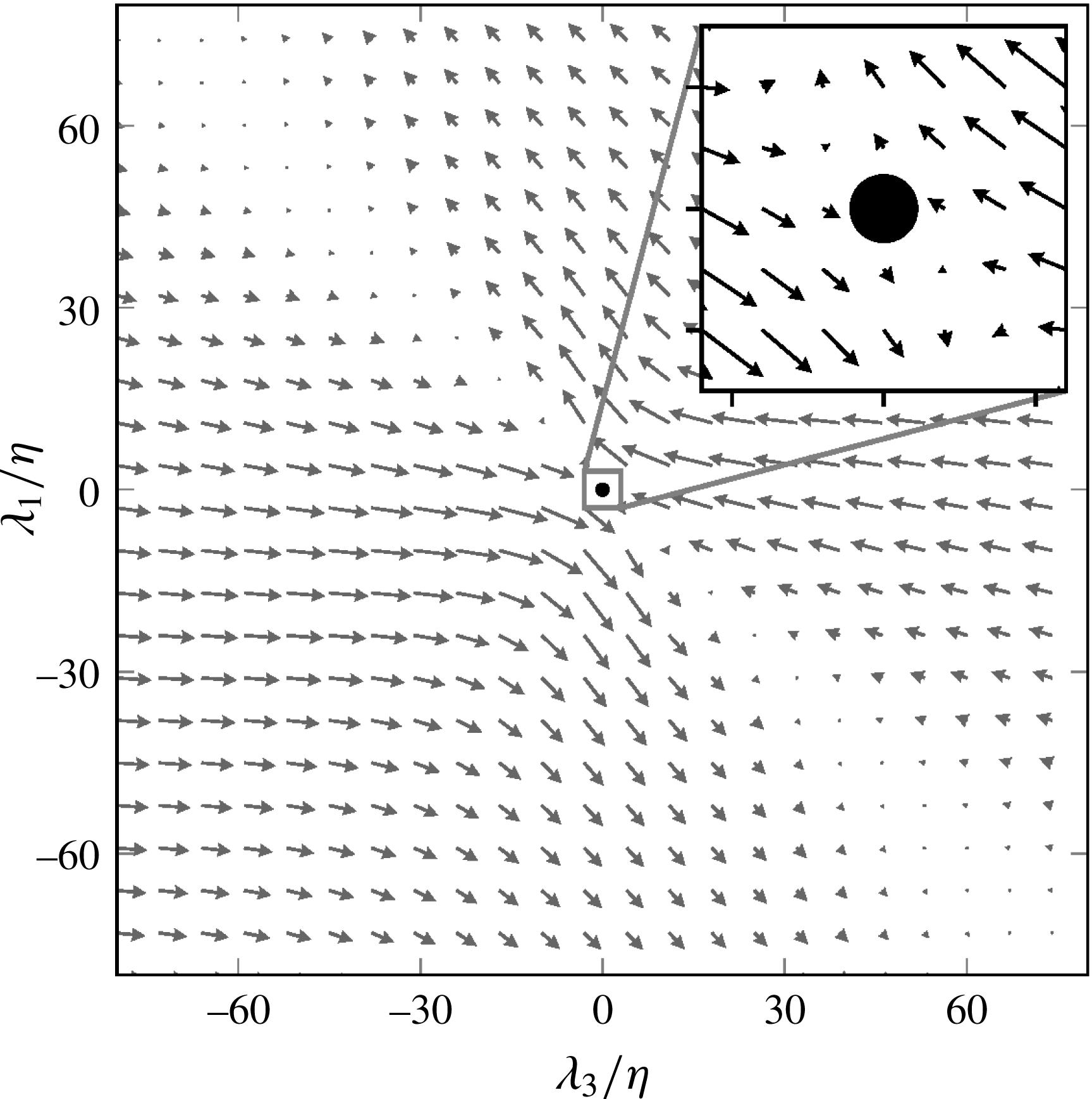
Burgers vortex in a Cartesian coordinate system. (a, b) Represent velocity vector plots in
 $\unicode[STIX]{x1D706}_{1}=0$
, and
 $\unicode[STIX]{x1D706}_{2}=0$
,
 $\unicode[STIX]{x1D706}_{3}=0$
planes, respectively. All length scales are normalised by the Kolmogorov length scale (
 $\unicode[STIX]{x1D702}$
).

Figure 1 illustrates the Burgers vortex computed from (2.1) using the above mentioned values. All the length and velocities scales are converted from the cylindrical to a Cartesian coordinate system (
 $\unicode[STIX]{x1D706}_{1},\unicode[STIX]{x1D706}_{2},\unicode[STIX]{x1D706}_{3}$
) to simplify the comparison between different structures. Here
 $\unicode[STIX]{x1D706}_{2}$
and
 $\unicode[STIX]{x1D706}_{3}$
are radial/compressive strain directions and
 $\unicode[STIX]{x1D706}_{1}$
corresponds to the stretching strain direction, which coincides with the vortex axis, i.e. the
 $z$
-axis in (2.1). Figure 1(a) shows the swirling flow in the plane perpendicular to the vortex axis (
 $\unicode[STIX]{x1D706}_{1}$
direction), while figure 1(b) illustrates the stretching motion along the vortex axis, and compression along the radial directions (
 $\unicode[STIX]{x1D706}_{2}$
and
 $\unicode[STIX]{x1D706}_{3}$
).
2.2 Shear-layer structure (SLS)
The shear-layer structure (SLS) is extracted from a direct numerical simulation (DNS) of homogeneous isotropic turbulence (Li et al.
Reference Li, Perlman, Wan, Yang, Meneveau, Burns, Chen, Szalay and Eyink2008) at a Taylor Reynolds number
 $Re_{\unicode[STIX]{x1D706}}=433$
using the averaging procedure described in Elsinga & Marusic (Reference Elsinga and Marusic2010). Basically, this structure describes the average flow around a point when the observer is aligned with the local directions of principal strain. The SLS appeared qualitatively similar in different kinds of turbulent flows, as such, it is considered universal (Elsinga & Marusic Reference Elsinga and Marusic2010). For homogeneous isotropic turbulence at
 $Re_{\unicode[STIX]{x1D706}}>250$
, it was shown that the velocity within
 $60\unicode[STIX]{x1D702}$
distance from the origin of the SLS is independent of the Reynolds number when using Kolmogorov scaling (Elsinga & Marusic Reference Elsinga and Marusic2016). Furthermore, there exists an approximate balance between vorticity stretching and diffusion within the core of the shear layer, which causes the material derivative of vorticity to be small when compared to the peak vorticity magnitude squared (
 $O(10^{-2})$
(Elsinga & Marusic Reference Elsinga and Marusic2016)). This means that the SLS evolves slowly, which is consistent with the concept of coherent structures (see introduction). A brief explanation of the averaging procedure to extract this structure is as follows.
First, the strain-rate tensor is computed from the velocity gradients (
 $\unicode[STIX]{x2202}u_{i}/\unicode[STIX]{x2202}x_{j}$
) at a point
 $\boldsymbol{x}_{p}$
in the turbulent flow database. Then, the eigenvalues and the principal directions (i.e. eigenvectors) of the strain-rate tensor are calculated. The principal directions
 $\boldsymbol{e}_{1},\boldsymbol{e}_{2}$
and
 $\boldsymbol{e}_{3}$
represent the most stretching, the intermediate and the most compressing straining directions, respectively. Furthermore, the positive intermediate straining direction (
 $\boldsymbol{e}_{2}$
) is chosen such that its dot product with the vorticity vector is positive. The vector
 $\boldsymbol{e}_{3}$
is fixed as the third direction. To complete the right-handed coordinate system, the first direction (
 $\boldsymbol{e}_{1}$
) is computed as the cross-product between
 $\boldsymbol{e}_{2}$
and
 $\boldsymbol{e}_{3}$
. Then the new coordinate system (
 $\unicode[STIX]{x1D706}_{i}$
) is defined along the corresponding principal directions
 $\boldsymbol{e}_{i}$
. The flow velocities (
 $\boldsymbol{u}$
) on the new grid (
 $\unicode[STIX]{x1D706}_{1},\unicode[STIX]{x1D706}_{2},\unicode[STIX]{x1D706}_{3}$
) relative to the point
 $\boldsymbol{x}_{p}$
are computed by linear interpolation, where the grid spacing is one Kolmogorov length scale in each direction. The components
 $u_{i}$
represent velocities along the corresponding
 $\unicode[STIX]{x1D706}_{i}$
directions. This three-dimensional velocity field in the new local coordinate system is then calculated for different points
 $\boldsymbol{x}_{p}$
in the flow and finally averaged over all points
 $\boldsymbol{x}_{p}$
considered. The result is the shear-layer structure illustrated in figure 2. One of the main features of this structure can be observed in figure 2(b), where the shear layer spans from the top left corner in figure to the bottom right corner. Figures 2(a) and 2(c) represent the velocity in the cross-planes
 $\unicode[STIX]{x1D706}_{1}=0$
and
 $\unicode[STIX]{x1D706}_{3}=0$
, respectively, where the flow is compressive along the
 $\unicode[STIX]{x1D706}_{3}$
direction and stretching along the intermediate straining direction
 $\unicode[STIX]{x1D706}_{2}$
and along
 $\unicode[STIX]{x1D706}_{1}$
. This leads to a saddle topology at the origin in figure 2(a) and a node in figure 2(c).
Shear-layer structure extracted from the isotropic turbulent flow (Li et al.
Reference Li, Perlman, Wan, Yang, Meneveau, Burns, Chen, Szalay and Eyink2008) at
 $Re_{\unicode[STIX]{x1D706}}=433$
. (a–c) Represent velocity vector plots in the cross-planes
 $\unicode[STIX]{x1D706}_{1}=0$
,
 $\unicode[STIX]{x1D706}_{2}=0$
and
 $\unicode[STIX]{x1D706}_{3}=0$
, respectively. (d) Illustrates the streamlines in
 $\unicode[STIX]{x1D706}_{2}=0$
cross-plane. All the length scales are normalised by the Kolmogorov length scale (
 $\unicode[STIX]{x1D702}$
).

2.3 Node-saddle topology
The node-saddle topology (NST) is obtained by applying planar symmetry to all velocities (
 $u_{1},u_{2},u_{3}$
) in the previously discussed shear-layer structure. The velocity component
 $u_{1}$
is made symmetric about the plane
 $\unicode[STIX]{x1D706}_{1}=0$
. Similarly,
 $u_{2}$
and
 $u_{3}$
are made symmetric about the planes
 $\unicode[STIX]{x1D706}_{2}=0$
and
 $\unicode[STIX]{x1D706}_{3}=0$
, respectively. This symmetric operation maintains the strain of the shear-layer structure and removes its vorticity. The velocity vectors in the different cross-planes are shown in figure 3. The difference between the node-saddle topology and the shear-layer structure can be seen by comparing figures 2 and 3. The shear layer in figure 2(b) vanishes in figure 3(b) due to the planar symmetry, resulting in a pure node-saddle critical point with no vorticity at the origin. As before, the flow in the other cross-planes shows a saddle (figure 3
a) and a node topology at the origin (figure 3
c).
Node-saddle topology obtained by symmetrising the shear-layer structure presented in figure 2. (a–c) Represent velocity vector plots in the cross-planes
 $\unicode[STIX]{x1D706}_{1}=0$
,
 $\unicode[STIX]{x1D706}_{2}=0$
and
 $\unicode[STIX]{x1D706}_{3}=0$
, respectively. (d) Illustrates the streamlines in the
 $\unicode[STIX]{x1D706}_{2}=0$
cross-plane. All the length scales are normalised by the Kolmogorov length scale (
 $\unicode[STIX]{x1D702}$
).

3 Particle simulation and statistics
The point particles considered in the pair and tetrad dispersion are passive tracers or marked fluid parcels. Their motion is simulated according to
 $$\begin{eqnarray}\frac{\text{d}\boldsymbol{x}_{p}(t)}{\text{d}t}=\boldsymbol{u}(\boldsymbol{x}_{p}(t)),\end{eqnarray}$$
where
 $\boldsymbol{u}(\boldsymbol{x}_{p})$
represents the fluid velocity at the instantaneous particle position
 $\boldsymbol{x}_{p}$
. The explicit fourth-order Runge–Kutta scheme is employed to integrate the equation in time. The velocity on the right-hand side is calculated by the tri-linear interpolation of the velocity field of the shear-layer structure and the node-saddle topology. For the Burgers vortex, the equations (2.1) are used to compute velocity at the particle position. To study pair dispersion, 5000 particle pairs are initially uniformly distributed on a sphere around the origin (Saff & Kuijlaars Reference Saff and Kuijlaars1997), where the centre of the mass of each pair coincides with the origin of the extracted flow structures, as shown in figure 4. The particle distribution is chosen around the origin of the structures, which correspond to critical points. These critical points have a notable effect on the particle dispersion as discussed in the introduction. Subsequently, the particle motion follows from the above equation. Due to the symmetries in the considered flow structures the centre of the mass of a particle pair remains at the origin in all cases and at all times. The initial separation distance between the two particles of a pair is defined as the diameter of the sphere, i.e. twice the distance between the particle and the origin, where the centre of the mass of the pair is located. Similar to the pair dispersion, tetrad dispersion is studied by kinematically simulating 4000 regular tetrahedrons (same edge length) around the origin of the flow structures. The origin of the structure coincides with the centroid of the tetrahedron. The quantities to describe the pair and tetrad dispersion are explained in §§ 3.1 and 3.3, respectively. The details concerning the simulations of material lines and the statistics of their orientation will be discussed in § 3.2.
Projection of 5000 particles on the
 $\unicode[STIX]{x1D706}_{2}=0$
plane at time
 $t=0$
. The particles are distributed on the surface of a sphere centred at the origin of the shear-layer structure with initial separation
 $|\boldsymbol{r}_{0}|=\unicode[STIX]{x1D702}$
. The projection of particles onto a plane leads to the overlapping of particles to form a circle.
3.1 Pair dispersion
The pair dispersion describes the average separation of particles. This is characterised by the evolution of the mean square of the relative separation (MSRS) between two particles (Richardson Reference Richardson1926; Batchelor Reference Batchelor1950), which is expressed as
 $\langle |\boldsymbol{r}(t)-\boldsymbol{r}(0)|^{2}\rangle$
, where
 $\boldsymbol{r}(t)$
represents the separation vector at time
 $t$
,
 $\boldsymbol{r}(0)$
is the initial separation vector and
 $\langle \cdot \rangle$
and
 $|\cdot |$
describe the mean and the Euclidean norm, respectively. The separation vector
 $\boldsymbol{r}(t)$
is computed as
 $\boldsymbol{x}_{1}(t)-\boldsymbol{x}_{2}(t)$
, where
 $\boldsymbol{x}_{1}(t)$
and
 $\boldsymbol{x}_{2}(t)$
are the positions of the two particles at time
 $t$
. In the inertial range of the turbulent flow, Batchelor (Reference Batchelor1950) predicted the mean square of the relative separation as
 $$\begin{eqnarray}\langle |\boldsymbol{r}(t)-\boldsymbol{r}(0)|^{2}\rangle =\left\{\begin{array}{@{}ll@{}}\frac{11}{3}C_{2}(\unicode[STIX]{x1D716}r_{0})^{2/3}t^{2}\quad & \text{for }t\ll t_{B}=r_{0}^{2/3}\langle \unicode[STIX]{x1D716}\rangle ^{-1/3}\\ \frac{3}{2}g\,\unicode[STIX]{x1D716}\,t^{3}\quad & \text{for }t_{B}\ll t\ll T_{L},\end{array}\right.\end{eqnarray}$$
where
 $C_{2}$
is the Kolmogorov constant in the second-order Eulerian structure function,
 $\unicode[STIX]{x1D716}$
is the average dissipation rate of the flow,
 $r_{0}$
is the initial separation between the particle pair,
 $t_{B}$
is Batchelor’s time scale after which dispersion is not influenced by
 $r_{0}$
,
 $g$
is Richardson’s constant, which is assumed to be a fundamental constant in turbulence, and
 $T_{L}$
is the integral time scale of the flow. The first sub-range where
 $t\ll t_{B}$
(see (3.2)) is referred to as Batchelor’s ballistic regime or Batchelor’s scaling. In the literature,
 $t_{B}$
is considered as the time where the two particles remain within the same structure of size
 $r_{0}$
. When the particles leave the structure, i.e. at times
 $t\gg t_{B}$
, the particle separation is supposed to transition into Richardson’s
 $t^{3}$
scaling (see (3.2)). However, Bitane et al. (Reference Bitane, Homann and Bec2012) have shown that Richardson’s scaling regime follows directly after Batchelor’s scaling (see also § 4.3).
The mean square of the relative separation is computed for different initial separations in each structure. Then, the existence of the Batchelor ballistic regime and a Richardson scaling regime is probed. Finally, the compensated relative dispersion results are compared with the data from actual turbulence (Sawford et al. Reference Sawford, Yeung and Hackl2008) in § 4.1.
3.2 Material lines
A material line is an infinitesimal line composed of the same fluid particles when evolved in time, hence studying their orientation aids in the understanding of turbulence mixing (Batchelor Reference Batchelor1952b ). Here, the evolution of the orientation of the material lines is examined to understand the differences between different structures. Furthermore, the results are compared with the actual turbulent flow (Guala et al. Reference Guala, Liberzon, Lüthi, Kinzelbach and Tsinober2006). Material lines evolve with time according to (Girimaji & Pope Reference Girimaji and Pope1990; Dresselhaus & Tabor Reference Dresselhaus and Tabor1992; Guala et al. Reference Guala, Liberzon, Lüthi, Kinzelbach and Tsinober2006):
 $$\begin{eqnarray}\frac{\text{d}l_{i}(t)}{\text{d}t}=\frac{\unicode[STIX]{x2202}u_{i}}{\unicode[STIX]{x2202}x_{j}}l_{j}(t),\end{eqnarray}$$
where
 $l_{i}$
represents the infinitesimal material line,
 $\unicode[STIX]{x2202}u_{i}/\unicode[STIX]{x2202}x_{j}$
refers to the velocity gradient tensor computed at the centre of
 $l_{i}$
. In the present study, material lines are assumed to continuously evolve around the origin, as the flow structures are stationary and the velocity at the origin is zero. This implies that the initially placed infinitesimal line elements at the origin do not advect, but reorient according to the same stationary velocity gradient tensor. Hence, the velocity gradient in (3.3) is constant in time and is computed at the origin of each flow structure. The alignment of the material lines with the straining directions is given by
 $\cos (\boldsymbol{l},\boldsymbol{e}_{i})=(\boldsymbol{l}\boldsymbol{\cdot }\boldsymbol{e}_{i})/(|\boldsymbol{l}||\boldsymbol{e}_{i}|)$
, where
 $\boldsymbol{e}_{i}$
represents the eigenvectors of the strain-rate tensor at the origin of the structure. A total of
 $10^{4}$
material lines are considered in the present study, and their alignment for all structures is compared in § 4.4 with the data presented by Guala et al. (Reference Guala, Liberzon, Lüthi, Kinzelbach and Tsinober2006).
3.3 Four-particle dispersion
The tetrad dispersion is quantified by the evolution of its size and shape, which are based on the separation between the different particles in the tetrahedron. The procedure to characterise the size and shape of the tetrahedron is similar to Biferale et al. (Reference Biferale, Boffetta, Celani, Devenish, Lanotte and Toschi2005). At first, the coordinates are changed to obtain a new set of separation vectors (Chertkov et al.
Reference Chertkov, Pumir and Shraiman1999; Biferale et al.
Reference Biferale, Boffetta, Celani, Devenish, Lanotte and Toschi2005; Hackl et al.
Reference Hackl, Yeung and Sawford2011), which eliminates the statistical dependence on the centre of mass
 $\boldsymbol{X}_{0}$
, where
 $\boldsymbol{X}_{0}=(\boldsymbol{x}_{1}+\boldsymbol{x}_{2}+\boldsymbol{x}_{3}+\boldsymbol{x}_{4})/4$
and
 $\boldsymbol{x}_{i}$
represent the particle positions in the tetrahedron. Note that the centre of mass
 $\boldsymbol{X}_{0}$
coincides with the origin of the structure initially. The three separation vectors are defined as (Chertkov et al.
Reference Chertkov, Pumir and Shraiman1999; Biferale et al.
Reference Biferale, Boffetta, Celani, Devenish, Lanotte and Toschi2005; Hackl et al.
Reference Hackl, Yeung and Sawford2011)
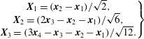 $$\begin{eqnarray}\left.\begin{array}{@{}c@{}}\boldsymbol{X}_{1}=(\boldsymbol{x}_{2}-\boldsymbol{x}_{1})/\sqrt{2},\\ \boldsymbol{X}_{2}=(2\boldsymbol{x}_{3}-\boldsymbol{x}_{2}-\boldsymbol{x}_{1})/\sqrt{6},\\ \boldsymbol{X}_{3}=(3\boldsymbol{x}_{4}-\boldsymbol{x}_{3}-\boldsymbol{x}_{2}-\boldsymbol{x}_{1})/\sqrt{12}.\end{array}\right\}\end{eqnarray}$$
Then, an inertia matrix (
 $\unicode[STIX]{x1D644}$
) is computed as
 $\unicode[STIX]{x1D644}=\unicode[STIX]{x1D746}\unicode[STIX]{x1D746}^{\text{T}}$
where the columns of the matrix
 $\unicode[STIX]{x1D746}$
are the separation vectors (
 $\boldsymbol{X}_{1},\boldsymbol{X}_{2},\boldsymbol{X}_{3}$
). Then the shape and size of the tetrahedron are described by the three eigenvalues (
 $g_{i}$
) of the inertia matrix, where
 $g_{1}\geqslant g_{2}\geqslant g_{3}$
. The size of the tetrahedron is given by the gyration radius
 $R\equiv \sqrt{Tr(\unicode[STIX]{x1D644})}=\sqrt{\sum g_{i}}$
and the tetrahedron volume (
 $V$
) is defined as
 $V=(1/3)\det (\unicode[STIX]{x1D746})=(1/3)\sqrt{g_{1}g_{2}g_{3}}$
. And finally, the shapes are characterised by
 $S_{i}=g_{i}/R^{2}$
, where
 $S_{i}=1/3$
for
 $i=1,2$
and
 $3$
for a regular tetrahedron. If all four points are coplanar then
 $S_{3}=0$
and if collinear
 $S_{2}=S_{3}=0$
.
The evolution of the shape and the size of the tetrahedrons around the structures is computed in terms of the eigenvalues
 $g_{i}$
and compared to the actual turbulence cases (Biferale et al.
Reference Biferale, Boffetta, Celani, Devenish, Lanotte and Toschi2005; Hackl et al.
Reference Hackl, Yeung and Sawford2011) in § 4.5.
4 Results
The dispersion statistics are investigated by kinematically simulating the tracer particles around different structures, namely the shear-layer structure (SLS), the node-saddle topology (NST) and the Burgers vortex (BV) as explained in §§ 2 and 3. The number of particle pairs (
 $5000$
), material lines (
 $10^{4}$
) and tetrahedrons (
 $4000$
) investigated are fewer, but sufficient to obtain converged statistics, compared to the actual turbulent studies, where, the number is usually above
 $10^{5}$
. The statistics are considered converged if the convergence rate is below
 $10^{-4}$
. Here, the convergence rate is defined as the change in statistical value with respect to the increase in the number of particle pairs or material lines or tetrahedrons.
In the following paragraphs, first the pair dispersion statistics around the different structures are examined to determine the Batchelor scaling range. Second, the pair dispersion statistics are compared to the actual turbulent flows. Third, the instantaneous distribution of particles is discussed and related to the observed pair dispersion scaling regimes. Finally the advanced dispersion statistics, namely the orientation of material lines and the tetrad dispersion, are studied and compared with the actual turbulent flow statistics.
4.1 Pair dispersion
The pair dispersion is quantified in terms of the evolution of the mean square of the relative separation (MSRS)
 $\langle |\boldsymbol{r}(t)-\boldsymbol{r}(0)|^{2}\rangle$
. A comparison of the MSRS for the three different structures and for initial separations
 $r_{0}/\unicode[STIX]{x1D702}=1,4$
and 16 is shown in figure 5. The relative separation and time (
 $t$
) are normalised by the Kolmogorov length (
 $\unicode[STIX]{x1D702}$
) and time scale (
 $\unicode[STIX]{x1D70F}_{\unicode[STIX]{x1D702}}$
), respectively. Qualitatively, similar slopes are observed for the MSRS for the Burgers vortex, the shear-layer structure and the node-saddle topology for time
 $t/\unicode[STIX]{x1D70F}_{\unicode[STIX]{x1D702}}<1$
and for all initial separations considered (see figure 5). However, quantitatively the relative separation for the Burgers vortex is higher compared to the SLS and the NST. This is because the BV is based on intense vortices, where velocities and their gradients are higher compared to the SLS and the NST, which are average structures. For time
 $t/\unicode[STIX]{x1D70F}_{\unicode[STIX]{x1D702}}>1$
, the MSRS increases smoothly for the SLS and the NST. However, for the Burgers vortex the MSRS shows an oscillatory behaviour before it increases rapidly at later times. This oscillatory behaviour is due to the circular motion of the particles in the BV, which results in the particles approaching their initial position after every revolution. With time the oscillation fades, as the particles approach the vortex core and the stretching in the axial direction starts to dominate the particle separation. It is also noted that the statistics for the SLS and the NST are found to be approximately similar for all initial separations until
 $t/\unicode[STIX]{x1D70F}_{\unicode[STIX]{x1D702}}=20$
.
The comparison of the evolution of the mean square of relative separation, normalised by the Kolmogorov length (
 $\unicode[STIX]{x1D702}$
), for different structures and for different initial separations (
 $r_{0}/\unicode[STIX]{x1D702}=1,4$
and 16). Time
 $t$
is normalised by the Kolmogorov time scale (
 $\unicode[STIX]{x1D70F}_{\unicode[STIX]{x1D702}}$
). The straight black dotted line corresponds to Batchelor’s
 $t^{2}$
scaling and the dashed line to Richardson’s
 $t^{3}$
scaling. Dashed-dotted lines refer to the Burgers vortex, solid lines to the shear-layer structure and lines with ‘
 $+$
’ mark the node-saddle topology (NST).

The Batchelor scaling is represented by the
 $t^{2}$
curve in figure 5. In the Burgers vortex case, the relative separation scales with
 $t^{2}$
for time
 $t/\unicode[STIX]{x1D70F}_{\unicode[STIX]{x1D702}}<1$
. For the SLS and the NST, the
 $t^{2}$
scaling is observed until
 $t/\unicode[STIX]{x1D70F}_{\unicode[STIX]{x1D702}}\approx 3{-}4$
for the initial separations
 $r_{0}/\unicode[STIX]{x1D702}=1$
and 4. This time scale is consistent with the results in actual turbulence by Sawford et al. (Reference Sawford, Yeung and Hackl2008) and figure 1 of Bitane et al. (Reference Bitane, Homann and Bec2012). For
 $r_{0}/\unicode[STIX]{x1D702}=16$
, Batchelor’s regime is observed for a longer time, up to
 $t/\unicode[STIX]{x1D70F}_{\unicode[STIX]{x1D702}}\approx 9{-}10$
. Approximate Richardson
 $t^{3}$
scaling is observed for
 $r_{0}/\unicode[STIX]{x1D702}\leqslant 4$
for short times in the SLS and the NST. This will be discussed in more detail in § 4.3. However, there is no evidence of Richardson’s regime in the Burgers vortex. From all these observations, it is deduced that Batchelor’s regime, where particles are influenced by their initial separation, is observed in the all three flow structures, as expected. However, the statistics around the Burgers vortex quantitatively and qualitatively differ from the SLS and the NST after time
 $t/\unicode[STIX]{x1D70F}_{\unicode[STIX]{x1D702}}=1$
.
Furthermore, the dispersion around the shear-layer structure and the node-saddle topology is compared to actual homogeneous isotropic turbulence at Taylor Reynolds number
 $Re_{\unicode[STIX]{x1D706}}=650$
(Sawford et al.
Reference Sawford, Yeung and Hackl2008). The evolution of the compensated relative dispersion (
 $\langle \boldsymbol{r}(t)^{2}-\boldsymbol{r}(0)^{2}\rangle /\unicode[STIX]{x1D716}t^{3}$
) with time is shown in figure 6. Here, the dissipation
 $\unicode[STIX]{x1D716}$
is taken from the same database employed to extract structures (Li et al.
Reference Li, Perlman, Wan, Yang, Meneveau, Burns, Chen, Szalay and Eyink2008). The initial separations investigated are
 $r_{0}/\unicode[STIX]{x1D702}=1,4$
and 16.
Comparison of the compensated relative dispersion for the shear-layer structure, node-saddle topology and actual isotropic turbulence (from Sawford et al. (Reference Sawford, Yeung and Hackl2008)). Results are shown for initial separation distances
 $r_{0}=1\unicode[STIX]{x1D702},4\unicode[STIX]{x1D702}$
and
 $16\unicode[STIX]{x1D702}$
.

The compensated relative dispersion (figure 6) in the actual turbulence case and the SLS collapse onto each other until the time
 $t/\unicode[STIX]{x1D70F}_{\unicode[STIX]{x1D702}}=20$
for the initial separation
 $1\unicode[STIX]{x1D702}$
and until time
 $10\unicode[STIX]{x1D70F}_{\unicode[STIX]{x1D702}}$
for
 $r_{0}/\unicode[STIX]{x1D702}=4$
and 16. In the case of the node-saddle topology, the compensated relative dispersion is similar to the actual turbulence case until 4–
 $5\unicode[STIX]{x1D70F}_{\unicode[STIX]{x1D702}}$
for initial separations
 $r_{0}/\unicode[STIX]{x1D702}=1$
and 4. For
 $r_{0}/\unicode[STIX]{x1D702}=16$
, the NST shows a similar trend as the SLS. Also, it can be observed that, qualitatively, the SLS is closer to actual turbulence until
 $t/\unicode[STIX]{x1D70F}_{\unicode[STIX]{x1D702}}\approx 20$
than the NST for
 $r_{0}/\unicode[STIX]{x1D702}=1$
and 4. During the time
 $t/\unicode[STIX]{x1D70F}_{\unicode[STIX]{x1D702}}\approx 30{-}100$
, the compensated relative dispersion for different initial separations in the actual turbulence case undergoes transition and attains a plateau. This plateau indicates Richardson’s regime (Sawford et al.
Reference Sawford, Yeung and Hackl2008) and the value of the compensated relative dispersion is equal to the Richardson constant (
 $g\approx 0.6$
, see (3.2)). However, for
 $r_{o}=16\unicode[STIX]{x1D702}$
the scaling in the SLS and the NST changes to the diffusive regime, where the mean-square separation of the particles scales with
 $t$
. Additionally, the qualitative trend of the transition from
 $t^{2}$
to the point where the curves for the initial separations
 $\unicode[STIX]{x1D702}$
and
 $4\unicode[STIX]{x1D702}$
approach each other is similar to actual turbulence, but much shorter. The transition occurs at
 $t/\unicode[STIX]{x1D70F}_{\unicode[STIX]{x1D702}}\approx 3{-}13$
in the case of the SLS and the NST compared to
 $t/\unicode[STIX]{x1D70F}_{\unicode[STIX]{x1D702}}\approx 3{-}40$
for actual turbulence (Sawford et al.
Reference Sawford, Yeung and Hackl2008). This quantitative difference could be due the absence of additional structures in the SLS and the NST, which is consistent with Batchelor’s conjecture that the particles enter different structures when the scaling changes from the Batchelor regime to the Richardson regime.
From all these observations, it is understood that the shear-layer structure and the node-saddle topology have quantitatively similar pair dispersion statistics to the actual turbulent flow up to
 $t/\unicode[STIX]{x1D70F}_{\unicode[STIX]{x1D702}}\approx 3{-}10$
, which corresponds to Batchelor’s regime. Additionally, the SLS is observed to follow the actual turbulence more closely than the NST until
 $t/\unicode[STIX]{x1D70F}_{\unicode[STIX]{x1D702}}\approx 20$
.
4.2 Instantaneous distribution of particles
Evolution of 5000 particles in the shear-layer structure with time (columns) projected on three different planes (rows). Initially, the particles are distributed on a sphere with a radius of
 $0.5\unicode[STIX]{x1D702}$
, which corresponds to an initial pair separation of
 $1\unicode[STIX]{x1D702}$
. Columns from left to right show the resulting particle distributions at times
 $t/\unicode[STIX]{x1D70F}_{\unicode[STIX]{x1D702}}=4,10$
and 50. The projections of the 5000 particles overlap, and therefore initially appear as one ellipsoid.

Evolution of 5000 particles in the node-saddle topology with time (columns) projected on three different planes (rows). Initially, the particles are distributed on a sphere with a radius of
 $0.5\unicode[STIX]{x1D702}$
, which corresponds to an initial pair separation of
 $1\unicode[STIX]{x1D702}$
. Columns from left to right show the resulting particle distributions at times
 $t/\unicode[STIX]{x1D70F}_{\unicode[STIX]{x1D702}}=4,10$
and 50. The projections of the 5000 particles overlap, and therefore initially appear as one ellipsoid.

(a–d) Distribution of particles in the shear-layer structure projected on the plane
 $\unicode[STIX]{x1D706}_{2}=0$
at times
 $t/\unicode[STIX]{x1D70F}_{\unicode[STIX]{x1D702}}=4,8,10$
and 25, respectively. The initial pair separation is
 $1\unicode[STIX]{x1D702}$
. With time, the particles align themselves along the shear layer, forming a sheet.

While the relative dispersion of particles by the SLS and the NST is qualitatively similar, the underlying particle distribution in physical space appears to be different, which is illustrated in this section. The distribution of particles in time for the initial separation distance
 $r_{0}/\unicode[STIX]{x1D702}=1$
is shown for the SLS and the NST in figures 7 and 8, respectively. The three rows of plots in these figures represent the projections on the three Cartesian planes, namely
 $\unicode[STIX]{x1D706}_{3}=0,~\unicode[STIX]{x1D706}_{2}=0$
and
 $\unicode[STIX]{x1D706}_{1}=0$
from top to bottom. The three columns from left to right show the time evolution of particles at times
 $t/\unicode[STIX]{x1D70F}_{\unicode[STIX]{x1D702}}=4,10$
, and 50, respectively.
The first rows in figures 7 and 8 show the particle distribution on the plane spanned by the extensive principal straining directions
 $\unicode[STIX]{x1D706}_{1}$
and
 $\unicode[STIX]{x1D706}_{2}$
for the SLS and the NST, respectively. Initially at
 $t/\unicode[STIX]{x1D70F}_{\unicode[STIX]{x1D702}}=0$
, the particles are distributed on a sphere leading to the circular distribution in the projections (see figure 4). With time, the projected distribution of particles develops an ellipsoidal shape due to the higher rate of stretching in the
 $\unicode[STIX]{x1D706}_{1}$
direction compared to the intermediate principal straining direction,
 $\unicode[STIX]{x1D706}_{2}$
(
 $t/\unicode[STIX]{x1D70F}_{\unicode[STIX]{x1D702}}=4$
and 10). Furthermore, the size of the ellipse increases, because the stretching rate in both directions is positive. At later times, the ellipsoid splits into two (e.g. at
 $t/\unicode[STIX]{x1D70F}_{\unicode[STIX]{x1D702}}=50$
).
The second row in figure 7 corresponds to the particle distribution on the plane with the most extensive and the compression principal strain rates. The particle distribution gets stretched along the shear layer (see figure 9 for the associated velocity vectors) with increasing time. In this projection, the particles are distributed along a line, which is at an
 $18^{^{\circ }}$
angle with respect to the direction of the most stretching principle strain
 $\unicode[STIX]{x1D706}_{1}$
at
 $t/\unicode[STIX]{x1D70F}_{\unicode[STIX]{x1D702}}=4$
(see figure 7
d). At later time
 $t/\unicode[STIX]{x1D70F}_{\unicode[STIX]{x1D702}}=50$
, the projected particle distribution approaches the
 $45^{^{\circ }}$
diagonal (figure 7
f). However for the NST, the particles on the same plane are stretched along the
 $\unicode[STIX]{x1D706}_{1}$
and compressed in the
 $\unicode[STIX]{x1D706}_{3}$
direction (figure 8). This is attributed to the absence of rotation/vorticity in the node-saddle topology. The NST particle distribution essentially forms a line in the
 $\unicode[STIX]{x1D706}_{1}$
direction, as observed in figure 8(d–f).
The distribution of particles for the SLS and the NST is also different in the
 $\unicode[STIX]{x1D706}_{1}=0$
plane, which is shown in the third row of figures 7 and 8, respectively. The difference is again attributed to the presence of rotation in the shear layer. Due to the rotation, the particles get distributed along the shear layer, thereby, actually spreading the particles in the direction of compressive strain (
 $\unicode[STIX]{x1D706}_{3}$
). However, the absence of rotation in the NST causes the particles to collapse onto a line along the
 $\unicode[STIX]{x1D706}_{2}$
axis at time
 $t/\unicode[STIX]{x1D70F}_{\unicode[STIX]{x1D702}}=50$
(see figure 8
g–i).
From these observations, it is concluded that the particles in the node-saddle topology at
 $t/\unicode[STIX]{x1D70F}_{\unicode[STIX]{x1D702}}>10$
form a sheet spanning the
 $\unicode[STIX]{x1D706}_{1}$
and
 $\unicode[STIX]{x1D706}_{2}$
directions. In contrast, the particle sheet in the shear-layer structure is at an angle with the
 $\unicode[STIX]{x1D706}_{1}$
and
 $\unicode[STIX]{x1D706}_{3}$
directions, while it is still aligned with the
 $\unicode[STIX]{x1D706}_{2}$
direction. Hence, the particles actually spread in the direction of the most compressive strain
 $\unicode[STIX]{x1D706}_{3}$
. The pair dispersion statistics i.e. the mean square of relative separation, of the NST and the SLS are found to be similar even though the particles in the node-saddle topology do not move away from the origin in the compression direction. However, the observed differences in particle sheet formation are important when considering the orientation of material lines and the geometry of four-particle dispersion in § 4.4 and § 4.5, respectively.
4.3 A comment on pair dispersion scaling
Besides the sheet forming characteristics, the particle distributions in § 4.2 also provide important insights in the pair dispersion scaling regimes. The mean-square relative separation scales according to
 $t^{2}$
until
 $t/\unicode[STIX]{x1D70F}_{\unicode[STIX]{x1D702}}\approx 3$
–
 $4$
(§ 4.1), which is associated with Batchelor’s ballistic regime where the particle velocity is assumed constant. However, the particle distributions reveal that the particles have moved significantly towards the end of the observed
 $t^{2}$
scaling range. For example, figure 7(d) shows that at
 $t/\unicode[STIX]{x1D70F}_{\unicode[STIX]{x1D702}}=4$
some particles have approached the origin, where the velocity goes to zero, while others have reached distances as large as
 $2\unicode[STIX]{x1D702}$
away from the origin, thereby significantly increasing their velocity. Up to
 $5\unicode[STIX]{x1D702}$
distance from the origin of the SLS and the NST, the velocity varies approximately linearly with distance (see Elsinga et al.
Reference Elsinga, Ishihara, Goudar, da Silva and Hunt2017), which means that at
 $2\unicode[STIX]{x1D702}$
distance from the origin the particle velocity has increased approximately fourfold from its initial value when released at
 $0.5\unicode[STIX]{x1D702}$
from the origin. Therefore, the individual particles are subjected to strong changes in their velocity. This point is further illustrated in figure 10, which shows the temporal evolution of the squared separation velocities,
 $|\unicode[STIX]{x1D6FF}\boldsymbol{u}|^{2}(t)$
, for several different pairs. Note that
 $\unicode[STIX]{x1D6FF}\boldsymbol{u}/2$
corresponds to the velocity of the individual particles due to symmetry of the considered flow structures. It is seen that the changes in particle velocity are small only for
 $t$
up to order
 $0.1\unicode[STIX]{x1D70F}_{\unicode[STIX]{x1D702}}$
, which is considered the limit for the true ballistic regime. Thus, while
 $t^{2}$
scaling is observed for
 $0<t/\unicode[STIX]{x1D70F}_{\unicode[STIX]{x1D702}}<4$
, the dispersion is not truly ballistic over most of this range. The original assumptions made when deriving
 $t^{2}$
scaling (Batchelor Reference Batchelor1950) appear to hold only up to
 $t=O(0.1\unicode[STIX]{x1D70F}_{\unicode[STIX]{x1D702}})$
. Then the question remains, why do we still observe
 $t^{2}$
scaling beyond that time scale?
Grey lines indicate the temporal evolution of normalised relative velocity squared for individual particle pairs in the SLS (100 different particle pairs are shown). The thick black line indicates the mean
 $(\langle |\unicode[STIX]{x1D6FF}\boldsymbol{u}|^{2}(t)\rangle -\langle |\unicode[STIX]{x1D6FF}\boldsymbol{u}|^{2}(0)\rangle )/\langle |\unicode[STIX]{x1D6FF}\boldsymbol{u}|^{2}(0)\rangle$
of 5000 particle pairs. Two dashed lines indicate the minimum and maximum limit of the normalised relative velocity squared for 5000 individual particle pairs. The time is normalised by Kolmogorov time scale and the initial separation between the particle pair was
 $1\unicode[STIX]{x1D702}$
.

In order to address this question consider the approximation of the rate of increase of the mean-square relative separation, which was derived through different approaches by Batchelor (Reference Batchelor1950) and Ouellette et al. (Reference Ouellette, Xu, Bourgoin and Bodenschatz2006). It is given by
 $$\begin{eqnarray}\frac{\text{d}\langle |\boldsymbol{r}(t)-\boldsymbol{r}(0)|^{2}\rangle }{\text{d}t}\approx 2t\langle \unicode[STIX]{x1D6FF}\boldsymbol{u}(0)\boldsymbol{\cdot }\unicode[STIX]{x1D6FF}\boldsymbol{u}(0)\rangle\end{eqnarray}$$
and leads to
 $t^{2}$
scaling for
 $\langle |\boldsymbol{r}(t)-\boldsymbol{r}(0)|^{2}\rangle$
. For the above approximation to be valid, it is sufficient that the average
 $\langle |\unicode[STIX]{x1D6FF}\boldsymbol{u}|^{2}\rangle$
is constant as opposed to the ballistic assumption of constant velocity for each particle (see equations (5.1) and (5.2) in Batchelor (Reference Batchelor1950)). The former appears less restrictive, as
 $\langle |\unicode[STIX]{x1D6FF}\boldsymbol{u}|^{2}\rangle$
was observed to be constant up to
 $O(1\unicode[STIX]{x1D70F}_{\unicode[STIX]{x1D702}})$
in actual turbulence for small
 $r_{0}$
(figure 10 and also figure 3 in Bitane et al. (Reference Bitane, Homann and Bec2012)). The averaging compensates decreasing
 $|\unicode[STIX]{x1D6FF}\boldsymbol{u}|^{2}$
associated with compression, i.e. particles approaching each other, with increasing
 $|\unicode[STIX]{x1D6FF}\boldsymbol{u}|^{2}$
associated with stretching, i.e. separating particles. This effect is illustrated using figure 7(d), where all particle pairs are sufficiently close to the origin to assume that their velocity depends linearly on the separation distance,
 $r$
. Some particles have moved closer to the origin, where
 $\unicode[STIX]{x1D6FF}\boldsymbol{u}$
approaches zero, while simultaneously other particles have moved away from the origin increasing the magnitude of
 $\unicode[STIX]{x1D6FF}\boldsymbol{u}$
.
Bitane et al. (Reference Bitane, Homann and Bec2012) considered the scaling transition of
 $\langle |\boldsymbol{r}(t)-\boldsymbol{r}(0)|^{2}\rangle$
and suggested that the Richardson
 $t^{3}$
scaling directly follows the Batchelor
 $t^{2}$
scaling regime. Though Richardson’s scaling was derived for
 $r_{0}$
in the inertial range by Batchelor (Reference Batchelor1950), their results show
 $t^{3}$
scaling only for small initial particle separations,
 $r_{0}\leqslant 4\unicode[STIX]{x1D702}$
, at times of the order of
 $4\unicode[STIX]{x1D70F}_{\unicode[STIX]{x1D702}}$
. Their data for larger
 $r_{0}$
did not extent to sufficiently large times to reach a possible Richardson regime. On the other hand, data from Sawford et al. (Reference Sawford, Yeung and Hackl2008) for similar conditions seem to indicate that the
 $t^{3}$
scaling is approximate (see figure 6). Furthermore, measurements reveal no
 $t^{3}$
scaling for
 $r_{0}$
considerably larger than
 $4\unicode[STIX]{x1D702}$
(see Bourgoin et al.
Reference Bourgoin, Ouellette, Xu, Berg and Bodenschatz2006; Ouellette et al.
Reference Ouellette, Xu, Bourgoin and Bodenschatz2006). Higher Reynolds number flows and data over longer time scales may be needed to address the issue of Richardson scaling in the inertial range. Consistent with the above observations for
 $r_{0}\leqslant 4\unicode[STIX]{x1D702}$
, the mean-square relative separation for the SLS and the NST reveals approximate
 $t^{3}$
scaling for
 $r_{0}=1\unicode[STIX]{x1D702}-4\unicode[STIX]{x1D702}$
and
 $4<t/\unicode[STIX]{x1D70F}_{\unicode[STIX]{x1D702}}<10$
(figure 5). The corresponding particle distributions in figure 7 show that nearly all particles remain within
 $5\unicode[STIX]{x1D702}$
distance from the origin up to
 $t=10\unicode[STIX]{x1D70F}_{\unicode[STIX]{x1D702}}$
, which means
 $r<10\unicode[STIX]{x1D702}$
. The
 $10\unicode[STIX]{x1D702}$
length scale is the typical size for the core of small-scale flow structures, such as the vortices (Jimenez et al.
Reference Jimenez, Wray, Saffman and Rogallo1993) and the straining motions (Elsinga et al.
Reference Elsinga, Ishihara, Goudar, da Silva and Hunt2017), where the velocity varies linearly in space. Therefore, the particle pairs remain within the core of the same small-scale flow structure, while still displaying approximate
 $t^{3}$
scaling. This clearly violates the assumption that particles are far apart, which was used when deriving
 $t^{3}$
scaling (Batchelor Reference Batchelor1950). The same derivation also assumes that the particles are not yet far enough apart for the separation to be affected by energy-containing motions. The latter conflicts with recent observations of intense shear layers, which are small-scale motions bound directly by large-scale energetic motions (Ishihara et al.
Reference Ishihara, Kaneda and Hunt2013; Elsinga et al.
Reference Elsinga, Ishihara, Goudar, da Silva and Hunt2017). Initial separations larger than the layer thickness (
 ${\sim}20\unicode[STIX]{x1D702}$
) are immediately affected by the large-scale motions adjacent to the layer, which could explain why the Richardson scaling is not observed for
 $r_{0}>20\unicode[STIX]{x1D702}$
(Bourgoin et al.
Reference Bourgoin, Ouellette, Xu, Berg and Bodenschatz2006; Ouellette et al.
Reference Ouellette, Xu, Bourgoin and Bodenschatz2006).
Here, we offer an explanation for the observed approximate
 $t^{3}$
scaling for small
 $r_{0}$
based on the observed particle distributions in the SLS (figure 7). However, a similar argument can be constructed using the NST (figure 8). Initially, the particles are located on a sphere of
 $1\unicode[STIX]{x1D702}$
diameter centred on the origin, which represents the case of randomly orientated particle pairs (
 $r_{0}=1\unicode[STIX]{x1D702}$
) with respect to the structure. Therefore, pair statistics can be inferred from the temporal evolution of the particle distribution. The approximate
 $t^{3}$
scaling is observed for
 $4<t/\unicode[STIX]{x1D70F}_{\unicode[STIX]{x1D702}}<10$
. During this time the particles are distributed on a sheet, whose orientation does not change much (figure 7
d,e). Furthermore, the particles remain within the core of the shear layer, where the velocity varies linearly in space, as already mentioned. Based on these observations, we assume that the separation velocity,
 $\unicode[STIX]{x1D6FF}\boldsymbol{u}$
, aligns with the separation vector,
 $\boldsymbol{r}$
, and that they are linearly related according to:
 $\unicode[STIX]{x1D6FF}u_{i}(t)=\text{d}r_{i}(t)/\text{d}t=(\text{d}\unicode[STIX]{x1D6FF}u_{i}/\text{d}r_{i})r_{i}(t)$
with a constant strain rates
 $\text{d}\unicode[STIX]{x1D6FF}u_{i}/\text{d}r_{i}$
. The general solution to the above differential equation is an exponential. The indices
 $i=1$
and
 $2$
in this case refer to the components along the principal stretching directions of the sheet, where the
 $r_{2}$
direction coincides with the
 $\unicode[STIX]{x1D706}_{2}$
direction, while the
 $r_{1}$
direction is at a small angle with respect to the
 $\unicode[STIX]{x1D706}_{1}$
direction (figure 7
d). Furthermore, we define two time scales
 $t_{i}^{\ast }=(\text{d}\unicode[STIX]{x1D6FF}u_{i}/\text{d}r_{i})^{-1}$
. The smallest time scale,
 $t_{1}^{\ast }$
, is representative of the time needed to form the particle sheet, since the compressive strain rate producing the sheet is of similar magnitude as
 $\text{d}\unicode[STIX]{x1D6FF}u_{1}/\text{d}r_{1}$
. Then for the rate of increase of the mean-square relative separation and
 $t>t^{\ast }$
, we find
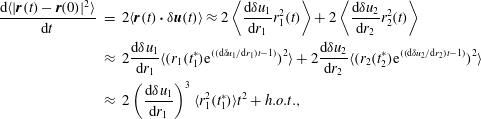 $$\begin{eqnarray}\displaystyle \frac{\text{d}\langle |\boldsymbol{r}(t)-\boldsymbol{r}(0)|^{2}\rangle }{\text{d}t} & = & \displaystyle 2\langle \boldsymbol{r}(t)\boldsymbol{\cdot }\unicode[STIX]{x1D6FF}\boldsymbol{u}(t)\rangle \approx 2\left\langle \frac{\text{d}\unicode[STIX]{x1D6FF}u_{1}}{\text{d}r_{1}}r_{1}^{2}(t)\right\rangle +2\left\langle \frac{\text{d}\unicode[STIX]{x1D6FF}u_{2}}{\text{d}r_{2}}r_{2}^{2}(t)\right\rangle \nonumber\\ \displaystyle & {\approx} & \displaystyle 2\frac{\text{d}\unicode[STIX]{x1D6FF}u_{1}}{\text{d}r_{1}}\langle (r_{1}(t_{1}^{\ast })\text{e}^{((\text{d}\unicode[STIX]{x1D6FF}u_{1}/\text{d}r_{1})t-1)})^{2}\rangle +2\frac{\text{d}\unicode[STIX]{x1D6FF}u_{2}}{\text{d}r_{2}}\langle (r_{2}(t_{2}^{\ast })\text{e}^{((\text{d}\unicode[STIX]{x1D6FF}u_{2}/\text{d}r_{2})t-1)})^{2}\rangle \nonumber\\ \displaystyle & {\approx} & \displaystyle 2\left(\frac{\text{d}\unicode[STIX]{x1D6FF}u_{1}}{\text{d}r_{1}}\right)^{3}\langle r_{1}^{2}(t_{1}^{\ast })\rangle t^{2}+h.o.t.,\end{eqnarray}$$
which leads to initial
 $t^{3}$
scaling for
 $\langle |\boldsymbol{r}(t)-\boldsymbol{r}(0)|^{2}\rangle$
over a short time interval around the sheet formation time
 $t=t_{1}^{\ast }$
. In the last step of (4.2) a Taylor expansion is introduced around
 $t=t^{\ast }$
. Further note that for the SLS and the NST
 $(\text{d}\unicode[STIX]{x1D6FF}u_{1}/\text{d}r_{1})^{3}\gg (\text{d}\unicode[STIX]{x1D6FF}u_{2}/\text{d}r_{2})^{3}$
. Previously, a similar
 $t^{3}$
scaling range was derived for particle diffusion in two-dimensional linear shear flow, which followed after the diffusive
 $t$
scaling on short time scales (Foister & Van De Ven Reference Foister and Van De Ven1980; Schütz & Bodenschatz Reference Schütz and Bodenschatz2016). Here, we have initial Batchelor
 $t^{2}$
scaling with a transition to approximate
 $t^{3}$
scaling, and we relate this transition to the development of particle sheets within the core of three-dimensional coherent structures. While
 $t^{3}$
scaling is obtained for a short time interval around
 $t^{\ast }$
, the longer time evolution is exponential as evident from the second line in (4.2). A similar exponential behaviour was derived by Batchelor (Reference Batchelor1952b
) assuming that for large
 $t$
the orientation of the particle pair is independent of the initial orientation. The latter is explained here by the sheet formation process, where all pairs end up having the same orientation with respect to the strain. Still, the location of a particle pair within the sheet depends on its initial orientation with respect to the shear-layer structure. Furthermore, the present analysis provides an explanation and estimate for the effective origin of the exponential, i.e.
 $t^{\ast }$
.
4.4 Material lines
The probability density function (p.d.f.) of the orientation of the material lines (
 $\boldsymbol{l}$
) with respect to the straining directions (
 $\boldsymbol{e}_{i}$
), as given by the cosine of the angle between the vectors
 $\cos (\boldsymbol{l},\boldsymbol{e}_{i})$
, is computed for different structures. Initially, the material lines are randomly oriented, hence, the p.d.f. of
 $\cos (\boldsymbol{l},\boldsymbol{e}_{i})$
is flat for all angles and will not be shown. With time, the alignment of the material lines changes with respect to the straining directions. The alignment at time
 $t/\unicode[STIX]{x1D70F}_{\unicode[STIX]{x1D702}}=4.0$
is shown in figure 11 and will be discussed in the following paragraphs. The material line alignment will be compared to the particle distributions (figures 7 and 8) as the distance travelled by particles is small and is still dependent on the initial conditions.
Probability density function of
 $\cos (\boldsymbol{l},\boldsymbol{e}_{i})$
at
 $t/\unicode[STIX]{x1D70F}_{\unicode[STIX]{x1D702}}=4.0$
for the shear-layer structure, the node-saddle topology and Burgers vortex. The lines ‘
 $\unicode[STIX]{x1D668}$
’ and ‘
 $\unicode[STIX]{x1D735}u$
’ represent the alignment computed using the strain-rate tensor and the velocity gradient tensor in actual turbulence, respectively, which are data from Guala et al. (Reference Guala, Liberzon, Lüthi, Kinzelbach and Tsinober2006).

Figure 11(a) describes the p.d.f. of the alignment of the material lines with the most stretching direction, i.e.
 $\cos (\boldsymbol{l},\boldsymbol{e}_{1})$
. The material lines develop a strong preferential alignment with the most stretching direction for all structures. The alignment is strongest in the case of the node-saddle topology compared to the shear-layer structure and is weakest in the case of the Burgers vortex. This can also be observed in the particle distribution plots in figures 7 and 8 at
 $t/\unicode[STIX]{x1D70F}_{\unicode[STIX]{x1D702}}=4$
, where, the particles are strongly aligned in the most stretching direction in the NST (see figure 8) compared to the weaker alignment in the SLS (figure 7). Also, the peak in the p.d.f. occurs at
 $|\text{cos}(\boldsymbol{l},\boldsymbol{e}_{1})|=0.97$
for the SLS, which corresponds to a
 $14^{^{\circ }}$
angle. Similarly in the particle distribution plots at the corresponding time instant, the angle between the particle distribution and the most stretching direction is
 $18^{^{\circ }}$
(figure 7
d). For the NST, however, the peak is at
 $|\text{cos}(\boldsymbol{l},\boldsymbol{e}_{1})|=1$
, which corresponds to
 $0^{^{\circ }}$
. This is consistent with the clustering of particles along the
 $\unicode[STIX]{x1D706}_{1}$
axis for the NST (figure 8
d).
The p.d.f. of the alignment of the material lines with the intermediate principal straining direction is shown in figure 11(b). The material lines in the shear-layer structure and the node-saddle topology show a slight tendency for alignment with the intermediate direction, which has a finite positive strain. This can also be observed in the particle distribution at
 $t/\unicode[STIX]{x1D70F}_{\unicode[STIX]{x1D702}}=4$
(figures 7 and 8). However, the material line alignment with
 $\boldsymbol{e}_{2}$
in the Burgers vortex decreases as
 $\boldsymbol{e}_{2}$
corresponds to the compressive strain.
Figure 11(c) shows material line alignment with the compression direction (
 $\boldsymbol{e}_{3}$
). For all structures, it can be observed that the material lines tend to align perpendicular to the compression direction (
 $\boldsymbol{e}_{3}$
). The material lines in the NST show the strongest perpendicular alignment with the compression direction compared to the SLS and the BV. This behaviour can also be observed in the
 $\unicode[STIX]{x1D706}_{2}=0$
plane of the particle distribution plots at time
 $t/\unicode[STIX]{x1D70F}_{\unicode[STIX]{x1D702}}=4$
. In case of the NST, the particles are clustered and stretched along the
 $\unicode[STIX]{x1D706}_{1}$
direction, which is perpendicular to the direction of the compressive strain (see figure 8
d). However in the SLS (see figure 7
d), the projected particles on the
 $\unicode[STIX]{x1D706}_{2}=0$
plane are distributed along a line at an angle of
 $72^{^{\circ }}$
with the compressive strain direction. This is consistent with the p.d.f. of
 $\cos (\boldsymbol{l},\boldsymbol{e}_{3})$
where the peak occurs between 0.1 and 0.2, which corresponds to
 $84^{^{\circ }}$
–
 $78^{^{\circ }}$
. Since, this angle is computed in three-dimensional space, it is slightly larger than the angle (
 $72^{^{\circ }}$
) computed based on the two-dimensional projection of the particles.
The material line alignments reported for actual turbulent flow (Guala et al.
Reference Guala, Liberzon, Lüthi, Kinzelbach and Tsinober2006) are also shown in figure 11. Guala et al. (Reference Guala, Liberzon, Lüthi, Kinzelbach and Tsinober2006) considered two different velocity gradient tensors, namely the strain-rate tensor (
 $\unicode[STIX]{x1D668}$
) and the velocity gradient tensor (
 $\unicode[STIX]{x1D735}u$
), to compute the evolution of material lines (see right-hand side of (3.3)). For the case studied by Guala et al. (Reference Guala, Liberzon, Lüthi, Kinzelbach and Tsinober2006),
 $\unicode[STIX]{x1D668}$
and
 $\unicode[STIX]{x1D735}u$
evolve in time, whereas for the SLS, the BV and the NST the velocity gradient is fixed. From figure 11, it can be observed that the alignments for the SLS and the NST are comparable to the alignments computed using the ‘
 $\unicode[STIX]{x1D735}u$
’ and the ‘
 $\unicode[STIX]{x1D668}$
’ in actual turbulent flows (Guala et al.
Reference Guala, Liberzon, Lüthi, Kinzelbach and Tsinober2006), respectively. The similarity observed between the SLS and the actual turbulent flow (
 $\unicode[STIX]{x1D735}u$
) could be due to the fact that the SLS represents the average flow field around a point in a turbulent flow and includes both strain and rotation. The NST is obtained by symmetrising the SLS (§ 2.3), so it only contains strain and no rotation. Again due to the symmetrisation, the velocity gradient tensor used to compute alignments in the NST is the same as the strain-rate tensor of the SLS. Hence, this could explain the similarity between the NST and the alignment computed from the strain-rate tensor (
 $\unicode[STIX]{x1D668}$
) in actual turbulent flow (see figure 11).
From these observations, it is clear that the SLS and the NST show differences in the alignment of material lines, which is consistent with the particle distributions observed in § 4.2. These differences are explained by the fact that the SLS contains vorticity, whereas the NST does not. On the other hand, the Burgers vortex (BV) clearly differed from the SLS and the NST cases, because it has rotational symmetry and two compression directions (
 $\boldsymbol{e}_{2},\boldsymbol{e}_{3}$
) leading to the identical alignment of material lines with
 $\boldsymbol{e}_{2}$
and
 $\boldsymbol{e}_{3}$
. In contrast, the SLS and the NST have two extensive directions
 $\boldsymbol{e}_{1}$
and
 $\boldsymbol{e}_{2}$
. Additionally, the alignments in the SLS and the NST, where the flow field does not evolve in time, are comparable to the results of Guala et al. (Reference Guala, Liberzon, Lüthi, Kinzelbach and Tsinober2006), which are computed in a continuously evolving turbulent flow. Therefore, it is concluded that the SLS structure yields similar material line alignment as the actual turbulent flows, at least up to
 $t/\unicode[STIX]{x1D70F}_{\unicode[STIX]{x1D702}}=4$
.
The comparison of the eigenvalues (
 $g_{i}$
) of the inertia matrix with time (
 $t/\unicode[STIX]{x1D70F}_{\unicode[STIX]{x1D702}}$
) between the shear-layer structure (SLS), the node-saddle topology (NST), the Burgers vortex (BV) and the data from the actual isotropic turbulence case by Biferale et al. (Reference Biferale, Boffetta, Celani, Devenish, Lanotte and Toschi2005) for the tetrahedrons of edge length
 $\unicode[STIX]{x1D702}$
. Time (
 $t$
) and eigenvalues are normalised by means of the Kolmogorov time scale (
 $\unicode[STIX]{x1D70F}_{\unicode[STIX]{x1D702}}$
) and length scale (
 $\unicode[STIX]{x1D702}$
).

4.5 Four-particle dispersion
The evolution of four-particle dispersion is characterised by the shape and size of the tetrahedrons, which is further quantified in terms of the eigenvalues (
 $g_{i}$
) of the inertia matrix (
 $\unicode[STIX]{x1D644}$
) as discussed in § 3. The initial edge length of the tetrahedron is
 $1\unicode[STIX]{x1D702}$
. Figure 12 shows the evolution of the eigenvalues
 $\langle g_{i}\rangle$
for four cases namely, the Burgers vortex (BV), the shear-layer structure (SLS), the node-saddle topology (NST) and actual isotropic turbulence (
 $Re_{\unicode[STIX]{x1D706}}=280$
) from Biferale et al. (Reference Biferale, Boffetta, Celani, Devenish, Lanotte and Toschi2005). The volume (
 $V=(1/3)\sqrt{g_{1}g_{2}g_{3}}$
) of the tetrahedrons up to
 $t=4\unicode[STIX]{x1D70F}_{\unicode[STIX]{x1D702}}$
was found to be constant in the case of the BV, the SLS and the NST, which is similar to the results presented in Biferale et al. (Reference Biferale, Boffetta, Celani, Devenish, Lanotte and Toschi2005) for actual isotropic turbulence.
The largest eigenvalues,
 $g_{1}$
, are qualitatively and quantitatively similar until
 $10\unicode[STIX]{x1D70F}_{\unicode[STIX]{x1D702}}$
in all considered cases (see figure 12
a). However, for
 $g_{2}$
and
 $g_{3}$
the Burgers vortex shows a different trend compared to the other cases (figure 12
b,c). For the BV, both eigenvalues, hence the shape parameters
 $S_{2}$
and
 $S_{3}$
, approach zero with time. This means that the particles of a tetrahedron become collinear, which is due to the compression of the particles in two compressive straining directions (see § 3.3). This result is in line with Jucha et al. (Reference Jucha, Xu, Pumir and Bodenschatz2014), who linked the initial evolution of tetrads to the perceived initial strain rates, basically assuming the particle velocity is constant for sufficiently short times. This assumption can be made at any scale, however, what constitutes a sufficiently short time can be scale dependent. Thus, the Jucha et al. (Reference Jucha, Xu, Pumir and Bodenschatz2014) ballistic arguments to predict initial development of inertial range tetrads will remain valid at the small scales considered here even though quantitative differences may exist. For the SLS and the NST, the second eigenvalue
 $g_{2}$
increases with time and follows the actual turbulence curve until
 $t/\unicode[STIX]{x1D70F}_{\unicode[STIX]{x1D702}}\approx 4{-}5$
. At later times,
 $g_{2}$
remains similar for the SLS and the NST, but deviates in terms of its magnitude from the actual turbulence case (Biferale et al.
Reference Biferale, Boffetta, Celani, Devenish, Lanotte and Toschi2005). Finally, the value of the third eigenvalue,
 $g_{3}$
, decreases initially for all cases. While
 $g_{3}$
decreases and tends to go to zero,
 $g_{1}$
and
 $g_{2}$
are increasing for the SLS, the NST, and the actual turbulence, which means that the particles of the tetrahedron are becoming more coplanar. This is observed in figures 7 and 8, where particles form a sheet in the case of the SLS and the NST, respectively. Furthermore, the eigenvalue
 $g_{3}$
for the NST continues to decrease, which is different from the SLS, where
 $g_{3}$
decreases at first, but then increases again after time
 $10\unicode[STIX]{x1D70F}_{\unicode[STIX]{x1D702}}$
. The latter increase in
 $g_{3}$
is qualitatively similar to actual turbulence. Here, it should be noted that ballistic arguments (e.g. Jucha et al.
Reference Jucha, Xu, Pumir and Bodenschatz2014) explain the initial decrease in
 $g_{3}$
, but fail to explain the subsequent increase in
 $g_{3}$
after
 $t/\unicode[STIX]{x1D70F}_{\unicode[STIX]{x1D702}}=10$
. In order to understand this increase, we need to consider flow structure. Specifically, the eigenvalue
 $g_{3}$
increases in the SLS, because the particles sheet deforms leading to the loss of coplanarity. This is best seen in the plane
 $\unicode[STIX]{x1D706}_{2}=0$
in figure 9, where the straight particles sheet (
 $t/\unicode[STIX]{x1D70F}_{\unicode[STIX]{x1D702}}=4$
) starts deforming and develops a slight undulation at time
 $t/\unicode[STIX]{x1D70F}_{\unicode[STIX]{x1D702}}=10$
and is fully deformed at
 $t/\unicode[STIX]{x1D70F}_{\unicode[STIX]{x1D702}}=25$
leading to the loss of coplanarity, i.e. increasing
 $g_{3}$
. The deformation of the sheet is associated with the particles moving away from the saddle point at the origin of the SLS and approaching the adjacent vortices (see figure 9). This causes a change in the particle velocity in the direction perpendicular to the shear layer, which causes the loss in coplanarity. The formation of two sheets (see figure 7
f) may be the reason for the decrease in eigenvalue
 $g_{3}$
after
 $t/\unicode[STIX]{x1D70F}_{\unicode[STIX]{x1D702}}=25{-}30$
in the SLS. Hence, the shear-layer structure qualitatively shows a similar trend to that of the actual turbulence case up to
 $t/\unicode[STIX]{x1D70F}_{\unicode[STIX]{x1D702}}=20$
, whereas the NST and the BV deviate.
5 Conclusions
The dispersion of tracer particles by elementary flow structures was studied and compared to the actual turbulent flow with the aim of improving our qualitative understanding of the dispersion statistics at short time scales. The dispersion was described by the pair and the tetrad dispersion statistics, and the evolution of material lines. The flow structures considered were the Burgers vortex (BV), the shear-layer structure (SLS) and the node-saddle topology (NST). All the simulations were kinematic in nature as the flow structures did not evolve in time.
The mean square of relative separation revealed Batchelor’s scaling (
 $t^{2}$
scaling) for all flow structures, as expected. The statistics were found to be qualitatively similar in all three structures for very short times, up to
 $t=1\unicode[STIX]{x1D70F}_{\unicode[STIX]{x1D702}}$
. However, the relative separation for the Burgers vortex was qualitatively and quantitatively different from the shear-layer structure and the node-saddle topology after time
 $t/\unicode[STIX]{x1D70F}_{\unicode[STIX]{x1D702}}=1$
. In particular, the separation showed an oscillatory behaviour for the Burgers vortex, which was attributed to the circular motion of the particles, causing the particles to approach their initial positions after every revolution. The compensated relative dispersion for actual turbulence (Sawford et al.
Reference Sawford, Yeung and Hackl2008) was compared to the SLS and the NST. The SLS and the NST exhibited quantitatively similar statistics as actual turbulent flow until
 $t/\unicode[STIX]{x1D70F}_{\unicode[STIX]{x1D702}}\approx 3$
–10 depending on the initial separation, which corresponded to the Batchelor scaling regime. However, it was observed that the actual ballistic regime for individual particle pairs was indeed much shorter (
 $O(0.1\unicode[STIX]{x1D70F}_{\unicode[STIX]{x1D702}})$
). The reason for Batchelor scaling extending far beyond the ballistic regime was the averaging over all particle pairs. The decrease in relative separation velocity along the compression direction was compensated by the increase along the stretching direction, leading to a constant average square separation velocity. Furthermore, an approximate Richardson
 $t^{3}$
scaling for small initial separations was observed and related to the formation of particle sheets within the core of the SLS and the NST. After establishing the Batchelor regime and the onset of a Richardson regime, the advanced geometrical dispersion statistics were studied.
The probability density functions of the orientation of material lines with respect to the principal straining directions were computed for the different structures and compared to actual turbulent flow data (Guala et al.
Reference Guala, Liberzon, Lüthi, Kinzelbach and Tsinober2006). Again, the Burgers vortex clearly differed due to the presence of two compressive straining directions as opposed to two stretching directions in the case of the SLS and the NST. The SLS and the NST exhibited similar p.d.f.s as the actual turbulence case at
 $t=4\unicode[STIX]{x1D70F}_{\unicode[STIX]{x1D702}}$
. As the SLS represents the average flow around a point in the turbulent flow, the alignments in the SLS were found to be comparable to the evolution of material lines computed using the velocity gradient tensor in actual turbulent flows. On the other hand, the NST only consists of the symmetric part of the velocity gradient tensor of the SLS. Hence, the velocity gradient tensor in the NST only contains strain as opposed to strain and rotation in the case of the SLS. This could be the reason for the similarity between the NST and the evolution of material lines computed using the strain-rate tensor in actual turbulent flows. Additionally, the preferential alignment angles for the material lines in the SLS were found to be consistent with the angles at which the particles clustered in the particle distribution plots.
The tetrad dispersion was quantified by the eigenvalues of the inertia tensor of the tetrahedron, which characterised the evolution of the size and shape of the tetrahedron. Their evolution was computed for all structures and compared to the statistics for actual turbulent flow from Biferale et al. (Reference Biferale, Boffetta, Celani, Devenish, Lanotte and Toschi2005). The largest eigenvalue
 $g_{1}$
was similar in all three cases. For the Burgers vortex the eigenvalues
 $g_{2}$
and
 $g_{3}$
approached zero with time, which meant the particles of the tetrahedron became collinear. The intermediate eigenvalue
 $g_{2}$
in the SLS and the NST was identical to the actual turbulence case for time
 $4{-}5\unicode[STIX]{x1D70F}_{\unicode[STIX]{x1D702}}$
, after which the eigenvalue deviated quantitatively. Finally, the third eigenvalue initially decreased for all cases. However, it increased again for the SLS after
 $t=10\unicode[STIX]{x1D70F}_{\unicode[STIX]{x1D702}}$
, which is qualitatively similar to actual turbulence. The initial decrease in
 $g_{3}$
in the SLS and NST lead to coplanarity as the shape parameter
 $S_{3}$
tended to zero. This was also observed in the particle distribution plots. Then, the increase in the third eigenvalue in the SLS was attributed to the loss of coplanarity due to the deformation of particle sheet by the shear-layer vortices, as observed in the particle distribution plots at the corresponding times.
The present results yielded mostly qualitative insights in dispersion by considering just a single BV, SLS or NST. In order to advance the quantitative modelling of dispersion by coherent flow structures in the future, we need to include statistical information on these structures, such as their occurrence and strength in actual turbulence. There are already statistical data available for the vortices in actual turbulent flows (Jimenez et al. Reference Jimenez, Wray, Saffman and Rogallo1993; Jimenez & Wray Reference Jimenez and Wray1998; da Silva et al. Reference da Silva, dos Reis and Pereira2011), but for the shear-layer structures and the NST no such data are available yet. However, it would be highly relevant to obtain the necessary statistical information on shear-layer structures in actual turbulence given the qualitative similarities between the dispersion in the SLS and in actual turbulence, as observed in the present paper. Then dispersion by flow structures can be studied quantitatively by incorporating these characteristics into the simulations.
Finally to conclude, the shear-layer structure showed many quantitative (until
 $2{-}4\unicode[STIX]{x1D70F}_{\unicode[STIX]{x1D702}}$
) and qualitative (until
 $20\unicode[STIX]{x1D70F}_{\unicode[STIX]{x1D702}}$
) similarities when compared to the actual turbulence case (see figures 6 and 12). The Burgers vortex deviated the most, both quantitatively and qualitatively. The node-saddle topology did exhibit some similarities to actual turbulent flow statistics in terms of the particle pair dispersion, but it did not capture a number of geometrical features associated with the material lines and tetrad dispersion.
Acknowledgements
The authors thank Professor J. Westerweel for his valuable comments on the manuscript and the Dutch Technology Foundation STW for their financial support. (project disturbe, no. 11989)


 Open access

