PREDICTION OF WEATHER-RELATED FAILURES OF OVERHEAD DISTRIBUTION FEEDERS

Yujia Zhou; Anil Pahwa; Sanjoy Das

doi:10.1017/S0269964806060074

PREDICTION OF WEATHER-RELATED FAILURES OF OVERHEAD DISTRIBUTION FEEDERS

Published online by Cambridge University Press: 12 December 2005

Yujia Zhou ,

Anil Pahwa and

Sanjoy Das

Show author details

Yujia Zhou: Affiliation:
Electrical and Computer Engineering, Kansas State University, Manhattan, KS 66506-5204, E-mail: Yujia.Zhou@us.kema.com; pahwa@ksu.edu; sdas@ksu.edu
Anil Pahwa: Affiliation:
Electrical and Computer Engineering, Kansas State University, Manhattan, KS 66506-5204, E-mail: Yujia.Zhou@us.kema.com; pahwa@ksu.edu; sdas@ksu.edu
Sanjoy Das: Affiliation:
Electrical and Computer Engineering, Kansas State University, Manhattan, KS 66506-5204, E-mail: Yujia.Zhou@us.kema.com; pahwa@ksu.edu; sdas@ksu.edu

Article contents

Abstract
1. INTRODUCTION
2. DATA ACQUISITION
3. LINEAR REGRESSION MODEL
4. ONE-LAYER BAYESIAN NETWORK
5. CONCLUSION
Acknowledgment
References

Rights & Permissions

Abstract

This article presents two methods for predicting weather-related overhead distribution feeder failures. The first model is based on linear regression, which uses a regression function to determine the correlation between the weather factors and overhead feeder failures. The second method is based on a one-layer Bayesian network, which uses conditional probabilities to model the correlation. Both methods are discussed and followed by tests to assess their performance. The results obtained using these methods are discussed and compared.

Information

Type: Research Article
Information: Probability in the Engineering and Informational Sciences , Volume 20 , Issue 1 , January 2006 , pp. 117 - 125

DOI: https://doi.org/10.1017/S0269964806060074 [Opens in a new window]
Copyright: © 2006 Cambridge University Press

1. INTRODUCTION

Distribution systems are the most vulnerable part of power systems with respect to failures and interruption of service to customers. Weather, trees, animals, human error, and age of equipment are the primary causes of failures. Utilities have been concerned about distribution system reliability for many years, but due to restructuring of electric utility business in the last decade, reliability of distribution systems is attracting more attention from utilities, regulators, and researchers.

From expert experience and some previous research work [1,8], it can be inferred that, on average, bad weather and more trees around the overhead feeders will result in more failures in distribution systems. Examination of failure data from utilities reveals that it is not always true that more lightning and higher wind gust definitely will lead to more failures on specific days. The failures seem to occur in a random manner, with probability of failure increasing under adverse conditions. Thus, it is not practical to accurately predict the number of failures for a given day or for one feeder. However, prediction based on a long duration or large number of feeders can produce satisfactory results since randomness will be averaged due to large sample size.

Three kinds of weather phenomenon (lightning, wind, and icing) cause most of the weather-related failures. Although lightning, wind, and icing can directly cause failures in overhead feeders, they mostly cause problems by affecting trees around feeders, such as branches dropping and then touching the feeders. Since weather-related failures are a large percentage of the total failures, it is useful to develop good models for the prediction of these failures. This will, in turn, greatly improve the performance of reliability models. This article presents two models for predicting the number of failures related to weather factors. Both models try to capture the trends in the relationship between weather and the number of failures that took place in overhead distribution feeders.

2. DATA ACQUISITION

Westar Energy provided the overhead feeders' failure data from 1998 to 2002 for the distribution system of Manhattan, Kansas. All of the failures caused by weather, trees, and equipment on bad weather days were taken into account to compute weather-related failures on each day of the 5 years. Weather data of these 5 years were used to extract lightning, icing, and wind gust speed for each of the 1826 days.

After examining the data closely, it was found that icing happened on a very few days in the 5 years and it caused failures only in 2001. Thus, icing and icing-caused failures were dropped from the dataset. Eleven days of data were also dropped because they did not have any weather information recorded. Additionally, data of 24 other days were excluded from the modeling since an unusually large number of failures happened on those days.

3. LINEAR REGRESSION MODEL

A linear regression model has been used to find the relationship between wind gust speed and the number of outages in distribution systems [7]. Here, it is extended to map a multivariate relationship. Moreover, the independent variable for wind gust speed and indicator variable showing lightning or no lightning have been transformed and aggregated as discussed in the following subsections.

3.1. Data for the Model

Data on a daily basis are quite scattered because of randomness and thus are not suitable to regress directly. A solution is to group data in a way that provides smoothness but maintains adequate degrees of freedom.

A half month was counted as 1 period, which gave a total of 120 data entries. Wind gust speed was divided into five levels, which were from 0 mph to 19 mph, from 20 mph to 29 mph, from 30 mph to 39 mph, from 40 mph to 49 mph, and above 50 mph. Lightning days, days for five different wind levels, and failures were counted and then normalized by the total number of days in one period. The normalization process gave probabilities of the corresponding events in one period. The six input variables representing these probabilities and the output variable are given as follows:

To avoid singularity in the model, w4 was removed from the list of variables.

Meanwhile, interaction between wind and lightning was observed from the data. For example, high wind levels often accompanied lightning days. Therefore, four products of wind and lightning variables were included to reflect the wind–lightning interaction:

3.2. Variable Selection and Regression Function

Further variable selection was done using an SAS procedure [4]. Results showed that the selection of variables lg, w3, w5, and x5 led to the minimum mean squared error (rmse) compared with other selections of variables. The root mean squared error for the regression model was calculated using

where fl_i is the true value,

is the predicted value, n is the number of data points, df(error) = n − m − 1, and m is the number of model variables.

The regression function with an rmse of 0.24847 representing these variables obtained from SAS is

3.3. Model Performance

Aggregating data on a monthly basis resulted in 60 data entries. The rmse for these 60 points with (2) used for prediction turned out to be 0.1944. The rmse was computed using

where fl_i is the true value of the average number of failures per day,

is the predicted value of the average number of failures per day, and n is the number of data points.

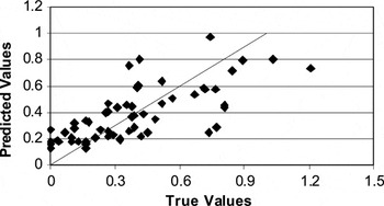
A plot of predicted values versus true values of the output is shown in Figure 1. Although most points have a deviation from the ideal line y = x and the smallest predicted value is 0.1, the points appear to be clustered around the ideal line and this model seems to capture the trends in the data.

Plot of predicted values versus true values of the average number of failures per day using the regression method.

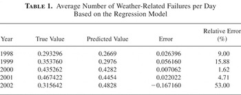
The model was also tested for its performance based on yearly aggregated data. The results of this analysis are shown in Table 1. These results appear to be quite good, except for 2002, which has a larger error.

Average Number of Weather-Related Failures per Day Based on the Regression Model

4. ONE-LAYER BAYESIAN NETWORK

A Bayesian network is a directed graphical model. Nodes represent random variables and arcs represent the relationship between the “starting” node and the “ending” node. For discrete Bayesian networks, every ending node is given a conditional probability table (CPT), known as the parameters of Bayesian networks [5,6]. The basic idea in the Bayesian network is to use a probabilistic approach to solve uncertainty problems in the real world. It has the powerful capacity to learn the orders from a large amount of seemingly scattered and intractable data. After learning from data, which means obtaining both structure and parameters, the Bayesian network can be utilized to predict outputs or make decisions by probabilities propagation.

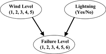
A simple one-layer Bayesian network with three nodes, representing the three random variables, as shown in Figure 2, is used to model the problem of this article. It is not only easily implemented but also has clearly explainable parameters, reflecting the residing statistical character in the occurrence of failures.

The Bayesian network for modeling failures on overhead feeders.

Wind gust is divided into five discrete levels, which are the same as those used in the previous model. Lightning is represented by a two-state random variable:

Failures are represented by a six-state random variable:

4.1. Conditional Probability Table

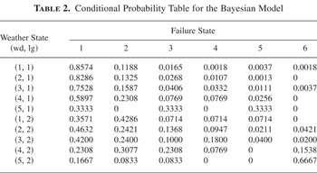
Only one conditional probability table is needed in this case, which is defined as P(Failure|Lightening, Wind). With the known structure and fully observed data, the maximum likelihood estimates of the parameters of CPT can be found [2]. A Bayes Net Toolbox Matlab package [3] was used to learn the parameters from data, which are shown in Table 2.

Conditional Probability Table for the Bayesian Model

Results in Table 2 represent the relationship between different lightning–wind states and failure states in a probabilistic way. Five states of wind and 2 states of lightning make up 10 circumstances. Given any of the 10 circumstances, the distribution of failures can be directly seen from Table 2.

4.2. Model Performance

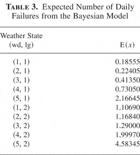
Since every circumstance can lead to any of the failure states, the expected number of failures in every circumstance is of interest and can be calculated using

where wd_i is wind state i (i = 1, 2, 3, 4, or 5), lg_j is lightning state j (j = 1 or 2), 4.5 is the average number of failures in failure state 5, 6.5 is the average number of failures in failure state 6, E(fl) is the expected number of failures, and P(fl_k|wd_i,lg_j) is the conditional probability from Table 2.

Results are shown in Table 3. The increasing trend in the expected number of failures with increasing wind levels is apparent in each lightning state. Also, the expected number of failures in lightning days is clearly above the ones in nonlightning days. These trends are consistent with the common experience.

Expected Number of Daily Failures from the Bayesian Model

As mentioned previously, variables lg and w1–w5 can be regarded as the probabilities of their corresponding events. Then the joint probabilities of lightning and each wind level can be obtained in the same way. Data were aggregated on a monthly basis. The law of total probabilities gives

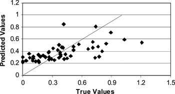
Once the probabilities of failures in each state were obtained, (4) was used again to get the expected number of failures for every month. A plot of true values versus predicted values of the average number of failures per day with an rsme value of 0.22084 calculated using (3) is shown in Figure 3. Points are clustered around the ideal line y = x, although deviation exists. The trend in this plot is quite similar to the plot in the regression method.

Plot of predicted values versus true values of the average number of failures per day using the Bayesian method.

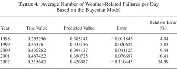
The results based on data aggregated on a yearly basis are shown in Table 4. The error terms from 1998 to 2001 are quite small, but 2002 renders the worst result, when the relative error increased to 35%. A comparison with the regression model shows that regression did better in 2000 and 2001, whereas the Bayesian network model did better in 1998 and 1999. However, both models had large errors in 2002.

Average Number of Weather-Related Failures per Day Based on the Bayesian Model

In order to track the origin of large errors, yearly aggregated data from 1998 to 2002 were examined and it was found that 2002 had worse weather but fewer failures than the other 4 years. This implied that both models actually predicted more failures based on worse weather in 2002 than the other 4 years. The failure records of 2002 need further scrutiny.

5. CONCLUSION

Two methods are presented in this article for predicting weather-related failures for Manhattan, Kansas. There are two limitations of the model. First, it was assumed that the effect of trees had not varied substantially from 1998 to 2002 and the feeders' condition had not eroded much for these 5 years. In other words, only if the effects of these factors were constant would the model have accurately predicted weather-related failures. Second, randomness exists in the occurrence of failures. Even with all of the factors having the same value, the number of failures for each day or each feeder would not have the same number most of the time.

A solution to the first problem is to include the other factors in the model. A solution to the second problem is to use enough data to overtake randomness. As can be seen in both models, better predictions were obtained with yearly aggregated data, whereas comparably large errors were produced on monthly aggregated data.

The two methods of this article have comparable performance. In fact, the input variables used in the regression method could be explained as the probabilities of the corresponding events. Consequently, the first method could be regarded as a way to regress on probabilities, whereas the Bayesian network method is a probabilistic approach. Thus, both methods have an association to probabilities. However, the Bayesian network method is preferred over the regression method since the meaning of the Bayesian network's parameters is straightforward and explainable. Moreover, the Bayesian network will be easier to expand when more variables are included.

Acknowledgment

The authors thank Westar Energy, Topeka, Kansas for providing the data for this work.

References

REFERENCES

Gupta, S., Pahwa, A., Brown, R.E., & Das, S. (2002). A fuzzy model for overhead distribution feeders failure rates. In Proceedings of the 34th North American Power Symposium.

Heckerman, D. (1998). A tutorial on learning with Bayesian networks. In M. Jordan (ed.), Learning in graphical models. Cambridge, MA: MIT Press.

Murphy, K. (2001). The Bayes Net Toolbox for Matlab. Computing Science and Statistics 33: 331–350.Google Scholar

Neter, J., Kutner, M., Wasserman, W., & Nachtsheim, C. (1996). Applied linear statistical models, 4th ed. New York: McGraw Hill.

Pearl, J. (1988). Probabilistic reasoning in intelligent systems: Networks of plausible inference. San Mateo, CA: Morgan Kaufmann.

Pearl, J. (2002). Causality: Models, reasoning and inference. Cambridge: Cambridge University Press.

Williams, C.W. (2003). Weather normalization of power system reliability indices. In Proceedings of IEEE PES T&D Conference and Expo.

Zhou, Y., Pahwa, A., & Das, S. (2003). A fuzzy Bayesian model for overhead distribution feeders failure rates. In Proceedings of the 35th North American Power Symposium.