

1. Introduction
Economic historians, using height as an indicator of the biological standard of living, have discovered several historical anomalies including the Antebellum Puzzle: a pattern of declining stature among American men despite a growing economy in the years before the Civil War (Komlos Reference Komlos1987; Fogel Reference Fogel1994; Steckel Reference Steckel1995). Much work has been done to understand the causes of this decline in the biological standard of living prior to the Civil War. Studies of postbellum stature, on the other hand, were either regionally limited or used peculiar populations such as Steckel and Haurin's (Reference Steckel, Haurin and Komlos1994) Ohio National Guardsmen, Komlos and Coclanis’ (Reference Komlos, Coclanis and 1995) Citadel students, Sunder's (Reference Sunder2007) passport applicants, Maloney and Carson's (Reference Maloney, Carson and 2008) and Carson's (Reference Carson2009) prison inmates, and Hiermeyer's (Reference Hiermeyer2008) continuation of Komlos’ (Reference Komlos1987) analysis of West Point cadets. This, however, is the first large nationwide study to analyze the stature of the common man in the postbellum period.
The period from 1850 to 1890 is of great interest not only because of the Civil War but also because it was a time of rapid growth in GDP, industrial production, urbanization, transportation and communication, all of which dramatically changed the US economy. The analysis of physical stature enables us to assess the impact of these developments on the standard of living of the US population, since these data supplement the evidence derived from conventional measures. These conventional measures show substantial gains in GDP (87%) and GNP (74%) per capita and industrial productionFootnote 1 (600%) during the period under consideration despite the Civil War (Rhode Reference Rhode2002; Davis Reference Davis2004; Sutch Reference Sutch, Carter, Gartner, Haines, Olmstead, Sutch and Wright2006).
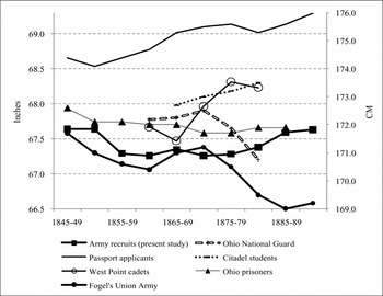
In the current estimates heights increase in 1880 rather than decrease as in Fogel's extrapolation from the Ohio National Guard, which has become conventional wisdom. This new evidence presents a different picture, one based on more solid evidence. Our findings are more optimistic than those that had become commonly accepted, insofar as they imply that heights began to recover earlier than commonly asserted. Although the estimates reported in this article, based on a nationwide sample, correspond to the extrapolation quite well until about the 1870s, thereafter they diverge substantially. The difference by 1890 is 1.02 in. (2.6 cm). Thus, by correcting Fogel's (Reference Fogel1986) estimate, the present study bridges a gap in human-height analysis, shedding light on one of the darkest eras in terms of this measurement of biological wellbeing in US history.
2. Data and methodology
We sampled 58,512 US Army recruitsFootnote 2 who enlisted between 1898 and 1912. The data set, with recruits born between 1847 and 1894, includes each recruit's name, date of enlistment, place of enlistment, duration of his service, place of birth, occupation, height, regiment and the number of times he enlisted.Footnote 3
The recruits were assigned state and county National Historical Geographic Information System (NHGIS) codes that identified their counties of birth. This geo-coding process allowed us to combine the enlistment records with county-level statistics from the 1880 US Census (Minnesota Population Center 2004).
We find that there was a minimum height requirement (MHR) of 64 in. (162.6 cm) to join the military, therefore truncated maximum likelihood estimation (TMLE) is used for consistent estimates (Komlos Reference Komlos2004).Footnote 4 Some models are estimated with a constrained standard deviation of today's adult population, which is 2.7 in. (6.86 cm), according to Frisancho (Reference Frisancho1990) and Cole (Reference Cole2000). The advantage of restricting the standard deviation of height is increased precision and reduced variance, but it might bring about a trade-off between bias and precision of the estimator. That is why we present estimation both ways, with and without constraining the standard deviation of the height distribution. Simulations show that the restriction's effect on time trends in heights and explanatory variables is minimal but the effect on levels can be substantial (A'Hearn Reference A'Hearn2004).
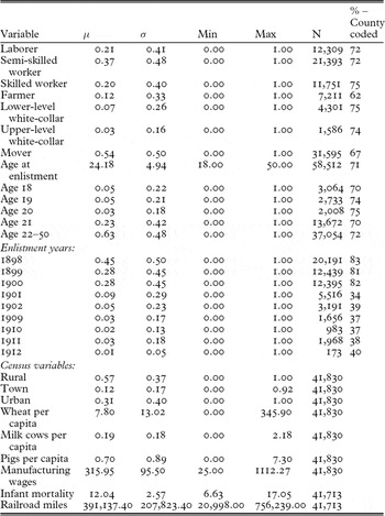
Descriptive statistics

Notes: Laborer includes those with unknown occupations. A mover enlisted in a state other than his state of birth and a stayer enlisted in his state of birth. Wheat per capita is measured in 100 bushels. Manufacturing wages are annual manufacturing wages per manufacturing worker. Infant mortality is measured in infant deaths per 1,000 births. Railroad miles are miles in a state completed as of June 1st 1880.% – County is the percentage of the full sample that could be county-coded.
Sources: See the text.
First, we estimate time trends for height in the sample with controls for standard census regions and divisions of birth. Thereafter we include county-level variables in order to test how urbanization, the availability of nutrients, wages, transportation, geographic mobility and the epidemiological framework affected stature, as in Craig and Weiss (Reference Craig, Weiss, Komlos and Baten1998), Haines, Craig and Weiss (Reference Haines, Craig and Weiss2003) and Sunder (Reference Sunder2007).
At the county-level, we begin by examining the hypothesis that population density affected height. During the period of US history under consideration, poor sanitation and overcrowded living conditions in urban areas facilitated the transmission of diseases. These, in turn, stunted growth (Preston and Haines Reference Preston, Haines and 1991; Steckel Reference Steckel1995; Lee Reference Lee1997). In order to distinguish varying degrees of urbanization, three census categories are adopted.Footnote 5 The reference category is rural, that is, agglomerations of no more than 2,500 inhabitants. The other categories are towns with populations between 2,500 and 25,000 and urban areas with more than 25,000 inhabitants. Another proxy variable that captures the disease environment at the state level is the infant mortality rate.Footnote 6 The effect of infant mortality on heights is expected to be negative because the diseases that increase the infant mortality rate also consume energy that could otherwise be used for growth.
The agricultural-output variables (milk cows, pigs and wheat) reflect the local availability of nutrients. For instance, those living in counties with dairy and livestock operations faced lower prices for these products insofar as they did not have to pay transportation costs or for the profits of middlemen compared with urban dwellers, and as a consequence they would consume more calcium and protein. Thereby they would grow taller than those in locations with poorer access to these nutrients. One can thus infer that there should be a height premium for nutrient propinquity. Indeed, many studies have documented such a premium (Komlos Reference Komlos1987; Craig and Weiss Reference Craig, Weiss, Komlos and Baten1998; Haines, Craig and Weiss Reference Haines, Craig and Weiss2003). Moreover, in urban areas food was less nutritious because of losses during transportation (refrigeration was just beginning) (Komlos Reference Komlos1987; Craig, Goodwin and Grennes Reference Craig, Goodwin and Grennes2004). In particular, dairy products, rich in protein and calcium, could not be transported over long distances without spoilage, so milk cows per capita should influence height locallyFootnote 7 (Baten Reference Baten1999). Beginning in the 1870s, improvements in transportation and refrigeration meant that dairy products could be shipped over longer distances than before (Bateman Reference Bateman1968). The meat industry, too, was transformed by these improvements. Dressed beef, for example, could be transported, whereas previously, livestock had to be transported close to the market in question and only then slaughtered and dressed (Yeager Reference Yeager1970). Hence, market integration, made possible by improvements in transportation, influenced nutritional status positively by price and quality in urban areas and negatively by price alone in rural surplus food areas. For urban dwellers, market integration could lead to a better and more balanced diet promoting growth because healthy food would become more available and affordable, while for (rural) nutrient-exporting regions, it could lead to a substitution away from protein- and calcium-rich foods to a carbohydrate-based diet, because farm-gate prices for protein-rich foods were very high (Komlos Reference Komlos1987, Reference Komlos1996; Craig and Weiss Reference Craig, Weiss, Komlos and Baten1998). Transportation, however, promotes access not only to markets but also to diseases, so its net effect on height is ambiguous. The diseases that could be spread through transportation networks would most likely affect primarily rural dwellers, who were not previously exposed to these diseases because they were living in sparsely populated areas with healthier environments (Haines Reference Haines2004). Our proxy variable for market integration is the length of railroad lines completed in each state as of 30 June 1880 (measured in 1,000 miles).
We use the nominal annual manufacturing wage per worker as a proxy for (non-farm) incomes. Higher income was accompanied by higher meat consumption, and animal protein promotes growth (Cuff Reference Cuff2005). Furthermore, a rise in income permits a move to better housing, which is associated with a decline in illness and in infant mortality (Preston and Haines Reference Preston, Haines and 1991). We also include categories for the recruits’ civilian occupations before enlistment to control for the socioeconomic background.Footnote 8 These occupations were coded into the following categories: farmers, laborers (including those temporarily unemployed or with no reported occupation), semi-skilled blue-collar workers, skilled blue-collar workers, lower-level white-collar workers and upper-level white-collar workers. Recruits from higher socioeconomic strata are expected to be taller than the others, in line with findings by Komlos (Reference Komlos1987), Steckel (Reference Steckel1995), Sunder (Reference Sunder2007) and Hiermeyer (Reference Hiermeyer2008). On the other hand, it is possible that those who were taller and healthier than average were also more productive and therefore had better-paying jobs in adulthood, so the direction of the causality is not clear (Lee Reference Lee1997).
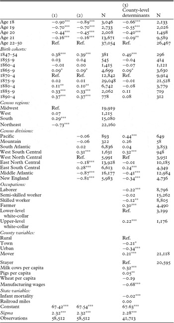
Height of US Army recruits nationwide: truncated normal regression (in inches)

Notes: * p < 0.10, ** p < 0.05, *** p < 0.01. Sigma denotes the estimated standard deviation of heights. ‘Laborer’ includes those with unknown occupations. ‘Rural’ is the proportion of county inhabitants living in places with fewer than 2,500, ‘Town’ with more than 2,500 and fewer than 25,000, and ‘Urban’ with more than 25,000 inhabitants. A mover enlisted in a state other than his state of birth and a stayer enlisted in his state of birth. Wheat is measured in 100 bushels. Manufacturing wages are annual manufacturing wages per manufacturing worker in $1,000. Infant mortality is measured in infant deaths per 1,000 births. Railroad miles are miles in a state completed as of 1 June 1880 in 10,000 miles.
Sources: See the text.
A recruit who enlisted out of state is classified as a mover. There are two hypotheses regarding movers: that they were mostly poorFootnote 9 and malnourished (and therefore shorter than average) and so moved to another state in the hope of improving their lot; or that moving was costly and therefore movers were also well nourished (and taller than average) (Craig and Weiss Reference Craig, Weiss, Komlos and Baten1998; Haines, Craig and Weiss Reference Haines, Craig and Weiss2003).
3. Results
3.1. Time trends in height
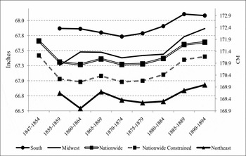
Heights declined in the 1850s, then leveled off and stagnated until they increased in the 1880s. This trend is unchanged when the sample is restricted to adults only, and there is a height gradient rising from the Northeast towards the South and the West. Nationwide trends show a decline in heights after 1854, stagnation until 1879 followed by increasing heights thereafter.Footnote 10 The trends over time differed by region: the South was the tallest region and experienced stagnation until 1880, the Midwest was second with stagnation until 1885, and the Northeast trailed, with declines in the 1850s followed by stagnation (Figure 1). The height prediction from the constrained estimation is consistently lower by about 0.3 in. (0.8 cm) although the trends are identical.
Nationwide and regional estimated height of US-born adult recruits
Notes: Estimated heights are weighted with the proportion of white adult males in each region or state. Constrained estimates are estimated with the standard deviation set to 2.7 in. (6.86 cm). Regional height regressions are available from the author upon request. Sources: Table 2.

On average Southern recruits were the tallest (67.69 in.; 171.9 cm) followed by the West (67.46 in.; 171.3 cm) and Midwest (67.40 in.; 171.2 cm), while Northeasterners (66.67 in.; 169.3 cm) were the shortest. The results by smaller census divisionsFootnote 11 are similar: recruits from the West South Central division were the tallest (67.85 in.; 172.3 cm), followed by East South Central (67.82 in.; 172.3 cm), the South Atlantic (67.56 in.; 171.6 cm), West North Central (67.54 in.; 171.6 cm), Pacific and Mountain (67.48 in.; 171.4 cm) and East North Central (67.36 in.; 171.1 cm). The two shortest divisions were New England (66.73 in.; 169.5 cm) and Middle Atlantic (66.67 in.; 169.3 cm). The difference between the shortest and tallest region was 1.02 in. (2.6 cm) and 1.18 in. (3 cm) among divisions. Recruits from the South and in particular from the East South Central and the West South Central divisions remained the tallest, despite the Civil War.Footnote 12 Southerners could retain their status as the tallest Americans insofar as the relatively low urbanization and population density meant that their disease load was less than that in other parts of the country. Moreover, the emancipation of slaves affected primarily the output of non-edibles. It is nonetheless amazing that agricultural productivity was retained sufficiently to maintain the nutritional status of children and youth as reflected in their height. This is remarkable, because after the Civil War self-sufficiency was decreasing, the number of hogs and corn per capita was declining, and the cotton to corn ratio doubled between 1850 and 1890 (Wright and Kunreuther Reference Wright and Kunreuther1975).
3.2. Long-run perspectives
Figure 2 compares our findings with those of other studies of this time period including with Fogel's (Reference Fogel1986) estimate, which is partly extrapolated from the Ohio National Guard data. These latter data have been reproduced so often that they have become a standard in the literature without noting that they are based on extrapolation (e.g. Historical Statistics of the United States (Steckel Reference Steckel, Carter, Gartner, Haines, Olmstead, Sutch and Wright2006)). We show that Fogel's estimates, which have become conventional wisdom, are flawed. While Fogel finds a decline in heights that begins in the early 1870s and bottoms out in the late 1880s, this study shows that the nationwide trend followed a very different pattern. We find that height was not declining but still stagnating in the 1870s and started to increase in the early 1880s. In the most extreme case, Fogel underestimates true adult heights by as much as 1.02 in. (2.6 cm) in 1890. Other studies of height in this time period use smaller samples or peculiar populations. West Point cadets and Citadel students were for the most part children of upper-middle-class parents, which explains their above average stature (Komlos Reference Komlos1987; Komlos and Coclanis Reference Komlos, Coclanis and 1995; Hiermeyer Reference Hiermeyer2008). Passport applicants were much taller than Army recruits and their heights continuously increased in the period under consideration. This height premium is due to the fact that the median passport household's socioeconomic status was in the 95th percentile of all white households because in the nineteenth century travel was prohibitively expensive for all but the wealthy (Sunder Reference Sunder2007). Maloney and Carson's (Reference Maloney, Carson and 2008) study finds a similar trend over time, but their data are limited to those who had been convicted of a crime and were incarcerated in Ohio.
Comparison with other studies
Sources: Fogel's Union Army (Fogel Reference Fogel1986, Reference Fogel2004), West Point cadets (Komlos Reference Komlos1987), Ohio National Guard (Steckel and Haurin Reference Steckel, Haurin and Komlos1994), Citadel students (Komlos and Coclanis Reference Komlos, Coclanis and 1995), passport applicants (Sunder Reference Sunder2007), white Ohio prisoners (Maloney and Carson Reference Maloney, Carson and 2008), Army recruits (see the text).

3.3. County-level determinants of height
County-level determinants of height are analyzed for all those that could be assigned to their county of birth. The proportion of a given county population living in towns with more than 2,500 inhabitants had a negative effect on adult height. The proportion of people living in urban areas with more than 25,000 people also had a significant and negative effect on stature – of almost twice the magnitude of the town category. In other words, a high population density brought about by urbanization had a negative effect on adult height.Footnote 13 The state infant-mortality rates had a significant and negative effect on stature, confirming the hypothesis that it was the above-average disease rate in an unhealthy environment that contributed to an above-average infant-mortality rate and also led to below-average adult heights.
Milk cows and pigs per capita had a significant and positive effect on height confirming the propinquity thesis, whereas wheat per capita had no significant effect.Footnote 14 Although grain provides energy in the form of carbohydrates, compared to meat and dairy products it contains much less calcium and protein, which are essential for growth (especially animal protein) (Waterlow Reference Waterlow1994). There was no significant correlation between the number of miles of state rail lines and average height. A valid explanation could be technical: that the high level of aggregation fails to capture the county-by-county variation in railroad access.
Upper-level white-collar workers enjoyed a significant height premium, of 0.22 in. (0.6 cm), compared with lower-level white-collar workers, but laborers experienced a significant height penalty of 0.22 in. (0.6 cm). Surprisingly, skilled workers also experienced a height penalty of 0.12 in. (0.3 cm). Only the height of semi-skilled workers was not significantly different from that of lower-level white-collar workers. The premium for farmers of about 0.30 in. (0.8 cm) also supports the propinquity hypothesis.Footnote 15
Our proxy for income, the nominal manufacturing wage per capita, had a significant and negative effect on stature. This variable probably picks up the costs of living because income is nominal and therefore positively correlated with costs of living in a county. It is also most likely capturing the effects of the degree of industrialization. Our data on those who move out of state support the second hypothesis that movers were taller, and are in line with the finding of Haines, Craig and Weiss (Reference Haines, Craig and Weiss2003) that movers were on average 0.2 in. (0.5 cm) taller than those who remained in the state where they had been born.
4. Conclusion
This study of the physical stature of US-born soldiers born c. 1850–90 fills a lacuna in the literature. Previous anthropometric studies on this period tend to be either regionally limited or are limited to the elite segment of the population. This is the first study of a national data set based on a large sample of US Army recruits. In addition to estimating the trend in heights for the whole nation in this period, the study also examines how and to what degree local nutrient production, urbanization, market integration, occupations and the disease environment affected stature.
The most noteworthy result that emerges from this evidence is that average heights in the US began rising much earlier than has previously been thought compared with the extrapolated trend derived from Ohio. We find that the decline in physical stature that had begun in the 1830s, as found in previous studies, continued into the 1850s. The decline in the 1850s was about 0.4 in. (1 cm) from 67.64 in. (171.8 cm) in the early 1850s birth cohort to a nadir of 67.26 in. (170.8 cm) in the cohort born during the Civil War, and heights remained virtually unchanged until the 1880s, when they started to recover. Average regional heights ranged from a high of 67.69 in. (171.9 cm) in the South to a low of 66.67 in. (169.3 cm) in the Northeast. Despite the Civil War, the South consistently had the tallest residents, with no significant changes in stature between the early 1850s and the late 1870s, while the Northeastern residents had the shortest stature just as before the war.
Moreover, we find that protein and calcium availability had a significant and positive effect on height similar to findings by Craig and Weiss (Reference Craig, Weiss, Komlos and Baten1998) and Haines, Craig and Weiss (Reference Haines, Craig and Weiss2003). Urbanization had a significant and negative effect on height, as did infant mortality, which was used as an indicator for the disease environment. As for height differences according to occupation, the tallest were upper-level white-collar workers, who could afford better than average food and housing, and farmers, who enjoyed lower relative prices and greater than average proximity to food sources (Komlos Reference Komlos1987; Lee Reference Lee1997)
While this study confirms, in the main, the conclusions of previous studies concerning the correlates of height, it also reveals considerable regional variability. The rapid economic growth that accompanied urbanization, industrialization and market integration brought nineteenth-century Americans many benefits, but they came at a price: the diminution in height in the antebellum period was followed by an extended period of stagnation during reconstruction, which implies that the biological wellbeing of the population failed to improve in spite of the prosperity of the period. This should caution against automatically equating GNP estimates with welfare. Not until the birth cohorts of the 1890s did the benefits of economic growth affect the biological standard of living of the common people. In contrast, the height of the elite, both men and women, had been increasing rapidly beginning with the 1850s. Hence, quite a considerable gulf developed between the average and the elite segments of the society: in 1850 passport applicants were 0.91 in. (2.3 cm) taller than Army recruits; however, by 1890 the gap had almost doubled to 1.65 in. (4.2 cm). Yet by 1890 the common man had reached the 1850 level again after decades of stagnation. The benefits of economic growth were beginning to filter down to the masses.
Acknowledgements
I am grateful for the advice and support of John Komlos. I thank Takeshi Amemiya, Francesco Cinnirella, Michael Haines, Daniel Koch, Linda Rousova, Michael Specht, Susan Stewart, Marco Sunder, Marianne Wanamaker, Thomas Weiss and Gordon Winder for helpful comments and conversations. I thank two anonymous referees for helpful comments. I am also grateful to the seminar participants at the Economic History Association's 2009 meeting for valuable comments and suggestions.