1 Introduction
1.1 Motivation
In recent years, relational data have grown at a tremendous rate; it is present in domains such as the Internet and the World Wide Web (Albert et al., Reference Al Hasan and Zaki1999; Faloutsos et al., Reference Faloutsos, Faloutsos and Faloutsos1999; Broder et al., Reference Broder, Kumar, Maghoul, Raghavan, Rajagopalan, Stata, Tomkins and Wiener2000), scientific citation and collaboration (Newman, Reference Newman2001; McGovern et al., Reference McGovern, Collier, Matthew Gagne, Brown and Rodger2003), epidemiology (Kleczkowski & Grenfell, Reference Kleczkowski and Grenfell1999; Moore & Newman, Reference Moore and Newman2000; May & Lloyd, Reference May and Lloyd2001; Pastor-Satorras & Vespignani, Reference Pastor-Satorras and Vespignani2001), communication analysis (Rossi & Neville, Reference Rossi and Gleich2010), metabolism (Jeong et al., Reference Jeong, Mason, Barabasi and Oltvai2000; Wagner & Fell, Reference Wagner and Fell2001), ecosystems (Camacho et al., Reference Camacho, Guimerà and Nunes Amaral2002; Dunne et al., Reference Dunne, Williams and Martinez2002), bioinformatics (Jeong et al., Reference Jeong, Tombor, Albert, Oltvai and Barabási2001; Maslov & Sneppen, Reference Maslov and Sneppen2002), fraud and terrorist analysis (Krebs, Reference Krebs2002; Neville et al., Reference Neville, Simsek, Jensen, Komoroske, Palmer and Goldberg2005), and many others. The links in these data may represent citations, friendships, associations, metabolic functions, communications, co-locations, shared mechanisms, or many other explicit or implicit relationships.
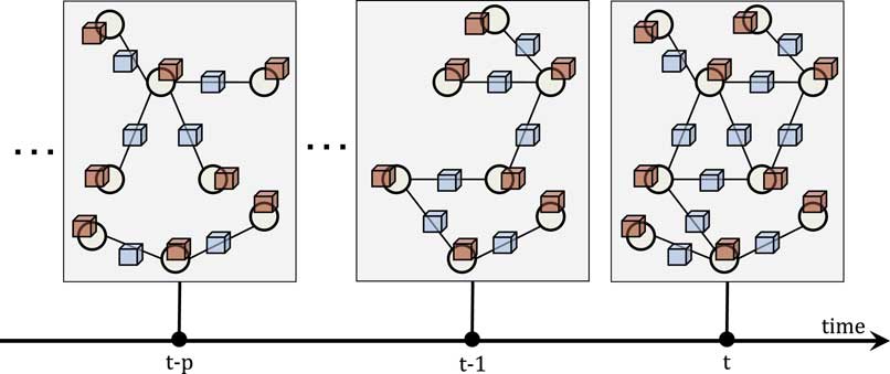
The majority of these real-world relational networks are naturally dynamic—evolving over time with the addition, deletion, and changing of nodes, links, and attributes. Despite the fundamental importance of these dynamics, the majority of work in relational learning has ignored the dynamics in relational data (i.e. attributed network data). In particular, dynamic attributed graphs have three main components that vary in time. First, the attribute values (on nodes or links) may change over time (e.g. research area of an author). Next, links might be created and deleted throughout time (e.g. host connections are opened and closed). Finally, nodes might appear and disappear over time (e.g. through activity in an online social network). Figure 1 provides an intuitive view of these underlying dynamics.
Relational time series data

Previous research in machine learning (ML) assumes independently and identically distributed data (IID) (Anderson et al., Reference Anderson, Michalski, Michalski, Carbonell and Mitchell1986; Bishop et al., Reference Bishop2006); and has ignored relational dependencies (and temporal dependencies). This independence assumption is often violated in relational data as (relational) dependencies among data instances are naturally encoded. More specifically, relational autocorrelation is a correlation or statistical dependence between the values of the same attribute across linked instances (Jensen et al., Reference Jensen, Neville and Gallagher2004) and is a fundamental property of many relational data sets. For instance, people are often linked by business associations, and information about one person can be highly informative for a prediction task involving an associate of that person. Recently, statistical relational learning (SRL) methods (Getoor & Taskar, Reference Getoor and Taskar2007) were developed to leverage the relational dependencies (i.e. relational autocorrelation (Rossi et al., Reference Rossi, Gleich, Gebremedhin and Patwary2012b), also known as homophily (McPherson et al., Reference McPherson, Smith-Lovin and Cook2001); between nodes (Friedman et al., Reference Friedman, Getoor, Koller and Pfeffer1999; Macskassy & Provost, Reference Macskassy and Provost2003; Neville et al., Reference Neville, Jensen and Gallagher2003; De Raedt & Kersting, Reference Deng and Li2008; McDowell et al., Reference McDowell, Gupta and Aha2010). In many cases, these relational learning methods improve predictive performance over traditional IID techniques (Macskassy & Provost, Reference Macskassy and Provost2003; Neville et al., Reference Neville, Jensen and Gallagher2003; McDowell et al., Reference McDowell, Gupta and Aha2009).
Relational learning methods have been shown to improve over traditional ML by modeling relational dependencies, yet they have ignored temporal information (i.e. explicitly assumes the data are independent with respect to time). In that same spirit, our work seeks to make further improvements in predictive performance by incorporating temporal information and designing methods to accurately learn, represent, and model temporal and relational dependencies. The temporal information is known to be significantly important to accurately model, predict, and understand relational data (Watts & Strogatz, Reference Watts and Strogatz1998; Newman et al., Reference Newman, Barabasi and Watts2006). In fact, time plays a key role in many natural laws and is at the heart of our understanding of the universe, that is, the unification of space and time in physics (Einstein, Reference Einstein1906) and how time is related to space and vice versa is fundamentally important to our understanding and interpretation of the universe and its laws (Einstein, Reference Einstein1906; Bock et al., Reference Bock, Cooray, Hanany, Keating, Lee, Matsumura, Milligan, Ponthieu, Renbarger and Tran2008). We make a similar argument here, that ignoring time in attributed networks can only add further uncertainty, as time places a natural ordering on the network components, including the changing of attribute values, links, and nodes.
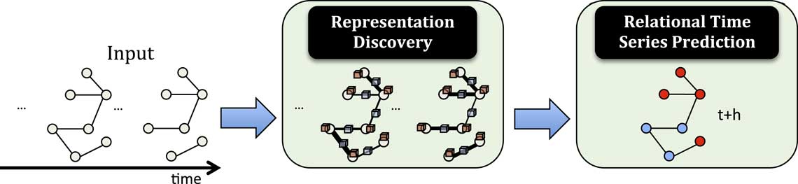
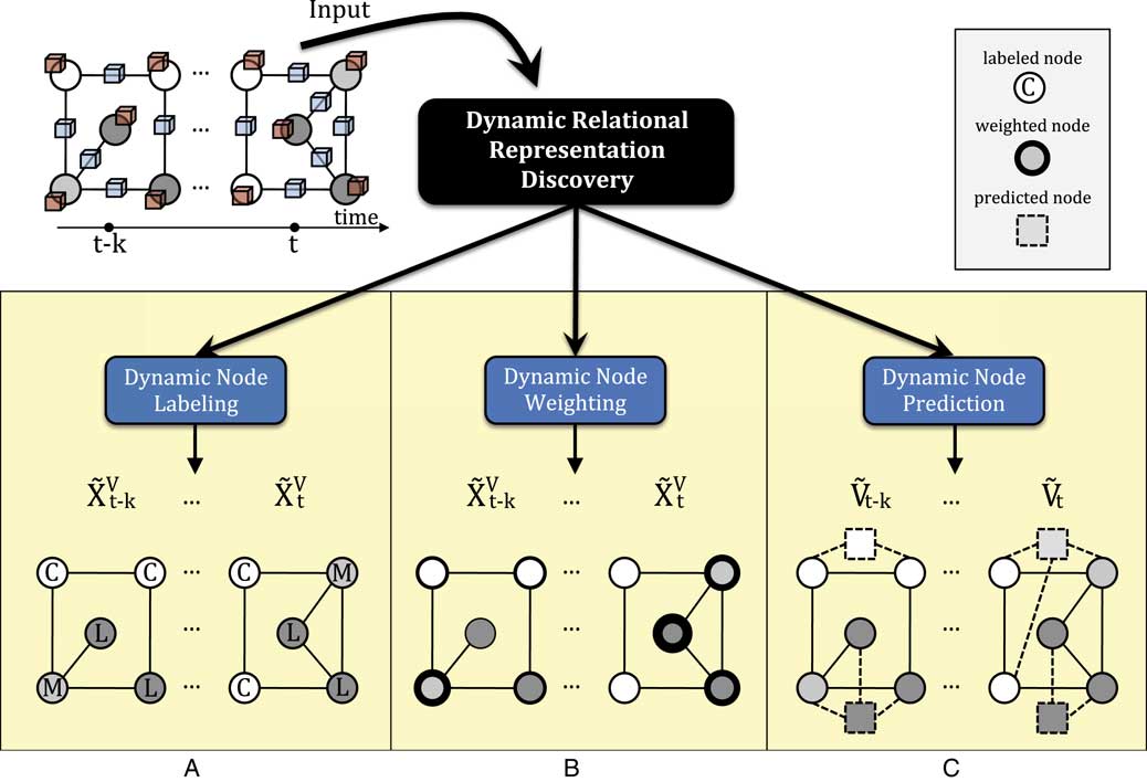
This work formulates the problem of relational time series learning and proposes a framework that consists of two main components as shown in Figure 2. The first component learns a feature-based representation from a collection of dynamic relational data ( i.e., a time series of graphs and attributes) given as input which incorporates the fundamental temporal dependencies in relational graph data. While the second component leverages the learned feature-based representation for relational time series prediction, which includes both relational time series classification models and regression. In other words, this work proposes techniques for learning an appropriate representation from dynamic attributed graph data for the purpose of improving accuracy of a given relational learningFootnote 1 (Getoor & Taskar, Reference Getoor and Taskar2007) task such as classification (Rossi et al., Reference Rossi, Gleich, Gebremedhin and Patwary2012b). We propose a taxonomy shown in Figure 4 for the fundamental representation tasks for nodes in dynamic attributed networks. This work focuses on the three fundamental representation tasks for dynamic attributed networks including dynamic node labeling, dynamic node weighting, and dynamic node prediction. As an aside, let us note that we do not focus on the (symmetric) link-based representation tasks since they have received considerable attention recently (in various other forms) (Hasan et al., Reference Hasan, Chaoji, Salem and Zaki2006; Liben-Nowell & Kleinberg, Reference Liben-Nowell and Kleinberg2007; Lassez et al., Reference Lassez, Rossi and Jeev2008; Acar et al., Reference Acar, Dunlavy and Kolda2009; Koren et al., Reference Koren, Bell and Volinsky2009; Xiang et al., Reference Xiang, Yuan, Zhao, Chen, Zhang, Yang and Sun2010a; Al Hasan & Zaki, Reference Albert, Jeong and Barabási2011; Menon & Elkan, Reference Menon and Elkan2011; Oyama et al., Reference Oyama, Hayashi and Kashima2011; Schall, Reference Schall2014) and therefore this work focuses on the novel dynamic representation tasks for nodes.
Overview of relational time series learning

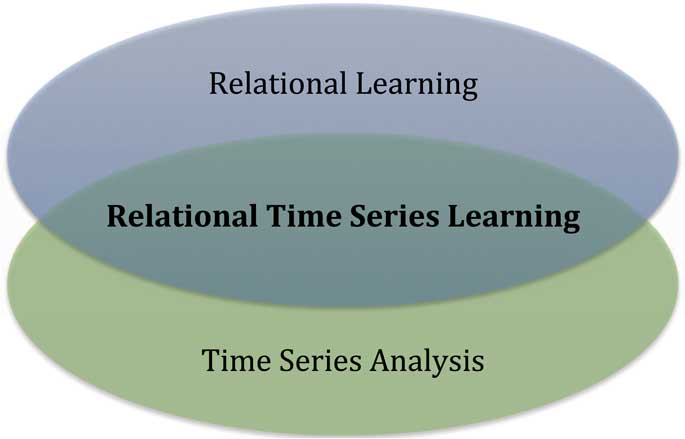
Ultimately, the goal of this work is to help further bridge the gap between relational learning (Friedman et al., Reference Friedman, Getoor, Koller and Pfeffer1999; Macskassy & Provost, Reference Macskassy and Provost2003; Neville et al., Reference Neville, Jensen and Gallagher2003; Getoor & Taskar, Reference Getoor and Taskar2007; De Raedt & Kersting, Reference Deng and Li2008; McDowell et al., Reference McDowell, Gupta and Aha2010; Rossi et al., Reference Rossi, Gleich, Gebremedhin and Patwary2012b) and traditional time series analysis (Pindyck & Rubinfeld, Reference Pindyck and Rubinfeld1981; Clements & Hendry, Reference Clements and Hendry1998; Croushore & Stark, Reference Croushore and Stark2001; Brockwell & Davis, Reference Brockwell and Davis2002; Marcellino et al., Reference Marcellino, Stock and Watson2006; Ahmed et al., Reference Ahmed, Atiya, El Gayar and El-Shishiny2010; Box et al., Reference Box, Jenkins and Reinsel2013) (see Figure 3). This gap between these fundamentally important problems seemingly arose due to the fact that the majority of relational learning techniques from the ML community has ignored temporal or dynamic relational data (Chakrabarti et al., Reference Chakrabarti, Dom and Indyk1998; Friedman et al., Reference Friedman, Getoor, Koller and Pfeffer1999; Domingos & Richardson, Reference Domingos and Richardson2001; Macskassy & Provost, Reference Macskassy and Provost2003; Neville et al., Reference Neville, Jensen and Gallagher2003; Getoor & Taskar, Reference Getoor and Taskar2007; De Raedt & Kersting, Reference Deng and Li2008; McDowell et al., Reference McDowell, Gupta and Aha2010), whereas the time series work has ignored graph data and has mainly focused on (i) modeling independent time series or (ii) multiple time series that are assumed to be completely correlated (Pindyck & Rubinfeld, Reference Pindyck and Rubinfeld1981; Brockwell & Davis, Reference Brockwell and Davis2002; Ahmed et al., Reference Ahmed, Atiya, El Gayar and El-Shishiny2010; Box et al., Reference Box, Jenkins and Reinsel2013). The intersection of these two areas is relational time series learning and differs significantly from relational learning and time series analysis in the data utilized, model and data assumptions, and their objectives. For instance, the prediction objective of the relational learning problem is mainly for within-network or across-network prediction tasks and does not predict the future node attribute values. Relational learning does not utilize or model temporal information, whereas time series analysis lacks relational information. There are many other differences discussed later.
Toward bridging the gap between relational learning and time series analysis. The focus of this work is on the intersection between these two areas which we call Relational Time Series Learning. Relational learning has primarily focused on static relational graph data (graphs+attributes), whereas the time series analysis literature avoids graph data and instead focuses on independent time series (i.e. modeling each of time series disjointly) or time series that are assumed to be completely dependent (i.e. clique).

1.2 Scope of this article
This article focuses on the problem of relational time-series forecasting and techniques for learning dynamic relational representations from graph data with timestamps. We do not focus on dynamic network analysis and mining. However, whenever possible, we do reinterpret techniques that were proposed for different problems, and discuss how they could potentially be used for relational time series representation learning for improving relational time series forecasting. As an aside, the relational time series forecasting methods may also be useful for other applications (i.e. besides predicting node attributes) including dynamic network analysis (Tang et al., Reference Tang, Musolesi, Mascolo, Latora and Nicosia2010; Holme & Saramäki, Reference Holme and Saramäki2012), anomaly detection (Bunke & Kraetzl, Reference Bunke and Kraetzl2004; Chandola et al., Reference Chandola, Banerjee and Kumar2009) in dynamic graphs (Noble & Cook, Reference Noble and Cook2003; Ide & Kashima, Reference Ide and Kashima2004; Tong & Lin, Reference Tong and Lin2011; Rossi et al., Reference Rossi, McDowell, Aha and Neville2013a), dynamic ranking (O’Madadhain & Smyth, Reference O’Madadhain and Smyth2005; Das Sarma et al., Reference Das Sarma, Gollapudi and Panigrahy2008; Rossi & Gleich, Reference Rossi, Gallagher, Neville and Henderson2012), among many other ML tasks and applications (Rossi et al., 2013Reference Rossi and Nevilleb, Reference Rossi and Neville2013c; Rossi, Reference Rossi2014). However, this is outside the scope of this article.
1.3 Overview
This article is organized as follows: Section 2 introduces and defines the relational time series forecasting problem, which consists of relational time series classification (Section 2.1) and regression (Section 2.2). Next, Section 3 presents the relational time series representation learning for relational time series forecasting. Section 4 surveys and reinterprets existing work for use in the relational time series representation learning and forecasting problem. Section 5 presents a few important open and challenging problems. Finally, Section 6 concludes.
2 Relational time series forecasting
Using the learned representation, we demonstrate the effectiveness of these techniques for relational time series classification and regression of dynamic node attributes. We define relational time series classification (Section 2.1) and regression (Section 2.2) more precisely below.
2.1 Relational time series classification
Problem 1 (Relational Time Series Classification). Given a ‘known’ time series of attributed graph data
 ${\cal G}\,{\equals}\,\left\{ {{\bf G}_{1} ,...,{\bf G}_{t} } \right\}$
for learning, the task is to infer the class labels Y
t+h
of the nodes at time t+h in the graph where L refers to the set of possible labels.
As an aside, if h=1 then we call this one-step ahead prediction, whereas multi-step ahead prediction refers to the case when h>1, and thus the prediction is across multiple timesteps. Our relational time series classification methods are also flexible for both binary (i.e. |L|=2) and multi-class problems (i.e. |L|>2), whereas binary classification has been the primary focus of the past relational learning methods for static graphs. Similarly, we also investigate the relational time series regression problem.
2.2 Relational time series regression
Problem 2 (Relational Time Series Regression). Given a time series of attributed graphs
 $${\cal G}\,{\equals}\,\left\{ {{\bf G}_{1} ,...,{\bf G}_{t} } \right\}$$
, the task is to estimate the real-valued variable
 ${\bf{Y}} {\rm }_{{t{\plus}h}} \in{\Bbb R}^{n} $
at time t+h for the nodes in the graph.
The prediction task investigated in this paper is also fundamentally different than the traditional relational learning problems/assumptions. More specifically, we define within-network (e.g. inference) as the task where training instances from a single (static) graph are connected directly to instances whose classification labels are to be predicted (McDowell et al., Reference McDowell, Gupta and Aha2009; Xiang et al., Reference Xiang, Neville and Rogati2010b). Conversely, the task of across-network inference attempts to learn a model on a (static) network and applying the learned models to a separate network (Craven et al., Reference Craven, DiPasquo, Freitag, McCallum, Mitchell, Nigam and Slattery1998; Lu & Getoor, Reference Lu and Getoor2003). For instance, we may learn a model from a static and/or aggregated graph from Facebook and use that learned model for prediction on another social network such as Google+ or Twitter. While both prediction problems for relational learning assume a static network, they also differ fundamentally in their underlying assumptions and goals. On the other hand, we focus on using the past time series of attributed graphs where the training nodes may be connected directly to nodes whose classification labels are to be predicted and similarly the past time series observations of the prediction attribute may also be directly used. The fundamental idea is that both past relational and temporal dependencies and information may be used to predict the future time series values of a given attribute. We also note that we may learn a model using some past data and use it to predict the future value at t+h of an attribute time series, or we could use a technique that does ‘lazy learning’ in the sense that the past data are determined upon prediction time and used for predicting t+h.
3 Representation learning from relational time series data
Recently, relational data representations have become an increasingly important topic due to the recent proliferation of network data (e.g. social, biological, information networks) and a corresponding increase in the application of SRL algorithms to these domains. In particular, appropriate transformations of the nodes, links, and/or features of the data can dramatically affect the capabilities and results of SRL algorithms. See Rossi et al. (Reference Rossi, Gleich, Gebremedhin and Patwary2012b) for a comprehensive survey on relational representation discovery (for static graph data).
This section first discusses the relational time series data in Section 3.1. The important relational and temporal dependencies are discussed and defined in Section 3.2, whereas Section 3.3 formally defines the key representation discovery tasks for relational time series forecasting.
3.1 Relational time series data
Relational data in the real-world is naturally dynamic—evolving over time with the addition, deletion, and changing of nodes, links, and attributes. Examples of dynamic relational data include social, biological, technological, Web graphs, information networks, among many other types of networks. In particular, dynamic attributed graphs have three main components that vary in time. First, the attribute values (on nodes or links) may change over time (e.g. research area of an author). Next, links might be created and deleted throughout time (e.g. host connections are opened and closed). Finally, nodes might appear and disappear over time (e.g. through activity in an online social network). An intuitive illustration of the underlying dynamics governing relational data is shown in Figure 1.
Definition 1 (Relational Time Series). Let
 $ {\cal {G}}\,{\equals}\,\{ {\bf G}(t),\,t\,∈\,T\} $
denote a relational time seriesFootnote
2
, and T denotes the time span of interest. We also define G(t)=〈V(t), E(t), X
v
(t), X
e
(t), Y(t)〉 as an attributed network at time t ∈ T, and V(t) is the set of nodes, E(t) is the set of (possibly directed) edges, each x
i
(t) ∈ X
v
(t) is an attribute vector for node v
i
∈ V(t), whereas each x
ij
(t) ∈ X
e
(t) is an attribute vector for edge (i, j)∈E(t) at time t∈T. Further, Y(t) is the node attribute of interest for prediction where y
i
(t) is the prediction attribute value at time t for node v
i
∈ V(t) and y
i
(p:t)={y
p
, … , y
t−1, y
t
} is the lagged time series attribute vector for node v
i
∈V(t).
3.2 Relational and temporal dependencies
In this work, we use relational autocorrelation and along with two temporal dependencies in dynamic attributed networks. More precisely, we observed two fundamental temporal dependencies of dynamic relational network data including the notion of temporal locality and temporal recurrence. We define these temporal dependencies informally below since they apply generally across the full spectrum of temporal-relational information including non-relational attributes, relational node attributes, relational edge attributes, as well as edges and nodes in a graph.
Property 1 (Temporal Locality). Recent events are more influential to the current state than distant ones.
This temporal dependency implies that a recent node attribute-value, edge attribute-value, or link is stronger or more predictive of the future than a more distant one. In terms of attribute-values on nodes (or edges) this implies that a recently observed attribute-value (e.g. number of posts) at t is more predictive than past observations at t−1 and more distant. Hence, if x i (t)=α is observed at time t, then at time t+1 it is likely that x i (t+1)=α. In the case of edges, this implies that a recently observed edge (v i , v j )∈E t between v i and v j at time t implies that there is a high probability of a future edge (v i , v j )∈E t+1 at t+1 will arise.
Property 2 (Temporal Recurrence). A regular series of observations are more likely to indicate a stronger relationship than an isolated event.
The notion of temporal recurrence implies that a repeated sequence of observations are more influential or have a higher probability of reappearing in the future than an isolated event. In other words, a repeated or regular sequence of node attribute-values (or edge attribute-values) are more likely to reappear in the future than an isolated node attribute-value. As an example, given a communication network and a node attribute representing the topic of communication for each node in the network, if node v i has a regular sequence of topics, that is, x i (k)=α, for k=p, … , t across a recent set of timesteps, then there is a higher probability that x i (t+1)=α is observed than another topic of communication. In terms of edges, temporal recurrence implies that a repeated or recurring series of edges (v i , v j )∈E k , for k=p, … , t between v i and v j implies a higher probability of a future edge (v i , v j )∈E t+1 at t+1. As an aside, temporal recurrence is based on regular or recurring series of similar observations, whereas temporal locality is based on the notion that the most recent observations are likely to persist in the future.
Learning accurate relational time series representations for nodes in dynamic attributed networks remains a challenge. Just as SRL methods were designed to exploit the relational dependencies in graph data, we instead leverage the relational dependencies and the temporal dependencies of the edges, vertices, and attributes to learn more accurate dynamic relational representations.
3.3 Representation tasks
In this paper, we formulate the problem of dynamic relational representation discovery and propose a taxonomy for the dynamic representation tasks shown in Figure 4. More specifically, the dynamic representation tasks for nodes include (i) predicting their label or type, (ii) estimating their weight or importance, and (iii) predicting their existence. We propose methods for each of the dynamic relational node representation tasks in Figure 4 which are defined below.
Taxonomy of dynamic relational representation tasks for nodes. For the dynamic node representation tasks, we introduce a dynamic relational representation taxonomy focused on the representation tasks of dynamic node labeling, weighting, and predicting the existence of nodes.

3.3.1 Dynamic node labeling
Given a time series of attributed graph data, we define the dynamic node labeling problem as the task of learning a time series of node labels X p , … , X t where for each timestep a given node may be assigned a single label (i.e. class label) or multiple labels (i.e. multiple topics or roles). The time series of labels may represent a known class label previously observed or a latent variable such as roles, topics, among many others.
3.3.2 Dynamic node weighting
Given a time series of attributed graph data, we define the dynamic node weighting representation task as the learning of a time series of weights for the nodes X p , … , X t that utilize relational and temporal dependencies in the dynamic relational data. The time series of weights may represent the importance or influence of a node in the dynamic attributed network or it may simply represent a latent variable capturing the fundamental dependencies in the dynamic relational data.
3.3.3 Dynamic node prediction
Given a time-series of attributed graph data, we define the dynamic node prediction representation task as the prediction of the existence of a node in a future timestep t+1 where the learning leverages past temporal-relational data and more specifically incorporates relational and temporal dependencies in the dynamic relational data. The predicted node may represent a novel type of node, not yet discovered such as a role or topic of communication, or it may be a novel node from an already existing node type such as a Facebook user or group. Most techniques also predict the existence of edges between the predicted node and the set of nodes in the graph.
4 Reinterpreting-related techniques
This section unifies through reinterpretation of a variety of key relational and/or temporal methods for use in the relational time series learning problem. These approaches differ quite drastically in the type of temporal (and/or relational) data used, its characteristics, and key assumptions both within the data and model, as well as the fundamental and underlying task or objective optimized by a particular technique.
4.1 Temporal link representation tasks
While our dynamic relational representation discovery taxonomy shown in Figure 4 focuses on the labeling, weighting, and prediction of nodes, there is also the symmetric dynamic graph representation tasks for links which includes link labeling, link weighting, and link prediction. Our work is not concerned with the link-based dynamic representation tasks as these have been investigated in various contexts (Hasan et al., Reference Hasan, Chaoji, Salem and Zaki2006; Liben-Nowell & Kleinberg, Reference Liben-Nowell and Kleinberg2007; Lassez et al., Reference Lassez, Rossi and Jeev2008; Acar et al., Reference Acar, Dunlavy and Kolda2009; Koren et al., Reference Koren, Bell and Volinsky2009; Xiang et al., Reference Xiang, Yuan, Zhao, Chen, Zhang, Yang and Sun2010a; Al Hasan & Zaki, Reference Albert, Jeong and Barabási2011; Menon & Elkan, Reference Menon and Elkan2011; Oyama et al., Reference Oyama, Hayashi and Kashima2011; Schall, Reference Schall2014; Nguyen et al., Reference Nguyen, Lee, Rossi, Ahmed, Koh and Kim2018). For instance, link prediction and weighting has been used to improve search engines (Lassez et al., Reference Lassez, Rossi and Jeev2008), recommendation systems (Koren, Reference Koren2010) for both products (Koren et al., Reference Koren, Bell and Volinsky2009; Xiang et al., Reference Xiang, Yuan, Zhao, Chen, Zhang, Yang and Sun2010a) and friends (i.e. social recommendation) (Ma et al., Reference Ma, Yang, Lyu and King2008), among many others (Chen et al., Reference Chen, Yin, Yao and Cui2013; Liu et al., Reference Liu, He and Zhao2013; Li et al., Reference Li, Zheng, Yang and Li2014). We also note that other work has focused on predicting links in temporal networks using tensor factorizations (Dunlavy et al., Reference Dunlavy, Kolda and Acar2011) and predicting structure in these networks using frequent subgraphs (Lahiri & Berger-Wolf, Reference Lahiri and Berger-Wolf2007).
4.2 Temporal centrality and analysis
Recently, there has been a lot of work on analyzing dynamic or temporal graphs which has focused solely on edges that change over time, and has ignored and/or discarded any attributes (both dynamic or static) (Bhadra & Ferreira, Reference Bhadra and Ferreira2003; Xuan et al., Reference Xuan, Ferreira and Jarry2003; Leskovec et al., Reference Leskovec, Adamic and Huberman2007a, Reference Leskovec, Kleinberg and Faloutsos2007b; Lahiri & Berger-Wolf, Reference Lahiri and Berger-Wolf2008; Tang et al., Reference Tang, Musolesi, Mascolo and Latora2009; Tang et al., Reference Tang, Musolesi, Mascolo, Latora and Nicosia2010; Kovanen et al., Reference Kovanen, Karsai, Kaski, Kertész and Saramäki2011; Redmond et al., Reference Redmond, Harrigan and Cunningham2012; Rossi et al., Reference Rossi, Gleich, Gebremedhin and Patwary2012a). Centrality measures have also been extended for temporal networks (Tang et al., Reference Tang, Musolesi, Mascolo, Latora and Nicosia2010; Holme & Saramäki, Reference Holme and Saramäki2012). While the vast majority of this work has focused only on dynamic edges (i.e. dynamic/temporal/streaming graphs), we instead focus on dynamic relational data and incorporate the full spectrum of dynamics including edges, vertices, and attributes (and their static counterparts as well).
4.3 Time series analysis
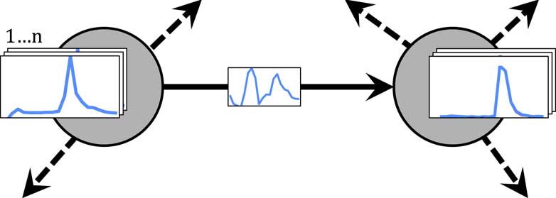
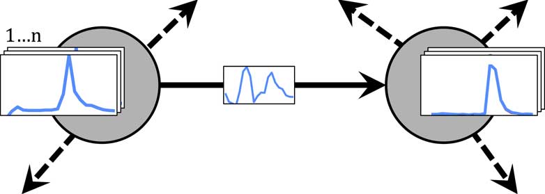
Last section discussed temporal graph analysis which lacked attribute data, whereas non-relational attribute-based time series data (Clements & Hendry, Reference Clements and Hendry1998; Croushore & Stark, Reference Croushore and Stark2001; Marcellino et al., Reference Marcellino, Stock and Watson2006) is the focus of this section. In particular, traditional time series methods ignore graph data all together (Pindyck & Rubinfeld, Reference Pindyck and Rubinfeld1981; Brockwell & Davis, Reference Brockwell and Davis2002; Ahmed et al., Reference Ahmed, Atiya, El Gayar and El-Shishiny2010; Box et al., Reference Box, Jenkins and Reinsel2013), and focus solely on modeling a time-dependent sequence of real-valued data such as hourly temperatures or economic data such as stock price or gross domestic product (Clements & Hendry, Reference Clements and Hendry1998; Croushore & Stark, Reference Croushore and Stark2001; Marcellino et al., Reference Marcellino, Stock and Watson2006). In contrast, our proposed methods naturally allow for modeling time series of attributes and graphs (i.e. relational time series data) where each node and edge may have a multi-dimensional time series with arbitrary connectivity or dependencies between them as shown in Figure 5.
Data model for relational time-series learning. Each node in the network may have an arbitrary number of time series attributes such as blood pressure, number of hourly page views, etc. Further, we also assume that each edge in the network may have an arbitrary number of time series attributes as well (not shown for simplicity). For each edge, we also model the temporal dependencies, resulting in the time series on the edge in the illustration above. As an aside, if there are multiple types of edges between nodes such as friend-edges and email-edges representing friendship between two individuals and email communications, respectively, then we would model the temporal dependencies for each of the edge types resulting in learning multiple time series of edge temporal edge strengths.
At the intersection of time series analysis and ML, Ahmed et al. (Reference Ahmed, Atiya, El Gayar and El-Shishiny2010) recently used ML methods such as Neural Networks (Hornik et al., Reference Hornik, Stinchcombe and White1989) and support vector machines (Hearst et al., Reference Hearst, Dumais, Osman, Platt and Scholkopf1998) for time series forecasting. In particular, the authors found that many of these ML methods offered significant improvements over the traditional time series models (Ahmed et al., Reference Ahmed, Atiya, El Gayar and El-Shishiny2010) such as auto-regressive models and the ilk (Brockwell & Davis, Reference Brockwell and Davis2002). The main contribution of the work by Ahmed et al. (Reference Ahmed, Atiya, El Gayar and El-Shishiny2010) was there use of traditional ML methods for time series forecasting, which has recently attracted numerous follow-up studies (Agami et al., Reference Agami, Atiya, Saleh and El-Shishiny2009; Ben Taieb et al., Reference Bengio2012; Esling & Agon, Reference Esling and Agon2012). From that perspective, our work makes a similar contribution as we formulate the problem of relational time series learning for dynamic relational graph data, and propose techniques for relational time series classification and regression, which are shown to improve over traditional relational learning and time series methods.
4.4 Relational learning
The majority of research in relational learning has focused on modeling static snapshots or aggregated data (Chakrabarti et al., Reference Chakrabarti, Dom and Indyk1998; Domingos & Richardson, Reference Domingos and Richardson2001) and has largely ignored the utility of learning and incorporating temporal dynamics into relational representations. Previous work in relational learning on attributed graphs either uses static network snapshots or significantly limits the amount of temporal information incorporated into the models. Sharan and Neville (Reference Sharan and Neville2008) assumes a strict representation that only uses kernel estimation for link weights, while genetic algorithm enhanced time varying relational classifier (Güneş et al., Reference Güneş, Çataltepe and Öğüdücü2011) uses a genetic algorithm to learn the link weights. Spatial-relational probability trees (McGovern et al., Reference McGovern, Friedland, Hay, Gallagher, Fast, Neville and Jensen2008) incorporate temporal and spatial information in the relational attributes. However, the above approaches focus only on one specific temporal pattern and do not consider different temporal granularities (i.e. they use all available snapshots and lack the notion of a lagged time-series). In contrast, we explore a larger space of temporal-relational representations in a flexible framework that can capture temporal dependencies over links, attributes, and nodes. To the best of our knowledge, we are the first to leverage the full spectrum of dynamic relational data to improve predictions.
We are also the first to propose and investigate temporal-relational ensemble methods for time-varying relational classification. However, there has been recent work on relational ensemble methods (Preisach & Schmidt-Thieme, Reference Preisach and Schmidt-Thieme2006, Reference Preisach and Schmidt-Thieme2008; Eldardiry & Neville, Reference Eldardiry and Neville2011) and non-relational ensemble methods for evolving streams (Bifet et al., Reference Bifet, Holmes, Pfahringer, Kirkby and Gavaldà2009). While none of the past work proposes temporal-relational ensemble methods for classification, there has been recent work on relational ensemble methods (Preisach & Schmidt-Thieme, Reference Preisach and Schmidt-Thieme2006, Reference Preisach and Schmidt-Thieme2008; Eldardiry & Neville, Reference Eldardiry and Neville2011). In particular, Preisach and Schmidt-Thieme (Reference Preisach and Schmidt-Thieme2006) use voting and stacking methods to combine relational data with multiple relations, whereas Eldardiry and Neville (Reference Eldardiry and Neville2011) incorporates prediction averaging in the collective inference process to reduce both learning and inference variance.
4.5 Deep learning
Our work is also related to the ML topic of deep learning (LeCun et al., Reference LeCun, Bottou, Bengio and Haffner1998; Hinton et al., Reference Hinton, Osindero and Teh2006; Marc’Aurelio Ranzato et al., Reference Marc’Aurelio Ranzato, Boureau and LeCun2007; Bengio, Reference Ben Taieb, Bontempi, Atiya and Sorjamaa2009; Lee et al., Reference Lee, Grosse, Ranganath and Ng2009; Boureau et al., Reference Boureau, Bach, LeCun and Ponce2010; Deng & Li, Reference De Raedt and Kersting2013), which has recently received a considerable amount of attention from industry due to its success in a variety of real-world applications and systems (Salakhutdinov & Hinton, Reference Salakhutdinov and Hinton2009; Lezama et al., Reference Lezama, Alahari, Sivic and Laptev2011; Couprie et al., Reference Couprie, Farabet and LeCun2013). However, nearly all of this work has focused on images and other similar types of data, whereas we focus on dynamic attributed networks. In view of our work, deep learning for dynamic relational data are informally any method that constructs a representation with varying levels of abstraction or granularity with dependencies between the various layers. For instance, the Dynamic Role Mixed Membership Model (Rossi, Reference Rossi2015) method for node prediction first learns a large set of features, then we discover roles from those features using matrix factorization (i.e. capturing the essence of that set of features), and finally we model the role transitions over time. These representations form a hierarchy of layers each capturing a different level of granularity in the dynamic attributed networks.
5 Challenges and open problems
A discussion of future challenges and directions are discussed below.
5.1 Space and time characterization
Future work should also investigate the tradeoff between space and time. Characterizing thee tradeoffs are challenging, for instance, relational time-series learning methods may learn a model using less data by considering only the most recent observations, whereas relational learning approaches, that ignore temporal information, use all available data. Moreover, modeling temporal dependencies may also lead to simpler/more accurate models, and more efficient learning and inference algorithms. However, relational time series models typically require an appropriate temporal granularity and kernel function, and learning both of these automatically may be costly.
5.2 Theoretical analysis
There has yet to be any significant theoretical analysis of the existing relational time series forecasting models, despite the fundamental importance of understanding the theoretical limitations of these models. Furthermore, future work should propose simple theoretical models that aid in the theoretical characterization of existing work.
5.3 Synthetic relational time series graphs
There have yet to be any synthetic graph models for generating relational time series graph data. However, these models would help evaluate existing approaches and characterize their limitations.
5.4 Ensemble techniques
While there has been some work in ensemble techniques for relational time series forecasting (Rossi & Neville, Reference Rossi, Gleich and Gebremedhin2012), there has yet to be any systematic investigation into the performance of these across a variety of dynamic networks. More work is needed to identify which types of dynamic networks perform best, among other characteristics.
5.5 Automatic kernel function learning
Future work should investigate the related problem of learning the kernel function automatically. While this work investigated a range of kernel functions and found the exponential to work best in most situations, we expect that for certain relational time series data, such an approach is likely to result in a significantly better predictive model. Moreover, it also makes it easier for applying the relational time series learning (for many real-world tasks), without requiring much effort on the part of the user, in terms of knowledge and assumptions about the data. However, techniques proposed in the future must address the challenges associated with the computational cost of such an approach and carefully investigate the benefits (both theoretically and empirically).
5.6 Robustness to noise
Another important problem is to investigate the ability of relational time series learning methods to handle varying levels of noise in both the relational and temporal information? Further, does modeling the temporal dependencies reduce the impact of noise, specifically, when the relational data are noisy (e.g. missing or erroneous links)?
5.7 Model selection
Selecting the appropriate relational time series model is of fundamental importance. However, there has only been a few techniques and investigations into model learning and more generally hyperparameter optimization for relational time series models (Rossi, Reference Rossi2015). Thus, more work is needed to understand the advantages and disadvantages of each approach, and new techniques developed to overcome problems and/or shortcomings of the existing work.
6 Conclusion
This paper introduces and surveys work related to the problem of relational time series forecasting. In particular, this includes the fundamental relational time series prediction tasks: (i) predicting discrete class labels (classification), and (ii) predicting a future real-valued continuous weight (regression). To that end, we introduced a unifying taxonomy that serves as a foundation for studying the main representation tasks that arise in dynamic attributed graph data (for improving relational time series forecasting). This includes the representation tasks of dynamic node and link labeling, weighting, predicting their existence, and discovering important features. Existing work is then surveyed and reinterpreted for the problem of relational time series forecasting. In particular, we discuss how these techniques, which were originally proposed for other ML tasks, can be reinterpreted and used for improving relational time series forecasting. This paper serves as a basis for investigating the important and challenging problem of relational time series forecasting.
Acknowledgements
The authors thank all the reviewers for many helpful suggestions and feedback.