1.1 Introduction to the structural and functional versatility of RNA

The RNA World hypothesis was proposed in the late 1960s as a way to explain the development of life on earth (Woese, Reference Woese1967; Crick, Reference Crick1968; Orgel, Reference Orgel1968). One of the central tenets of this hypothesis is that life emerged from self-replicating RNA molecules. Joyce & Orgel (Reference Joyce, Orgel, Gesteland, Cech and Atkins2006) articulated three basic assumptions about the RNA World: (1) genetic continuity was maintained by RNA replication, (2) Watson–Crick base pairing was the basis for replication, and (3) encoded proteins were not involved in catalysis. In other words, for any biopolymer to serve as the basis for life, it must both store information and perform diverse functions. While proteins have adapted to do the latter, organisms have no way of decoding the information they store.

It is well known that RNA can store information. For example, there are classes of viruses with genomes composed solely of single- or double-stranded RNA. However, replication as we know it depends on the presence of proteins such as RNA-dependent RNA polymerases (RDRP) or RNA-dependent DNA polymerases (RDDP) (Langland et al. Reference Langland, Cameron, Heck, Jancovich and Jacobs2006). A fundamental question then is whether RNA can replicate without protein polymerases (issues 1 and 3 above) (Joyce & Orgel, Reference Joyce, Orgel, Gesteland, Cech and Atkins2006). An attempt to address this question requires consideration of the functional versatility of RNA.

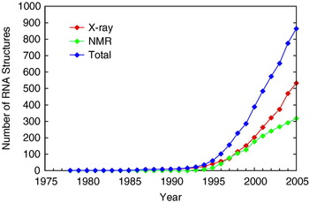
Over the course of the 40 years following the formulation of the RNA World hypothesis, a number of remarkable discoveries have been made regarding the function and structural diversity of RNA. Insight into the functional versatility of RNA begins with a survey of its structural diversity, which is covered in more detail in Section 6. Advances in X-ray diffraction methods and nuclear magnetic resonance (NMR) spectroscopy have made possible the elucidation of many RNA-containing structures (Fig. 1) (Holbrook, Reference Holbrook2005). These structures reveal that RNA adopts shapes far more complex than the aforementioned Watson–Crick duplex. At the secondary structural level, RNA forms helices with a wide range of structural defects including bulges, internal loops, hairpin loops and helical junctions (Tian et al. Reference Tian, Bevilacqua, Diegelman-Parente and Mathews2004). These secondary structures themselves often assemble into higher order tertiary structures with even greater structural complexity, including binding pockets and clefts capable of orienting substrates and binding metal ions (Doudna & Lorsch, Reference Doudna and Lorsch2005; Fedor & Williamson, Reference Fedor and Williamson2005).

Fig. 1.

Total number of publicly available RNA-containing structures. Structures were determined by X-ray crystallography (red), nuclear magnetic resonance (NMR) spectroscopy (green), or all available techniques [X-ray crystallography, NMR spectroscopy, electron microscopy and fluorescence resonance energy transfer (FRET)] (blue). The RNA structural database has grown substantially since the first tRNA structure was released (Kim et al. Reference Kim, Suddath, Quigley, Mcpherson, Sussman, Wang, Seeman and Rich1974; Robertus et al. Reference Robertus, Ladner, Finch, Rhodes, Brown, Clark and Klug1974). There was a substantial lag phase from the 1970s until 1990, followed by an exponential phase in the mid-1990s, and more recently a steep linear phase. This plot represents a wide range of folds and functions including tRNAs, rRNAs, mRNAs, transcription-related RNAs, introns, splicing-related RNAs, signal recognition particle RNAs, ribozymes, aptamers, pseudoknots, RNAs with defects such as bulges, hairpins, RNA–RNA duplexes, DNA–RNA hybrids, PNA–RNA hybrids, RNA–protein complexes, RNA–drug complexes, viral RNAs, etc. These data are available online at www.rnabase.org/metaanalysis/. We thank Professor George Rose for providing the information in this figure.

The first crystal structure of an RNA with tertiary structure – transfer RNA in the 1970s – was a revelation, as it showed that RNA could spontaneously fold into globular structures with diverse features involving both Watson–Crick and non-Watson–Crick base pairs (Kim et al. Reference Kim, Suddath, Quigley, Mcpherson, Sussman, Wang, Seeman and Rich1974; Robertus et al. Reference Robertus, Ladner, Finch, Rhodes, Brown, Clark and Klug1974). Non-Watson–Crick base pairing allows the close approach of unpaired nucleotides far apart in sequence. In addition, hydroxyl radical mapping experiments showed that catalytic RNAs have an inside and an outside (Latham & Cech, Reference Latham and Cech1989), and recent studies showed that RNA can bury up to 20% or more of its surface area in folding transitions (Conn et al. Reference Conn, Gittis, Lattman, Misra and Draper2002). Because functional versatility in RNA presupposes structural diversity, these molecular features raised the possibility that RNA might have diverse and powerful molecular recognition and catalytic functions.

The structural diversity of RNA, initially realized in tRNA, was subsequently accompanied by groundbreaking discoveries regarding its functional versatility, including demonstration that RNA can be a catalyst (Kruger et al. Reference Kruger, Grabowski, Zaug, Sands, Gottschling and Cech1982; Guerrier-Takada et al. Reference Guerrier-Takada, Gardiner, Marsh, Pace and Altman1983); development of the combinatorial methods of in vitro selection and in vitro evolution for RNA (Joyce, Reference Joyce1989; Ellington & Szostak, Reference Ellington and Szostak1990; Tuerk & Gold, Reference Tuerk and Gold1990); discovery of the regulation of gene expression by the binding of metabolites (riboswitches) (Mironov et al. Reference Mironov, Gusarov, Rafikov, Lopez, Shatalin, Kreneva, Perumov and Nudler2002; Winkler et al. Reference Winkler, Nahvi and Breaker2002), tRNAs (T-box) (Grundy et al. Reference Grundy, Rollins and Henkin1994) and small micro RNAs (miRNA) directly to the RNA (Lau et al. Reference Lau, Lim, Weinstein and Bartel2001; Matzke & Birchler, Reference Matzke and Birchler2005); determination of the complex three-dimensional structures of many functional RNAs alone and in complex with proteins (Holbrook, Reference Holbrook2005); and solving the structure of the ribosome, which suggested that it is a ribozyme (Carter et al. Reference Carter, Clemons, Brodersen, Morgan-Warren, Wimberly and Ramakrishnan2000; Nissen et al. Reference Nissen, Hansen, Ban, Moore and Steitz2000; Harms et al. Reference Harms, Schluenzen, Zarivach, Bashan, Gat, Agmon, Bartels, Franceschi and Yonath2001; Yusupov et al. Reference Yusupov, Yusupova, Baucom, Lieberman, Earnest, Cate and Noller2001). These and many other discoveries illustrated the diversity of functional roles played by non-coding RNAs (ncRNAs) (e.g. tRNA, rRNA, UTRs, introns, and miRNAs).

In recent years, there has been a tremendous increase in the number of RNA structures determined (see Fig. 1 for details). In particular, X-ray diffraction methods have greatly advanced to provide numerous complex RNA structures (Holbrook, Reference Holbrook2005). This is attributable to improved methodologies for the production and manipulation of RNAs, as well as advances in the crystallography of RNA (Cate & Doudna, Reference Cate and Doudna2000; Golden & Kundrot, Reference Golden and Kundrot2003; Rupert & Ferre-D'Amare, Reference Rupert and Ferre-D'amare2004). The new structures span a wide range of RNA functions, allowing RNA function to be discerned in molecular terms. Throughout this article, we attempt to organize the functional and structural diversity in terms of simple models.

1.2 Rationale for model-making

One goal of this article is to organize discoveries in the context of simple models. Given the complexity of RNA structure and function, this may seem contradictory. However, there are several good reasons to build minimalist models. The most fundamental reason is to try to understand what is essential for a certain function. The models dictate the necessary states of the system and the ways in which the population of these states must be controlled by external stimuli – typically the binding of ligands or alteration of RNA sequence. An additional reason to make models is that even simple models are often associated with fairly complex and unanticipated functions, which can have biological ramifications (Dill & Bromberg, Reference Dill and Bromberg2003). Finally, it is hoped that the models will provide practical frameworks for describing and organizing experimental observations made on functional RNAs.

It is not the intention of this article to summarize the literature on any particular area of RNA function or to be exhaustive in the details of one given function. Instead, the intention is to determine what states and equilibria are essential for a given behavior, and to do so in a largely biopolymer-independent fashion. We then judge whether RNA possesses the chemical diversity needed to achieve that function. A second goal is to provide the basic tools such that investigators can create their own models, derive equations, and perform simulations.

2.1 Model-making as a molecular process

We choose to take a molecular approach to model-making because this permits functions to be described in terms of chemical or physical changes and accommodates effects of changes in sequence on function (e.g. Bevilacqua, Reference Bevilacqua2003). Once a functional model is written down, statistical thermodynamics can be used to generate the partition function. The partition function leads to phenomenological constants – observed and functional constants – that can be defined in terms of elementary chemical descriptors including intrinsic rate constants, microscopic ligand equilibrium constants, secondary structure stability and ligand concentration. We attempt to gain insight into a given behavior by simulating derived functional constants. Granted, many of the models are too simple to capture the intricacies of cellular function, but simulations of the models do exhibit many of the necessary components of complexity; as such, they begin to establish plausibility of a simple RNA-based form of life.

There are numerous functions that an informational biopolymer must perform in order to support life. We divide these into chemical and physical changes. Chemical changes are those that involve the making and breaking of covalent bonds, for example replication, transcription, translation, and metabolism. Physical changes are those that involve conformational switches and non-covalent binding of another molecule and are involved in regulating chemical changes such as those mentioned above. Crucial to physical changes are specificity and the ability to make decisions in response to inputs from the environment. Typically, the stimulus is recognition of a ligand, which often occurs non-covalently but can be covalent.

Decision-making processes, described as logic gates, are often related to performing simple logic operations by response to multiple stimuli, or inputs. For example, during replication a decision must be made as to which nucleotide to add opposite a templating base. Thus, while a biopolymer must have a functional state capable of carrying out covalent chemical changes, regulation of the activity of this state by population changes is equally important and contributes much to the complexity of life. The ability of a biopolymer to modulate the fraction of active molecules in response to a stimulus leads to the notion of functional ‘constants’, which are not really constants but complex expressions defined in terms of elementary descriptors. As such, functional ‘constants’ vary in response to environmental perturbations such as changing ligand concentration and sequence; this makes them interesting from a biological perspective, but means they are complex and best understood by simulation.

2.2 Model-making: a three-step process

We begin with an overview of the three-step process used in model-making. The three steps involve writing down a minimal model, deriving equations from the model and then simulating the behavior. The simulations are related to functional constants in the equations and generally show how the function depends on ligand concentration.

2.2.2 Step 2: Deriving equations

The second step in the model-making process is deriving equations from the model. The functional constant, k _func, is defined as a fractional value of the intrinsic rate constant, k _intr. This arises because we have connected N to one or more non-functional M states. k _func and k _intr are related by the simple equation

(1)

where f _N is the fraction of molecules in the native state (Bevilacqua, Reference Bevilacqua2003; Bevilacqua et al. Reference Bevilacqua2003). The important point is that changes in behavior (represented here by an apparent rate constant, k _func) arise from changes in population (f _N) rather than changes in the value of k _intr, that is from physical changes rather than chemical ones. If some perturbation to the system (e.g. a mutation or a change in ligand concentration) does not result in an appreciable change in the population of native state molecules, then function does not change. Two of the assumptions of this model are that all of the states are in rapid equilibrium and that chemical changes are irreversible. Clearly, these are limiting behaviors, and in this sense capture only part of the functional complexity of RNA; reversible chemical changes and kinetic control, known to occur in RNA biology, would only serve to further increase functional complexity.

A major goal of this step in the process is to define the functional constant, which captures the behavior of the system, in terms of ligand concentration and microscopic equilibria constants, which often depend on biopolymer sequence in simple ways such as nearest-neighbor models. In all cases, a partition function is used as an efficient way to treat f _N. The equation can be viewed as the intermediary in the model-making process, with the most valuable insight typically gained from testing how additions to or subtractions from the model affect simulated behavior.

3.1 Scheme 1: A simple chemical change

The simplest functional model is shown in Scheme 1. Only two states are depicted, the functional state N and the product state P, and they are connected by an arrow with rate constant k _intr. The transformation here is a chemical change and could involve making or breaking a bond in a biopolymer, or making a natural product or metabolite. There is no substrate shown binding to N, which is a literal interpretation of a self-cleaving ribozyme or a depiction of a multiple-turnover enzyme operating at saturation. The major limitation of this scheme with regards to biology is that there is no means to respond to input from the environment, that is regulation is not possible.

Scheme 1.

A simple chemical change.

3.2 Scheme 2: A modulated chemical change

In order to have regulation, we need an additional state, M, that must be incapable of carrying out chemistry; for example, M could have a misfold that compromises the integrity of the active site. The functional model in Scheme 2 depicts this scenario, in which M is connected to N by a reversible equilibrium governed by the microscopic equilibrium constant, K _M/N=[M]/[N], and M is non-reactive; that is there is no direct access to P from M. The presence of M depopulates N. This behavior is captured by Eq. (2.1) in which the functional rate constant, k _func, is a fractional value of k _intr, as determined by the multiplier f _N. The expression for f _N in terms of K _M/N is given in Eq. (2.4), which is derived from the concentration of the functional state, N, divided by the sum of the concentrations of all the states the molecules populate, in this instance N and M [Eq. (2.2)]. N is chosen as a reference state and used to divide the numerator and denominator of the expression for f _N to give Eq. (2.3).

Scheme 2.

Modulated chemical change.

The denominator of Eq. (2.4) is the partition function, Q, of the system [Eq. (2.5)]. This partition function is the summation of two terms, each of which reflects one of the states preceding chemistry, N and M. As such, the first term in Q is the numerator of the expression for f _N. We point out the relationship between f _N and Q because Q is useful for deriving additional species plots simply by putting the term(s) for the state(s) of interest in the numerator.

As seen in Eq. (2.6), as K _M/N increases, reflecting an increase in the population of molecules that are misfolded, k _func decreases. K _M/N might increase, for example, due to a mutation that favors the stability of a structural element present in M but not N. Alternatively, if the relative population of M and N is sensitive to another variable such as temperature or ionic strength, then the k _func might display a dependence on these variables. While the misfolding depicted in Scheme 2 does provide a way to attenuate function, the obvious limitation of Scheme 2 with regards to biology is that there is no rapid way for the system to respond to the varying levels of complex stimuli from the environment.

3.3 Scheme 3: Negative feedback

The next functional model (Scheme 3) corrects for the shortcoming of inability to rapidly respond to environmental changes by having a ligand, L (e.g. a metabolite), bind to M but not N, which results in feedback inhibition loop. This repression is the simplest and most common form of gene regulation, as it keeps a gene product from becoming toxic by binding to its own gene and turning it off (Tucker & Breaker, Reference Tucker and Breaker2005). In prokaryotes the binding event is typically upstream of the gene of interest (i.e. in the 5′-UTR), while in eukaryotes it is often in introns or the 3′-UTR (Sudarsan et al. Reference Sudarsan, Barrick and Breaker2003). This type of feedback is depicted in the functional model in Scheme 3, which is an extension of Scheme 2, in which L binds to M but not N to give a stable complex, ML. The equilibrium between M and ML is governed by a new microscopic equilibrium constant, K _ML,intr=[M][L]/[ML]. We choose to write this as a dissociation constant (units of M), and note the difference between true equilibrium constants (denoted herein as ‘microscopic’ or ‘intrinsic’ constants) and those observed in actual experiments (K _ML,obs). The new state ML, like M, is non-reactive (i.e. no arrow connecting ML to P). In the simplest case, the structural basis for lack of chemistry by ML would be the same as for M, and binding of L serves to block conversion of M to N, thereby increasing the population of M-containing states. Therefore, the presence of ML allows depopulation of N in response to ligand concentration in the cell. The ML state leads to an additional term in the partition function, Q [Eq. (3.4)].

Scheme 3.

Ligand-modulated chemical change/negative feedback.

According to the simulation in Scheme 3, ligand binding downregulates function by depopulating N. As such, we can expect the fractional population of N to be significant (i.e. near unity) at very low concentrations of ligand, that is K _M/N⩽0·1. The dependence of f _N on the concentration of L can be described according to a simple hyperbolic response [Eq. (3.5)], which leads to limiting equations for f _max and K _ML,obs in terms of microscopic constants, Eqs (3.6) and (3.7), respectively.

Equation (3.7) has two interesting implications. First, for small values of K _M/N, the observed dissociation constant is larger (i.e. weaker binding) than the intrinsic dissociation constant by a factor of 1/K _M/N [Eq. (3.7)]. This is captured in the simulations in Scheme 3, which were carried out according to Eq. (3.3). As K _M/N is decreased from 10 to 0·001, the dissociation constant K _ML,obs observed in the parametric plots shifts to progressively higher values, represented as the inflection point of the sigmoidal curves in the upper simulation. Importantly, the simulations show that the response of the biopolymer to ligand concentration can be altered by changes in the sequence away from the site of ligand binding; that is the observed ligand affinity K _ML,obs is tuned by changing the ligand-free equilibrium constant, K _M/N. The implications for this phenomenon on evolvability will be considered later in the article (see Section 8.1). Second, when K _M/N is ⩾0·1 the fraction of native molecules is noticeably less than 1 in the absence of ligand [Eq. (3.6)]; moreover, under these conditions, the observed dissociation constant, K _ML,obs, approaches its minimal value of K _ML,intr and then becomes essentially unresponsive to the value of K _M/N [Eq. (3.7)]. The low population of native molecules under high K _M/N conditions is why it was suggested that N would be significantly favored over M in the absence of ligand (i.e. K _M/N≪1).

3.4 Scheme 4: Positive feedback

In some cases, a positive feedback loop may be desirable. For example, a toxin might direct biosynthesis of a secondary metabolite, or a metabolite might turn on a set of genes involved in its own catabolism. Development of positive feedback is handled in a relatively straightforward manner, as shown in Scheme 4. In contrast to Scheme 3, K _N/M is now expected to be less than 1 because the default state is with the gene turned off; decreasing K _N/M keeps ‘leaky’ expression in the absence of ligand activator to a minimum (note that we switch from K _M/N in Scheme 3 to K _N/M in Scheme 4 to allow the equations to be developed in a parallel fashion). Ligand L is now assigned to bind the native state N rather than M. The new state NL, like N, is capable of carrying out chemistry (i.e. arrow connecting NL to P) that is captured in Eq. (4.1) by having two terms rather than one in the numerator. In the simplest case, the structural basis for NL being able to perform chemistry is the same as for N, and binding of L blocks spontaneous conversion of N to M, thereby increasing the population of N-containing states. In contrast to Schemes 2 and 3, we chose M as the reference state (Eq. 4.3) in order to work in terms of K _N/M. According to the simulation in Scheme 4, ligand binding now upregulates function by populating reactive NL. In a manner paralleling Scheme 3, the dependence of f _N and f _NL on the concentration of L can be described according to a simple hyperbolic response [Eq. (4.6)], which leads to limiting equations for f _min and K _NL,obs in terms of microscopic constants, Eqs (4.7) and (4.8) respectively.

Scheme 4.

Ligand-modulated chemical change/positive feedback.

As with Eq. (3.7), Eq. (4.8) leads to two related conclusions. First, the observed binding affinity, K _NL,obs, can be tuned weaker than the intrinsic value simply by decreasing the ligand-free M and N equilibrium constant, K _N/M. As in Scheme 3, this behavior illustrates that the response of the biopolymer to ligand concentration can be tuned by changes in sequence away from the site of ligand binding. Second, when K _N/M is ⩾0·1, the fraction of native molecules in very low concentrations of ligand is appreciably greater than zero [Eq. (4.7)]; moreover, under these conditions, the observed dissociation constant, K _NL,obs, approaches its minimal value of K _NL,intr and then becomes essentially unresponsive to the value of K _N/M [Eq. (4.8)]. This high population of native molecules is why it was suggested that M would be significantly favored over N in the absence of ligand (i.e. K _N/M≪1).

At this point, several general conclusions can be made regarding Schemes 3 and 4. First, the ability to have appreciable fold-regulation in response to ligand concentration requires that the system sacrifice some of its binding affinity (i.e. K _d,obs>K _d,intr) in order to favor population of the appropriate ligand-free state in the absence of ligand. Second, this phenomenon is especially important for a positive feedback scheme. For example, if we define fold-regulation as f _N+NL([L]=100×K _d,obs)/f _N+NL([L]=0·01×K _d,obs), then when K _N/M (or K _M/N)=1, regulation is only ∼2-fold for Scheme 4, but ∼100-fold for Scheme 3 [for the case of negative regulation in the preceding section (Scheme 3), fold-regulation is defined as the inverse of this ratio]. In other words, negative regulation is ∼50 times greater than positive regulation for a modest ligand-free equilibrium of 1. Likewise, when K _N/M (or K _M/N)=0·1, regulation is ∼10-fold for Scheme 4, but is still ∼100-fold for Scheme 3. Thus, even when the ligand-free equilibrium favors the ligand-free state by a factor of ∼10, regulation is ∼10 times greater for negative than positive regulation. These striking differences can be attributed to tighter control of the off state in negative regulation for intermediate values of K _M/N. To achieve large fold-effects for positive regulation, N must be significantly depopulated in the absence of ligand, that is by having very small K _N/M values. But this comes at a cost, namely weaker observed binding of L. If the biopolymer has limits on its intrinsic ability to bind a small molecule, then at some point the observed K _d will no longer be physiologically relevant.

3.5 Scheme 5: Specificity in binding

In general, a given metabolite in the cellular milieu will be in the presence of many closely related metabolites. As such, it is crucial that binding be specific to ligand L over other ligands. We consider specificity by modification of Scheme 3 for negative feedback as it appears to be more common than positive feedback and to permit greater fold-regulation; however, similar arguments can be readily extended to Scheme 4. Scheme 5 adds to Scheme 3 an additional equilibrium between M and a competing non-cognate ligand, L′, which is governed by a new microscopic equilibrium constant, K _ML′,intr. This leads to a partition function, Q, with a fourth term reflecting the new ML′ state [Eq. (5.4)].

Scheme 5.

Ligand-modulated chemical change/negative feedback/specificity.

It is the relative population of ML and ML′ given by the ratio of terms 3 and 4 in Q that governs specificity. This leads to the following definition for specificity as it relates to Scheme 5.

(6)

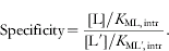
This expression parallels the widely used definition of specificity for two competing substrates derived from Michaelis–Menten kinetics in which specificity is determined by the ratio of the k _cat/K _M values multiplied by the ratio of substrate concentrations (Fersht, Reference Fersht1985). The difference with Eq. (6) is that there is no k _cat term. This is because, according to Scheme 5, the L- and L′-bound enzymes are non-reactive.

One important conclusion reached from analysis of Scheme 5 is that the ligand-free equilibrium between N and M, K _M/N, does not enter into Eq. (6). Thus, it is only the intrinsic affinities of the enzyme for L and L′ that are important for specificity. In addition, it is not the ratio of the concentrations of L and L′ that dictate specificity, but the ratio of the [L]/K _d ratios. As such, an enzyme must adapt its binding site to discriminate against L′, perhaps using steric exclusion to increase K _ML′,intr, until the term in the denominator of Eq. (6) is small relative to the numerator. As a corollary, if the denominator in Eq. (6) is already small, perhaps because [L′] is small in vivo, then there will be no selective pressure on the enzyme for such discrimination against this ligand and it may bind tightly to the enzyme.

5.1 Scheme 6: AND gate

The AND gate gives a correct output, in this case some function, only when both A and B are present. This logic is shown in the truth table contained within Scheme 6 (in all cases an input/output is signified with a ‘1’ and absence of an input/output with a ‘0’). Using the example of DNA replication again, this positive feedback mechanism might be important in a polymerase that depends on both a regulatory unit and the correct NTP. This system requires two binding sites and function to arise only when both sites are filled, and could involve an allosteric change in which binding of both ligands unmasks an active site.

5.2 Scheme 7: OR gate

The OR gate gives a correct output when either A or B (or both) are present. This logic is shown in the truth table in Scheme 7. This might be the case if an operon contains genes that help to synthesize a precursor common to two different metabolites, A and B. In this case, output could be activation of a repressor of the synthesis of A and B. Scheme 7 presents two possible OR gates. In Scheme 7a there are separate binding sites for A and B, much like for Scheme 6 except that filling either (or both) site(s) leads to function. Scheme 7b shows a simpler scenario in which there is a single binding site that accommodates A or B, which is reasonable if A and B are related at the molecular level.

5.3 Scheme 8: NOR gate

The NOR gate gives a correct output only when neither A nor B is present. This logic is shown in the truth table in Scheme 8. As with the OR gate, two schemes can be envisioned (Schemes 8a and 8b). In Scheme 8a, A and B can bind separately or together. Scheme 8b shows the simpler scenario in which there is a single binding site that accommodates A or B.

5.4 Scheme 9: NAND gate

Lastly, the NAND gate gives a correct output when either A or B, or when neither, is present; it gives no output only when both A and B are present (Scheme 9). This logic is shown in the truth table in Scheme 9. As with the AND gate, this system would involve separate binding sites for A and B. The two sites could communicate with each other such that binding of both A and B induces a conformational change inhibiting activity. Alternatively, there could be duplication of active sites giving rise to two closely related enzymes, in which each enzyme operates independently of the other. In this case, A could inhibit enzyme 1 and B could inhibit enzyme 2, and thus both A and B would have to be present to completely lose activity.

6.1 Functional group diversity

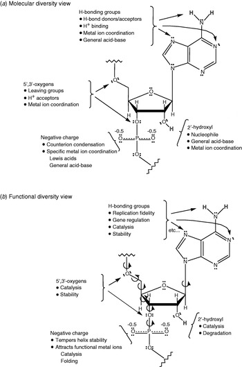
As shown in Fig. 2a, the functional groups in RNA can engage in a wide range of interactions. The nucleobases have carbonyl, amino, and imino functional groups, which can participate in hydrogen bonding, proton transfer, and metal ion coordination, and thereby increase overall structural diversity. Imino nitrogen pK _as for G and U are ∼9·2 and for A and C are 3·5–4·2 (Fig. 3). These differences clearly define hydrogen-bond acceptor–donor roles, which facilitate molecular recognition. The bases can also participate in metal ion coordination, especially at non-Watson–Crick positions, which have unusual geometries and additional functional groups for metal ligands. The ribose sugar likewise has lone pairs on the 2′-, 3′-, 4′- and 5′-oxygens that can accept hydrogen bonds and coordinate metal ions. In addition, the 3′- and 5′-oxygens can act as leaving groups if properly facilitated, and the 2′-hydroxyl can act as a nucleophile. This latter trait makes RNA much more reactive than DNA because nucleic acids, being polyanions, are generally uninviting to most nucleophiles (Blake, Reference Blake2005). High reactivity is the bane of RNA as it makes it unstable; however, it also greatly simplifies catalysis, as an exogenous nucleophile does not have to be recruited (although it sometimes is), as well as permits rapid turnover of RNA levels in gene expression. The phosphodiester moiety provides additional metal ion coordination, which can lead to Lewis and Brønsted acid behavior, as well as additional structural diversity (Fig. 2) (DeRose, Reference Derose2003). Overall, there are many more hydrogen bond acceptors than donors in RNA, which are responsible for the attraction of metal ions to RNA. Finally, there are many dihedral angles in RNA (on average ∼7/nt; Fig. 2b), which affords the flexibility needed to adopt diverse conformations. Thus, even though RNA contains only four fairly similar nucleobases, it can engage in myriad interactions providing the potential for profound catalytic rate enhancements.

Fig. 2.

Annotated RNA structure. (a) Repeating unit in RNA. Highlighted is the molecular diversity of RNA. (b) Highlighted is the functional diversity of RNA. Dihedral angles are shown.

Fig. 3.

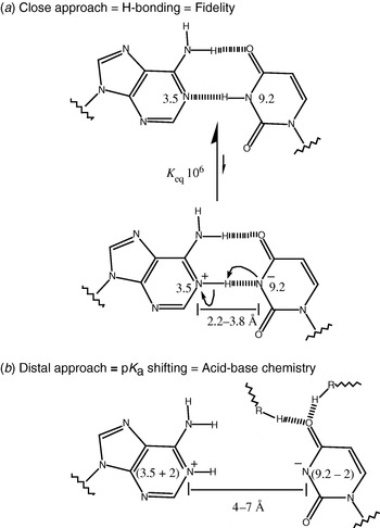
(a) Molecular basis of fidelity. Hydrogen bonding is unique and prototropic shifts shown in panel b are disfavored. (b) pK _a shifting due to electrostatics. Bases are drawn sufficiently separated, perhaps due to tertiary bonds, to preclude hydrogen bonding but to still experience a favorable electrostatic attraction.

Of course there are limitations to RNA, especially when compared to proteins. The unperturbed pK _as of the nucleobases are far from neutrality and the nucleobases have no especially good nucleophiles. This contrasts sharply with amino acids such as histidine, which has a pK _a near 7, and cysteine, which has a good nucleophile in the thiolate. In addition, RNA enzymes may not be efficient in excluding water from their active sites; RNA folding does not seem to be driven by the hydrophobic effect, suggesting much of the water is not driven from the structure (Bloomfield et al. Reference Bloomfield, Crothers and Tinoco2000; McKay et al. Reference Mckay, Haptonstall and Gellman2001). These differences may limit dramatic rate acceleration phenomena which typically require conditions very different from those free in solution.

Next, we consider how the molecular diversity of RNA imparts functional versatility. As shown in Fig. 2b, each of the functional groups in RNA can be associated with particular chemical and physical transformations. The hydrogen-bonding groups impart replication fidelity, gene regulation, catalysis and thermodynamic stability through interactions with proteins or other nucleic acids. Moreover, the 5′- and 3′-oxygens participate in phosphodiester transesterification reactions, while the 2′-hydroxyl is a prime participant in catalysis and RNA degradation. The negative charge tempers duplex stability, largely because of repulsion between the two strands, and also attracts functional metal ions that participate in catalysis and folding. In the context of an RNA World, this characteristic might have been important in the spontaneous dissociation of a newly synthesized strand from its template before the emergence of helicases.

Figure 3 shows possibilities for less obvious molecular diversity in RNA. The standard Watson–Crick recognition between A and U, with the bases in their standard protonation states, is shown in Fig. 3a. The population of the imino proton-transferred species is generally thought to be less than 1 ppm on the basis of the difference in pK _as (3·5–9·2). However, if the bases are sufficiently separated such that hydrogen bonding cannot take place (>4 Å) (e.g. positioned by the tertiary framework) but are close enough that electrostatic attraction can still be experienced (<7 Å), then they might influence each other's pK _a and lead to shifting (Fig. 3b). On the basis of model compounds, shifts on the order of 2 pK _a units could be accomplished for distances of 3 bonds (Cantor & Schimmel, Reference Cantor and Schimmel1980; Fersht, Reference Fersht1985); this is similar to the distances expected between general acid–base participants in phosphodiester bond cleavage, given a trigonal bipyramidal transition state (Rupert et al. Reference Rupert, Massey, Sigurdsson and Ferre-D'amare2002). Lastly, the presence of equal number of bases with high imino proton pK _as (G and U) and low pK _as (A and C) may have permitted RNA to buffer itself around neutrality before sophisticated buffering schemes evolved helping to stabilize it.

6.2 Secondary structural diversity

As mentioned in Section 5, RNA can switch between various conformations with alacrity. Given the wide range of secondary structural elements available to RNA, conformational switching can have profound functional consequences. Secondary structure provides the foundation for more complex tertiary structure, while having important biological function in its own right. One example is the use of secondary structures to control gene expression through a riboswitch expression platform (Mandal & Breaker, Reference Mandal and Breaker2004b). The structural changes that occur upon binding typically sequester or uncover a sequence of regulatory importance, such as the Shine–Dalgarno sequence or a hairpin–poly(U) stretch that can serve as a terminator. These significant cellular processes are modulated largely through simple hairpin structures in which a single-strand of RNA folds back onto itself and forms Watson–Crick base pairs. The single-stranded loop portion of the hairpin also forms a network of tertiary interactions that vary according to loop sequence (Mathews & Turner, Reference Mathews and Turner2006).

The simplest RNA secondary structure is the perfectly base-paired dsRNA duplex, wherein each base is correctly matched to its Watson–Crick partner on an opposite anti-parallel strand. The formation of Watson–Crick base pairs provides RNA the ability to store information and repress gene expression (Matzke & Birchler, Reference Matzke and Birchler2005). A double-stranded portion of RNA may also have internal loops wherein opposing bases do not Watson–Crick base pair; such loops may persist for several bases within a helix. The number of mismatched bases in the 5′- and the 3′-strand may be the same (symmetric) or different (asymmetric), giving rise to even greater molecular diversity. In many cases, multiple hairpin loops can form off one large internal loop, resulting in crevices ideal for ligand binding and structural rearrangements (Montange & Batey, Reference Montange and Batey2006; Serganov et al. Reference Serganov, Polonskaia, Phan, Breaker and Patel2006; Thore et al. Reference Thore, Leibundgut and Ban2006).

An additional factor that adds complexity to RNA secondary structure is the formation of non-canonical base pairs, such as wobble bases and mismatches (Tian et al. Reference Tian, Bevilacqua, Diegelman-Parente and Mathews2004; Mathews & Turner, Reference Mathews and Turner2006). Taking into consideration the many combinations of the secondary structure elements that can occur, it becomes apparent that RNA secondary structure can be extraordinarily complex. Moreover, because of the degeneracy of base pairing, multiple structures with similar free energy can occur. An important consequence of such competing secondary structures is the ability to effect different functions vis-à-vis RNA refolding events. Stabilization of any given secondary structure through events such as ligand binding can preferentially populate a state having catalytic activity, or perhaps turn off such activity. This idea is discussed more fully in Section 7.2.

6.3 Tertiary structural diversity

Even though many of the nucleobases of a structured RNA have their Watson–Crick faces sequestered in base pairs (i.e. the functional groups that make the nucleobases unique are not available for higher order interactions), RNA can still use other functional groups to engage in tertiary interactions including the minor groove edges and Hoogsteen face of the bases, the 2′-hydroxyl and 4′-oxygen of the ribose sugar, and the phosphoryl oxygens. Here, we give a brief overview of the diversity of RNA tertiary structures known. The RNA tertiary interactions that have been discovered and characterized to date can be divided into several classes: coaxial helices, A-minor motifs, kissing hairpins, pseudoknots, ribose zippers, tetraloop–receptor interactions, and loop–loop interactions (tRNA) (reviewed in Leontis & Westhof, Reference Leontis and Westhof2003; Holbrook, Reference Holbrook2005; Lemieux & Major, Reference Lemieux and Major2006; Leontis et al. Reference Leontis, Lescoute and Westhof2006).

Coaxial helices form when nucleobases from two separate helices stack, forming a pseudo-continuous helix. These are highly stabilizing tertiary interactions and have been found in a number of RNAs, including tRNA (Shi & Moore, Reference Shi and Moore2000), RNase P (A- and B-types) (Krasilnikov et al. Reference Krasilnikov, Yang, Pan and Mondragon2003, Reference Krasilnikov, Xiao, Pan and Mondragon2004), the P4–P6 domain of the group I intron (Cate et al. Reference Cate, Gooding, Podell, Zhou, Golden, Kundrot, Cech and Doudna1996), and the hammerhead (Scott et al. Reference Scott, Finch and Klug1995) and HDV ribozyme (Ferre-D'Amare et al. Reference Ferre-D'amare, Zhou and Doudna1998). The ‘A-minor motif’ involves the insertion of the minor groove edges of As into the minor groove of neighboring helices, where they form hydrogen bonds with one or more 2′-hydroxyl group, and can occur in four different ways. These motifs have been found in RNase P (B-type) (Krasilnikov et al. Reference Krasilnikov, Yang, Pan and Mondragon2003) and in group I introns (Adams et al. Reference Adams, Stahley, Kosek, Wang and Strobel2004; Guo et al. Reference Guo, Gooding and Cech2004; Golden et al. Reference Golden, Kim and Chase2005). ‘Kissing hairpins’ form when base pairing occurs between the single-stranded residues of two hairpin loops. These have been found in viral RNAs (Chang & Tinoco, Reference Chang and Tinoco1997), 23S ribosomal RNA (Schlunzen et al. Reference Schlunzen, Zarivach, Harms, Bashan, Tocilj, Albrecht, Yonath and Franceschi2001), a group I intron (Golden et al. Reference Golden, Kim and Chase2005), and the adenosine-responsive riboswitch (Serganov et al. Reference Serganov, Yuan, Pikovskaya, Polonskaia, Malinina, Phan, Hobartner, Micura, Breaker and Patel2004). ‘Pseudoknots’ form when bases pair between nucleotide loops (hairpin or internal) and bases outside the enclosing loop. Because pseudoknots bring together preformed regions of the RNA, they tend to enforce a compact topology, which is crucial to forming active sites and binding crevices. Pseudoknotted structures can be catalytic as in the case of the HDV ribozyme (Ferre-D'Amare et al. Reference Ferre-D'amare, Zhou and Doudna1998), Tetrahymena group I intron (Adams et al. Reference Adams, Stahley, Kosek, Wang and Strobel2004; Guo et al. Reference Guo, Gooding and Cech2004; Golden et al. Reference Golden, Kim and Chase2005), and the in vitro selected Diels–Alder ribozyme (Serganov et al. Reference Serganov, Keiper, Malinina, Tereshko, Skripkin, Hobartner, Polonskaia, Phan, Wombacher, Micura, Dauter, Jaschke and Patel2005). In addition, pseudoknotted structures occur in the RNA component of human telomerase (Theimer et al. Reference Theimer, Blois and Feigon2005), in viruses that use them to induce frameshifts during the translation of viral proteins (Shen & Tinoco, Reference Shen and Tinoco1995; Egli et al. Reference Egli, Minasov, Su and Rich2002; Nixon et al. Reference Nixon, Rangan, Kim, Rich, Hoffman, Hennig and Giedroc2002), and in binding regions of aptamers (Nix et al. Reference Nix, Sussman and Wilson2000; Sussman et al. Reference Nix, Sussman and Wilson2000) and riboswitches (Montange & Batey, Reference Montange and Batey2006; Serganov et al. Reference Serganov, Polonskaia, Phan, Breaker and Patel2006; Thore et al. Reference Thore, Leibundgut and Ban2006). A ‘ribose zipper’ forms when consecutive hydrogen-bonding interactions occur between ribose 2′-hydroxyl groups from different regions of an RNA chain or between RNA chains, and can take on 11 possible forms (although only seven forms have been found so far). They have been found in a number of RNAs, including the hairpin (Rupert & Ferre-D'Amare, Reference Rupert and Ferre-D'amare2001), HDV (Ferre-D'Amare et al. Reference Ferre-D'amare, Zhou and Doudna1998) and hammerhead ribozymes (Scott et al. Reference Scott, Finch and Klug1995), RNAse P (A- and B-types) (Krasilnikov et al. Reference Krasilnikov, Yang, Pan and Mondragon2003, Reference Krasilnikov, Xiao, Pan and Mondragon2004), and group I introns (Adams et al. Reference Adams, Stahley, Kosek, Wang and Strobel2004; Guo et al. Reference Guo, Gooding and Cech2004; Golden et al. Reference Golden, Kim and Chase2005). In sum, RNA can form a remarkably wide range of tertiary structures that are responsible for diverse ligand binding and catalytic functions.

7.1 Suitability of RNA for Scheme 1: A simple chemical change

In Scheme 1, a simple chemical transformation is shown. This scheme is an oversimplification because most reactions are regulated in vivo; however, this aspect is accommodated below. RNA has been shown to carry out a wide range of chemical reactions. Naturally occurring ribozymes perform phosphodiester cleavage and ligation reactions (e.g. HDV ribozyme and group I introns), as well as peptidyl transfer (e.g. the ribosome) (Doudna & Lorsch, Reference Doudna and Lorsch2005). Additionally, through in vitro approaches RNA has been shown to be capable of catalyzing many other reactions including carbon–carbon bond formation and Diels–Alder reactions (Tarasow et al. Reference Tarasow, Tarasow and Eaton1997).

Beginning with tRNA and following with group I introns, small ribozymes and culminating in the ribosome, RNA has been shown to adopt a variety of shapes (Holbrook, Reference Holbrook2005). Moreover, the number of structures continues to increase rapidly, as illustrated in Fig. 1. Folding of RNA is largely hierarchical, with secondary structural elements folding independently and assembling into complex tertiary folds. As discussed, the secondary elements themselves are diverse. It is the apposition of these elements and interaction of imperfections that give rise to diverse molecular interactions and chemical catalysis.

RNA possesses most of the catalytic devices necessary for catalysis (Narlikar & Herschlag, Reference Narlikar and Herschlag1997; Bevilacqua et al. Reference Bevilacqua, Brown, Nakano and Yajima2004; Doudna & Lorsch, Reference Doudna and Lorsch2005; Fedor & Williamson, Reference Fedor and Williamson2005). Shortly after RNA enzymes were discovered, it was shown that RNA could have an inside and an outside, just like protein enzymes, which opened the possibility for active site clefts (Latham & Cech, Reference Latham and Cech1989). Metal ions can stabilize charge development in transition states (DeRose, Reference Derose2003) and nucleobases have been implicated in general acid–base catalysis (Bevilacqua et al. Reference Bevilacqua, Brown, Nakano and Yajima2004), often with shifted pK _as. Rate acceleration by RNA catalysts of up to 10¹¹-fold over the uncatalyzed reaction have been reported (Narlikar & Herschlag, Reference Narlikar and Herschlag1997). Moreover, the nucleobases themselves have been shown to contribute on the order of 10⁶-fold to rate acceleration (Bevilacqua et al. Reference Bevilacqua, Brown, Nakano and Yajima2004). Thus, RNA has the molecular potential to be a potent catalyst.

7.2 Suitability of RNA for Scheme 2: A modulated chemical change

In addition to rate acceleration, a biopolymer that forms the basis for life must be capable of being regulated. Scheme 2 shows a modulated chemical change, which requires both a functional state, N, and a non-functional state M. RNA is extremely adept at adopting multiple folds, some of which are inactive, as in M. The conformational flexibility of RNA arises because of degeneracy in base pairing. RNA has only four side-chains and, counting GU and AC wobbles, half of the 16 possible pairs are compatible with an A-form geometry. Thus, RNA can readily adopt different conformations with similar free energies. Examples include conformational switching of terminator–anti-terminator helices found in bacterial gene regulation (Babitzke, Reference Babitzke1997) and alternative pairing regions in ribozymes (Cao & Woodson, Reference Cao and Woodson1998; Pan & Woodson, Reference Pan and Woodson1998; Chadalavada et al. Reference Chadalavada, Knudsen, Nakano and Bevilacqua2000). RNA is capable of fine-tuning regulation by simple changes in secondary structure. For example, a GC to GU point mutation can incur a free energy penalty of 1·5 kcal/mol (Mathews et al. Reference Mathews, Sabina, Zuker and Turner1999; Turner, Reference Turner, Bloomfield, Crothers and Tinoco2000), or a factor of ∼10 in an equilibrium constant at 37°C, making changes in populations of secondary structures, and thus adjustments in regulation, facile. Such changes can also affect population of functional tertiary structures, if folding is cooperative (Blose et al. in press). Finally, we note that RNA can form structures with extreme stability. For example, Turner & Bevilacqua (Reference Turner, Bevilacqua, Gesteland and Atkins1993) discussed half-lives for unfolding of simple helices on the order of millions of years for a simple 8 bp duplex, although it is highly temperature dependent. Thus, there are times when RNA will be under kinetic control instead of thermodynamic control, such as described by Wickiser et al. (Reference Wickiser, Cheah, Breaker and Crothers2005a, Reference Wickiser, Winkler, Breaker and Crothersb), suggesting that temperature may play a key role in regulation (Turner & Bevilacqua, Reference Turner, Bevilacqua, Gesteland and Atkins1993). These additional levels of complexity serve to further enhance the diversity of regulatory schemes available to RNA. However, Scheme 2 is limited in that there is no response to complex external stimuli, as discussed earlier.

7.3 Suitability of RNA for Scheme 3: Negative feedback

In Scheme 3, the population of N is negatively regulated by the concentration of a ligand, for example a metabolite that is the product of a gene or operon. Can RNA adopt the states shown in Scheme 3? As discussed for Schemes 1 and 2, RNA can adopt native states, N, capable of forming product P, as well as inactive states M. The ability of RNA to bind a ligand L was first demonstrated in vitro with selection, or SELEX, experiments. Pioneering work from the Gold, Szostak, and Joyce laboratories demonstrated that RNA could bind small molecules with typical affinities in the nM to μM range (Joyce, Reference Joyce1989; Ellington & Szostak, Reference Ellington and Szostak1990; Tuerk & Gold, Reference Tuerk and Gold1990). Such RNAs were dubbed ‘aptamers’, from the Latin ‘aptus’ for ‘to fit’ (Ellington & Szostak, Reference Ellington and Szostak1990).

More recently, aptamers have been found to occur in nature, and have been termed ‘riboswitches’. Indeed, at least 4% of the Bacillus subtilis genome is thought to be regulated through cis-acting regulatory RNAs, indicating that riboswitches comprise a common and important type of regulatory element (Winkler, Reference Wickiser, Winkler, Breaker and Crothers2005). In most cases, the riboswitches undergo a conformational change upon ligand binding, which is equivalent to the N to ML switch shown in Scheme 3. Indeed, Breaker and co-workers have shown that riboswitches can have a modular construction consisting of an ‘aptamer platform’ (the M to ML binding transition in Scheme 3) and an ‘expression platform’ (the M to N conformational transition in Scheme 3) (Tucker & Breaker, Reference Tucker and Breaker2005). The M to N equilibrium can be a terminator–anti-terminator switch for transcriptional control, or an SD–anti-SD switch (SD is the Shine–Dalgarno sequence, which is a purine-rich set of nucleotides that base pair with rRNA to initiate translation in prokaryotes) for translational control (Babitzke, Reference Babitzke1997). Moreover, the aptamer platform, in the absence of the expression platform, binds small molecules tighter. For example, for the negatively regulated thiamine pyrophosphate (TPP) riboswitch, the aptamer platform alone binds TPP 20-fold tighter than the full-length riboswitch (Winkler et al. Reference Winkler, Nahvi and Breaker2002). According to Eqs (3.5)–(3.7), this argues for a K _M/N of about 1/20, or that the N state is ∼95% populated in the absence of TPP.

7.4 Suitability of RNA for Scheme 4: Positive feedback

In Scheme 4, the population between N and M is positively regulated by the concentration of ligand. There are examples of this behavior in riboswitches as well; for example, the adenine, guanine, and glycine riboswitches (Mandal & Breaker, Reference Mandal and Breaker2004a; Mandal et al. Reference Mandal and Breaker2004). Indeed, the glycine riboswitch has been shown to bind two equivalents of glycine, with the first binding event favoring the second by 100- to 1000-fold; this enhancement is at least as great as that observed in oxygen binding by hemoglobin, arguing that RNA can effect protein-like cooperative enhancements (Mandal et al. Reference Mandal and Breaker2004). Nonetheless, there are currently many fewer examples of classes of positively regulated riboswitches than negatively regulated ones (Nudler & Mironov, Reference Nudler and Mironov2004; Tucker & Breaker, Reference Tucker and Breaker2005; Winkler, Reference Wickiser, Winkler, Breaker and Crothers2005). This could be attributed to several factors. First, from a genetic perspective the most commonly needed type of control may be repression. Once a gene product is abundant, there is a distinct need to stop making more of it to avoid toxic behavior or wasting of cellular building blocks. Second, the level of fold-regulation achievable for positive control does not approach the level for negative control, as discussed in Section 3. Third, the number of well-characterized riboswitches is small at present and upregulators could be overlooked to date.

7.5 Suitability of RNA for Scheme 5: Specificity in binding

The issue of specificity is addressed in Scheme 5. A few examples illustrate that aptamers and riboswitches can be highly specific. The classic demonstration of specificity is the theophylline aptamer, in which affinity for theophylline over the related ligand caffeine is 10 000-fold (Jenison et al. Reference Jenison, Gill, Pardi and Polisky1994). This discrimination is remarkable given that the two ligands differ only by the presence of one extra methyl group on caffeine. Discrimination was explained at the molecular level by steric exclusion of the larger caffeine (Zimmermann et al. Reference Zimmermann, Jenison, Wick, Simorre and Pardi1997). A later study showed that the only stable interaction between caffeine and the theophylline aptamer (detected by NMR) is the stacking of the drug with the terminal base pair of the RNA, and that the core structural elements of the aptamer only form when theophylline is present, suggestive of a cooperative folding mechanism (Zimmermann et al. Reference Zimmermann, Wick, Shields, Jenison and Pardi2000).

In the case of riboswitches, the TPP riboswitch shows remarkable specificity, discriminating against thiamine phosphate and thiamine by more than 1000-fold. Recent crystal structures reveal that this riboswitch engulfs its products and engages in crucial interactions (Montange & Batey, Reference Montange and Batey2006; Serganov et al. Reference Serganov, Polonskaia, Phan, Breaker and Patel2006; Thore et al. Reference Thore, Leibundgut and Ban2006). In another instance, crystal structures of the A-riboswitch (add mRNA aptamer from Vibrio vulnificus, which binds adenine) bound to adenine, and G-riboswitch (xpt mRNA aptamer from B. subtilis, which binds guanine) have been solved (Batey et al. Reference Batey, Gilbert and Montange2004; Serganov et al. Reference Serganov, Yuan, Pikovskaya, Polonskaia, Malinina, Phan, Hobartner, Micura, Breaker and Patel2004). These riboswitches adopt similar global structures and the purine binding pockets are identical except for one nucleotide – a U for the A-riboswitch and a C for the G-riboswitch. Remarkably, the A-riboswitch can be converted to a G-riboswitch by simply mutating the U to a C, and similarly a G-riboswitch can be converted to an A-riboswitch by mutating the C to a U (Mandal & Breaker, Reference Mandal and Breaker2004a). In these cases, discrimination between binding of guanine and adenine has been recently determined by Batey and co-workers to be remarkably large, at ∼50 000-fold (Gilbert et al. Reference Gilbert, Stoddard, Wise and Batey2006). Thus, riboswitches appear to show greater specificity towards their cognate metabolite than their in vitro aptamer counterparts.

According to Eq. (6), the affinity differences reflect differences in the intrinsic K _ds. Interestingly, the molecular basis for discrimination appears to be different in each case. Unlike the theophylline aptamer, where the poor binding analyte was larger, in the TPP aptamer the poor binding analytes are smaller. This indicates that RNA can achieve specificity by both antideterminants and positive determinants, including the somewhat surprising recognition of anionic functionalities (e.g. pyrophosphate).

7.6 Suitability of RNA for Schemes 6–9: Involvement in logic gates

The logic gates depicted in Schemes 6–9 are built up from the pieces in Schemes 1–5. As such, demonstration of the feasibility of Schemes 1–5 indirectly establishes the feasibility of Schemes 6–9. Some striking examples of logic gates have been reported for both DNA- and RNA-based systems. For instance, Stojanovic and co-workers have constructed NOT, AND, and XOR gates through a modular design that combines molecular beacon stem-loops and antisense oligonucleotides with hammerhead-type deoxyribozymes (Stojanovic et al. Reference Stojanovic, Mitchell and Stefanovic2002). Using related approaches, these authors recently constructed a full-adder, which is a logic element used in computer engineering to perform arithmetic (Lederman et al. Reference Lederman, Macdonald, Stefanovic and Stojanovic2006). Kolpashchikov & Stojanovic (Reference Kolpashchikov and Stojanovic2005) demonstrated that these DNA enzyme-based logic gates could also be used to control the functional state of aptamers. This advance is exciting as it has the potential to lead to the development of therapeutic devices; for example, delivering a drug only when certain disease markers are present. Penchovsky & Breaker (Reference Penchovsky and Breaker2005) have made advances along these lines in logic gates and therapeutic devices for ribozyme-based logic gates. They developed a computational algorithm to design hammerhead ribozymes that respond to multiple oligonucleotide inputs, and whose oligonucleotide-cleavage outputs can trigger the activity of other, downstream logic gates.

In sum, the series of states and transformations depicted in Schemes 1–9 have all been demonstrated to varying extents in vitro, and many have already been discovered in vivo. In the same way that logic gates are built up from the pieces of Schemes 1–5, polymerases and other complex RNA-based machines can be built up from the logic gates in Schemes 6–9. Thus, demonstration of the feasibility of these schemes indirectly establishes feasibility of more complex RNA function. Although non-trivial, establishing such complexity is chemically possible and requires correct ‘engineering’ of the above pieces. Lastly, we mention that the preceding illustrations are not intended to try to illustrate any superiority of RNA over proteins for carrying out specific, complex biological functions, but are only meant to illustrate that RNA has the potential to perform most of the basic functions essential for the emergence of life at a tolerable level. In the next section, we ask whether the ability to carry out these basic functions, along with the molecular architecture of RNA, offers RNA any advantages in terms of emergence of life.

8.1 Evolvability of RNA

One important characteristic for a polymer in an early life form is the ability to readily evolve new functions and adapt to changing conditions (Wagner, Reference Wagner2005). The ability of RNA to adopt multiple conformations makes it possible that two conformations of the same sequence, which might have related but somewhat different tertiary structures, could have unique functions. For example, Schultes & Bartel (Reference Schultes and Bartel2000) showed that a single RNA sequence could switch between a class III self-ligating and an HDV self-cleaving ribozyme by means of a single mutation. Forconi & Herschlag (Reference Forconi and Herschlag2005) have also suggested a role for promiscuous background reactions in providing access to new functions in catalytic RNAs. Although not shown explicitly in Schemes 3 and 4, the M state might have novel, albeit poor, chemical activity, which could provide a simple entrée to new function by evolution. Because the fractional populations of M and N lie between 0 and 1 in the absence of ligand, the probability for such processes is non-zero.

Schemes 3 and 4 also suggest that RNA is well suited for adapting to changing environmental conditions. As discussed in Section 3, observed ligand affinity can be tuned by changes in the sequence of secondary structural elements away from the tertiary elements involved in ligand binding or catalysis. Indeed, Herschlag and co-workers have shown the importance of binding interactions away from the site of catalysis in affecting hammerhead and group I ribozyme activity (Narlikar et al. Reference Narlikar, Gopalakrishnan, McConnell, Usman and Herschlag1995; Hertel et al. Reference Hertel, Peracchi, Uhlenbeck and Herschlag1997). As illustrated in the Scheme 3 simulation, the K _M/N equilibrium constant modulates observed ligand affinity, and because K _M/N is a ligand-free constant it can be changed by simply strengthening or weakening base pairing. In principle, this provides a facile path to adaptation. For example, a mutually exclusive terminator–anti-terminator pairing could undergo a point mutation resulting in a GU to GC change (worth up to a factor of 10 in the equilibrium constant) (Mathews et al. Reference Mathews, Sabina, Zuker and Turner1999), exclusively stabilizing the anti-terminator and thereby weakening observed ligand binding. Notably, specificity is also not a function of K _M/N [Eq. (6)], arguing that the riboswitch should not alter its specificity for the cognate ligand upon such mutagenesis. The converse, changes within a ligand binding site or an enzyme active site, provides other possible ways of tuning the observed binding constant, but they may perturb the very function of the M or N state or alter specificity. In addition, binding site changes typically require multiple mutations, presumably making them infrequent events. For example, Guo et al. (Reference Guo, Gooding and Cech2006) found that three of the mutations that stabilize the Tetrahymena ribozyme were in fact destabilizing when present as single-site changes. The ability for RNA to adapt to changing conditions by simple changes in base pairing strength may be a reason why RNA is so evolvable (Blose et al. in press).

8.2 Cooperativity in general acid–base catalysis

The four nucleobases are extremely adept at molecular recognition. Watson–Crick base pairing is the basis for storage of genetic information in the helical structures of DNA and RNA. As discussed in Section 1, absence of a ‘base pairing’ in proteins leads to the inability to decode the very genetic information contained within proteins, which limits their utility in an emergent form of life. Unfortunately, the same molecular features that make RNA excellent for storing and decoding information limit its functional versatility. Of prime importance is the lack of functional groups with pK _as near neutrality. Fortunately, much like proteins, the structural complexity of RNA confers heterogeneous microenvironments capable of pK _a perturbation to neutrality. We have discussed this phenomenon previously and divided pK _a shifting down into two classes (Bevilacqua et al. Reference Bevilacqua, Brown, Nakano and Yajima2004). Here we simply state that pK _a shifting is possible and that it can have several distinct molecular origins. It can arise from cooperativity in folding, or because of a local electrostatic pocket of high potential (Moody et al. Reference Moody, Lecomte and Bevilacqua2005). In particular, separation of two bases with low and high imino proton pK _as (e.g. A and G with pK _as of 3·5 and 9·2, respectively) outside of Watson–Crick base pairing distance can lead to the potential for electrostatic coupling (Fig. 3b). This can help to populate rare zwitterionic states of RNA that might be functional for acid–base chemistry, as in the case of the hairpin ribozyme (Rupert et al. Reference Rupert, Massey, Sigurdsson and Ferre-D'amare2002; Bevilacqua, Reference Bevilacqua2003).