2.1. Dirt cones on the Kuskulana Glacier

Our survey of the Kuskulana Glacier explored the region above ∼900 m elevation along the main glacier trunk. The upper extent of our survey region reached ∼1400 m elevation. As stated previously, two prominent clean-ice bands extended down-glacier before becoming completely debris-covered by ∼1100 m elevation. The northern ice band formed an elevated ridge with a large supraglacial stream on its southern side. The southern clean-ice band, however, formed a shallow trough. The trough began at the confluence of a northwest-flowing tributary glacier at 1400 m elevation and extended west for ∼4 km before becoming completely debris-covered. In the ice trough, the glacier undergoes lateral shear in flow. We noted the presence of marginal (chevron) crevasses and little topographic relief within the ice trough relative to the hummocky, debris-covered topography tens-of-meters to the north. Numerous supraglacial streams flowed down and across the trough. These streams terminated into crevasses and moulins.

We recorded the GPS locations of 9 dirt cones on the southern ice trough of the Kuskulana Glacier and 15 large moulins (∼1–4 m diameter at glacier surface) within and adjacent to the trough (Fig. 2). All positions were recorded with a Garmin inReach handheld GPS. These GPS coordinates were used to approximate the elevations of each dirt cone using the 5 Meter Alaska Digital Elevation Model, published with the USGS 3DEP Data Collection. Glacier surface velocities at each dirt cone were generated using auto-RIFT and approximated using the NASA MEaSUREs ITS_LIVE project (Gardner and others, Reference Gardner, Fahnestock and Scambos2024).

2.2. Surveys and observations

We undertook detailed surveys of five dirt cones and recorded observations of four additional cones. For each survey, we photographed the cones from all sides to document the cone geometry. We then excavated a narrow trench parallel to the cone slope to document debris properties and to measure debris thickness. The purpose of the debris thickness measurements was to quantify the range of debris thicknesses found on dirt cones for the purpose of comparing to model output. When possible, debris thickness measurements were made at the top, middle and base of the cone. However, thick debris often made it impossible for us to measure debris thickness at more than a single point. Debris layer thickness was measured using a centimeter graded ruler printed in a field notebook cover. The distributions of debris grain sizes on each dirt cone were visually approximated in the field using a Wentworth grain size chart.

We measured the cone slopes to determine if/when the debris surface slope approximates the underlying ice surface slope. Ice surface slopes were measured directly by removing the surface debris and placing the flat edge of a Suunto PM5/360PC Clinometer against the ice. At least one direct measurement of ice surface slope was recorded for each cone we surveyed. These measurements showed that ice surface slopes are approximately equal to the debris surface slope. However, measuring the ice surface slope was only possible in places where the debris layer was thin enough that we could remove the debris from ice surface without it immediately becoming re-buried by debris up-slope. The debris surface slopes were measured from photographs in ImageJ. For each image, the cone slope angles were measured relative to the horizontal orientation of the images on both sides of the cone profile. To reduce biases in these measurements, between 7 and 14 slope angles were measured for each cone using at least five different photographs captured from different aspects of each cone. Only images of cones completely within the center of the field of view were used to limit the influence of lens distortion.

2.2.2. DC-4

DC-4 was the largest dirt cone (∼6 m tall) we observed on the Kuskulana Glacier (Fig. 3). It was located at an elevation of 1200 m, where the glacier flows ∼10 m/y. DC-4 was much longer than it was wide, forming an elevated ridge. The dirt cone ridge ran parallel to a nearby marginal crevasse with an actively draining moulin. The region surrounding DC-4 was generally debris covered; however, there were patches of bare ice with drainage runnels on the northern and southern sides. The debris covering DC-4 was notably lighter in color and the clasts significantly more rounded than the surrounding debris. Boulders surrounded the base and lower slopes of DC-4.

Figure 3.

The largest dirt cone we observed on the Kuskulana Glacier (DC-4). A long, low ridge of debris connected to the cone (from lower right to center). This debris ridge was parallel to nearby crevasses. The debris covering this cone was lighter in color and more rounded than surface debris nearby.

The debris covering DC-4 was much thicker at the apex than the base. Debris at the cone apex exceeded 0.5 m, and we were not able to excavate deep enough to reach the ice surface at these points before the trenches re-filled with debris. The debris at the base of the south face of this dirt cone was 0.15 m. The debris covering the cone was composed of coarse sand and rounded cobbles and pebbles. The ice surface slope at the base was 25^∘ and the median debris surface slope was 28.4^∘.

2.3. Summary of observations

The dirt cones on the Kuskulana Glacier developed along and adjacent to a band of clean ice. Crevasses and moulins were observed in close proximity to the dirt cones. The cones ranged in height from <0.1 m to more than 3 m in height and formed pointed apexes or sharp ridges. In contrast to the angular clasts and unsorted sediment that surrounded the dirt cones, the sediment atop and at the bases of dirt cones was rounded and stratified by grain size. The median debris slopes ranged from 28^∘ to 40^∘ and ice slopes ranged from 25^∘ to 45^∘ (Fig. 4). Debris thicknesses on the cones varied significantly between cones, ranging from 0.01 m to thicknesses >0.5 m.

Figure 4.

Mean slopes of dirt cones on the Kuskulana Glacier. Slopes were measured from photographs of each cone using ImageJ.

3.1. Conceptual model

Based on our observations, we infer that the dirt cones on the Kuskulana Glacier developed from fluvially deposited debris in crevasses and moulins, as described by Agassiz and Bettannier Reference Agassiz and Bettannier(1840). Figure 5 illustrates this process. We speculate plunge pools form via vertical drilling when supraglacial streams drain into crevasse/moulins (Covington and others, Reference Covington, Gulley, Trunz, Mejia and Gadd2020). Glacier advection and the opening of new crevasses causes some of these moulins to be abandoned, leaving a sediment deposit within the ice. Melt progressively lowers the glacier surface, eventually transforming the relict plunge pool into a debris-filled pit at the glacier surface. Finally, as Agassiz and Bettannier Reference Agassiz and Bettannier(1840) described, cone development commences as differential melt causes the debris-filled pit to gain relief relative to the surrounding bare ice. The rounded clasts and sediment sorting we observed atop the cones strongly suggest fluvial debris transport. However, the only strict requirement for this conceptual model is a concentration of sediment within a pit or crevasse surrounded by faster-melting ice.

Figure 5.

The Agassiz model of dirt cone development, extended to encompass debris deposition in moulins. As supraglacial streams flow into moulins/crevasses, they create plunge pools that trap sediment. Moulins become abandoned as the glacier advects, leaving a debris-filled pit within the ice. Melt eventually lowers ice surface to the debris pit. Differential melt leads to the development of a dirt cone.

In the field, we observed moulin/crevasse depths to be on the order of ∼10–30 m. Glacier speeds where the dirt cones were present are ∼20 m/y (Fig. 2). Although there are no reported surface lowering rates on the Kuskulana Glacier, surface lowering at similar elevations on the nearby Kennicott Glacier are ∼1–3 m/y (Anderson and others, Reference Anderson, Armstrong, Anderson and Buri2021). Therefore, we infer that the abandoned moulins likely advected ∼60–600 m before dirt cone emergence. The time required for a dirt cone to fully develop after emergence depends on the initial volume of sediment, the melt rate and the debris diffusion rate. Quantitatively examining the development of dirt cones from a debris-filled pit at the ice surface is the focus of the remaining sections.

3.2. Mathematical model

We developed a mathematical model to explore the dynamics of dirt cone growth and controls on cone geometry. In the following section, the relevant equations are presented and a dimensionless model is derived. The numerical implementation of this model incorporates two advancements in modeling topographic evolution on debris-covered glaciers: (1) it simulates topographic evolution in two dimensions and (2) it removes a simplifying assumption used in other models that requires gradients in debris thickness to be small (e.g. Moore, Reference Moore2021). With the model, we examine the influence of bare ice melt rate, debris diffusivity and sediment volume on the development of dirt cones. The results help guide understanding of how glacier dirt cones and, more generally, topographic relief develops through differential melt.

Debris thickness, h, controls the ice ablation rate, $\partial s/\partial t$, on debris-covered glaciers. Although a very thin debris layer ( $ \lt \sim3$ cm) increases melt rates relative to bare ice (Östrem, Reference Östrem1959), it is common to approximate sub-debris melt with a hyperbolic model (Anderson and Anderson, Reference Anderson and Anderson2016; Reference Anderson and Anderson2018; Mölg and others, Reference Mölg, Ferguson, Bolch and Vieli2020; Moore, Reference Moore2021):

(1)\begin{equation} \frac{\partial s}{\partial t} = -b_0 \frac{h_\mathrm{c}}{h_\mathrm{c} + h} \;, \end{equation}

where b ₀ is the bare-ice melt rate, s is the ice surface elevation and $h_\mathrm{c}$ is an empirically derived characteristic debris thickness that scales how rapidly melt rates decrease as debris thickness increases (Anderson, Reference Anderson2000).

Sediment flux on debris-mantled glacier hillslopes depends on slope and the debris thickness. Terrestrial landscape evolution models simulate hillslope debris flux as a diffusion process that can depend either linearly (Gilbert, Reference Gilbert1909; Perron and others, Reference Perron, Dietrich and Kirchner2008) or nonlinearly (Andrews and Bucknam, Reference Andrews and Bucknam1987; Roering and others, Reference Roering, Kirchner and Dietrich2001; Perron, Reference Perron2011) on topographic slope. Nonlinear models force a rapid increase in flux as hillslopes approach a critical slope, $S_\mathrm{c}$. Slope-stability models (Moore, Reference Moore2018) and observations (Nicholson and others, Reference Nicholson, McCarthy, Pritchard and Willis2018) showed that slopes on debris covered glaciers become increasingly unstable and prone to failure as hillslopes steepen. Furthermore, the widespread development of ice cliffs on debris-covered glaciers exemplifies a threshold steepness where ice slopes can no longer support a debris layer. This supports the use of a nonlinear debris flux model for debris-covered glaciers.

Similar to Moore Reference Moore(2021), we employ an expression for nonlinear debris flux (Andrews and Bucknam, Reference Andrews and Bucknam1987; Roering and others, Reference Roering, Kirchner and Dietrich2001) and modify it to account for a finite-thickness debris layer:

(2)\begin{equation} Q = -D(1-\mathrm{e}^{-h/h_\mathrm{D}})\frac{\nabla z}{1-\left(\frac{|\nabla z|}{S_\mathrm{c}}\right)^2} \;, \end{equation}

where D is the debris diffusivity. The topographic surface, z, is defined as the sum of debris thickness and ice elevation. In the dirt cone model, nonlinear flux keeps the cone slopes from becoming unrealistically steep. Here, $h_\mathrm{D}$ is a characteristic thickness for debris diffusion, where diffusion rates rapidly decline when debris thins below this depth. When $h\gg h_\mathrm{D}$, debris thickness does not substantially influence debris flux. The critical debris thickness in Eqn (2) should be small enough to ensure diffusion rates are not too low when debris is thick, while still allowing flux to go to zero as the debris layer thins. We follow Moore Reference Moore(2021) and assume that both critical debris thicknesses are approximately the same. In all model runs explored here, and in the equations below, we set $h_\mathrm{D}=h_\mathrm{c}$.

From conservation of mass, the time rate of change in debris thickness along a hillslope is

(3)\begin{equation} \frac{\partial h}{\partial t} = D\nabla \cdot \left[(1-\mathrm{e}^{-h/h_\mathrm{c}})\frac{\nabla z}{1-\left(\frac{|\nabla z|}{S_\mathrm{c}}\right)^2}\right] \;. \end{equation}

When evaluating the divergence, previous models on debris-covered glaciers assumed that debris flux is dominated by topographic slope (Anderson, Reference Anderson2000; Moore, Reference Moore2021). Although this assumption is reasonable for relatively uniform debris layers, it does not account for steep gradients in debris thickness that do not follow the topographic slope, such as debris-filled pits in the ice surface. In our implementation of this model, we allow for spatial gradients in debris thickness to influence debris flux, keeping $1-\mathrm{e}^{-h/h_\mathrm{c}}$ within the divergence operation.

The sum of Eqns (1) and (3) gives the time rate of change in topographic elevation:

(4)\begin{equation} \frac{\partial z}{\partial t} = -b_0 \left(\frac{h_\mathrm{c}}{h_\mathrm{c} + h}\right) + D \nabla \cdot \left[(1-\mathrm{e}^{-h/h_\mathrm{c}})\frac{\nabla z}{1-\left(\frac{|\nabla z|}{S_\mathrm{c}}\right)^2} \right] \;. \end{equation}

We scale this equation using the characteristic debris depth, $h_\mathrm{c}$, and an initially undefined characteristic length scale, $\ell$:

\begin{equation*} h = h_\mathrm{c}h^*\quad \nabla = \frac{\nabla^*}{\ell}\quad z = \ell z^*\quad t = \frac{\ell}{b_0} t^* \;. \end{equation*}

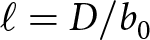
After scaling, it becomes natural to define the length scale as $\ell = D/b_0$. This length scale is similar to the characteristic hillslope length utilized in landscape evolution models (Roering and others, Reference Roering, Kirchner and Dietrich2001; Perron, Reference Perron2011). In our case, $\ell$ approximates the distance at which horizontal debris diffusion rates are matched by vertical lowering rates from melt. At distances greater than $\ell$ from the debris source, melt processes will dominate. Putting it all together, we have the dimensionless model

(5)\begin{equation} \frac{\partial z^*}{\partial t^*} = -\frac{1}{1 + h^*} + \nabla^* \cdot \left[(1-\mathrm{e}^{-h^*}) \frac{\nabla^* z^*}{1-\left(\frac{|\nabla^* z^*|}{S_\mathrm{c}}\right)^2} \right]\; . \end{equation}

When $h\gg h_\mathrm{c}$, sub-debris melt is negligible ( $(1+h^*)^{-1}\rightarrow 0$). Thus, if debris is thick, the debris diffusion term dominates changes in surface elevation. As the debris thins ( $h^*\rightarrow 0$), diffusion rates slow because $1-\mathrm{e}^{-h^*}\rightarrow 0$, thus sub-debris melt plays an increasingly important role in changes in elevation.

Since Eqn (5) is a function of both $z^*$ and $h^*$, we need a second equation to specify the system. To obtain this, we convert Eqn (1) into dimensionless form, using $s=\ell s^*$ and $s=z-h$, which leads to

(6)\begin{equation} \frac{\partial z^*}{\partial t^*} - \frac{h_c b_0}{D} \frac{\partial h^*}{\partial t^*} = -\frac{1}{1+h^*}. \end{equation}

4.1. Time-dependent behavior

First, we examine cone development through time. These experiments demonstrate the ability of the model to produce dirt cones from debris-filled pits and allow us to examine cone development through time. Each simulation begins with a debris-filled pit with diameter 0.5 m and we examine the cones that develop from pits with three different depths: 0.25, 0.5 and 1.0 m. We track the ice surface elevation (s), debris thickness (h), topographic elevation (z) and mean cone slope to better understand how a debris-filled pit undergoes topographic inversion as it evolves into a dirt cone. For these experiments, all parameter values are held constant to demonstrate the basic model behavior ( $b_0 = 0.04$ m d⁻¹, D = 0.005 m² d⁻¹, $h_\mathrm{c} = 0.08$ m and $S_\mathrm{c} = 1.15$). In this and all subsequent experiments, cone height (z ^’) refers to the height of the cone apex relative to the bare ice surrounding the base of the cone. Ice height (s ^’) refers to the height of the ice surface at the cone apex relative to the bare ice near the base of the cone.

4.2. Debris volume and cone height

In the second set of experiments, we investigate how debris volume influences cone height. We vary both the pit depths and radii. We allow the cones to grow until the debris thickness at the apex $h' \lt 0.01$ m. All parameter values are held constant ( $b_0 = 0.04$ m d⁻¹, D = 0.005 m d⁻¹, $h_\mathrm{c} = 0.08$ m and $S_\mathrm{c} = 1.15$) to focus on the relationship between debris volume and cone height.

4.3. Controls on cone geometry

In the third set of experiments, we investigate how the length scale $\ell= D/b_0$ and the critical slope $S_\mathrm{c}$ influence cone development. We vary $\ell$ by varying the diffusion constant (D) and the bare ice melt rate (b ₀) across the range of reasonable values (Table 1). Twenty-five simulations, each with a unique value for $\ell$, were run for three values of the critical slope $S_\mathrm{c} =$ 0.9, 1.15 and 1.4. All simulations begin with a circular, debris-filled pit 0.5 m wide and 0.5 m deep, with $h_\mathrm{c} = 0.8$ m. These experiments allow us to derive empirical equations that relate $\ell$ to the cone height and mean slope.

These simulations demonstrate that cone geometry is controlled by $\ell = D/b_0$, not the specific value of D or b ₀. To more clearly illustrate this and to show why $\ell$ controls cone geometry, we simulate cone development from ‘infinitely’ deep pits of debris. The deep pits eliminate the influence of decreasing debris supply on cone development and render sub-debris melt at the cone apex negligible. The infinite pit experiments begin with debris-filled pits 100 m deep and with 0.5 m diameters. We examined three characteristic lengths in two sets of three simulations. In the first set, we set the melt rate at $b_0 = 0.04$ m d⁻¹, calculate diffusion rates to give the characteristic lengths $\ell = 0.0025, 0.0125, 0.025$ m and run the simulations for 30 days (equivalent to 1.2 m of bare ice melt at the cone base). In the second set of simulations, we set the melt rate at $b_0 = 0.03$ m d⁻¹ and calculate new diffusion rates to again give the characteristic lengths $\ell = 0.0025, 0.0125, 0.025$ m. We run these simulations for 40 days to again allow 1.2 m of bare ice melt. In both sets of simulations, a quasi-steady-state cone form emerges. From this, we gain a better understanding of how $\ell$ controls cone geometry.

5.1. Time-dependent behavior

Figure 7 shows the development of a dirt cone from a debris-filled pit 0.5 m in diameter and 0.5 m deep after 0, 18 and 36 days. As melt lowered the ice surface surrounding the debris-filled pit, debris diffused away from the pit and onto the surrounding ice, forming the slopes of the emerging cone. The cone grew in width and height until the debris supply at the apex was exhausted (Fig. 7).

Figure 7.

An example simulation of cone development from a debris-filled pit 0.5 m wide and 0.5 m deep. The shade of gray corresponds to the debris thickness. Black indicates debris thicker than $h_\mathrm{c} = 0.08$ m. (a) The simulation begins with a circular pit of debris. (b) After 18 days, a cone has formed with the debris-filled pit at the cone apex. (c) After 36 days, the pit has exhausted its debris supply, inverted, and the cone is covered in a thin layer of debris.

Figure 8a shows cone and ice surface transects for the simulation as shown in Figure 7. The transects illustrate how differential melt and debris diffusion from the pit produced a cone nearly 0.5 m tall and more than 2 m wide. In this experiment, the bottom of the pit inverts (i.e. has a greater elevation than the pit edge) after 27 days of cone development. Figure 8b illustrates the change in debris thickness on the cone slope through time. On the slope outside of the pit, debris thickness decreased down slope in the early stages of cone growth. As debris thickness at the apex continued to decrease, debris thickness at the base of slope eventually becomes greater than at the cone apex. Debris thickness on the cone slopes, outside of the pit, never exceeded ∼0.08 m during this simulation. Figure 8c shows how cone slope changed during development. The cone slope steepened quickly above the pit and became steepest at the edge of the pit. Cone slope then decreased with distance from the edge of pit.

Figure 8.

Time slice transects depicting cone development from a debris-filled pit 0.5 m wide and 0.5 m deep (b ₀ = 0.04 m d⁻¹, D = 0.009 m d⁻¹, $h_\mathrm{c}$ = 0.08 m, $S_\mathrm{c}$ = 1.15). (a) Time slices of the ice surface elevation (blue) and the debris surface (black) every 12 days. The bare-ice surface surrounding the pit melts more rapidly than the debris-filled pit, causing the cone to emerge. As cone height increases, the debris diffuses down-slope and widens the cone. (b) Time slices of debris thickness at 12 day intervals. Debris is exhumed from the pit and transported down slope as it undergoes topographic inversion. (c) Time slices of the cone slopes at 12 day intervals. The slope magnitude is greatest across the edge of the pit. For (a), (b) and (c), the cone apex is at the 0.0 m position.

Figure 9 illustrates cone development from a 0.5 m diameter pit and three debris depths: 0.25 m (Fig. 9a,d,g), 0.5 m (Fig. 9b,e,h) and 1.0 m (Fig. 9c,f,i). The first row of plots (Fig. 9a,b,c) shows cone height (z ^’), ice height (s ^’) and debris thickness (h ^’) at the apex. Deeper debris-filled pits produced taller dirt cones. Debris thickness at the apex decreased as the cone heights increased until the simulations were stopped when $h'=0.01$ m. Figure 9d, e and f show the rates of change of ice height, debris thickness and cone height at the apex, relative to the surrounding bare ice. A thin vertical line marks the time of pit inversion. For the 0.25 m deep pit (Fig. 9a,d,g), pit inversion occurred 15 days after the simulation began. For the 0.5 m (Fig. 9b,e,h) and 1.0 m (Fig. 9c,f,i) deep pits, pit inversion occurred after 27 and 48.5 days, respectively.

The initial pit depth controls the melt rate at the cone apexes (Fig. 9d,e,f, solid blue lines). Deeper pits, with correspondingly greater debris depths, resulted in faster cone growth because of the lower melt rate at the cone apex. When debris thickness at the apex $h' \lt 0.2$ m, the rate of change in ice height decreased rapidly. This debris thickness corresponds to a melt rate between one-half and one-third of the bare ice melt rate. Finally, the cone growth rates approached zero as debris thicknesses at the apex approached zero.

Figure 9.

Cone development from three pit geometries. Each column corresponds to a single pit depth. Pit depths increase left to right: 0.25 m, 0.5 m and 1.0 m. The pit radius was 0.25 m. Each column shares the same horizontal axis. Plots (a), (b) and (c) depict the debris thickness at the cone apex (h ^’, gray dash-dot line), cone height (z ^’, black dashed line) and ice height at the cone apex (s ^’, blue line). The left axes are cone/ice height and the right axis is debris depth. Simulations were stopped when the debris depth at the cone apex $h' \lt 0.01$ m. Plots (d), (e) and (f) show the rate of change in ice height, debris thickness and cone height at the apex as a functions of time. The time when the debris pit inverts is marked with a thin vertical line. Plots (g), (h) and (i) show the mean cone slopes (2× height/width). Cone slope decreased when the debris thickness at the cone apex was less than the debris thickness on the slopes.

The rate of change in debris thinning rate ( $\partial h'/\partial t$) at the cone apex begins at zero and becomes increasingly negative as the cone emerged (Fig. 9d,e,f, dash-dot orange lines). The more negative the debris thinning rate at the apex, the faster debris moves away from the cone apex. After the initial decrease, the pit depth influenced the debris thinning rate as the cones develop. For the shallowest 0.25 m deep pit (Fig. 9d), the debris thinning rate decreased until the pit inverted, then increased slowly and approached zero as the simulation ends. For the 0.5 m (Fig. 9e) and 1.0 m (Fig. 9f) pits, after the initial sharp decrease in the thinning rate, the debris thinning rate at the cone apexes was approximately constant until the pits inverted. After inversion, debris thinning rates increased and approached zero.

The cone growth rate ( $\partial z'/\partial t$) is the sum of the debris thinning rate and the ice growth rate (Fig. 9d,e,f, dashed green lines). For all three pit depths, the cone growth rates were greatest as the cones emerged and sharply decreased during the first few days of development. As with the debris thinning rates, the pit depths influenced cone growth rates. The cone growth rate for the 0.25 m and 0.5 m deep pit (Fig. 9d,e) decreased steadily to zero when the simulation ended. For the 1.0 m deep pit (Fig. 9f), after the initial, sharp decrease in growth rates during cone emergence, growth rates decreased more slowly. Once debris thickness at the apexes decreased below $\sim0.2$ m ( $h' \lt 0.2$ m), the cone growth rates decreased more rapidly and approach zero.

Figure 9g, h and i examine the time evolution of mean cone slopes (2× height/width). Deeper pits produced cones with steeper mean slopes throughout development. For all three simulations, the cone slopes steepened rapidly as the cones emerged. Then, the cone slopes continued to steepen, but more slowly than during the initial period. Cone slopes reached a maximum steepness when the magnitude of the debris thinning rate was greatest. After reaching maximum steepness, cone slopes decreased until the simulations ended.

We also examined the relationships between cone heights (z ^’) and total ice melt at the base of the cone ( $\Delta s_0 = b_0 \Delta t$). The cone growth factor ( $z'/\Delta s_0$) decreased throughout cone development (Fig. 10). The growth factor did not decrease linearly and did not approach a constant value. Pit geometry also influenced the cone growth factor. Deeper pits had larger growth factors than shallow pits for a given amount of ice melt at the base of the cone.

Figure 10.

The fraction of cone height to bare ice melt vs bare ice melt for the 0.25, 0.5 and 1.0 m deep pits. The fraction of cone height to bare ice melt was greatest as the cones first emerged, then decreased throughout cone development.

5.2. Debris volume and cone height

These experiments illustrate how debris volume influences cone height. We varied the volumes of the debris filled pits from 0.01 to 2 m³ by varying the radii and depths of the pits. Figure 11 shows that cone heights increased as debris volume increased. Cone height follows a power law scaling relationship with debris volume, $z' \sim V^{0.5}$. Differing pit dimensions containing the same debris volume produce cones with slight differences in height (Fig. 11). However, pit geometry influenced cone height to a lesser extent than changes in debris volume.

Figure 11.

Increasing the debris volume increases the cone height. Cone height and debris volume follow a power law scaling relationship $z' \sim V^{0.5}$. Point sizes correspond to the pit radii and point colors correspond to the pit depths.

5.3. Controls on cone geometry

Here, we examine the influence of the characteristic length, $\ell = D/b_0$, on cone geometry. These experiments began with debris-filled pits 0.5 m deep and 0.5 m in diameter. Both D and b ₀ were varied to produce a range of values for $\ell$. This allowed us to demonstrate that the characteristic length controls cone heights and slopes when pit geometry is held constant

\begin{gather*} z' = 10^{-(0.04S_c+0.56)}\ell^{-(0.11S_c + 0.21)}.\\ \overline{\theta} = 10^{-(0.06S_c+0.76)}\ell^{-(0.16S_c+0.25)}. \end{gather*}

We compared the modeled cone heights and slopes with the values predicted by the empirical scaling relationships (Fig. 12b,d). The mean residual errors of the cone heights is $\sigma_{z'} = 0.015$ m and the mean residual error of the predicted cone slopes is $\sigma_{\theta} = 0.021$ m m⁻¹. The greatest residual errors in the predicted cone heights and slopes occurred with the shortest characteristic lengths. The residual errors are smaller for the middle range of $\ell$ values we examined.

Figure 12.

Simulated cone height (a) and mean slope (c) as functions of the length scale, $\ell = D/b_0$ for three critical slope thresholds ( $S_\mathrm{c}$). All simulations began with a debris-filled pit 0.5 m deep and 0.5 m in diameter. The values for bare ice melt rate and diffusion rate were varied across the range of reasonable values presented in Table 1. Smaller values of $\ell$ produced (a) taller and (c) steeper cones for all critical slopes. The simulated cone heights and slopes followed power law functions of $\ell$ and $S_\mathrm{c}$. (b) The residual errors in predicted cone heights using the power law function shown in (a). (d) The residual errors in predicted cone slopes using the power law function shown in (c). The mean residual errors in cone heights and slopes decreased with increasing $S_\mathrm{c}$.

The characteristic length is the ratio $\ell = D/b_0$. Figure 12a and c show that the value of $\ell$ (and to a lesser extent, $S_\mathrm{c}$) controls cone geometry, not the individual values of D or b ₀. To further illustrate this point and to understand why the characteristic length influences cone geometry, we examined cones that developed from ‘infinite’ pits of debris. All of the simulations began with a 100 m deep pit of radius 0.25 m. In the first set of three simulations, the melt rate was $b_0 = 0.04$ m d⁻¹ and the diffusion constants were $D = 0.001, 0.005, 0.01$ m² d⁻¹. We ran these simulations for 30 days, causing 1.2 m of bare ice melt at the base of the cones. For the second set of simulations, the melt rate was $b_0 = 0.03$ m d⁻¹ and the diffusion constants were $D = 0.00075, 0.00375, 0.0075$ m² d⁻¹. These simulations were run for 40 days to also produce 1.2 m of bare ice melt at the base of the cones. The combinations of D and b ₀ use in these two sets of simulations result in the same three characteristic lengths, $\ell = 0.025, 0.125, 0.25$ m, making it possible to explicitly show that $\ell$ controls cone geometry. Figures 13 and 14 illustrate the results of these experiments.

For a given value of $\ell$, the cone heights and widths were identical. Figure 13a shows cross sections of two cones with $\ell = 0.025, 0.25$ m after 30 days of growth with $b_0 = 0.04$ m d⁻¹ (the cross section for $\ell = 0.0125$ m was omitted from this plot for clarity). As expected from previous results, the shorter characteristic length ( $\ell = 0.025$ m) produced a taller, steeper cone than the longer characteristic length ( $\ell = 0.25$ m). Figure 13c shows cross sections of two cones with $\ell = 0.025, 0.25$ m after 40 days of growth with $b_0 = 0.03$ m d⁻¹ (as before, cross section for $\ell = 0.0125$ m was omitted from this plot for clarity). For each value of $\ell$, the cones produced in these two sets of experiments (Fig. 13a,c) grow to the exact same heights and widths after 1.2 m of bare ice melt occurred.

For a given value of $\ell$, the cone slopes are also identical. Figure 13b shows the slopes along the transects for each of the three characteristic lengths at $b_0 = 0.04$ m d⁻¹. Slopes reached a maximum magnitude at the edge of the pit, then decrease from the edge of the pit toward the base of the cone. Figure 13d shows the slopes along the transects for each of the three characteristic lengths at $b_0 = 0.03$ m d⁻¹. The slope transects for these three simulations (Fig. 13d) are identical to the three simulations shown in Figure 13b.

Figure 13.

The characteristic length $\ell = D/b_0$, rather than the specific values of D or b ₀, controls cone geometry. All simulations began with the same pit radius (R = 0.25 m). (a) Topographic and ice surface transects for two cones after 30 days of development with $b_0 = 0.04$ m d⁻¹ (1.2 m of bare ice melt). (b) Slope transects after 30 days of development for the two cones shown in (a), with an additional slope transect from the simulation with $\ell = 0.125$ m. Increasing the length scale decreases cone slopes. (c) Topographic and ice surface transects for two cones after 40 days of development with $b_0 = 0.03$ m d⁻¹ (1.2 m of bare ice melt). The characteristic lengths in these simulations are the same as shown in (a), but the diffusion constants (D) and bare ice melt rate (b ₀) are different. The cone heights and widths are identical to those shown in (a). (d) Slope transects after 40 days of development for the two cones shown in (c), with an additional slope transect from a simulation with $\ell = 0.125$ m. Even though the diffusion constants (D) and bare ice melt rate (b ₀) differ from the simulations shown in (b), the characteristic lengths and slopes are identical. In summary, these plots illustrate that the characteristic length controls cone geometry for an equal amount of ice melt at the base.

Finally, we examined how the characteristic length influenced the mean debris flux ( $\overline{Q}$) and the debris thickness (h) on the outer edge of the pit. Figure 14a and c show the infinite pit results for $b_0 = 0.04$ m d⁻¹ and Figure 14b and d show the results for $b_0 = 0.03$. For a set value of b ₀, decreasing $\ell$ decreased debris flux over the edge of the pit (Fig. 14a,b). Comparing the results shown in Figure 14a and b shows how the diffusion constant influences debris flux over the edge of the pit. Even though the characteristic lengths used in these two sets experiments are the same, greater diffusion constants results in higher debris flux out of the pit (Fig. 14a,b). Debris thickness on the outer edge of the pit, however, depends only on $\ell$. Figure 14c and d show that the debris thickness on the outer edge of the pit is the same for each value of $\ell$. Therefore, debris thickness does not depend on the specific value for D or b ₀; only the ratio $D/b_0$ matters.