1. Introduction
Understanding the droplet migration in microchannels is crucial as it plays a fundamental role in many microfluidic applications (Joanicot & Ajdari Reference Joanicot and Ajdari2005; Teh et al. Reference Teh, Lin, Hung and Lee2008; Seemann et al. Reference Seemann, Brinkmann, Pfohl and Herminghaus2011). In these systems, droplets act as a micro-reactor for biochemical, chemical, mixing and mass transfers at a controlled volume and composition. Importantly, droplet-based microfluidics are also used as model systems for studying fundamental interfacial properties of fluid–liquid interfaces (Stone, Stroock & Ajdari Reference Stone, Stroock and Ajdari2004; Huerre et al. Reference Huerre, Theodoly, Leshansky, Valignat, Cantat and Jullien2015; Miralles et al. Reference Miralles, Rio, Cantat and Jullien2016). As the droplet transport strongly depends on the channel geometry and on the hydrodynamic regime, we focus here on the motion of droplets in the low-Reynolds-number and low-capillary-number regime, in a horizontal Hele-Shaw cell defined as a rectangular channel with a width
 $l$
much larger than its height
 $H$
. We consider droplets of volume much larger than
 $H^3$
, so that they are confined in the vertical direction and adopt a pancake-like shape. The surrounding fluid (phase 2) flows at an imposed average velocity
 $U_\infty$
and the droplet (phase 1), pushed by this external flow, eventually reaches a constant migration velocity
 $U_d$
, see figure 1. Taylor & Saffman (Reference Taylor and Saffman1959) first investigated this problem, modelling the droplet by a wetting cylinder of height
 $H$
and radius
 $R \gg H$
, and assuming that the dissipation occurs only in the external phase. More recently Afkhami & Renardy (Reference Afkhami and Renardy2013) and Gallaire et al. (Reference Gallaire, Meliga, Laure and Baroud2014) took into account both the external fluid viscosity
 $\eta _2$
and the droplet viscosity
 $\eta _1$
. Using this framework, the theoretical mobility of the droplets, defined as
 $\beta = U_d/U_\infty$
, is found to be
 $\beta _0=2/(1+\eta _1/\eta _2)$
.
However, the mobility is impacted by the detailed geometry of the droplet shape, which deviates from a cylindrical shape. Indeed, the interface is deformed by the confinement and forms a meniscus, governed by the Laplace pressure. We consider here the case of an external phase wetting the walls, so that a thin film of the external phase is trapped between the wall and the drop by the droplet motion, stabilised by repulsive lubrication forces, see figure 1. By exploring the motion of bubbles confined in a capillary tube, Bretherton (Reference Bretherton1961) highlighted that a specific dissipation occurs in the dynamical meniscus, i.e. at the transition between the meniscus and the thin film. This dissipation is controlled by the geometry of the dynamical meniscus and in particular by the thickness of the film, which is determined by the balance between the surface tension
 $\gamma$
and the viscous stress in the thin film. The surface tension tends to reduce the curvature of the droplet interface and brings it closer to the wall, while the viscous stress tends to create a gap between the droplet and the wall. Therefore, the capillary number
 $Ca = \eta _2 U_d / \gamma$
, representing the ratio of the external phase viscosity to surface tension forces, plays a crucial role in determining the thickness of the film and the dissipation in the meniscus (Eri & Okumura Reference Eri and Okumura2011; Huerre et al. Reference Huerre, Theodoly, Leshansky, Valignat, Cantat and Jullien2015; Ling et al. Reference Ling, Fullana, Popinet and Josserand2016; Zhu & Gallaire Reference Zhu and Gallaire2016).
Based on the work of Burgess & Foster (Reference Burgess and Foster1990) on the fluid velocity field around a circular object in a Hele-Shaw cell, Dangla (Reference Dangla2012) has developed a model which takes into account the dissipation obtained for a cylindrical droplet shape, and the additional dissipation due to the specific shape of the meniscus. Considering only the former leads to the mobility
 $\beta _0$
, whereas the whole model predicts a smaller mobility, observed experimentally (Kopf-Sill & Homsy Reference Kopf-Sill and Homsy1988; Roberts et al. Reference Roberts, Roberts, Nemer and Rao2014; Shen et al. Reference Shen, Leman, Reyssat and Tabeling2014). The model also predicts that the droplet mobility increases with the droplet radius
 $R$
. Indeed, the hydrodynamical forces acting on the cylinder scale as
 $R^2$
whereas the additional damping forces located in the dynamical meniscus scale as
 $R$
, thus playing a more important role for smaller droplets. This theoretical prediction results from a simple ratio between the droplet perimeter and the droplet area (seen from above) and should a priori remain valid whatever the precise properties of the meniscus dissipation. Numerically, a small but significant influence of the droplet radius on the droplet mobility is indeed observed, always with a mobility being an increasing function of the droplet radius
 $R$
(Zhu & Gallaire Reference Zhu and Gallaire2016). Similarly, a mobility increasing with
 $R$
is found experimentally by Reichert, Cantat & Jullien (Reference Reichert, Cantat and Jullien2019), with surfactant-free air bubbles in fluorinated oil, and with oil droplets in a solution of decyl tetramethyl ammonium bromide (C
 $_{10}$
-TAB). Any departure from this trend is the signature of additional mechanisms. For example, in the work by Maruvada & Park (Reference Maruvada and Park1996) the entire drop interface is assumed to move at the same velocity as the drop. In that case, the wetting film between the drop and the wall is uniformly sheared and the main drag force is the resulting viscous friction, which scales as
 $\eta _2 U_d R^2/h$
, where
 $h$
corresponds to the wetting film thickness. As the driving force scales as
 $R^2$
, the drop radius scales out in the force balance, which leads to a velocity independent of the drop size. Experimentally, a negligible influence of
 $R$
on the mobility is reported in Shen et al. (Reference Shen, Leman, Reyssat and Tabeling2014) in agreement with the assumptions by Maruvada & Park (Reference Maruvada and Park1996). However, as discussed in Reichert (Reference Reichert2017), the droplet mobility is also observed to decrease with the droplet radius, when pushed by an aqueous solution of sodium dodecylsulphate (C
 $_{12}$
-sulphate). To our best knowledge, this regime has never been systematically investigated nor rationalised in the literature. The variety of mobilities obtained experimentally stems from different physico-chemical conditions that are presumably not fully captured by the existing models.
In this paper, we study the mobility of a droplet using surfactants of varying solubility in order to understand the origin of the opposite trends in mobility as a function of the droplet radius. By firstly focusing on the novel regime observed by Reichert (Reference Reichert2017), which is obtained for poorly soluble surfactants, we will show that it is governed by Marangoni flows, i.e. flows induced by surface tension gradients (Scriven & Sternling Reference Scriven and Sternling1960), strong enough to lead to an incompressible interface. In a similar geometry, Gallaire et al. (Reference Gallaire, Meliga, Laure and Baroud2014) analytically predicted the droplet velocity induced by an externally imposed surface tension gradient along a Hele-Shaw cell. However, in our situation, the surface tension is governed by the convective transport and therefore by the droplet motion. This leads to a coupled problem, which is addressed in the present paper. Interestingly, by replacing the assumption of incompressible interfaces with a condition of uniform surface tension in our model, we find the droplet mobility in the case of a stress-free interface (exchanges between the volume and the interface are instantaneous compared with the characteristic time of any transport mechanism). Thus we provide an upper bound of the droplet mobility for highly soluble surfactants, which is consistent with the observations obtained for the most soluble surfactants in our experiment.
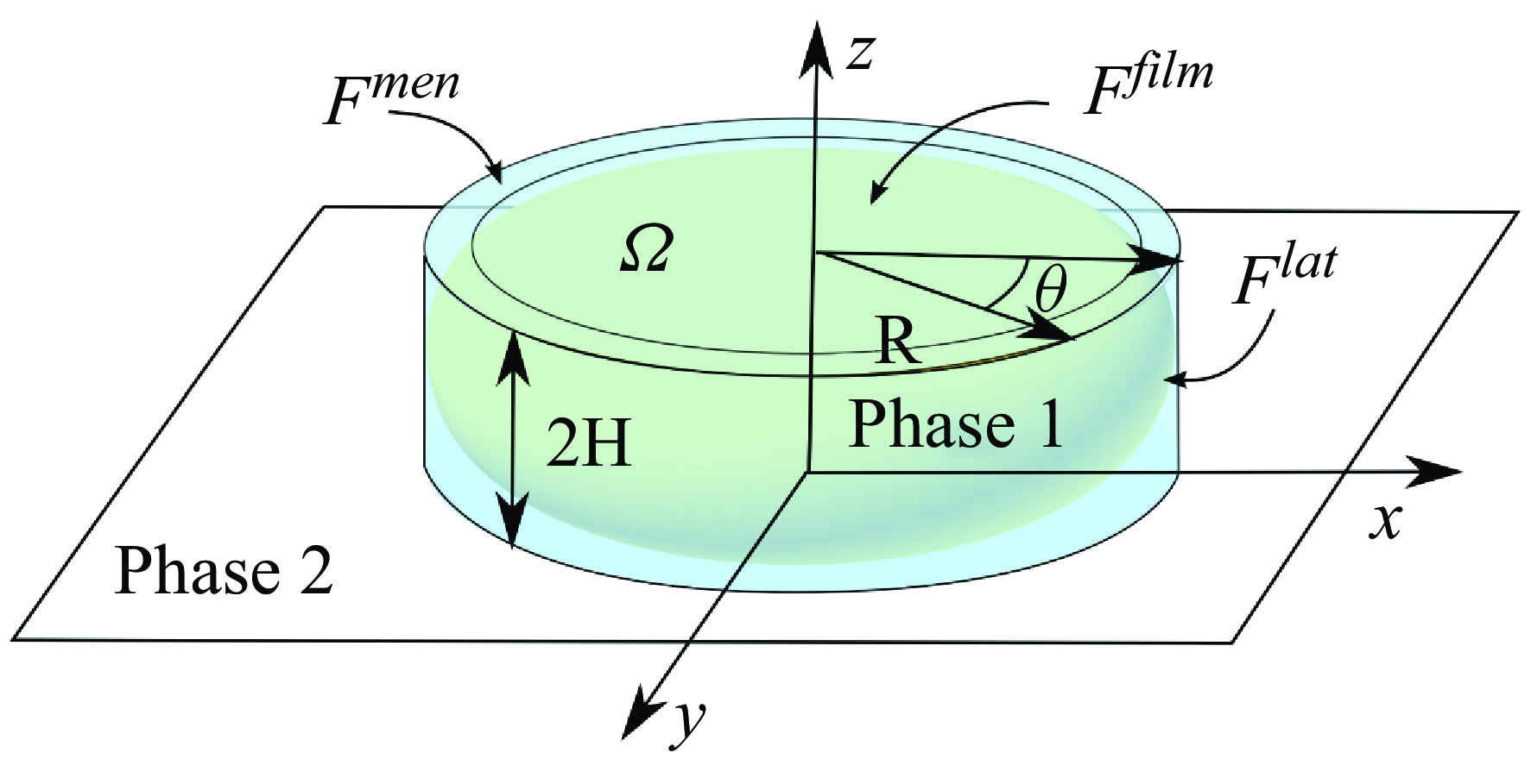
Schematic representation of the pancake droplet in the Hele-Shaw cell, and notations used in the text. The problem is solved in the laboratory frame, in which the droplet moves at velocity
 $U_d$
, pushed by the external phase,of velocity
 $U_\infty$
far from the droplet.

We first present an experimental investigation of the mobility of a pancake oil droplet pushed by an aqueous carrier phase in the presence of ionic surfactants. We investigated two surfactant families: alkyl ammonium bromides with 10, 12 or 14 carbons in the alkyl chain and the alkyl sulphates with 8, 10, 11 or 12 carbons. The experimental set-up is discussed in § 2 and the experimental results are presented in § 3. The main experimental result is that the droplet mobility increases with the droplet size for the most soluble surfactants (11 carbons or less for both families), whereas it decreases for the less soluble ones (12 carbons or more for both families). This second regime is in clear contradiction with the existing models of the literature. In § 4, we propose to model the droplet interface as a two-dimensional (2-D) incompressible liquid, which is the relevant limit for monolayers of poorly soluble surfactants (Mysels, Shinoda & Frankel Reference Mysels, Shinoda and Frankel1959; Seiwert, Dollet & Cantat Reference Seiwert, Dollet and Cantat2014). In this limit, the interface is able to produce a large Marangoni stress. The problem then involves three liquid phases: the droplet, the external phase and the interface, whose respective velocity fields are strongly coupled. Using analytical solutions built by Gallaire et al. (Reference Gallaire, Meliga, Laure and Baroud2014) for a cylindrical drop when the surface tension gradient is imposed (a decoupled problem), we solve the coupled problem and predict analytically the droplet mobility and the surface tension gradient without any adjustable parameter. This model quantitatively predicts the experimental mobility obtained for the less soluble surfactants and captures its variation with the droplet size and the capillary number. We thus believe that the variation of the droplet mobility with its size is an indication of the influence of the surface tension gradients induced by the droplet motion itself: in this regime, the droplet motion is limited by the surfactant flux from its rear to the front, on its lateral sides. Interestingly, our approach shows that when the incompressibility assumption is relaxed and the interface is considered stressfree, it is possible to derive a maximum mobility for the more soluble surfactants, in agreement with the experimental data. Our analytical approach can therefore predict the droplet velocity for poorly soluble surfactants. For more soluble surfactants, the droplet velocity is bounded between the two limits of stress-free interface and incompressible interface, respectively.
2. Experimental methods
2.1. Experimental set-up
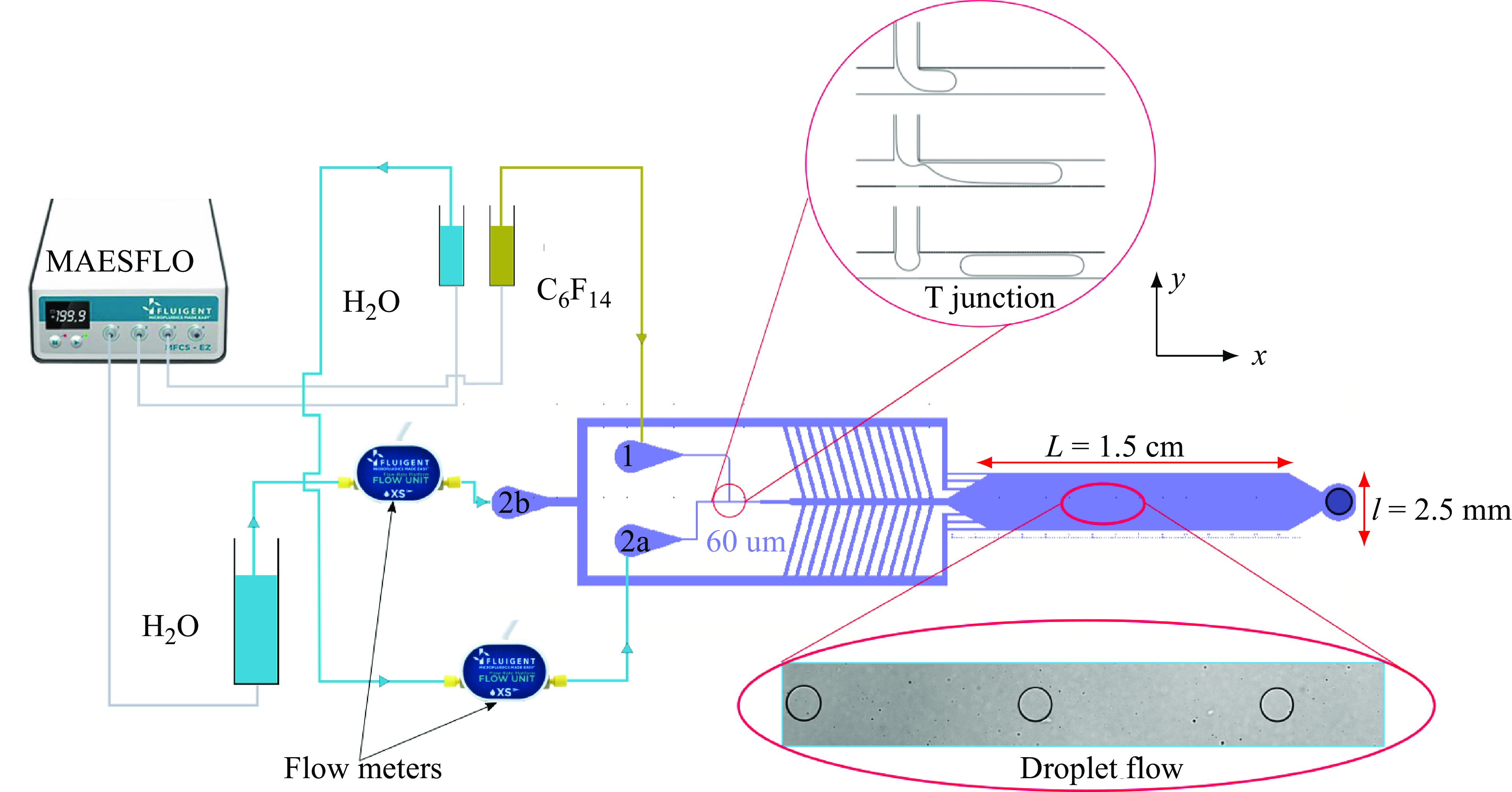
Design of the experimental set-up. The PDMS chip is shown in purple, with an enlarged schematic picture of the T-junction (top red circle) used to produce the droplets, and an experimental picture of the droplets in the Hele-Shaw cell (bottom red ellipse). The three pressure controllers and two flowmeter are shown on the left.

The microfluidic chips are manufactured in polydimethylsiloxane (PDMS) using standard soft lithography (Xia & Whitesides Reference Xia and Whitesides1998). Sylgard 184, bought from NEYCO company, is mixed with a curing agent at a 1:10 ratio and placed in a vacuum desiccator for half an hour. The mixture is then poured on a mould, fabricated using a photolithography SU8 photoresist layer and put in an oven at 70 °C for 2 hours. The resulting PDMS microfluidic chip is then permanently bonded to a glass slide via oxygen plasma. The glass slide has been previously cleaned of any dust and biological contamination by being immersed in a Piranha solution with a ratio of 1/3 hydrogen peroxyde (H
 $_2$
O
 $_2$
50 %) and 2/3 of sulphuric acid (H
 $_2$
SO
 $_4$
) for 5 minutes, rinsed with milli-Q water and dried using compressed air.
The oil droplets are generated at the T-junction shown in the inset of figure 2. The internal phase (phase 1) is fluorinated-oil FC72 (C
 $_6$
F
 $_{14}$
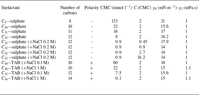
, Sigma Aldrich) and is injected in inlet (1) while an aqueous phase (phase 2) is injected in inlets (2a) and (2b). The various surfactant solutions used for this external phase are listed in table 1. The viscosity of the two solutions are
 $\eta _1=0.3$
mPa.s and
 $\eta _2$
which varies from 1–1.5 mPa.s, leading to a viscosity ratio
 $\eta _1/\eta _2\sim 0.3$
down to 0.2.
Properties of the aqueous solutions depending on the surfactants used in the preparation. All the data have been determined using the pendant-drop method for the interface properties and Couetter heology for the viscosity.

Experiments are performed with several microfluidic chips with microchannels at inlets (1) and (2a) of width between 60
 $\unicode{x03BC}$
m and 150
 $\unicode{x03BC}$
m. As such, it is possible to vary the radius of the generated droplets from
 $45$
to
 $130$
 $\unicode{x03BC}$
m by adjusting both the imposed pressures at inlets (1) and (2a) and the microchannel widths. The external flow rate is independently controlled using the second inlet of aqueous solution (2b). This additional aqueous solution is progressively injected in the main channel through a comb of lateral channels to avoid droplet breakup that would otherwise occur at high flux with a single lateral channel.
The pressures at the 3 inlets are controlled by a MAESFLO pressure controller, and the aqueous flow rates
 $Q_{2a}$
and
 $Q_{2b}$
, respectively, at inlets (2a) and (2b) are measured with a Fluigent flowmeter. The total flow rate of phase 2 is in the range [1–100]
 $\unicode{x03BC}$
l min–1 and the flow rate of phase 1 is of the order of a few
 $\unicode{x03BC}$
l min–1. The pressure at the inlets are in the range [50–500] mBar, so the actual pressure in the Hele-Shaw cell is below this value.
The droplets eventually reach the Hele-Shaw cell of height
 $2H = 15\ \unicode{x03BC} \rm m$
, length
 $L = 1.5$
cm in the direction of the flow (the
 $x$
direction, as shown in figure 2 ) and width
 $l = 2.5$
mm in the transverse direction (the
 $y$
direction). The outlet of the Hele-Shaw cell is directly connected to the atmospheric pressure, to minimise the average pressure in the cavity and thus avoid deformations of the PDMS chip. This was checked by measuring the shape of the cavity using a fluorescein absorbance method (Huerre et al. Reference Huerre, Theodoly, Leshansky, Valignat, Cantat and Jullien2015; Baué Reference Baué2022) and we found no deformations by the flow, even at the highest flow rates. The room temperature is kept constant at 20 °C. The average velocity of the external phase in the Hele-Shaw cell can therefore be computed as
 $U_\infty = (Q_{2a} + Q_{2b})/(2H \,l)$
, the oil flow rate being negligible.
2.2. Image recording and processing
The droplets are observed through a Leica DMIRB Microscope and recorded with a Zyla (Andor) camera with a sCMOS sensor connected to the microscope, at 50 frames per second, with a resolution of 1.3
 $\unicode{x03BC}$
m pixel–1. The droplets are separated by a distance larger than ten times their radius in order to avoid any hydrodynamic interactions between them (Shen et al. Reference Shen, Leman, Reyssat and Tabeling2014). There are typically 2 or 3 droplets in the video camera’s field of view. The droplet shape is determined by image processing. The diameters in the
 $x$
and
 $y$
directions differ by less than 3
 $\%$
, indicating a very good circularity. The droplet radius is determined as
 $R= \sqrt {A/\pi }$
, with
 $A$
corresponding to the droplet area. For each data series, the droplet radius is controlled with a precision of
 $\pm 5\ \unicode{x03BC}$
m.
Each droplet is followed along its trajectory by image correlation, and the instantaneous droplet velocity is computed. We first verify that the velocity varies by less than 5
 $\%$
along the whole trajectory, if the first and last millimetre of the Hele-Shaw cell are disregarded. Then trajectories are recorded within the observational window of length 3 mm near the centre of the cell, and the mean droplet velocity is measured along these trajectories. Each droplet velocity
 $U_d$
shown below has been obtained by averaging the velocity over 50 droplets. The dispersion of the data obtained on the different droplets provides the error bars. The highest measurable droplet velocity is of the order of
 $U_d = 2$
cm s–1, and is limited by the image acquisition rate.
2.3. Aqueous solution preparation
Two series of surfactants are used in the experiments: sodium alkyl sulphates, with an anionic head, noted C
 $_{n}$
-sulphate with
 $n = [8,10,11,12]$
being the number of carbons in the alkyl chain; and alkyl trimethylammonium bromides, with a cationic head, noted C
 $_n$
-TAB with
 $n = [10,12,14]$
. All surfactant provided by SigmaAldrich have a 99 % purity, except for the C
 $_{14}-$
TAB which is 95 % pure. They were dissolved in milli-Q water. The properties and concentration of the surfactant solutions used are listed in table 1. Due to the positive charge of the ammonium, the wetting film separating the oil droplet from the wall tends to rupture, especially at low velocity, as the glass substrate is charged negatively. In order to avoid the wetting of the droplets on the glass at low capillary numbers, salt is added in the solutions between 0.1 and 1 mol l–1 to decrease the Debye lengths and therefore lower the range of the electrostatic interactions. Moreover, the experiments with C
 $_n$
TAB surfactants needed to be started at high pressure to de-wet the oil from the microchannels. To understand how the addition of salt influences the interface properties, C
 $_{12}-$
sulphate experiments were carried out with and without the salt.
3. Experimental results
We first address the effect of the surfactant concentrations on the mobility of the droplet. To this end, we used C
 $_{12}-$
sulphate solutions of concentration in the range [
 $0.41$
–
 $16.4$
] mM with NaCl at concentration 0.2 M. The surfactant concentration was thus varied from 0.45 CMC (critical micellar concentration) up to 18.2 CMC, i.e. on either side of the CMC. The concentrations are expressed relatively to the CMC in table 1. Note that the CMC depends on the salt concentration, see column 4. The effect of salt was also investigated with the C
 $_{12}-$
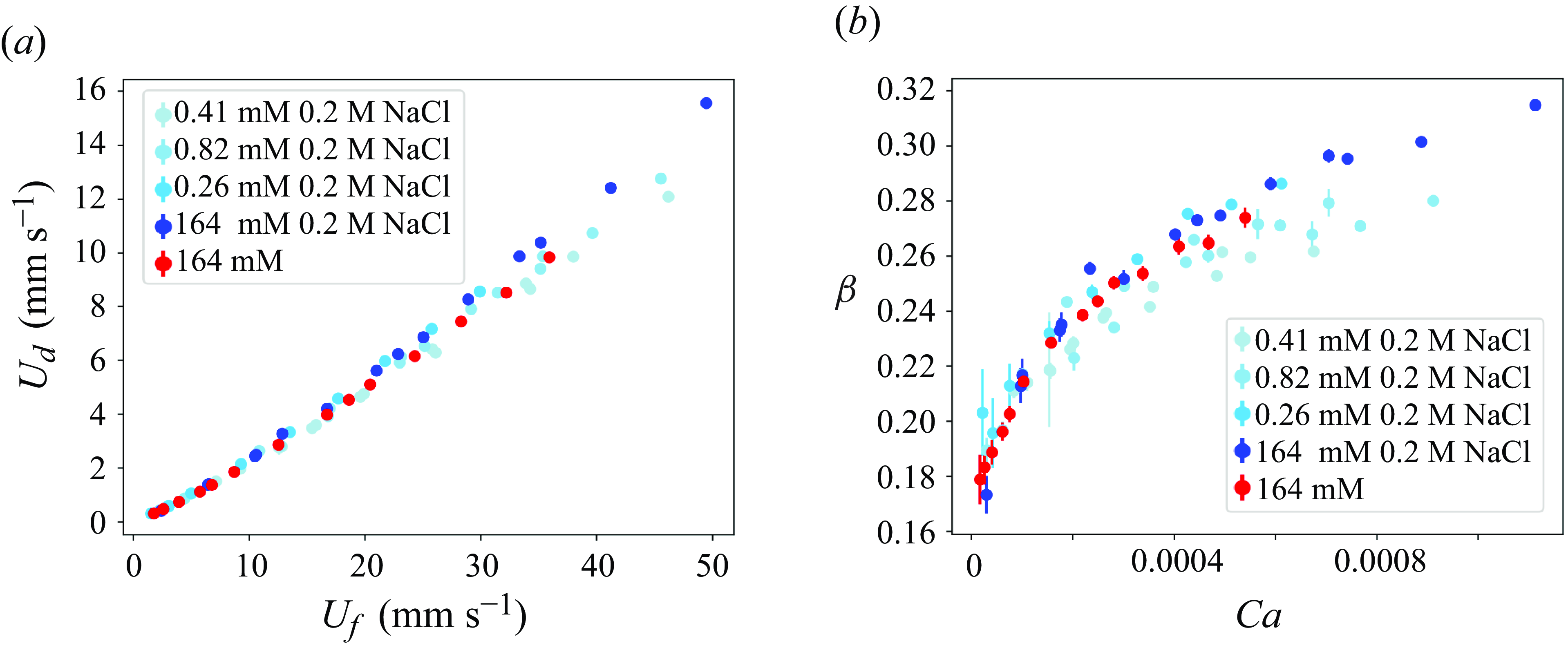
sulphate solution at the largest concentration, which was prepared without salt or with a concentration of 0.2 M NaCl. In figure 3(a) we plot the velocity of the droplet
 $U_d$
as a function of the velocity of the carrier phase
 $U_\infty$
for all these solutions, for a droplet radius
 $R= 90 \pm 5 \, \unicode{x03BC}$
m. The droplet velocity varies faster than linearly with
 $U_\infty$
, which is more visible in figure 3(b) where we plot the mobility
 $\beta = U_d/U_\infty$
as a function of
 $Ca = \eta _2 U_d / \gamma$
. No significant influence of the salt concentration has been observed for the investigated range of parameters. When the concentration of C
 $_{12}-$
sulphate increases, a slight increase of the droplet velocity is observed in figure 3(a). Some dispersion remains in figure 3(b), of the order of
 $3 \times 10^{-2}$
at
 $Ca = 5 \times 10^{-4}$
, but with a different trend: as
 $Ca$
is increased, the mobility seems to first increase and then decrease with the surfactant concentration.
Droplet velocity
 $U_d$
for different concentrations of C
 $_{12}-$
sulphate and of NaCl. (a) Value of
 $U_d$
as a function of the carrier phase velocity
 $U_\infty$
. (b) Mobility
 $\beta =U_d/U_\infty$
as a function of the capillary number
 $Ca= \eta _2 U_d/\gamma$
. The droplet radius is
 $R= 90 \pm 5 \, \unicode{x03BC}$
m.

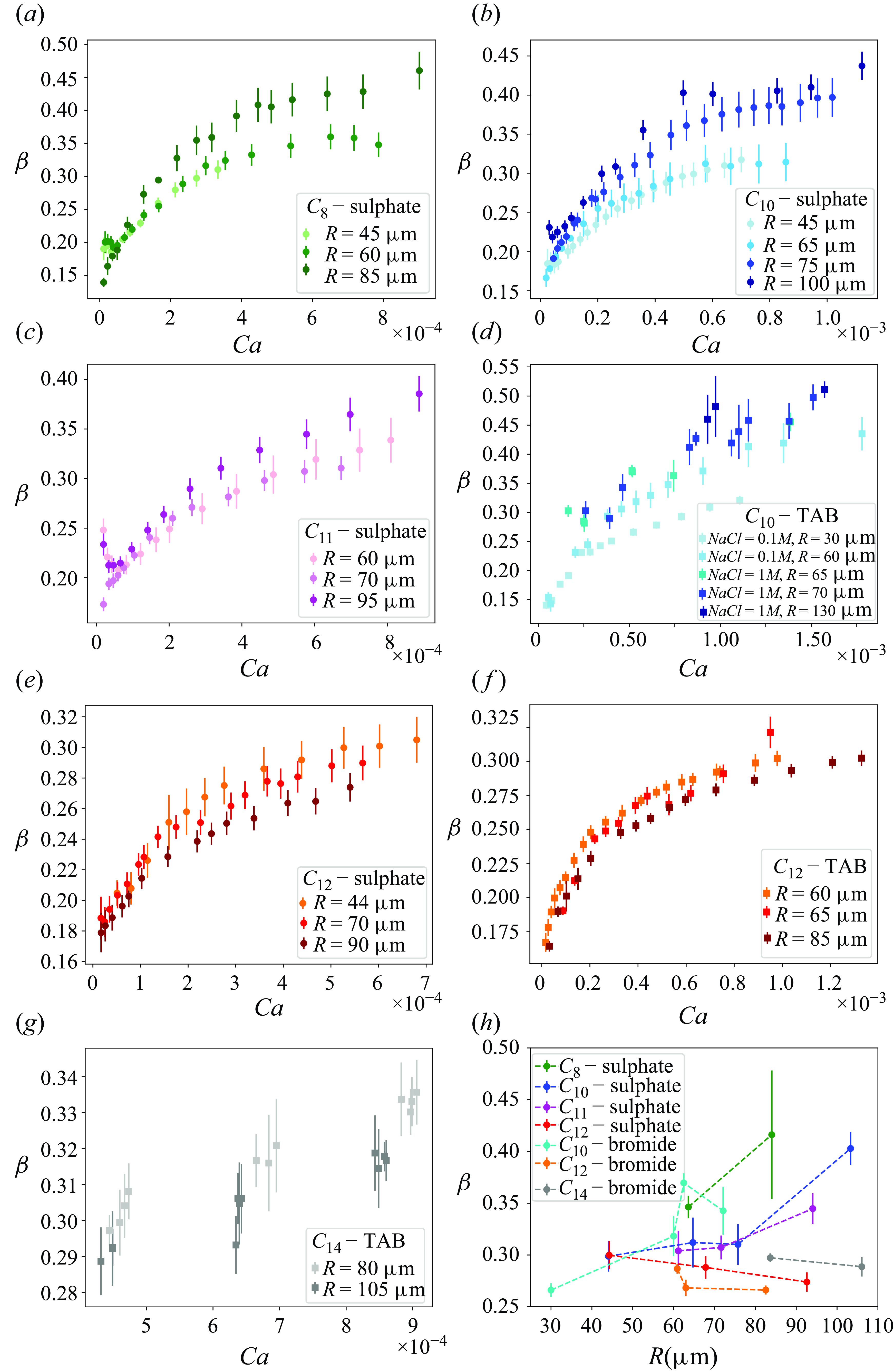
Mobility
 $\beta = U_d/U_\infty$
as a function of the capillary number for several radii for (a) C
 $_{8}-$
sulphate, (b) C
 $_{10}-$
sulphate, (c) C
 $_{11}-$
sulphate and (d) C
 $_{10}-$
TAB, (e) C
 $_{12}-$
sulphate, (f) C
 $_{12}-$
TAB, (g) C
 $_{14}-$
TAB. (h) Mobility of the droplets as a function of their radii for
 $Ca= 5 \times 10^{-4}$
.

In figure 4 we focus on the influence of the droplet size, for different surfactants. The C
 $_n$
-sulphate solutions are all prepared at 2 CMC, without salt, and the C
 $_n$
-TAB solutions at 2 CMC with salt at 0.1 M or 1 M, as specified in the figure legends (see table 1). For each solution, the mobility
 $\beta$
of the droplets is plotted for several droplets radii. The mobility of the droplets increases with the capillary number as already shown in figure 3, and depends on the droplet size.
In order to highlight this radius dependency, the data of figure 4(a–g) have been interpolated in the capillary number range [
 $10^{-4}$
–
 $10^{-3}$
] so that we get a mobility value for all the solutions at the same capillary number chosen at
 $Ca=5 \times 10^{-4}$
. The resulting mobilities are plotted in figure 4(h) as a function of the droplet radius. The variations with the droplet radius are small but clear trends are emerging, and the variation of the mobility with the nature of the surfactant is larger than the variation obtained by changing the salt or surfactant concentrations in figure 3(b). In the following, we thus focus on the variations of the mobility with the droplet radius, the capillary number and the nature of the surfactants and disregard the effect of the surfactant or salt concentrations. For the surfactants having a carbon chain with 11 carbons or less, in both surfactants families, we observe that the mobility increases with the droplet radius. This is the expected regime discussed in § 1. The central result of this paper is that, for the surfactants having a carbon chain with 12 carbons or more, the mobility of droplets in contrast decreases with the droplet radius. This observation confirms preliminary observations made in Reichert (Reference Reichert2017). This regime, observed for the longest carbon chains, is in contradiction with the existing models in the literature, but is quantitatively predicted by the model developed below.
4. Modelling
4.1. Main assumptions of the model
The control volume
 $\Omega$
is a cylinder of axis
 $Oz$
, in contact with the top and bottom walls, and of radius
 $R$
, so that its lateral side is just outside the drop, represented in yellow (through transparency). The external forces acting on
 $\Omega$
are decomposed into
 $\textbf {F}^{film}$
, acting on the top and bottom faces of the cylinder,
 $\textbf {F}^{lat}$
, acting on its side, and
 $\textbf {F}^{men}$
, localised at the top and bottom faces, in the dynamical meniscus.

In our experimental regime, the viscous stress remains smaller than the capillary forces so the drop can be assumed to remain circular, as shown in § 2.2. It is separated from the wall by a film of thickness
 $h$
that is assumed to be uniform, as discussed in § 4.5. The drop’s shape can thus be decomposed into a cylindrical part of radius
 $R-H \sim R \gg H$
and thickness
 $2(H-h) \sim 2H \gg h$
, bounded by a meniscus with a semi-circular section of radius
 $H-h \sim H$
(see figure 5).
Our model involves three main unknowns, the drop velocity
 $U_d$
, the interface velocity in the wetting film
 $U_s$
, assumed to be uniform as discussed in § 4.4, and the tension difference between the front and the rear of the drop
 $2 \Delta \gamma$
. These unknowns are coupled to each other through (i) the force balance on the drop, (ii) the interface area conservation, which expresses the surfactant conservation, and (iii) the consistency of the tension difference computed either along the drop side or along the wetting films. These three couplings allow us to predict the drop velocity as a function of the imposed velocity
 $U_\infty$
.
The force balance on the drop is thus made on the control volume
 $\Omega$
, shown in figure 5, which shape is known. It is a cylinder of axis
 $Oz$
, in contact with the top and bottom walls, and of radius
 $R$
, so that its lateral side is just outside the drop. The force
 $F^{lat}$
exerted on
 $\Omega$
is governed by the viscous flows inside and outside the drop. They are calculated in § 4.2 by identifying the shape of
 $\Omega$
and the shape of the drop. Indeed, for this part of the problem, we assume that the viscosities are equal to
 $\eta _1$
and
 $\eta _2$
, respectively, inside and outside
 $\Omega$
and that the surface tension acts on the lateral side of
 $\Omega$
and does not depend on
 $z$
. On the scale of the droplet, the interface velocity in the wetting film
 $U_s$
, assumed to be proportional to
 $U_d$
, plays the role of a sliding velocity for the drop. These simplifications neglect some viscous contributions in the meniscus domain, i.e. in the volume between the lateral side of
 $\Omega$
and the actual position of the drop interface. Therefore, this approach accounts for all physical effects (Nagel & Gallaire Reference Nagel and Gallaire2015), but cannot be considered as a rigorous
 $H/R$
expansion. However, the largest viscous forces in these volumes are actually localised close to the walls and are taken into account quantitatively in § 4.5, where
 $\textbf {F}^{men}$
is determined using the lubrication equations on the wetting film scale. Finally, the contribution
 $\textbf {F}^{film}$
of the wall in the wetting film domain is determined in § 4.4.
The key assumption of the model is the interface area conservation. Deformation of the interface (compression or extension) does not occur because it would lead to high surface tension variations. The interface behaves as a perfectly incompressible 2-D fluid and the surface tension is computed as the Lagrange multiplier associated with the incompressibility constraint. This corresponds to the limit of high Gibbs modulus, and is thus more likely to be reached for poorly soluble surfactants.
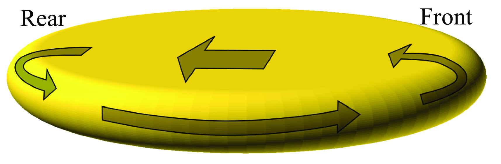
Schematic showing the velocity field on the drop interface, in the frame of the drop. In this frame, the top and bottom walls move to the left at the velocity
 $-U_d$
and the drop interface in the thin film moves almost at the same velocity (if
 $U_s \ll U_d$
), inducing a surfactant flux to the left which scales as
 $-R U_d$
. This tank-treading motion of an incompressible interface corresponds to the rolling case in Cantat (Reference Cantat2013). This flux must be balanced by a flux on the drop side.

The flow pattern obtained in the regime of incompressible interface is schematically anticipated in figure 6 for the simple case where the interface velocity
 $U_s$
remains much smaller than
 $U_d$
(rolling case in Cantat (Reference Cantat2013)). Then, in the frame of the drop, the pieces of interface covering the wetting films move at a velocity of the order of
 $-U_d$
, inducing an interface flux to the rear of the drop which scales as
 $- U_d R$
. The constraint of interface incompressibility imposes that this flux is balanced by a flux toward the front, which occurs on the lateral sides of the drop, as proposed in Park, Maruvada & Yoon (Reference Park, Maruvada and Yoon1994) and observed in Lee, Gallaire & Baroud (Reference Lee, Gallaire and Baroud2012). In this region, the velocity scales as
 $U_\infty$
(as
 $U_\infty \gg U_d$
), the flux as
 $U_\infty H$
and the flux balance thus leads to
 $U_d \sim U_\infty H/R$
. This qualitative scaling law identifies the origin of the decrease in droplet velocity as a function of droplet size. However, it does not account for the observed dependence on
 $Ca$
. The quantitative model developed below will show that the coupled dependencies on
 $R$
and
 $Ca$
of droplet mobility do not follow a scaling law, and result instead from a complex balance between different terms.
Note that the assumption of negligible surface tension difference between the front and the rear of the drop used in Dangla (Reference Dangla2012) corresponds to the opposite limit: any extension or compression of the interface induces sufficiently fast surfactant adsorption or desorption to avoid surface tension variations, which is expected to be valid for high surfactant solubility.
4.2. Solutions of Brinkman’s equation for a circular profile
Firstly, we determine the expression for the velocity field inside and outside the drop as a function of
 $U_\infty$
and of the unknowns
 $U_d$
,
 $U_s$
and
 $\Delta \gamma$
. The Hele-Shaw equation is usually used in our geometry to model the flow. However, it entirely neglects viscous effects due to in-plane velocity gradients, which implies that tangential velocities are not prescribed at the drop interface and may be discontinuous. This precludes any coupling between the surfactant motion at the drop interface and the external velocity field, which is the main physical process governing the drop motion. The coupling is accounted for using Brinkman’s equation (Nadim, Borhan & Haj-Hariri Reference Nadim, Borhan and Haj-Hariri1996; Boos & Thess Reference Boos and Thess1997; Bush Reference Bush1997; Gallaire et al. Reference Gallaire, Meliga, Laure and Baroud2014). As already mentioned, here, we assume that the droplet is cylindrical. The effects of the meniscus and of the thin film are taken into account in §§ 4.4 and 4.5.
The Stokes equations in each phase
 $i$
are
 \begin{equation} \eta _i \left (\frac {\partial ^2 \textbf {u}_i}{\partial z^2} + \Delta _{2D} \textbf {u}_i \right ) = \nabla p_i \quad \text{and} \quad \mbox {div}\, \textbf {u}_i =0 \; , \end{equation}
where
 $\textbf {u}_i$
is the velocity of the phase
 $i$
in the laboratory frame and
 $p_i$
is its pressure. The indices
 $i=1$
and
 $i=2$
indicate the internal and external phases, respectively. For the external phase, the velocity vanishes at
 $y=0$
and
 $y=2 H$
. Brinkman’s assumption is that the velocity field remains parabolic as for the classical Hele-Shaw problem. We therefore have
 \begin{equation} \textbf {u}_2 = \textbf {U}_2 \, \frac {3 z(2H-z)}{2 H^2} \;, \end{equation}
where
 $ \textbf {U}_2(x,y)$
is the depth-averaged velocity in the phase 2 and
 \begin{equation} \eta _2 \left ( \Delta _{2D} \textbf {U}_2 - \frac {3}{H^2} \textbf {U}_2 \right ) = \nabla p_2 \, . \end{equation}
The phase 1, in the drop, obeys similar equations. However, the top and bottom boundary conditions differ from the ones used for the external phase. The drop is separated from the wall by a thin layer of the external phase of thickness
 $h$
, and the oil/water interfaces, at the positions
 $h$
and
 $2H-h$
, respectively, move at the velocity
 $ \textbf {U}_s$
. We assume that
 $\textbf {U}_s= \unicode{x03BC} \textbf {U}_d$
, where
 $\unicode{x03BC}$
is a constant, and that
 $h$
is uniform in the wetting film. Brinkman’s solution of (4.1) is slightly modified to take into account this specific constraint
 \begin{equation} \textbf {u}_1 = (\textbf {U}_1 - \textbf {U}_s)\, \frac {3 (z-h)(2H-h-z)}{2 (H-h)^2} + \textbf {U}_s\;, \end{equation}
where
 $ \textbf {U}_1(x,y)$
is the depth-averaged velocity in the phase 1 and
 \begin{equation} \eta _1 \left ( \Delta _{2D} \textbf {U}_1 - \frac {3}{(H-h)^2} (\textbf {U}_1 - \textbf {U}_s) \right )= \nabla p_1 \, . \end{equation}
Following Gallaire et al. (Reference Gallaire, Meliga, Laure and Baroud2014), we define in each phase a streamfunction
 $\Psi _i(r,\theta )$
, with the origin of the polar coordinates
 $(r,\theta )$
at the centre of the circular drop and
 $\theta =0$
in the direction of motion
 $\textbf {e}_x$
(see figure 7
a). The velocity field is
 $\textbf {U}_i=(U_{r,i}, U_{\theta ,i})$
, with
 $U_{r,i} = (1/r) \partial _\theta \Psi _i$
and
 $U_{\theta ,i} = - \partial _r \Psi _i$
.
The equations of motion (4.3) and (4.5) can be expressed as
 \begin{equation} \Delta _{2D} \left (\Delta _{2D} - \frac {k^2}{R^2} \right ) \Psi _i = 0 \, , \end{equation}
with
 $k= \sqrt {3} R/H$
. For the internal phase, we use the assumption that
 $\textbf {U}_s$
is uniform and that
 $h\ll H$
.
The fluid motion in both phases is driven by the boundary conditions. At the drop lateral boundary, the average normal velocity is
 $U_{r,i}(R, \theta )= U_d \cos \theta$
in both phases and the tangential velocity is continuous so
 $U_{\theta ,2}(R, \theta )=U_{\theta ,1}(R, \theta )$
. At large
 $r$
, the velocity is
 $\mathbf {U_2}= U_\infty \textbf {e}_x$
. Finally, the tangential stress continuity imposes that
 \begin{equation} \eta _1 \left ( r \partial _r \left (\frac {U_{\theta ,1}}{r}\right )+ \frac {1}{r} \partial _\theta U_{r,1}\right ) - \eta _2 \left ( r \partial _r \left ( \frac {U_{\theta ,2}}{r} \right ) + \frac {1}{r} \partial _\theta U_{r,2}\right ) = \frac {1}{r}\partial _\theta \gamma \; , \end{equation}
where
 $\gamma$
is the surface tension, averaged over the cell thickness, on the side of the drop. From the symmetry of the problem, we assume that
 $\gamma (\theta ) = \gamma _0 + \Delta \gamma \, x/R = \gamma _0 + \Delta \gamma \cos \theta$
.
The general solutions of (4.6) for these boundary conditions are established in Gallaire et al. (Reference Gallaire, Meliga, Laure and Baroud2014), where
 $U_d$
,
 $U_\infty$
and
 $\Delta \gamma$
are considered as external control parameters independent of each other. The solutions are of the form
 \begin{align} \Psi _1(r) & = \left ( a \frac {I_1(kr/R)}{I_1(k)} + b \frac {r}{R} \right ) \sin \theta \, , \nonumber \\ \Psi _2(r) & = \left (c \frac {K_1(kr/R)}{K_1(k)} + d \frac {R}{r} + e \frac {r}{R} \right ) \sin \theta \, , \end{align}
where
 $I_1$
and
 $K_1$
are the modified Bessel functions and
 $a$
,
 $b$
,
 $c$
,
 $d$
and
 $e$
are five constants determined by Gallaire et al. (Reference Gallaire, Meliga, Laure and Baroud2014) and given in Appendix A as a function of our unknown quantities
 $U_d$
,
 $U_\infty$
and
 $\Delta \gamma$
. The whole velocity field is thus known as a function of the parameters
 $U_d$
,
 $U_\infty$
,
 $\Delta \gamma$
and
 $U_s$
and can be used to express the three couplings that relate these parameters to each other.
Note that the Hele-Shaw equation, in which the Laplacian term is removed from (4.1), has solutions of the form (4.8) with
 $a=c=0$
,
 $b= RU_d$
,
 $d=R(U_d-U_\infty )$
and
 $e= R U_\infty$
. In that case, the velocity field in the drop is simply a uniform velocity
 $U_d \, \textbf {e}_x$
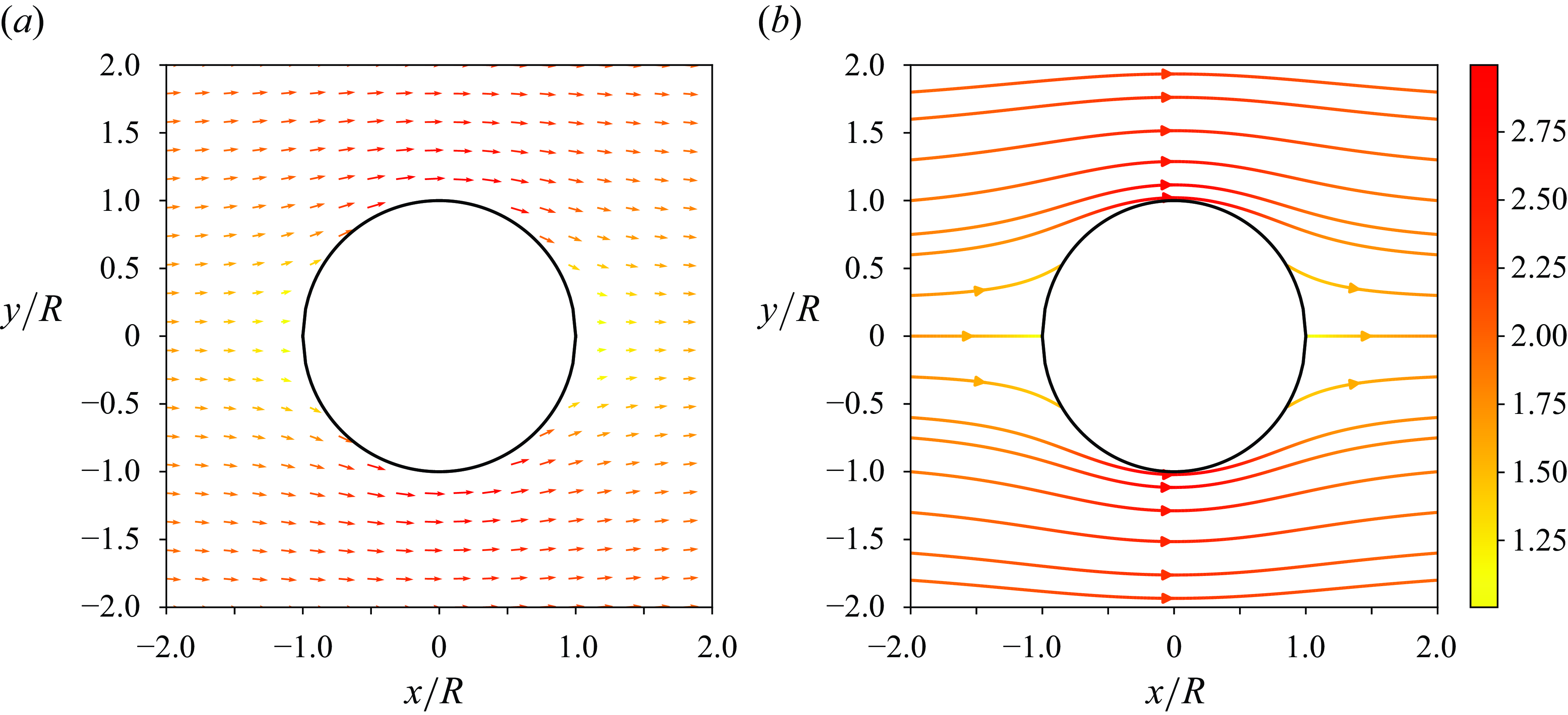
and the velocity field outside the droplet is shown in figure 7. This solution does not satisfy the continuity of the tangential velocity at the lateral interface, which can only be achieved with the additional Bessel functions. However this simpler solution is close to the actual solution and the Bessel function terms are non-negligible only close to the droplet lateral boundary, for
 $r$
in the range
 $[R-H , R+H]$
.
Flow around a drop moving in the
 $x$
direction, in the laboratory frame. (a) Velocity field around the droplet computed from (4.8) using
 $e= R U_\infty$
,
 $d=R(U_d-U_\infty )$
and
 $c=0$
, for the case
 $U_d=1$
and
 $U_\infty =2$
. (b) Streamlines around the droplet for the same parameters. The colour code indicates the value of
 $U_{2,x}/U_d$
.

4.3. Force on the drop side
From the velocity field obtained in § 4.2, and the results of (44), (55) and (63) in Gallaire et al. (Reference Gallaire, Meliga, Laure and Baroud2014), we can derive the force
 $F^{lat} \textbf {e}_x$
exerted by the external fluid on the lateral side of
 $\Omega$
(due to the pressure and viscous stresses)
 \begin{equation} F^{lat} = 12 \pi \eta _2 U_\infty \frac {R^2}{H} - 6 \pi \eta _2 U_d \frac {R^2}{H} - 4 \pi \Delta \gamma H \frac {\eta _2}{\eta _1+\eta _2} \, . \end{equation}
Note that the interface sliding velocity
 $U_s$
is zero in Gallaire et al. (Reference Gallaire, Meliga, Laure and Baroud2014) so the internal pressure
 $p_1$
, given by (4.5), is not the same in our case. However, this pressure is not used to compute
 $F^{lat}$
, so the results of Gallaire et al. (Reference Gallaire, Meliga, Laure and Baroud2014) directly apply in our case as well, even for
 $U_s$
of the order
 $U_d$
. By contrast, the friction on the top and bottom walls
 $F^{film}$
determined below does depend on the sliding velocity.
4.4. Contribution of the wetting film
The wetting film thickness
 $h$
is much smaller than the cell thickness
 $2H$
and the velocity in the wetting film thus corresponds to the velocity of a simple shear flow. In the bottom film
 \begin{equation} \textbf {u}^{film}(x,y,z) = \frac {z}{h} \textbf {U}_s(x,y) \; . \end{equation}
The tangential stress continuity in the flat film imposes a relationship between the tension and the velocity gradients along
 $z$
 \begin{equation} \eta _2 \frac {\textbf {U}_s}{h} - 3 \eta _1 \frac {(\textbf {U}_1 - \textbf {U}_s)}{H} = \nabla \gamma ^{film} \; , \end{equation}
where
 $\gamma ^{film}(x,y)$
is the tension in the bottom wetting film (or, by symmetry, in the top one).
In the central part of the droplet, i.e. at a distance at least
 $H$
from the drop boundary, the depth average velocity field
 $\textbf {U}_1$
is
 $U_d\,\bf {e}_x$
(see (4.8)). For sake of simplicity,
 $\textbf {U}_s$
is determined by assuming that this remains true in the whole film. Similarly, the surface tension gradient on the drop lateral side is uniform and oriented along
 $x$
and we assume that this remains true in the wetting film. Equation (4.11) thus implies that
 $\textbf {U}_s = U_s \textbf {e}_x$
, where
 $U_s$
is a constant.
We thus get
 \begin{equation} \eta _2 \frac {U_s}{h} - 3 \eta _1 \frac {(U_d - U_s)}{H} = \frac {\Delta \gamma ^{film}}{R} \; , \end{equation}
with
 $\Delta \gamma ^{film}$
the surface tension difference between the front of the drop and the drop centre, in the wetting film, and
 $\Delta \gamma ^{film}/R\, \textbf {e}_x$
the uniform tension gradient in the wetting film.
Schematics of the bottom of the drop in the
 $(x,z)$
plane, with
 $\Delta \gamma ^{film}$
defined.

As shown in figure 8,
 $\Delta \gamma ^{film}$
slightly differs from the quantity
 $\Delta \gamma$
introduced before as the surface tension varies across the dynamical meniscus, where the Poiseuille flow contribution becomes non-negligible. This will be discussed in § 4.5.
Finally, the force exerted by the wall on the top and bottom boundaries of
 $\Omega$
is simply due to the shear flow in both films
 \begin{equation} F^{film} = - \pi R^2 \frac {\eta _2}{h} U_s \times 2 \; . \end{equation}
4.5. Contribution of the meniscus motion
The surface tension difference between the front and the rear of a bubble in the same geometry is given in Cantat (Reference Cantat2013) as a function of the interface velocity, in the limit of incompressible interface. This surface tension difference is the sum of a term proportional to the drop size, due to the simple shear in the film, and a second term, independent of the drop size, due to the flows in the meniscus. The contribution of the simple shear in the film is already taken into account in (4.12) and we will only consider the meniscus contribution here, i.e. for the front meniscus, the difference between the meniscus tension
 $\gamma (R,0)$
and the tension at the front of the thin film
 $\gamma ^{film}(R,0)$
(see figure 8). This term comes from the fact that the interface at the front of the drop moves towards the wall (if
 $U_s \lt U_d$
), and thus expels the external phase out of the meniscus. This flow exerts some viscous friction on the interface, which reacts via a surface tension gradient: the tension is thus larger in the film than in the meniscus.
The tension difference obtained for a bubble can be used here, as it does not depend on the internal viscosity as long as
 $\eta _1/\eta _2 Ca^{1/3} \ll 1$
(Park & Homsy Reference Park and Homsy1984), which is verified in our case.
So, from (22) in Cantat (Reference Cantat2013)
 \begin{equation} \gamma ^{film}(R,0) - \gamma (R,0) = \gamma _0(3 \alpha Ca)^{2/3} \left (\frac {1.85}{2} - 1.27 \frac {U_s}{3 \alpha U_d} \right )\; , \end{equation}
with
 $ \alpha = 4 - 2 (U_s/U_d)$
.
Similarly, at the rear
 \begin{equation} \gamma ^{film}(R,\pi ) - \gamma (R,\pi ) = \gamma _0(3 \alpha Ca)^{2/3} \left (- \frac {0.53}{2} + 4 \frac {U_s}{3 \alpha U_d} \right ) \; . \end{equation}
In both equations, the first term is the contribution of the Poiseuille flow localised in the dynamical meniscus, which connects the flat film to the static meniscus of curvature
 $\sim 1/H$
, while the second term corresponds to the simple shear induced by
 $U_s$
in the same domain.
The external tension difference
 $ \Delta \gamma = (\gamma (R,0) - \gamma (R,\pi ) )/2$
, coupled to the external velocity field through (4.9), is finally
 \begin{equation} \Delta \gamma = \Delta \gamma ^{\textit{film}} + \frac {1}{2} \left (\gamma ^{\textit{film}}(R,\pi ) - \gamma (R,\pi ) - (\gamma ^{\textit{film}}(R,0) - \gamma (R,0) )\right ) \; . \end{equation}
The terms proportional to
 $U_s$
are neglected in (4.14) and (4.15) as higher-order corrections (since they are also multiplied by
 $Ca^{2/3}$
) and we assume
 $\alpha = 4$
corresponding to the tank-treading motion of an incompressible interface shown in figure 6 and denoted as the rolling case in Cantat (Reference Cantat2013). By matching the surface tension difference along the film and along the lateral meniscus, i.e. from (4.12), (4.14) and (4.15), we get the coupling (iii)
 \begin{equation} \Delta \gamma = \eta _2 U_s \frac {R}{h} - 3 \eta _1 (U_d - U_s) \frac {R}{H} - \frac {\xi }{2} \gamma _0(3\alpha Ca)^{2/3} \, , \end{equation}
with
 $\xi = (1.85+0.53)/2= 1.19$
.
The wetting film thickness is predicted by the same approach and is
 \begin{equation} h= \zeta H (3\alpha Ca)^{2/3} \, , \end{equation}
with
 $\zeta = 0.634$
. As the meniscus normal velocity varies with
 $\theta$
, the wetting film is slightly thinner at large
 $|y|$
(Reichert et al. Reference Reichert, Huerre, Theodoly, Valignat, Cantat and Jullien2018). This effect is not taken into account here. Equation (4.17) thus provides a coupling between our unknown quantities
 $U_d$
,
 $U_s$
and
 $\Delta \gamma$
.
Following (13) in Cantat (Reference Cantat2013), we get the force exerted by the wall on the top and bottom boundaries of
 $\Omega$
, along the top and bottom menisci
 \begin{equation} F^{men} = - \xi \gamma _0(3\alpha Ca)^{2/3} \times 2R \times 2 \, , \end{equation}
where the factor
 $2R$
comes from the front (or rear) meniscus length (projected on the
 $x=0$
line), and the factor 2 from the top and bottom menisci.
4.6. Force and flux balances
The force balance in the domain
 $\Omega$
around the drop is
 $F^{lat} + F^{men}+ F^{film}=0$
, so from (4.9), (4.13), (4.19), the coupling (i) becomes
 \begin{equation} 0 = 12 \pi \eta _2 U_\infty \frac {R^2}{H} - 6 \pi \eta _2 U_d \frac {R^2}{H} - 4 \pi \Delta \gamma H \frac {\eta _2}{\eta _1+\eta _2} - 4 \xi R \gamma _0 (3\alpha Ca)^{2/3} - 2 \pi \eta _2 U_s \frac { R^2 }{h} \, . \end{equation}
Finally, the coupling (ii) between the sliding velocity
 $U_s$
and the drop velocity
 $U_d$
is given by the interface conservation. In the drop frame, the interface flux across the plane
 $x=0$
is zero due to the assumption of interface incompressibility. The lateral velocity in the laboratory frame is
 $\textbf {u}^{lat} = - u_\theta (R, \pi /2) \textbf {e}_x$
. It is computed from the velocity field in Appendix B and we get
 \begin{equation} u^{lat} = \frac {2 \eta _2}{\eta _1 + \eta _2} (U_\infty - U_d) + U_d+ \frac {\Delta \gamma }{\eta _1+ \eta _2} \frac {H}{\sqrt {3}R} \, , \end{equation}
so the lateral flux in the drop frame is
 \begin{equation} \Phi ^{lat} = 4 H \left ( \frac {2 \eta_2}{\eta _1 + \eta _2} (U_\infty - U_d) + \frac {\Delta \gamma }{\eta _1+ \eta _2} \frac {H}{\sqrt {3}R} \right )\,. \end{equation}
Note that this flux assumes that the meniscus side is a simple cylinder, with a section in the plane
 $x=0$
of length
 $2H$
and that the velocity does not depend on
 $z$
. This simple calculation is consistent with the use of the depth average velocities in our model. Note that integrating the velocity field (4.2) along the actual semi-circular shape of the meniscus leads to an additional prefactor
 $3 \pi /8 \sim 1.17$
in (4.22).
The flux in the two wetting films in the drop frame is
 \begin{equation} \Phi ^{film} = 4 R (U_s-U_d)\, , \end{equation}
leading to the conservation condition
 \begin{equation} \frac {2 \eta _2}{\eta _1 + \eta _2} (U_\infty - U_d) + \frac {\Delta \gamma }{\eta _1+ \eta _2} \frac {H}{\sqrt {3}R} + \frac {R}{H} (U_s-U_d) = 0\, . \end{equation}
5. Resolution of the equation set and comparison with the experiments
The tension consistency, (4.17), the force balance on the drop, (4.20), and the surfactant conservation, (4.24), can be rewritten as
 \begin{align} & \frac {U_s}{U_\infty } \left (\frac {R}{\zeta H} (3\alpha Ca)^{-2/3} + 3 \frac {\eta _1}{\eta _2} \frac {R}{H} \right ) -\frac {\Delta \gamma }{\eta _2 U_\infty } - \frac {U_d}{U_\infty } \left ( 3 \frac {\eta _1}{\eta _2} \frac {R}{H} + \frac {3 \alpha }{2} \xi (3\alpha Ca)^{-1/3} \right ) =0 \; , \end{align}
 \begin{align} & \frac {U_s}{U_\infty } \frac { 1 }{\zeta } (3\alpha Ca)^{-2/3} + \frac {\Delta \gamma }{\eta _2 U_\infty } \frac {2 \eta _2}{\eta _1+\eta _2} \frac {H^2}{R^2} + \frac {U_d}{U_\infty } \left ( 3 + \frac {6 \alpha \xi }{\pi } \frac {H}{R} (3\alpha Ca)^{-1/3} \right ) = 6 \; ,\\[-4pt]\nonumber \end{align}
 \begin{align} & \frac {U_s}{U_\infty } \frac {R}{H} + \frac {\Delta \gamma }{\eta _2 U_\infty } \frac {\eta _2}{\eta _1+ \eta _2} \frac {H}{\sqrt {3}R} - \frac {U_d}{U_\infty } \left ( \frac {R}{H} + \frac {2 \eta _2}{\eta _1 + \eta _2} \right ) = - \frac {2 \eta _2}{\eta _1 + \eta _2} \; . \end{align}
This constitutes a set of three linear equations with
 $U_d/U_\infty$
,
 $U_s/U_\infty$
and
 $\Delta \gamma /(\eta _2 U_\infty )$
as unknown parameters. Note that
 $U_d$
also implicitly appears in
 $Ca= \eta _2 U_d/\gamma$
. The problem is solved by considering
 $Ca$
as an independent parameter: this leads to the exact solution of the system, but in the form of an implicit expression.
5.1. First-order solution
The problem is first solved in a simplified form by assuming that
 $\beta = U_d/U_\infty$
,
 $H/R$
and
 $Ca^{1/3}$
are small parameters of the same order
 $\varepsilon \sim 0.1$
, as observed experimentally. The consistency of the system (5.1)–(5.3) imposes, under these assumptions, that
 $U_s/U_\infty$
is of order 2 and
 $\Delta \gamma /(\eta _2 U_\infty )$
of order
 $-1$
. The small value expected for
 $U_s$
is consistent with the value
 $\alpha =4$
chosen for this parameter in § 4.5, and kept in the following. At the leading order, the equation set is then given by
 \begin{equation} \begin{cases} \dfrac {U_s}{U_\infty } \, \dfrac {R}{\zeta H} (12 Ca)^{-2/3} - \dfrac {\Delta \gamma }{\eta _2 U_\infty } =0 \; , \\[12pt] \dfrac {U_s}{U_\infty } \dfrac {1 }{\zeta } (12 Ca)^{-2/3} = 6 \; , \\[12pt] \dfrac {\Delta \gamma }{\eta _2 U_\infty } \dfrac {\eta _2}{\eta _1+ \eta _2} \dfrac {H}{\sqrt {3}R} - \dfrac {U_d}{U_\infty } \dfrac {R}{H} = - \dfrac {2 \eta _2}{\eta _1 + \eta _2} \; , \end{cases} \end{equation}
leading to the leading-order solution
 \begin{align} & \Delta \gamma ^0 = 6 \eta _2 \frac {R}{H} \, U_\infty \, ,\\[-7pt]\nonumber \end{align}
 \begin{align} & U_s^0 = 6 \zeta (12 Ca)^{2/3}\, U_\infty \, , \\[-7pt]\nonumber\end{align}
 \begin{align} & U_d^0 = U_\infty \frac { 2 (1+ \sqrt {3})\, \eta _2}{\eta _1+\eta _2} \frac {H}{R} \, . \end{align}
This first-order solution reveals the dominant couplings. The tension difference verifies
 $\Delta \gamma \sim \Delta \gamma _{\textit{film}}$
and can be deduced from the consistency of the pressure field. The pressure drop between the rear and the front of the drop can first be calculated in the external flow field. As the drop is almost static, the parameters (A3) determine the flow, and (4.3) then leads to
 $\Delta p = 12 \eta _2 U_\infty \, R/H^2$
. This pressure drop can also be calculated across the droplet: in the limit of small droplet velocity, it is only due to the Laplace pressure jumps at the rear and at the front, so
 $\Delta p = 2 \Delta \gamma /H$
. Equating both expressions leads to the result (5.5). The order of magnitude we obtain for
 $U_\infty = 30$
mm s–1 is
 $\Delta \gamma \sim 2$
mN m–1, which is easily reached for interfaces in out of equilibrium conditions. This surface tension variation is a key difference between this model and previous approaches in which the tension variations are either absent, or related to the meniscus motion via the scaling
 $\gamma Ca^{2/3}$
.
The sliding velocity given by (5.6) can be obtained from the stress balance in the wetting film. Neglecting the viscous stress in the drop, the tangential stress continuity imposes
 $\Delta \gamma /R= \eta _2 U_s/h$
, with
 $h= \zeta H (12 Ca)^{2/3}$
. Here,
 $U_s$
is of the order of a few mm s–1.
Finally, the droplet velocity (5.7) is obtained from the surfactant flux balance. Neglecting
 $U_s$
, the backward flux occurring in the wetting film (in the droplet frame) is
 $4 R U_d$
. The frontward flux occurs on the drop sides and is determined by the Marangoni flow due to the tension difference and by the convection due to the external flow. Both effects lead to a flux scaling as
 $U_\infty H$
, leading, as anticipated in § 4.1, to a droplet velocity scaling as
 $U_\infty H/R$
.
5.2. Exact solution
The system (5.1)–(5.3) has been solved numerically to obtained the droplet velocity, the sliding velocity and the surface tension difference. For the sake of simplicity, we kept the approximation
 $\alpha =4$
, as its exact expression would lead to higher-order terms. In order to discuss the role of the different parameters in the drop mobility, an explicit expression (C1) has been established for
 $U_d$
, given in Appendix C. A comparison with the numerical result in the parameter range investigated experimentally allowed us to keep only the dominant terms of the prediction (C1) and to get the following simplified expression:
 \begin{align} & \frac {U_d}{U_\infty }=\nonumber\\& \frac { \displaystyle \frac {H}{R} \frac {2 (1 +\sqrt {3}) \eta _2}{\eta _1 + \eta _2} + 6 \zeta (12 Ca)^{2/3}} { \displaystyle 1 + \frac {H}{R} \frac { \eta _2}{\eta _1+ \eta _2} \left ( \sqrt {3}(1+ \frac {\eta _1}{\eta _2})+ 4 \right ) + \frac {H^2}{R^2} \frac {\eta _2}{\eta _1+ \eta _2} \frac {2 \sqrt {3} \xi }{ (12 Ca)^{1/3}} \left ( \frac {4}{\pi } + 1 \right )+ 3 \zeta (12 Ca)^{2/3}} \; , \end{align}
which can be expressed as a function of the first-order solutions as
 \begin{equation} U_d = \frac {U_d^0 + U_s^0} { \displaystyle 1 + \frac {H}{R} \frac { \eta _2}{\eta _1+ \eta _2} \left ( \sqrt {3}(1+ \frac {\eta _1}{\eta _2})+ 4 \right ) + \frac {H^2}{R^2} \frac {\eta _2}{\eta _1+ \eta _2} \frac {2 \sqrt {3} \xi }{ (12 Ca)^{1/3}} \left ( \frac {4}{\pi } + 1 \right )+ \frac {U_s^0}{2 U_\infty }} \; . \end{equation}
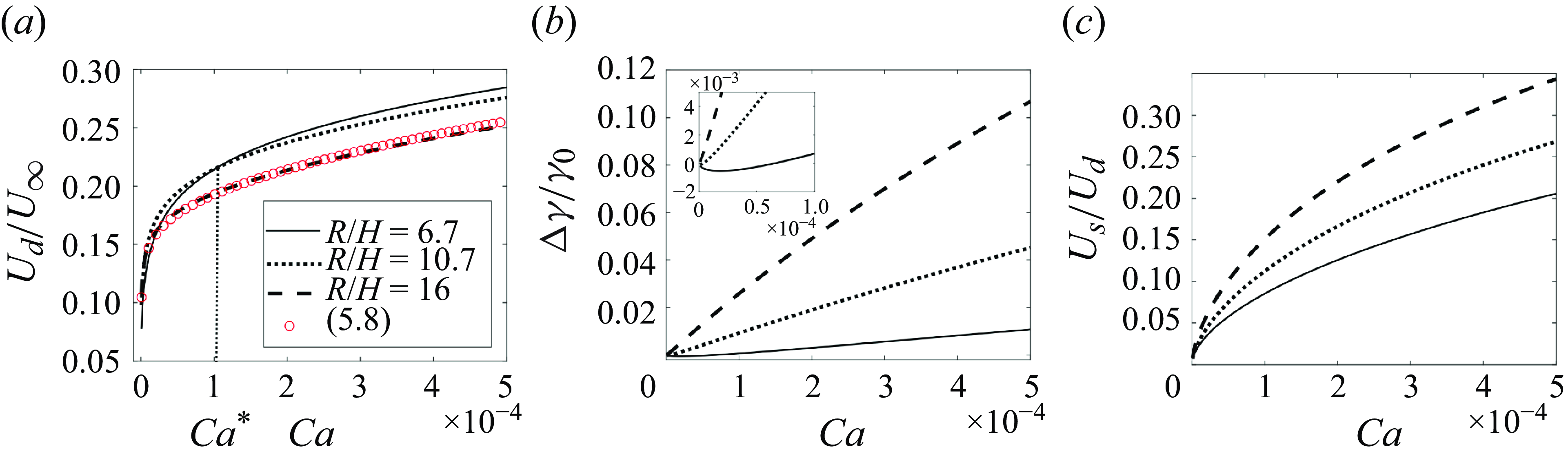
The drop mobility predicted by (C1) is shown in figure 9(a) as a function of
 $Ca$
for three values of
 $R/H$
. The simplified form (5.8) is plotted for
 $R/H=16$
and differs from the exact solution by a much smaller amount than our experimental error bars.
Theoretical value of the mobility
 $\beta$
(a), the surface tension variation
 $\Delta \gamma /\gamma _0$
(b) and the surface velocity
 $U_s/U_d$
(c), as a function of the capillary number
 $Ca$
for different aspect ratios
 $H/R$
. The black lines are the numerical results of (5.1)–(5.3) and the red circles are the simplified expression (5.8) for
 $R/H=16$
.

The first-order solution
 $U_d^0$
given by (5.7) is modified by corrections associated with (i) the classical Hele-Shaw flow, involving only the droplet aspect ratio and the viscosity ratio, (ii) the presence of the wetting film between the drop and the wall, identified by the prefactor
 $\zeta$
in (5.8) or equivalently by
 $U_s^0$
in (5.9), and (iii) the viscous force localised in the dynamical meniscus, identified by the prefactor
 $\xi$
.
The influence of the wetting film is firstly to increase the mobility through
 $U_s^0$
, which appears as a sliding velocity simply added to the first-order solution
 $U_d^0$
as is clear in the numerator of (5.9). However, this sliding velocity also modifies the spatial distribution of the surface tension around the drop and the relative velocity between the drop and the external fluid on the drop side. It thus modifies the surfactant transport in a complex way, thereby contributes to the denominator as well, which slows down the drop. The terms containing
 $U_s^0$
do not depend on the ratio
 $H/R$
but scale as
 $Ca^{2/3}$
, taking on more importance at large
 $Ca$
than the
 $H/R$
terms.
The meniscus contribution, proportional to
 $\xi$
, only appears in the denominator, and slows down the droplet. At small capillary number, it becomes dominant as it scales as
 $Ca^{-1/3}$
. In that limit, the droplet mobility scales as
 $\beta \sim Ca^{1/3} R/H$
and thus becomes an increasing function of the droplet radius. Equation (5.8) thus predicts a mobility decreasing with
 $R$
at large
 $Ca$
, dominated by the behaviour of
 $U_d^0$
(5.7) and increasing with
 $R$
at small
 $Ca$
, dominated by the meniscus friction.
We denote
 $Ca^*(R)$
the critical capillary number separating both regimes, as shown in figure 9(a). The curves associated with the values
 $R/H$
= 6.7 and 10.7 cross each other at
 $Ca^*\approx 10^{-4}$
and, as expected, the mobility is larger for the smaller radius at
 $Ca\gt Ca^*$
and the opposite is true for
 $Ca\lt Ca^*$
. The meniscus friction, which slows down the drop, dominates at small
 $Ca$
and is relatively more important for smaller droplets. At
 $Ca \gt Ca^*$
the surfactant transport from the rear to the front on the drop side is the limiting factor and the smaller droplets move faster.
The tension value is a key parameter in the problem and is shown in figure 9(b). Its value may increase by
 $10\%$
for the largest radius and capillary number investigated. Note that for a compressible interface having a Gibbs elasticity of the order of
 $\gamma _0$
, such tension increase would correspond to an interface extension of
 $10\%$
, which provides an indication of the accuracy of the incompressible interface assumption.
In the incompressible limit, this tension is a resistive force, adapting locally to maintain constant the local surfactant concentration (i.e. the local area). In order to provide an intuition of the tension sign, it is useful to determine how this concentration would vary without this constraint: if the concentration tends to decrease, the local tension is higher than at equilibrium, and the opposite if the concentration tends to increase. As for the droplet velocity, two different regimes can be identified:
(i) At large
 $Ca$
, the mobility is limited by the surfactant availability at the front: the drop motion tends to deplete the interface at the front, and the droplet must wait for the surfactant to arrive from the rear, on the drop side, to move. In that case the tension at the front is larger than at the rear and
 $\Delta \gamma \gt 0$
.
(ii) At small
 $Ca$
, however, the droplet mobility is limited by the friction in the meniscus. The surfactants on the drop side are pushed forward by the external flow, and they tend to accumulate at the front, waiting for the drop to move and to evacuate them at the interface of the wetting film: the surface tension is thus lower at the front than at the rear and
 $\Delta \gamma \lt 0$
. Note that, in this regime,
 $\Delta \gamma ^{film}$
remains positive, as well as the sliding velocity
 $U_s$
, shown in figure 9(c).
In our parameter range, the limiting factor is mainly the surfactant availability (case (i)), and the tension difference is positive for most values of
 $Ca$
. However, the friction regime (case (ii)) is observed at small
 $Ca$
, where the tension become slightly negative, as shown in the inset of figure 9(b).
5.3.
Alternative limit: solution for
 $\Delta \gamma =0$

The prediction (5.8) has been established for poorly soluble surfactants, for which the limit of an incompressible interface is expected to be reached. In the opposite limit, the surfactants adsorb or desorb fast enough to ensure a constant value of the surface tension. In that case, denoted as the stress-free case, another prediction for the droplet mobility can be obtained by adapting (5.1)–(5.3). The area conservation (5.3) is not satisfied any more and is replaced by the condition
 $\Delta \gamma = \Delta \gamma ^{film} =0$
. The parameter
 $\alpha$
becomes
 $\alpha =1$
in (5.1) and (5.2), and
 $\xi$
become zero in (5.1) and remains unchanged (
 $\xi$
= 1.19) in (5.2) (see Cantat Reference Cantat2013). Indeed,
 $\xi =0$
in the tension jump in the dynamical meniscus used in (4.17), whereas the viscous force exerted by the wall is still given by (4.19), with
 $\xi =1.19$
.
Thus, using
 $\Delta \gamma =0$
,
 $\xi = 0$
,
 $\alpha =1$
and
 $Ca \ll 1$
, (5.1) becomes
 \begin{equation} U_s= \frac {3 \eta _1}{\eta _2} \zeta (3 Ca)^{2/3} U_d \left (1 - \frac {3 \eta _1}{\eta _2} \zeta (3 Ca)^{2/3} \right ) \, . \end{equation}
Inserting
 $\Delta \gamma =0$
,
 $\alpha =1$
and
 $\xi =1.19$
, and the expression (5.10) of
 $U_s$
into (5.2) we get
 \begin{equation} \frac {U_d}{U_\infty } = \frac {2}{1+ \frac { \eta _1}{\eta _2} + \frac {8 \xi }{\pi } \frac {H}{R} (3 Ca)^{-1/3} - \left (\frac {\eta _1}{\eta _2}\right )^2 \zeta (3 Ca)^{2/3}} \approx \frac {2}{1+ \frac { \eta _1}{\eta _2} + K \frac {2 H}{R} Ca^{-1/3}} \; , \end{equation}
with
 $K= 4 \xi /(3^{1/3} \pi )=1.05$
. Therefore, we recover the expression established in Dangla (Reference Dangla2012) and for any
 $Ca$
, the mobility increases when the droplet radius increases. The parameter
 $K=1.05$
gives the theoretical value of the droplet mobility for a stress-free interface, thus providing an upper bound for the droplet mobility.
5.4. Comparison with the experiments

The experimental data of figure 4(h), obtained for
 $Ca= 5 \times 10^{-4}$
, are compared in figure 10 with model predictions for incompressible and stress-free interfaces, given respectively by (5.8) and (5.11). Note that these two predictions are built without any fitting parameter.
The mobilities of the less soluble surfactant are close to the prediction based on incompressible interfaces and decrease with the radius, as predicted by this model in the radius range of interest. The agreement is very good for droplets in the
 $C_{12}$
-sulphate and
 $C_{12}$
-bromide solutions. For some unexplained reason, the mobility in the
 $C_{14}$
-bromide solution, which has the lowest solubility, is further from the prediction, but the variation with
 $R$
is well reproduced.
For surfactants with shorter carbon chains, the mobility is significantly higher, the droplets being typically
 $50\, \%$
faster than with less soluble surfactants. When the carbon number decreases, the mobility curves get progressively closer to the other limiting model, based on stress-free interfaces. The mobility increases with the radius, as predicted by this second model, but the mobility value remains below the prediction, which appears as an upper limit for our data.
Finally, despite some experimental fluctuations, a robust trend can be identified from figure 10: the models of incompressible or stress-free interfaces provide a lower and an upper bound for the droplet mobility, the lower bound being reached for the carbon chains of 12 carbons or more. In the intermediate regime, the tension variations are non-negligible, but cannot be determined from the condition of incompressibility. The equations for the surfactant transport, coupled to the diffusion in the bulk, should thus in principle be solved.
The same conclusions can be drawn for figure 11, where the data from figure 4(a,e,f,g) are compared with the models.
The experimental mobility for the longest carbon chain are plotted in figures 11(a)–11(c) as a function of the capillary number for different radii. A quantitative agreement with the prediction of (5.8) is observed. This validates the key assumption of the model that the surfactant monolayer behaves as a 2-D incompressible fluid for low enough solubility. Importantly, in this regime, the drop mobility does not depend on any physico-chemical property of the interface. Indeed, this regime corresponds to the high Gibbs elasticity limit, and this key parameter, controlling the tension variation, thus scales out even if it dominates the dynamics.
The dependency with
 $R$
is small but significant at large
 $Ca$
, with a mobility decreasing with
 $R$
for a given
 $Ca$
, as more clearly shown in figure 10. By contrast, the model predicts that, for small
 $Ca$
, the mobility should increase with
 $R$
. The experimental noise is too large to verify this prediction, but the curves are closer to each other, especially in figure 11(a).
The mobility in the most soluble surfactant solution, the
 $C_8$
-sulphate, is also shown in figure 11(d) and compared with the prediction obtained using (5.11). As already visible in figure 10 the stress-free limit is not reached by this surfactant solution, but the dependency with
 $Ca$
and
 $R$
is very well captured.
Comparison between the experimental mobilities shown in figure 4(a,e,f,g) and prediction of the models. The symbols are experimental data obtained with (a) C
 $_{12}-$
sulphate, (b) C
 $_{12}-$
TAB and (c) C
 $_{14}-$
TAB, and the solid lines are the from (C1). The experimental data obtained with C
 $_8-$
sulphate are represented in (d) and the solid lines are obtained by solving (5.11) with
 $K=1.05$
.

6. Conclusion
In this paper, we performed several experiments to measure the mobility of confined droplets of fluorinatedoil pushed by an aqueous phase, as a function of the droplets size and of the surfactant solubility. Our experiments show an increase of mobility with the capillary number
 $Ca$
and with the radii of the droplets for C
 $_8-$
sulphate, C
 $_{10}-$
sulphate, C
 $_{10}-$
TAB and C
 $_{11}-$
sulphate. However, for C
 $_{12}-$
sulphate, C
 $_{12}-$
TAB and C
 $_{14}-$
TAB, the mobility observed decreases when the radius of the droplet increases. We propose an original model that distinguishes between two limiting situations: a stress-free interface and an incompressible interface. These two limiting cases make it possible to bound the mobility of a droplet as a function of the solubility of the surfactant used. Importantly, the limit based on the assumption of interface incompressibility leads to an analytical prediction of the droplet velocity as a function of the droplet radius and as a function of the capillary number. The excellent agreement between the experimental data and the theory validates the key assumption of interface incompressibility we made: in the investigated regime, and for low enough solubility, the interface Gibbs elasticity is large enough to preclude any area variation at the interface. As such, this work identifies a new regime of droplet transport in a Hele-Shaw cell, in which the motion is limited by the surfactant flux on the lateral sides of the droplet, and by the surface tension difference between the front and the rear. Interestingly, the model should be valid for any surfactant less soluble than the one we used, and give quantitative predictions for the droplet velocity. Conversely, although a maximum velocity is obtained for a stress-free interface, prediction for surfactants of intermediate solubility requires taking into account the full transport of surfactants.
Acknowledgements.
The authors are grateful to A. Saint-Jalmes for fruitful discussions and surface tension and rheological measurements, E. Schaub for fruitful discussions and P. Chasle for technical support. The theoretical part of this project was partly carried out at the DAMTP, thanks to the hospitality of R. Goldstein and of Churchill college, Cambridge, UK.
Funding.
This work was supported by CNRS, Université de Rennes, Région Bretagne, Rennes Métropole and Agence Nationale de la Recherche (ANR) under the grant ANR-18-CE09-0029.
Declaration of interests.
The authors report no conflict of interest.
Appendix A
The general expression of the velocity field in the external and internal phases is given by (4.8). The parameters
 $a$
,
 $b$
,
 $c$
,
 $d$
and
 $e$
are computed in Gallaire et al. (Reference Gallaire, Meliga, Laure and Baroud2014) for three cases: (i) a Marangoni stress on the lateral side of a static drop, without far field velocity, (ii) a static drop having a uniform surface tension, with far field velocity, and finally (iii) a translating drop, with a uniform tension and without far field velocity. Our case is recovered from a linear superposition of these 3 cases. In the following, each equation X or parameter
 $a$
of Gallaire et al. (Reference Gallaire, Meliga, Laure and Baroud2014) will be denoted (XG) or
 $a^G$
in the following (especially the parameters
 $a^G$
,
 $b^G$
,
 $c^G$
,
 $d^G$
and
 $e^G$
which differ from our notation).
For the Marangoni forcing (i), the parameters are defined in (27G) and (28G) and their values are given by the dimensionless equations (29G), (30G) and (31G). The associated dimensions are
 $R$
,
 $(\eta _1+\eta _2) R/\Delta \gamma$
and
 $\Delta \gamma R$
for the length, time and force. In the limit of large drop radius that we consider,
 $K_n(k) \sim \sqrt {\pi /(2k)} e^{-k}$
and
 $I_n(k) \sim \sqrt {1/(2\unicode{x03C0} k)} e^{k}$
for any order
 $n$
, and for our sinusoidal forcing, only the
 $\sin \theta$
component is non-zero. Equation (31G) becomes
 \begin{equation} d_1^G = - \frac {\sqrt {3} R}{2H} \; . \end{equation}
The forcing
 $a_1^G$
in (29G) is defined from
 $\gamma = - a_1^G (\Delta \gamma ) \cos \theta + \gamma _0$
(7G) and is thus
 $a_1^G= -1$
in our case. Hence, the parameters
 $a^M$
,
 $b^M$
,
 $c^M$
,
 $d^M$
and
 $e^M$
associated with the velocity field induced by the surface tension gradient are obtained from (29G), (30G)
 \begin{equation} a^M = \frac {R \Delta \gamma }{\eta _1 + \eta _2} \frac {H^2}{3 R^2} \quad , \quad b^M = c^M = -d^M = -a^M \quad , \quad e^M =0 \; . \end{equation}
For a far field velocity
 $U_\infty$
, case (ii), the units chosen in Gallaire et al. (Reference Gallaire, Meliga, Laure and Baroud2014) are
 $R$
,
 $R/U_\infty$
and
 $R (\eta _1+ \eta _2) U_\infty$
for the length, time and force. The parameters of the velocity field are deduced from (49G)–(53G)
 \begin{align} a^\infty &= \frac {\eta _2}{\eta _1+\eta _2} \frac {2 H U_\infty }{\sqrt {3}} \quad , \quad b^\infty = -a^\infty \, , \nonumber \\ c^\infty &= \frac {\eta _1}{\eta _1+\eta _2} \frac {2 H U_\infty }{\sqrt {3}} \quad , \quad d^\infty = -c^\infty - R U_\infty \quad , \quad e^\infty = R U_\infty \; . \end{align}
Finally the case (iii) of a drop moving at the velocity
 $U_d$
(chosen to be negative in Gallaire et al. (Reference Gallaire, Meliga, Laure and Baroud2014)) is solved with the dimension set
 $R$
,
 $- R/U_d$
and
 $- R (\eta _1+ \eta _2) U_d$
for the length, time and force.
The parameters are deduced from (59G)–(62G)
 \begin{align} a^D &=-\frac {\eta _2}{\eta _1+\eta _2} \frac {2 H U_d}{\sqrt {3}} , \quad b^D = -a^D + U_d R, \nonumber \\ c^D & = - \frac {\eta _1}{\eta _1+\eta _2} \frac {2 H U_d}{\sqrt {3}}, \quad d^D = -c^D + R U_d, \quad e^D=0 \, . \end{align}
The parameters of our streamfunctions are finally obtained by summing the three contributions
 \begin{align} &a= \frac {R \Delta \gamma }{\eta _1 + \eta _2} \frac {H^2}{3 R^2} + \frac {\eta _2}{\eta _1+\eta _2} \frac {2 H }{\sqrt {3}}(U_\infty -U_d ), \nonumber \\ &b= - \frac {R \Delta \gamma }{\eta _1 + \eta _2} \frac {H^2}{3 R^2} -\frac {\eta _2}{\eta _1+\eta _2} \frac {2 H}{\sqrt {3}}( U_\infty -U_d) + U_d R,\nonumber \\ &c= -\frac {R \Delta \gamma }{\eta _1 + \eta _2} \frac {H^2}{3 R^2} + \frac {\eta _1}{\eta _1+\eta _2} \frac {2 H }{\sqrt {3}}(U_\infty -U_d ), \nonumber \\ &d= \frac {R \Delta \gamma }{\eta _1 + \eta _2} \frac {H^2}{3 R^2} -\frac {\eta _1}{\eta _1+\eta _2} \frac {2 H}{\sqrt {3}}( U_\infty -U_d) - R (U_\infty -U_d), \nonumber \\ & e= R U_\infty. \end{align}
Appendix B
The tangential velocity is
 $u_\theta = - \partial _r \psi$
, so the velocity at the point
 $(R, \pi /2)$
, projected in the
 $x$
direction, is
 $u^{lat} = \partial _r \psi (R,\pi /2)$
. Using the relation
 \begin{equation} \frac {{\rm d}I_1(x)}{{\rm d}dx} = I_2(x)+ \frac {1}{x} I_1(x) \quad \mbox {and} \quad \frac {{\rm d}K_1(x)}{{\rm d}x} = - K_0(x) - \frac {1}{x} K_1(x) \, , \end{equation}
we get
 \begin{align} \partial _r \Psi _1 & = \left ( \frac {a}{I_1(k)}\left ( k I_2(kr/R)+ \frac {R}{r} I_1(kr/R) \right ) + b \right ) \frac {\sin \theta }{R} \, ,\end{align}
 \begin{align} \partial _r \Psi _2 & = \left (\frac {c}{K_1(k)} \left ( - k K_0(kr/R) - \frac {R}{r} K_1(kr/R)\right ) - d \frac {R^2}{r^2} + e \right ) \frac {\sin \theta }{R} \, .\end{align}
In the limit of large
 $k$
, we get
 \begin{equation} u^{lat} = (ak+b) \frac {1}{R} = (-ck-d+e) \frac {1}{R} \, , \end{equation}
leading to (4.21).
Appendix C
The inversion of the system of (5.1)–(5.3) leads to the solution
 \begin{equation} \beta = \frac {U_d}{U_\infty } = \frac {num}{denom} \, , \end{equation}
with
 \begin{align} num & = \frac {H}{R} \frac {2 \eta _2}{\eta _1 + \eta _2} \left (1 +\sqrt {3} \right ) + \frac {H^2}{R^2} \frac {4 \eta _2^2}{(\eta _1 + \eta _2)^2}\nonumber\\& \quad + 6 \zeta (12 Ca)^{2/3} \left ( 1 + \frac {\sqrt {3} \eta _1}{\eta _1+ \eta _2} \frac {H}{R}+ \frac {2 \eta _1 \eta _2}{(\eta _1+\eta _2)^2} \frac {H^2}{R^2} \right ) \nonumber \\ &= \frac {U_d^0}{U_\infty } + \frac {U_s^0}{U_\infty } \left ( 1 + \frac {\sqrt {3} \eta _1}{\eta _1+ \eta _2} \frac {H}{R}+ \frac {2 \eta _1 \eta _2}{(\eta _1+\eta _2)^2} \frac {H^2}{R^2} \right ) + \frac {H^2}{R^2} \frac {4 \eta _2^2}{(\eta _1 + \eta _2)^2} ,\end{align}
and
 \begin{align} denom & = 1 + \frac {H}{R} \frac { \eta _2}{\eta _1+ \eta _2} \left ( \sqrt {3}+ 4 + \frac {\sqrt {3} \eta _1}{\eta _2} \right ) + \frac {H^2}{R^2} \frac {\eta _2}{\eta _1+ \eta _2} \frac {2 \sqrt {3} \xi }{ (12 Ca)^{1/3}} \left ( \frac {4}{\pi } + 1 \right ) \nonumber \\ & \quad + 3 \zeta (12 Ca)^{2/3} + \frac {H}{R} \frac {24 \xi \zeta }{\pi } (12 Ca)^{1/3} +\frac {4 \eta _2^2}{(\eta _1+ \eta _2)^2} \frac {H^2}{R^2} \nonumber \\ & \quad + \frac {3 \sqrt {3} \eta _1}{\eta _1+\eta _2} \frac {H}{R} \zeta (12 Ca)^{2/3} + 12 \xi \zeta (12 Ca)^{1/3} \frac {H^2}{R^2} \frac { \sqrt {3} \eta _1}{\eta _1+ \eta _2} \left ( \frac {2\sqrt {3}}{\pi } - \frac {\eta _2}{\eta _1} \right ) \nonumber \\ & \quad +\frac {12 \eta _1 \eta _2}{(\eta _1 + \eta _2)^2} \frac {H^2}{R^2} \zeta (12 Ca)^{2/3} \, . \end{align}