






1. Introduction
Turbulent boundary layer (TBL) flows exhibit significant complexity, which is reflected in the wide range of energetic scales that contribute to the spectrum of the streamwise velocity (Saddoughi & Veeravalli Reference Saddoughi and Veeravalli1994; Jiménez Reference Jiménez2012; Cardesa, Vela-Martín & Jiménez Reference Cardesa, Vela-Martín and Jiménez2017). Statistical analysis reveals that amid this complexity and chaotic behaviour, certain consistent and widespread structural features, such as vortices, ramp-like shear layers, outer layer streaks, weakly rotating rolls and large sweep/ejection events, emerge (Cantwell Reference Cantwell1981; Robinson Reference Robinson1991; Adrian Reference Adrian2007; Dennis & Nickels Reference Dennis and Nickels2011; Jiménez Reference Jiménez2018; Heisel et al. Reference Heisel, de Silva, Hutchins, Marusic and Guala2021). One of the manifestations of these structural features on the instantaneous flow fields is the occurrence of regions of nearly uniform streamwise velocity, defined as uniform momentum zones (UMZs), separated by internal shear layers (ISL), also referred to as vortical fissures (VFs) (Priyadarshana et al. Reference Priyadarshana, Klewicki, Treat and Foss2007; Eisma et al. Reference Eisma, Westerweel, Ooms and Elsinga2015; de Silva, Hutchins & Marusic Reference de Silva, Hutchins and Marusic2016; de Silva et al. Reference de Silva, Philip, Hutchins and Marusic2017; Heisel et al. Reference Heisel, de Silva, Hutchins, Marusic and Guala2020; Iungo et al. Reference Iungo, Guala, Hong, Bristow, Puccioni, Hartford, Ehsani, Letizia, Li and Moss2024).
Adopting these flow features and leveraging on their governing scaling laws has led to the formulation of simplified models aimed at reducing the computational costs of wall-turbulence flow simulations (Perry & Chong Reference Perry and Chong1982; Klewicki & Oberlack Reference Klewicki and Oberlack2015; Bautista et al. Reference Bautista, Ebadi, White, Chini and Klewicki2019; Marusic & Monty Reference Marusic and Monty2019; Ehsani et al. Reference Ehsani, Heisel, Li, Voller, Hong and Guala2024).
Uniform momentum zones, in particular, have been detected in spatial measurements of turbulent boundary layer flows, conducted in both laboratory and field settings, and linked to the evolution of wall-attached, large-scale structures in the outer layer (Meinhart & Adrian Reference Meinhart and Adrian1995; Adrian, Meinhart & Tomkins Reference Adrian, Meinhart and Tomkins2000; Heisel et al. Reference Heisel, Dasari, Liu, Hong, Coletti and Guala2018).
The vertical distribution of UMZs and shear layers results in the step-like shape of the instantaneous velocity profile, up to the turbulent–non-turbulent interface (de Silva et al. Reference de Silva, Hutchins and Marusic2016; Heisel et al. Reference Heisel, de Silva, Hutchins, Marusic and Guala2020). In the logarithmic region, the thickness of the internal shear layers was observed to scale with the Taylor microscale  $\delta _{\omega } \approx 0.4\lambda _{T}$ (Eisma et al. Reference Eisma, Westerweel, Ooms and Elsinga2015; de Silva et al. Reference de Silva, Philip, Hutchins and Marusic2017; Heisel et al. Reference Heisel, de Silva, Hutchins, Marusic and Guala2021), while the local velocity difference, or jump, was found to scale with the friction velocity
 $(\Delta U_{m} \approx 2u_{\tau })$ (de Silva et al. Reference de Silva, Philip, Hutchins and Marusic2017; Heisel et al. Reference Heisel, Dasari, Liu, Hong, Coletti and Guala2018). It was also shown that, within the logarithmic region, the thickness of UMZs scales with the wall-normal distance
 $(H_{m} \approx z)$ (Heisel et al. Reference Heisel, de Silva, Hutchins, Marusic and Guala2020; Ehsani et al. Reference Ehsani, Heisel, Li, Voller, Hong and Guala2024). This scaling behaviour is consistent with the hairpin paradigm phenomenological model (Adrian Reference Adrian2007) and with the attached eddy hypothesis (AEH), which assumes the size of self-similar turbulent motions to scale with the distance from the wall (Townsend Reference Townsend1976; de Silva et al. Reference de Silva, Hutchins and Marusic2016; Marusic & Monty Reference Marusic and Monty2019; Deshpande, de Silva & Marusic Reference Deshpande, de Silva and Marusic2023).
The analysis of the statistical moments computed on a large ensemble of UMZ profiles, extracted from canonical turbulent boundary layer flows, demonstrated the preservation of the mean and root-mean-square (r.m.s.) streamwise velocity in the logarithmic region (Heisel et al. Reference Heisel, Dasari, Liu, Hong, Coletti and Guala2018; Ehsani et al. Reference Ehsani, Heisel, Li, Voller, Hong and Guala2024). Hence, the UMZs, along with their accompanying shear layers, can be interpreted as a ubiquitous, fundamental signature of the attached-eddy coherent structures, which are linked to the momentum transfer and other surface processes in turbulent boundary layers across various surface roughness conditions and Reynolds numbers (Prandtl Reference Prandtl1925; Heisel et al. Reference Heisel, Dasari, Liu, Hong, Coletti and Guala2018, Reference Heisel, de Silva, Hutchins, Marusic and Guala2020; Bautista et al. Reference Bautista, Ebadi, White, Chini and Klewicki2019; Bross, Fuchs & Kähler Reference Bross, Fuchs and Kähler2019; Xu, Zhong & Zhang Reference Xu, Zhong and Zhang2019; Cogo et al. Reference Cogo, Salvadore, Picano and Bernardini2022; Puccioni et al. Reference Puccioni, Calaf, Pardyjak, Hoch, Morrison, Perelet and Iungo2023; Salesky Reference Salesky2023; Zhang et al. Reference Zhang, Li, Su and Jiang2023).
The vertical variability of UMZs and shear layers, manifested in the observed different step-like instantaneous profiles extracted from experimental data, can be thus used to reproduce the streamwise and vertical velocity variability in wall turbulent flows. Leveraging on this observation, various approaches, often encompassing theoretical assumptions and experimental data assimilation techniques, have been proposed to generate synthetic instantaneous velocity profiles, with a more or less complex spatio-temporal distribution, as computationally inexpensive, low-dimensional models of wall turbulence (Perry & Chong Reference Perry and Chong1982; McKeon & Sharma Reference McKeon and Sharma2010; Saxton-Fox & McKeon Reference Saxton-Fox and McKeon2017; Bautista et al. Reference Bautista, Ebadi, White, Chini and Klewicki2019; Ehsani et al. Reference Ehsani, Heisel, Li, Voller, Hong and Guala2024).
Ehsani et al. (Reference Ehsani, Heisel, Li, Voller, Hong and Guala2024) used laboratory (wind tunnel) and field scale atmospheric surface layer (ASL) measurements in rough-wall turbulent boundary layers to extract the wall-normal location, kinematic and geometrical properties of UMZs. These include the thickness  $h_m$, the modal velocity
 $u_m$, the vertically averaged velocity
 $w_m$ and the mid-height elevation
 $z_m$. All these attributes have been re-organized and statistically characterized as a function of
 $z$. Leveraging on the resulting first and second statistical moments of UMZ attributes, a set of models has been proposed to stochastically generate one-dimensional (1-D) step-like instantaneous modal (streamwise) and vertical velocity profiles. These are based on the inverse transform sampling technique, inverting the cumulative density functions to sample each corresponding attribute, and on a prescribed correlation coefficient to capture the correct Reynolds shear stress
 $\langle u'_m w'_m\rangle$. Results show that the ensemble of stochastically generated profiles reproduces the mean velocity and variances of canonical rough-wall turbulent boundary layers, including some key structural features as the attached-eddy scaling of UMZ thickness (Heisel et al. Reference Heisel, de Silva, Hutchins, Marusic and Guala2020) and the shear velocity scaling of the velocity jump across UMZ interfaces (Heisel et al. Reference Heisel, de Silva, Hutchins, Marusic and Guala2021). The primary reason for selecting the log region as the focus of our work is to ensure the scalability of our modelling approach, especially towards high-Reynolds-number flows. The log region is ubiquitous, and its thickness increases in the ASL creating the space and opportunity for bottom-up wall modelling. By recalling the mixing length assumption in the derivation of the logarithmic law of the wall, and its relation to UMZ thickness (as discussed by Heisel et al. Reference Heisel, de Silva, Hutchins, Marusic and Guala2020), we hope that the predictive capabilities of this model can extend as high as the log layer can reach.
In the present work, we first re-order the generated 1-D rough-wall turbulent profiles into a two-dimensional (2-D) modal velocity field, and then we extend the comparison with measured wall turbulent flows to account for turbulent kinetic energy (TKE) production, dissipation and scale-dependent streamwise velocity variance, i.e. the power spectrum.
To introduce some small-scale turbulence, and allow for the continuity of the modal velocity vertical gradients, shear layers with prescribed thickness were introduced in the stochastically generated profiles, replacing the abrupt velocity jump of each step. To opportunely order and set the spatial (or temporal) resolution of the generated profiles, hot-wire datasets from the wind tunnel measurements (Heisel et al. Reference Heisel, de Silva, Hutchins, Marusic and Guala2020) and sonic datasets from ASL measurements (Iungo et al. Reference Iungo, Guala, Hong, Bristow, Puccioni, Hartford, Ehsani, Letizia, Li and Moss2024) were used (§ 2). The consistency of the generated and rearranged spatial velocity field with the measured turbulent boundary layer flows is assessed across a wide range of Reynolds numbers in § 3, and conclusions follow in § 4.
In this study, the symbol  $z$ denotes the wall-normal distance and the subscript ‘
 $i$’ denotes an arbitrary elevation
 $z_{i}$ or a UMZ attribute at any given location, e.g. the modal velocity
 $u_{m_{i}}$. The subscript ‘
 $m$’ is used to distinguish attributes of UMZs, such as
 $u_m$ or
 $h_m$. The superscript ‘
 $+$’ marks inner unit normalization,
 $u^+=u/u_{\tau }$. For variables, lowercase lettering indicates instantaneous value, while uppercase lettering defines the temporal, spatial or ensemble averages. For velocity, superscript
 $'$ denotes fluctuations from the mean value according to the Reynolds decomposition
 $u=U+u^{'}$.
2. Methodology
2.1. UMZ detection and profile generation
The UMZ detection and extraction procedure, required to guide the modal velocity profile generation, was implemented on three experimental datasets and described in detail by Heisel et al. (Reference Heisel, de Silva, Hutchins, Marusic and Guala2020). Instantaneous spatial and temporal velocity fields were obtained from particle image velocimetry (PIV) and hot-wire measurements, respectively, obtained in the St. Anthony Fall Laboratory atmospheric boundary layer wind tunnel, under approximately zero pressure gradient conditions (Heisel et al. Reference Heisel, de Silva, Hutchins, Marusic and Guala2020). In addition, we used field measurements in the ASL performed at the Eolos Wind Research Field Station in Rosemount, Minnesota (Iungo et al. Reference Iungo, Guala, Hong, Bristow, Puccioni, Hartford, Ehsani, Letizia, Li and Moss2024), employing super-large-scale particle image velocimetry (SLPIV, Toloui et al. Reference Toloui, Riley, Hong, Howard, Chamorro, Guala and Tucker2014) and sonic anemometer measurements. The two wind tunnel datasets, labelled as m1 and m2, are characterized by fully rough conditions induced by a horizontal steel wire mesh. The experimental measurements collected by hot-wire are denoted by H-W(m1) and H-W(m2) throughout the paper. The details about the turbulent flow characteristics and the experiment's parameters are presented in table 1. In the following, we provide a brief summary of how instantaneous velocity profiles have been generated using UMZ distribution obtained from experimental data. The details are presented by Ehsani et al. (Reference Ehsani, Heisel, Li, Voller, Hong and Guala2024). Uniform momentum zones were identified using the histogram-based approach, which was first introduced by Adrian et al. (Reference Adrian, Meinhart and Tomkins2000), and recently implemented by de Silva et al. (Reference de Silva, Hutchins and Marusic2016), Heisel et al. (Reference Heisel, de Silva, Hutchins, Marusic and Guala2020) and Ehsani et al. (Reference Ehsani, Heisel, Li, Voller, Hong and Guala2024). Figure 1(a) illustrates the results of the UMZ detection algorithm, with each distinct UMZ depicted in a unique colour. The black solid curve represents the shear interface between neighbouring UMZs. For the stochastic generation of modal velocity profiles, a comprehensive statistical analysis of UMZ characteristics (i.e. thickness  $h_{m_{i}}$, modal velocity
 $u_{m_{i}}$ and vertical velocity
 $w_{m_{i}}$) at each generic wall-normal location is required. At each given
 $z_{i}$, cyan dashed line in figure 1(a), we group all UMZs that intersect
 $z_{i}$; four samples of them shown by the double circle head vertical yellow lines. This way, we obtain a distribution of UMZ characteristics even near the wall, whose mid-height elevation is larger than the elevation reference location (
 $z_{m_{i}}>z_{i}$). The distribution of
 $h_{m}$ and
 $u_{m}$ for the specified wall-normal location
 $z_{i}$ is depicted in figure 1(b,c). The distribution of the UMZs thickness is classified as log-normal, while the distribution of the modal velocity and vertical velocity is approximated as Gaussian (Ehsani et al. Reference Ehsani, Heisel, Li, Voller, Hong and Guala2024).
Experimental dataset used in calculating autocorrelation, shear layer thickness and making a comparison with the generated velocity field.

Illustrated procedure for the stochastic generation of modal velocity profiles. (a) Mapped UMZ from instantaneous experimentally obtained velocity field using histogram-based approach. Thickness  $h_{m_{i}}$, mid-height elevation
 $z_{m_{i}}$ and modal velocities
 $u_{m_{i}}$ for the detected UMZs. Double circle head yellow vertical lines indicate sampled thicknesses
 $h_{m_{i}}$ of the UMZs intersecting the generic height
 $z_{i}$ (dashed cyan horizontal line) for which the statistics of UMZ characteristics are collected. (b) Probability density function (p.d.f.) of the UMZ thickness
 $h_m$. (c) P.d.f. of UMZ modal velocity
 $u_m$. (d) Reproduced cumulative distribution function (c.d.f.) of
 $h_m$. (e) Reproduced c.d.f. of
 $u_m$. (f) A sample step of the stochastically generated velocity profile.

Leveraging on the statistics of the UMZ attributes, we can reconstruct their height-dependent cumulative distribution functions (c.d.f.s), which are critical for the stochastic generation procedure of instantaneous step-like velocity profiles. Let us suppose we are located at the specific wall-normal location at  $z_{i}$, as shown in figure 1(f). Using the extracted statistics of the
 $h_m$ thickness at
 $z_{i}$, we are able to reproduce the c.d.f. of
 $h_m$ at this location, as plotted in figure 1(d). A random number between 0 and 1 is then sampled out of a uniform distribution
 $r_{h_{m_{i}}} \in (0\ 1)$. The thickness
 $h_{m_{i}}$ of the generated UMZ is determined by inverting the cumulative distribution function of the log-normal distribution. This approach is known as inverse transform sampling and has been used in different research areas (Foufoula-Georgiou & Stark Reference Foufoula-Georgiou and Stark2010; Fan et al. Reference Fan, Singh, Guala, Foufoula-Georgiou and Wu2016; Heisel Reference Heisel2022). The technique for determining the modal and vertical velocities of the generated UMZ is similar, except that it uses statistics from the mid-height elevation
 $z_{m_{i}} = z_{i}+h_{m_{i}}/2$ of the generated UMZ to reconstruct the cumulative distribution function of
 $u_m$ and
 $w_m$ to invert. For the purpose of reproducing the Reynolds shear stress
 $-\overline {u^{\prime }w^{\prime }}$, the random numbers used for
 $r_{u_{m_{i}}}$ and
 $r_{w_{m_{i}}}$ are from a Gaussian copula with an imposed linear correlation parameter. This approach guarantees a specified Pearson correlation coefficient and ensures that both variables are uniformly distributed within the range
 $\in (0\ 1)$ (Joe Reference Joe1997; Nelsen Reference Nelsen2007). The stochastically generated modal velocity profile shown in figure 1(f) is just one of the many step-like profiles generated by the model. One of the technical reasons we focused on the log region is the invariance of the Reynolds shear stress
 $({\partial u^{\prime }w^{\prime }}/{\partial z} \approx 0)$, and the balance of TKE production and dissipation in this region, which facilitate the development and validation of our model. The linear variation in UMZs thickness with elevation and the known parametrization of the mean velocity profile allow us to normalize UMZ statistics across a wide range of Reynolds numbers and assess the representativeness of our model (Heisel et al. Reference Heisel, de Silva, Hutchins, Marusic and Guala2020; Ehsani et al. Reference Ehsani, Heisel, Li, Voller, Hong and Guala2024). Ehsani et al. (Reference Ehsani, Heisel, Li, Voller, Hong and Guala2024) demonstrated that a large enough ensemble of generated modal velocity profiles effectively reproduce the statistical moments of canonical rough-wall turbulent boundary layer flows and exhibit statistical characteristics of wall-attached behaviour within the logarithmic region.
2.2. Introducing a finite size shear layer
Modal velocity profiles are generated stochastically, by inverse transform sampling of the UMZ thickness  $h_m$ and modal velocity
 $u_m$ distributions, as described by Ehsani et al. (Reference Ehsani, Heisel, Li, Voller, Hong and Guala2024) and sketched in figure 1(f). These profiles necessarily exhibit a step-like shape: the resulting internal shear layers (ISLs) had zero thickness (figure 2a) and locally infinite velocity gradients.
Modal velocity profile. (a) Shear layers with zero thickness. (b) Modified shear layers with thickness  $\delta _{\omega }$. The sampled internal shear layer coloured in purple is described by (2.1).

Our first objective is to identify an appropriate length scale, introduce a smooth transitional region between adjacent UMZs, and reproduce the correct streamwise velocity profile in the ISLs. Using PIV measurements (Heisel et al. Reference Heisel, de Silva, Hutchins, Marusic and Guala2021) was able to estimate statistically the ISL thickness,  $\delta _{\omega }$, at different elevations
 $z/\delta$ in rough-wall turbulent boundary layers. From those results, the ratio between
 $\delta _{\omega }$ and the Taylor microscale,
 $\delta _{\omega }/\lambda _{T}\simeq 0.4$, was observed to be fairly invariant throughout the outer layer, as previously observed by Eisma et al. (Reference Eisma, Westerweel, Ooms and Elsinga2015) and de Silva et al. (Reference de Silva, Philip, Hutchins and Marusic2017) over smooth surfaces. Based on the above results, we used the high-frequency hot-wire dataset from the wind tunnel experiments by Heisel et al. (Reference Heisel, de Silva, Hutchins, Marusic and Guala2020) and the sonic and SLPIV measurements from a recent ASL dataset (Iungo et al. Reference Iungo, Guala, Hong, Bristow, Puccioni, Hartford, Ehsani, Letizia, Li and Moss2024) to determine the Taylor micro-scale, and imposed the thickness of the ISL as
 $\delta \omega =0.4\lambda _T$ (Heisel et al. Reference Heisel, de Silva, Hutchins, Marusic and Guala2021). The shape of the velocity profile in the finite shear layers can now be defined by a modified ellipsoid equation, as a function of the length scale
 $\lambda _{T}$ and the velocity jump
 $\Delta u$ as described in figure 2(b). This formulation is inspired by the Oseen vortex equation describing advecting and rotating 2-D vortex cores (Oseen Reference Oseen1912). Heisel et al. (Reference Heisel, de Silva, Hutchins, Marusic and Guala2021) inferred that both the ISL and the energetic prograde vortex cores can be statistically described by the same scaling quantities: the largest vortex core diameter varying with
 $\lambda _{T}$ and the azimuthal velocity scaling with
 $u_{\tau }$, which can be easily implemented as semi-axes in the elliptic shear layer equation. In addition, Heisel et al. (Reference Heisel, Dasari, Liu, Hong, Coletti and Guala2018) demonstrated that vortex cores in the logarithmic region are preferentially located within the ISL, thus supporting a consistent mathematical formulation. Equation (2.1) is then implemented to introduce finite internal shear layers into the modal velocity step-like profiles.
 \begin{equation} \left.\begin{array}{ll@{}}
u^+_{{ISL_{i}}} = u^+_{m_{i}}+\dfrac{\Delta u^+_{m_{i}}}{2} [(1-\cos{\theta}), (\sin{\theta}+1)]\\
\dfrac{z_{{ISL_{i}}}}{\delta} = \dfrac{z_{{ISL_{c_{i}}}}}{\delta}+\dfrac{\delta_{\omega}}{2\delta} [(\sin{\theta}-1), (1-\cos{\theta})] \!\!\end{array}\right\} \quad 0 \le \theta \le \frac{\rm \pi}{2} \end{equation}
Here,  $u^+_{m_{i}}$ denotes the modal velocity of the
 $i$th UMZ, as shown in figure 2(a);
 $u^+_{{ISL_{i}}}$ represents the flow velocity at the midpoints of the internal shear layer, in between two UMZs, as depicted in figure 2(b);
 $\Delta u_{m_{i}}$ is the velocity jump (i.e. the difference in modal velocity between two neighbouring UMZs), resulting from the stochastic generation process. The corresponding wall-normal location
 ${z_{{ISL_{i}}}}/{\delta }$ depends on the mid-elevation of the ISL,
 ${z_{{ISL_{c_{i}}}}}/{\delta }$, and thickness of the shear layer,
 $\delta _{\omega }$. The shear layer thickness is imposed using the local,
 $z$-dependent, Taylor micro-scale, using the scaling relationship
 $\delta _{\omega }=0.4\lambda _T$ suggested by Heisel et al. (Reference Heisel, de Silva, Hutchins, Marusic and Guala2021). Two harmonic functions are employed to describe both the lower and upper portion of the velocity profile, within the ISL, relative to its mid-elevation
 ${z_{{ISL_{c_{i}}}}}/{\delta }$ (see figure 2).
2.3. Combining velocity profiles into a modal velocity spatial field
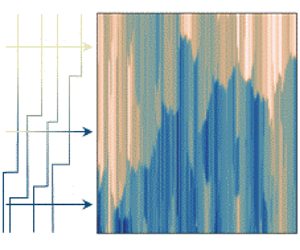
Our next objective is to arrange the independent, stochastically generated, modal velocity profiles into a spatially (or temporally) coherent, realistic, velocity field. We follow a procedure inspired by the approach introduced by Cazanacli (Reference Cazanacli2021) to reconstruct channelization and avulsions in fluvial dispositional systems (Bryant, Falk & Paola Reference Bryant, Falk and Paola1995). Initially, we select a single starting modal velocity profile, randomly, from a set of  $N$ generated modal velocity profiles (figure 3 first step). The collection of profiles is referred to as Repository (figure 3), and
 $N$ can potentially be unrestricted. To determine the second modal velocity profile of the generated velocity field, an additional set of independent modal velocity profiles, of finite size
 $M< N$, is required. This set of profiles is referred to as Storage, and its size is assumed, for now, to be contingent upon the Reynolds number
 $Re_\tau$ of the synthetic velocity field we are constructing. The
 $Re_\tau$ dependency of Storage size will be discussed in § 3.9. To introduce spatial coherence in the velocity field, we compute the cross-correlation coefficient between the first profile
 $u_{m1}(z)$ of the modal velocity field and all the profiles in the Storage
 $u_{mi}(z)$ (figure 3 second step). This enables us to identify the profile with the highest correlation (among the
 $M$ samples), which is then designated as the second profile in the modal velocity field, and so on (figure 3 third step). Due to the finite size of the Storage and the limited vertical extent of the shear layers in the generated velocity profiles, the choice of modelling the finite shear layer, as opposed to the sharp interface implemented by Ehsani et al. (Reference Ehsani, Heisel, Li, Voller, Hong and Guala2024), was observed to have a negligible effect on the process of selecting the most correlated velocity profile. The second profile is then removed from Storage and replaced with a randomly selected velocity profile from the Repository (figure 3 fourth step). This process ensures a consistent number of profiles within the Storage. Our methodology entails continuous sampling from the Storage, selecting the most correlated velocity profile with respect to the latest addition to the velocity field (steps 2 and 3), and replacing the chosen profile with a randomly selected one from the Repository (step 4). The process of replenishing the Storage with a random profile from the Repository yields the following outcomes.
Model procedure for making the velocity field. The size of the Repository and the velocity field are undefined. The size of Storage is limited and the Reynolds number dependent.

(i) It ensures a consistent number of profiles  $M$, so that the selection and the reordering process are not compromised by a progressively reduced number of available samples. This ensures the statistical homogeneity (steadiness) in the reordered spatial (temporal) velocity field.
(ii) During the iteration, the random replacement of profiles keeps introducing variability in the Storage, which periodically triggers more abrupt changes in the vertical structure of the profiles, and in fact creates some very-large-scale excursions in the velocity field. Because of the continuous search for nearly correlated velocity profiles, any marked discontinuity in the profile structure will be followed by a sequence of similar profiles, thus creating large-scale coherent motions.
If the Storage had an infinite size, the reordered velocity field would result in an endless sequence of very similar, correlated profiles with negligible differences with respect to the first randomly chosen one. Such an absence of variability would hinder the creation of new structures within the velocity field. However, limiting the size of the Storage reduces the computational complexity of the algorithm and, most importantly, allows tuning the size of the largest scale emerging from the reordering procedure. Since the extent of the largest scale increases with Reynolds number (Saddoughi & Veeravalli Reference Saddoughi and Veeravalli1994; Hutchins & Marusic Reference Hutchins and Marusic2007b; Guala, Metzger & McKeon Reference Guala, Metzger and McKeon2011; Smits, McKeon & Marusic Reference Smits, McKeon and Marusic2011), this option, in fact, enables the stochastic velocity field to better reflect the Reynolds number of the turbulent flow that it is supposed to represent (see § 3.9 for more details).
3. Results
3.1. Restructuring profiles in a 2-D modal velocity field
The reordering of independently generated profiles can be performed in the temporal or spatial domains, since it is simply based on the highest cross-correlation coefficient among the  $M$ available independent samples. However, to create a representative modal velocity field, we need to define the spatial, or temporal, distance between profiles. We will display the outcome of this operation in the spatial domain, leveraging on the Taylor hypothesis and the available velocity time-series from hot-wires in the wind tunnel and sonic anemometers in the ASL. This procedure ensures that the extraction of UMZ and the generation of instantaneous profiles, based on spatial PIV velocity data, are independent of the reordering procedure. Following the organization of independently generated velocity profiles to form a correlated velocity field, it becomes necessary to calculate the spatial distance
 $\Delta x$ between each profile. To set
 $\Delta x$ in the generated velocity fields, we rely on the experimental observations: the hot-wire dataset is used for the wind tunnel velocity field, H-W(m1), H-W(m2), while the sonic dataset is employed for the ASL velocity field. Assuming the Taylor, frozen-turbulence, hypothesis, the spatial autocorrelation function, normalized by the variance
 $\sigma _u^2$, is computed for both the hot-wire and sonic datasets, and denoted as
 $\rho _{u^{\prime }u^{\prime }}({r_{x}})$. It is then matched by the generated wind tunnel and ASL velocity fields by opportunely tuning
 $\Delta x$ in our model. Figure 4(b,d,f) shows the autocorrelation functions of the actual datasets and generated velocity fields versus the space and number of profiles at
 $z/\delta = 0.12$ for the wind tunnel datasets and at
 $z/\delta = 0.02$ for the ASL dataset. For the wind tunnel datasets, the ensemble average of the spatial autocorrelation function from PIV (unbiased estimate) was also calculated and observed to be compatible with the hot-wire datasets. The representative spatial lag, denoted as
 ${r_{x}}$, is estimated for an arbitrary condition
 $\rho _{u^{\prime }u^{\prime }}({r_{x}}) = 0.7$ for both the laboratory and field datasets. The autocorrelation function is then computed for each generated velocity field and the corresponding number of profiles
 $N_{p}$, leading to the imposed matching value
 $\rho _{u_m^{\prime }u_m^{\prime }}({N_{p}}) = 0.7$, is determined. The optimal stretching or compression in the streamwise direction for the generated velocity field is achieved when the spatial lag
 ${r_{x}}$ from the experimental datasets corresponds to the correct number of profiles
 ${N_{p}}$, such that the two autocorrelation functions can overlap. This results in the most representative distance between the generated profile
 $\Delta x = {{r_{x}}}/{{N_{p}}}$. Figure 4(a,c,e) shows the generated velocity field after reordering and optimally spacing the profiles. The value of
 $\rho _{u^{\prime }u^{\prime }}=0.7$ is chosen to ensure that the value of
 $\Delta x$ is in the range of the Taylor microscale, which is the lower limit imposed in the detection of UMZs and generation of UMZ thickness
 $h_{m_{i}}$, and a fairly objective spatial resolution of our model. The sensitivity analysis on the
 $\Delta x$ value for different values of autocorrelation coefficient is studied in the Appendix.
(a,c,e) Contour plot of the generated velocity field for WT(m1), WT(m2), and ASL datasets, respectively. (b,d,f) Autocorrelation functions of the streamwise fluctuating velocity for the generated velocity field, the hot-wire velocity time-series for wind tunnel datasets (WT(m1), WT(m2)), and the sonic anemometer and SLPIV for the ASL dataset, matching at  $\rho _{u^{\prime }u^{\prime }}({r_{x}}) = \rho _{u^{\prime }_{m}u^{\prime }_{m}}({N_{p}}) = 0.7$. The autocorrelation function of the PIV datasets for wind tunnel (WT(m1), WT(m2)) are computed using the unbiased estimator.

Note that the value of  $\Delta x$ also depends on the size of the Storage. With Storage increasing in size, the selection process of subsequent profiles offers a larger pool of candidates. Consequently, the generated velocity field becomes more correlated and
 ${r_{x}}$, which is calculated based on the actual dataset, has to comprise a larger number of profiles
 ${N_{p}}$, thus leading to a decrease in
 $\Delta x$. Given that the stochastically generated velocity profiles are unable to accurately capture small-scale turbulence, it is unphysical for the emerging spatial resolution
 $\Delta x$ to be smaller than the Kolmogorov scale. The Taylor micro-scale
 $\lambda _{T}$ is employed here as a limit case for
 $\Delta x$ to reflect the spatial resolution of UMZ detection and identification in the experimental data. To fulfil this condition, the size of Storage is adjusted based on the Reynolds number, on which
 $\lambda _T$ is weakly dependent.
In practical terms, it is found that the size of Storage should be of the order of  $O(10\sqrt {Re_{\tau }})$. For the wind tunnel dataset, the size of Storage is
 $10^3$, while for the ASL dataset, the Storage comprises
 $10^4$ profiles. The calculated value of
 $\Delta x$ for each velocity field is consistent with the value of the Taylor micro-scale based on the dataset. We acknowledge that
 $\Delta x$ is, rigorously, expected to be a weak function of the distance to the wall
 $z$, which would require a remeshing of the modal velocity field and a height-dependent streamwise correlation with experimental measurements. To compensate for that, we chose representative vertical locations in the logarithmic layer and we recall that the vertical extension of UMZs centred at these elevations cover a good portion of the logarithmic region where data are extracted. The result of this simplification is discussed in more detail in the spectra of the streamwise velocity fluctuations.
To provide a qualitative comparison between the generated velocity field and the corresponding experimental dataset, we include in figure 5(a,b) the streamwise velocity contour plots. Figure 5(a) shows the instantaneous super-large-scale PIV streamwise velocity field from the ASL dataset, and figure 5(b) illustrates the stochastically generated and reordered modal velocity field starting from the same initial modal velocity profile as the experimental dataset. Each SLPIV snapshot covers a range of 7.5 m in the vertical direction and 8 m in the streamwise direction, acquired at a sampling frequency of 120 Hz (Iungo et al. Reference Iungo, Guala, Hong, Bristow, Puccioni, Hartford, Ehsani, Letizia, Li and Moss2024). To build a long streamwise interval, the temporal velocity signal of the middle column of the SLPIV dataset was selected at each time  $t$ (i.e.
 $u = u(x_{middle},z,t)$ where
 $x_{middle} = 4\,\textrm {m}$) and projected into the streamwise coordinate employing the Taylor frozen turbulence hypothesis. The initial condition for the generated modal velocity field matches the first modal velocity profile extracted from the experimental dataset (i.e.
 $u_{m}(Gen)(x,z) = u_{m}(SLPIV)(x,z)$ at
 $x=0$). Figure 5(c) shows the temporal signal of the streamwise velocity at
 $z/\delta =0.03$, corresponding to both the experimental (top) and the generated (bottom) dataset. The variability and structure of the turbulent flow appear well preserved in our generated velocity field. Since the generation process is stochastic, from the same initial profile but different generated or replenished profiles in the Storage, we can reproduce many different realizations.
Qualitative comparison between the generated and the experimental dataset. (a) Contour plot of the velocity field for the SLPIV (ASL) dataset. (b) Contour plot of generated modal velocity field. (c) Temporal signal of streamwise velocity at  $z/\delta =0.03$. Top, measurements. Bottom, the generated modal velocity field.

3.2. Statistical convergence of the generated modal velocity field
Previous research by Ehsani et al. (Reference Ehsani, Heisel, Li, Voller, Hong and Guala2024) defined the requirement of a minimum of  $10^2$–
 $10^3$ independent modal velocity profiles to achieve convergence in the first statistical moments of the synthetic modal velocity dataset. However, with the newly introduced spatial (temporal) correlation among the velocity profiles, the actual number of profiles is not as important as the number of large-scale structures emerging in the modal velocity field. These large-scale structures become equivalent to large-scale flow turnover times, typically used in time-series analysis of wall-bounded flows. The convergence of the mean velocity and Reynolds stresses based on the number of independent profiles, as discussed by Ehsani et al. (Reference Ehsani, Heisel, Li, Voller, Hong and Guala2024), has therefore to be reassessed. Statistical results from the reorganized and spaced synthetic velocity field are validated through comparison with hot-wire datasets from the wind tunnel and the sonic anemometer dataset from the ASL. Figure 6 depicts the statistical convergence of both the generated velocity field and the experimental measurements from the hot-wire dataset for the wind tunnel (m1) and the sonic for the ASL. The statistics are computed over varying size temporal windows starting at an arbitrary time
 $t_{0}=0$ up to time
 $t$. The mean velocity presented in figure 6(a) demonstrates the convergence of both the generated velocity field and the experimental measurements after structures with sizes ranging from
 $12\textrm { to }15\delta$. This size is compatible with the size of VLSM structures (Smits et al. Reference Smits, McKeon and Marusic2011). The abscissa of this figure is normalized with
 $U$ and
 $\delta$, which represent the local mean velocity and the outer length scale, respectively. Figure 6(b–d) shows the convergence of the streamwise variance, wall-normal variance and Reynolds shear stress for both the generated velocity field and experimental datasets. The convergence of the turbulent stresses is achieved at time scales corresponding to a turnover time scale. These overlaps with the period of VLSMs are qualitatively reproduced by the avulsion-like mechanisms of the profile reordering process. In the following, we focus on the distribution of turbulent kinetic energy in the range of resolved scales, from
 $\lambda _T$ to the VLSMs.
Convergence of the statistical moments of generated velocity field and experimental dataset. On the abscissa,  $U$ and
 $\delta$ represent the local mean velocity and the outer length scale, respectively. (a) Mean streamwise velocity. (b) Streamwise velocity variance. (c) Wall-normal velocity variance. (d) Reynolds shear stress.

3.3. Structure function analysis
In the inertial subrange, Kolmogorov (Reference Kolmogorov1941) introduced a scaling law for the structure functions representing varying moments of the scale-dependent streamwise velocity difference. The second-order streamwise structure function  $D_{11}(r_{x})$, for spatially homogeneous turbulent flows, is given by
 \begin{equation} D_{11}(r_{x}) = \overline{[u_{1}^{\prime}(x_{1}+r_{x})-u_{1}^{\prime}(x_{1})]^{2}} = C_{2}\varepsilon^{{2}/{3}}{r_{x}}^{{2}/{3}}, \end{equation}
where  ${r_{x}}$ is the spatial lag,
 $x_{1}$ is an arbitrary streamwise location over which spatial averaging is performed and
 $C_{2} \approx 4C_{1} \approx 72C/55 \approx 2$ are Kolmogorov's constants (Monin, Yaglom & Lumley Reference Monin, Yaglom and Lumley1975; Frisch Reference Frisch1995). This dependency, commonly referred to as ‘Kolmogorov's
 $\frac {2}{3}$ law’, establishes a relationship between the TKE dissipation rate
 $\varepsilon$ and the peak, or plateau, of
 $D_{11}({r_{x}})$ in the inertial range (Saddoughi & Veeravalli Reference Saddoughi and Veeravalli1994; De Silva et al. Reference De Silva, Marusic, Woodcock and Meneveau2015; Yang et al. Reference Yang, Baidya, Johnson, Marusic and Meneveau2017).
The normalized, compensated, second-order structure functions are plotted in figure 7 for the different datasets. The Kolmogorov length scale  $\eta$ is estimated as
 $(\nu ^3/ \varepsilon )^{1/4}$ (Kolmogorov Reference Kolmogorov1941). The plateau, approaching the
 $C_{2}$ constant, is well reproduced in figure 7(a,b) for hot-wire datasets from the wind tunnel experiments, and for the corresponding generated modal velocity fields. For the ASL case, plotted in figure 7(c), the SLPIV does not fully capture the streamwise velocity variability in the inertial range, as compared with the co-located sonic anemometer, which leads to the underestimation of
 $D_{11}$. The main reason is in the inertial response of the snowflakes and their relatively low density, in this particular experiment, affecting the measurement spatial resolution (see current and previous snow particle characterization in Li et al. Reference Li, Lim, Berk, Abraham, Heisel, Guala, Coletti and Hong2021a,Reference Li, Abraham, Guala and Hongb; Li, Guala & Hong Reference Li, Guala and Hong2023; Iungo et al. Reference Iungo, Guala, Hong, Bristow, Puccioni, Hartford, Ehsani, Letizia, Li and Moss2024). In the SLPIV compensated structure function, the dissipation rate,
 $\varepsilon$, is not computed using (3.1), as standard practice. Assuming local equilibrium between
 $\varepsilon$ and the TKE production term,
 $D_{11}$, represented by the solid black curve in figure 7(c), is normalized by
 $\boldsymbol {P}=-\overline {u^{\prime }w^{\prime }}({\partial U}/{\partial z})$; where
 $\overline {u^{\prime }w^{\prime }}$ is estimated from the sonic anemometer time-series, and
 $({\partial U}/{\partial z})$ is estimated using SLPIV dataset. The comparison denotes a progressively reduced SLPIV velocity resolution in the inertial subrange, for r
 $_{x}/\eta < O(10^4)$.
Compensated second-order structure function for streamwise fluctuating velocity for the experimental and generated dataset. (a) Wind tunnel (m1). (b) Wind tunnel (m2). (c) ASL. For the black solid line, the dissipation value, derived from production, is computed through a composite of the mean velocity gradient obtained from the SLPIV dataset and Reynolds shear stress sourced from the sonic dataset.

3.4. Spectral analysis
To directly inspect the ability of our model to capture a wide range of turbulent scales, we focus here on the streamwise velocity power spectrum. The latter represents the scale-dependent distribution of the streamwise velocity variance, and it is denoted by  $E_{11}(k_{1})$, in which
 $k_{1}$ is the longitudinal wavenumber. It is estimated from the streamwise velocity time-series using the fast Fourier transform.
The TKE dissipation and production terms, computed using the second-order structure function (Saddoughi & Veeravalli Reference Saddoughi and Veeravalli1994) at one representative height in the logarithmic layer,  $z/\delta =0.12$ for the wind tunnel experiments (m1 and m2) and
 $z/\delta =0.02$ for ASL dataset, are provided in table 2. Remarkably,
 $\varepsilon$ derived from the second-order structure function closely matches the TKE production term (
 $\boldsymbol {P}=-\overline {u^{\prime }w^{\prime }}({\partial U}/{\partial z})$) values for both the generated and experimental wind tunnel (m1, m2) dataset. This is possible because the stochastic model reproduces adequately the variability of the streamwise velocity up to the inertial range, along with the mean velocity gradient and Reynolds shear stresses, as shown by Ehsani et al. (Reference Ehsani, Heisel, Li, Voller, Hong and Guala2024). The
 $k_{1}^2$ premultiplied streamwise velocity spectra (
 $E_{11}$) were also used to quantify the TKE dissipation rate following
 $\varepsilon = 15\nu \int _0^\infty k_{1}^{2}E_{11} \,\textrm {d} k_{1}$ (Batchelor Reference Batchelor1953). Values were somewhat underestimated by approximately a factor of two in the wind tunnel, and more significantly in the ASL, due to the finite vertical size of the x-wire sensor and the relatively large observation volume of the sonic anemometer, respectively. Spectral analyses of the generated time-series also lead to underestimated dissipation rates, since the small-scale fraction required in the integration of
 $k_{1}^{2}E_{11}$ is missing in the synthetic signal, equivalently to a coarse measuring system. This trend is amplified in the ASL dataset, where the broadening range of partially resolved scales contribute to reduce the accuracy of the spectral estimate of
 $\varepsilon$. At the field scale, the most reliable experimental results are the production term
 $\boldsymbol {P}=0.044\,(\textrm {m}^2\,\textrm {s}^{-3})$ and the TKE dissipation rate
 $\varepsilon =0.08\,(\textrm {m}^2\,\textrm {s}^{-3})$ estimated from the sonic
 $D_{11}$. Consistent with figure 7(c),
 $D_{11}$ from SLPIV measurements underestimate
 $\varepsilon =0.019\,(\textrm {m}^2\,\textrm {s}^{-3})$ significantly. The second-order structure function of the generated velocity signal leads to
 $\varepsilon =0.10\,(\textrm {m}^2\,\textrm {s}^{-3})$, which captures the order of magnitude of the experimental estimates.
TKE dissipation rate  $\varepsilon$, estimated through structure function
 $D_{uu}$, and TKE production
 $\boldsymbol {P}$. Values are reported at
 $z/\delta =0.12$ for WT (m1) and WT (m2), and
 $z/\delta =0.02$ for the ASL. Estimates from structure functions are selected for the calculation of
 $\eta$, and for the normalization and scaling of the spectra in the wind tunnel. For the ASL, we imposed
 $\varepsilon =\boldsymbol {P}$.

The comparison between results suggests that, in wall-bounded turbulent flows at varying Reynolds numbers, the energetic range of scales responsible for the Reynolds shear stresses, fairly overlap with (i) the streamwise variability induced by the attached eddies, and to some extent with (ii) the portion of the TKE up to the inertial range plateau where  $D_{11}$ is expected to peak. TKE production is reasonably estimated because the attached eddies, consistent with the hairpin vortices organization (Adrian Reference Adrian2007; Heisel et al. Reference Heisel, Dasari, Liu, Hong, Coletti and Guala2018), are reproduced in the stochastic generation of UMZs and in the resulting modal velocity field. As discussed by Ehsani et al. (Reference Ehsani, Heisel, Li, Voller, Hong and Guala2024),
 $-\overline {u^{\prime }w^{\prime }}$ are somewhat underestimated in the extracted UMZ attributes
 $u_m^{\prime }$,
 $w_m^{\prime }$, and such difference obviously persists in the generated modal velocity field. TKE dissipation rates and portions of the inertial range are satisfactorily captured because the spatial reorganization of the generated profiles into a modal velocity field is achieved with the correct spacing, implying that the modelled UMZ variability is distributed across the correct range of physical scales.
3.5. Streamwise velocity spectrum
The streamwise velocity spectrum reflects the range and magnitude of the turbulent structures contributing to the variance, and in broader terms, to the variability of the flow. The low-wavenumber energy-containing range for VLSMs is known to scale with outer-layer variables like  $\delta$. The intermediate range for the attached eddies scales with the distance from the wall, while the high-wavenumber range, where dissipation occurs, scales with the Kolmogorov length scale or the viscous scale near the wall (McKeon & Morrison Reference McKeon and Morrison2007; Smits et al. Reference Smits, McKeon and Marusic2011; Hwang, Hutchins & Marusic Reference Hwang, Hutchins and Marusic2022). The subrange intersecting the attached-eddy and dissipation regions is expected to follow a scaling of
 $k_{1}^{-5/3}$ so-called the inertial subrange. In the inertial subrange, the energy is transferred by inertial mechanisms from low to high wavenumber, and a reasonable set of scaling quantities is defined by the Kolmogorov scales. Figure 8 shows Kolmogorov's universal scaling of one-dimensional power spectra for the generated streamwise velocity field as compared with the experimental datasets. The reorganized modal velocity field closely reproduces the theoretical scaling in the inertial range
 $(k_{1}\eta )^{-({5}/{3})}$ for all different datasets across a wide range of Reynolds numbers.
Kolmogorov universal scaling for one-dimensional streamwise velocity power spectra computed on the (a) generated, (b) experimental datasets. The dissipation and Kolmogorov length scale are calculated based on the  $D_{11}$ structure function analysis. Triangle head arrow marks the low boundary of VLSM scales
 $L={\rm \pi} \delta$ corresponding to
 $k_{1}\delta =2$ (Guala et al. Reference Guala, Hommema and Adrian2006; Balakumar & Adrian Reference Balakumar and Adrian2007); ellipsoid head arrow marks attached-eddy scales
 $h_m=0.75z$.

The generation of the theoretical scale dependence in the stochastic field is attributed to the fact that the procedure reproduces the correct shape for the autocorrelation seen in figure 4(b,d,f), where the autocorrelation and spectrum are Fourier pairs (Pope Reference Pope2000). The scale dependence is also related to two properties of the UMZ organization seen in the figure 4(a,c,e) generated fields. First, the varying position of ISLs results in a self-similar crossing signal at a given  $z$ position. Second, consecutive profiles have similar, but not equal, modal velocities that represent small-amplitude variability within each UMZ. Both the large-amplitude ISL crossings and the finer variability in modal velocity are required to recover the theoretical
 $-5/3$ inertial range from experimental UMZ fields (Heisel et al. Reference Heisel, de Silva, Katul and Chamecki2022).
We note that the model's ability to reproduce inertial range statistics seems better reflected in the wavenumber spectra (figure 8) as compared with the compensated  $D_{11}$ structure functions in figure 7 where some deviations are observed for
 $10^2<\textrm {r}_{x}/\eta <10^3$. As suggested by Davidson & Pearson (Reference Davidson and Pearson2005), the second-order structure function does not provide a truly local description of energy at scale
 ${r}_x$, and suffers from some contaminations from the smaller scales. Those are partly missing in our stochastic model, due to the limited spatial resolution, and partly over-estimated, at least based on the
 $E_{11}$ deviation from the
 $-5/3$ slope at the high wavenumber end of the inertial range, possibly due to the Fourier decomposition of the sharp streamwise velocity gradients between adjacent profiles.
The inertial range, comprising the Taylor micro-scale  $\lambda _T$, the integral length scale
 $L\propto z$, all the way to the production scale, is observed to correctly extend towards lower wavenumbers,
 $k_{1}$, as the Reynolds number increases from laboratory to field conditions. This is well captured by the modal velocity field. The UMZ wall-attached structures, featured in the instantaneous profiles and adapting to the increased range of height
 $z$ (Ehsani et al. Reference Ehsani, Heisel, Li, Voller, Hong and Guala2024), exhibit variability in thickness ensured by the stochastic generation and a consistent streamwise organization ensured by the reordering process. Below the inertial subrange, the smaller-scale variability, characteristic of vortex cores, shear layers and other features progressively influenced by viscosity, contributes to the dissipative range and only emerges in the high-resolution hot-wire measurements in the wind tunnel. Due to the absence of such flow features in the generated modal velocity field, the power spectrum is limited to the inertial and production ranges. What appears particularly intriguing is the range of large scales covered by the generated and reorganized modal velocity field. The power spectra in figure 8(a) denote a peak, which typically represents the upper edge of the inertial range and marks the transition to the large- and very-large-scale motions (Balakumar & Adrian Reference Balakumar and Adrian2007; Guala et al. Reference Guala, Metzger and McKeon2011). The generated profiles do not have any constraints beyond the imposed wall-attached scaling. Hence, the large-scale spectral peak must reflect the extent of the reordering process, the size of the Storage and the vanishing streamwise velocity autocorrelation functions at some large temporal or spatial lags (see figure 4). To better visualize the covered range of scales by the model, we plotted for each condition, a triangle head arrow, corresponding to
 $k_{1}\delta =2$ marking the lower edge of the VLSMs (Guala, Hommema & Adrian Reference Guala, Hommema and Adrian2006; Balakumar & Adrian Reference Balakumar and Adrian2007), and an ellipsoid head arrow, marking the attached-eddy scaling
 $h_m=0.75z$ of UMZs (Heisel et al. Reference Heisel, de Silva, Hutchins, Marusic and Guala2020; Ehsani et al. Reference Ehsani, Heisel, Li, Voller, Hong and Guala2024). The emerging inertial range in the logarithmic layer appears comprised between these two scales, suggesting that fluctuations of the attached-eddy thickness
 $h_m$ combined with the convoluted and ramp-like shape of the uniform momentum zones mostly contribute to the streamwise velocity variability in the inertial range. The streamwise variability of
 $h_m$ in the generated modal velocity field may capture the contribution from small vortices and oscillations of the internal shear layer discussed by Heisel et al. (Reference Heisel, de Silva, Katul and Chamecki2022). In scaling terms, UMZs are expected to extend in the flow direction from
 $0.75\,\textrm {z} \tan ^{-1}(\alpha )$, if inclined consistently with the structure inclination angle
 $\alpha =9^{\circ } -18^{\circ }$ (Adrian et al. Reference Adrian, Meinhart and Tomkins2000; Mathis et al. Reference Mathis, Monty, Hutchins and Marusic2009b; Guala et al. Reference Guala, Tomkins, Christensen and Adrian2012), all the way to
 $O({\rm \pi} \delta )$, if they remain aligned and confined within a VLSMs or superstructure. With this working hypothesis in mind, we inspect the vertical velocity spectrum and Reynolds shear stress co-spectrum, in the hope to strengthen the phenomenological interpretation of UMZ streamwise organization and dynamics, and understand the transition to the largest scale motions in the logarithmic regions.
3.6. Premultiplied spectra across the log layer
Premultiplied spectra of the streamwise velocity fluctuations are depicted in figure 9 for the generated and experimental wind tunnel (m1) dataset. The key point of this figure is to explore how the model captures the wall-normal dependency of TKE energy distribution across scales. The high-frequency hot-wire measurements show spectral amplitudes progressively reducing with increasing distance from the wall, as the variance is reduced. This trend is, to some extent, reproduced by the generated modal velocity field in figure 9(a). However, aside from small differences in the range of elevation explored in the log region, the emerging spectral plateau captured by the measurements (see also Balakumar & Adrian Reference Balakumar and Adrian2007) is not captured.
Pre-multiplied power spectra of the fluctuating streamwise velocity  $k_{1}E_{11}$ versus streamwise wavenumber,
 $k_{1}$, for (a) generated (m1), and (b) hot-wire (m1) experimental dataset.

Early studies have shown the existence of two types of large-scale structures: (i) the so-called large-scale motions (LSMs), which emerge from the concatenation of hairpin vortices travelling with the same convective velocity and forming a packet and (ii) the VLSMs (Kim & Adrian Reference Kim and Adrian1999; Zhou et al. Reference Zhou, Adrian, Balachandar and Kendall1999; Guala et al. Reference Guala, Hommema and Adrian2006; Balakumar & Adrian Reference Balakumar and Adrian2007). Two distinct categories of LSMs have been proposed: near-wall attached LSMs which scale with the wall-normal distance (modelled here, and denoted as type A eddies), and outer-layer detached LSMs (denoted as type B eddies) (Perry & Marušić Reference Perry and Marušić1995; Hutchins & Marusic Reference Hutchins and Marusic2007b; Mathis, Hutchins & Marusic Reference Mathis, Hutchins and Marusic2009a; Mathis et al. Reference Mathis, Monty, Hutchins and Marusic2009b; Bailey & Smits Reference Bailey and Smits2010). The streamwise alignment of detached LSMs has been suggested to result in the formation of VLSMs within the log region (Del Alamo & Jimenez Reference Del Alamo and Jimenez2006). Similar arguments were proposed by Kim & Adrian (Reference Kim and Adrian1999), leveraging on the spanwise alignment of (attached) hairpin packets contributing to bulges denoted as VLSMs. The streamwise extent of LSMs ranges from  $1\delta \textrm { to }3\delta$, whereas for VLSMs, it spans between
 $10\delta$ and
 $20\delta$ for boundary layer flow. Premultiplied spectra are thus expected to feature two distinct peaks; one at relatively shorter wavelength clustering around LSMs and one at longer wavelength indicative of VLSMs, as observed in a variety of shear flows at moderate Reynolds numbers (Guala et al. Reference Guala, Hommema and Adrian2006; Balakumar & Adrian Reference Balakumar and Adrian2007; Hutchins & Marusic Reference Hutchins and Marusic2007a; Guala et al. Reference Guala, Metzger and McKeon2011). This is observed in the experimental wind tunnel dataset, through a broadening of the premultiplied spectral plateau, progressively reduced with increasing
 $z$. We speculate that the surface roughness and moderate Reynolds number contribute to smear the expected peaks of the two large-scale populations, leading to a broadening central region. For the purpose of this analysis, we previously selected
 $k_{1}\delta =2$, which corresponds to
 $L={\rm \pi} \delta$, as the threshold marking the low-wavenumber range of VLSMs. It is noteworthy that the modal velocity field exhibits a peak in the premultiplied spectra consistent with the range of large-scale turbulent structures, but does not show any bimodal or broadening distribution change with the wall distance. The increase in streamwise velocity variance to the wall is indeed manifested in a growing contribution to the VLSM range, which is rather expected to occur in the middle of the log region.
The key factor contributing to the model's inability to generate outer-scale detached VLSMs lies in its inadequacy to reproduce UMZ structures and step profiles independent of their elevation. The formation of VLSMs in our model is however consistent with the pseudo-streamwise alignment of attached hairpin packets and LSMs as proposed previously (Kim & Adrian Reference Kim and Adrian1999; Adrian et al. Reference Adrian, Meinhart and Tomkins2000; Guala et al. Reference Guala, Hommema and Adrian2006). The model captures the reduction of the unimodal peak amplitude with increasing distance from the wall, which is in line with the growth of the size of the attached-eddy structure with distancing from the wall (i.e.  $h_{m}=0.75z$) and a decrease in their modal velocity and thickness variability. However, in the generated modal velocity field, the reordering process, providing aggregation and alignment of the attached eddies, is
 $z$-independent, as the size of the Storage in the stage of profile generation. Hence, we cannot expect any change in energy distribution with the distance from the wall that is not encoded in the attached eddy scaling and variability assumed in the profile generation (Ehsani et al. Reference Ehsani, Heisel, Li, Voller, Hong and Guala2024). One possibility is to progressively vary the Storage size with elevation, to introduce a change in the size and organization of correlated structures. In the model, however, the Storage size is dependent on
 $Re_{\tau }$ (see § 3.9) which is
 $z$-invariant. Also, increasing the Storage size may result in the value of
 $\Delta x$ becoming smaller than the Taylor microscale, a scenario that is not physically plausible, based on the current, and perhaps intrinsic, limitation in UMZ definition and detection. We also acknowledge that, owing to the model's inability to generate high-frequency dissipative structures, the value of the premultiplied spectra does not approach zero for high-end wavenumber for the generated modal velocity field.
3.7. Co-spectral analysis
Spectral analysis of large-scale structures associated with the energy-containing and intermediate ranges has been used to quantify their significant impact, not only on the TKE distribution, but also on the generation of TKE and Reynolds shear stress (Ganapathisubramani, Longmire & Marusic Reference Ganapathisubramani, Longmire and Marusic2003; Guala et al. Reference Guala, Hommema and Adrian2006; Balakumar & Adrian Reference Balakumar and Adrian2007). In particular, the direct estimate of the attached eddy and VLSM contribution can be obtained through the co-spectra of the streamwise velocity and wall-normal velocity  $E_{12}$. These are plotted in figure 10 for the experimental and generated datasets. The wavenumber
 $k_{1}\delta =2$, corresponding to a wavelength of
 ${\rm \pi} \delta$ is taken again to mark the range of the VLSM, along with the assumed contribution of the attached eddies proportional to
 $0.75z$ (Heisel et al. Reference Heisel, de Silva, Hutchins, Marusic and Guala2020). It is remarkable that the modal velocity field
 $u^{\prime }w^{\prime }$ co-spectra well reproduce the experimental trends, consistent with those observed by Balakumar & Adrian (Reference Balakumar and Adrian2007), and confirms the dynamic relevance of large-scale structures. This result confirms that the vertical velocity variability introduced in the UMZ attributes and implemented in the generation of the instantaneous velocity profiles is a critical element in reproducing wall turbulent flows. The phenomenological spanwise alignment of hairpin packets, leading to a cumulative coherent contribution of
 $Q_2$ events and to large-scale shear stress contributions, is manifested in the model through the reorganization of the modal velocity field. Because the wall-normal and modal velocity are statistically anticorrelated locally, i.e. for each UMZ providing the correct
 $\langle u_m^{\prime }w_m^{\prime } \rangle$, the vertical velocity field also maintains a level of spatial correlation across large scales, thus extending beyond the single vortex core or the internal shear layer thickness, both proportional to
 $\lambda _T$ (Heisel et al. Reference Heisel, de Silva, Hutchins, Marusic and Guala2021).
Power co-spectra of the fluctuating streamwise,  $u^{\prime }$, and wall-normal,
 $w^{\prime }$, velocity versus streamwise wavenumber,
 $k_{1}$, for (a) generated and (b) experimental dataset.

3.8. Vertical derivative of premultiplied  $-u^{\prime }w^{\prime }$ co-spectra

In the mean momentum equation, the  $z$-derivative of the Reynolds shear stress represents an exerted net force, equivalent to the mean pressure gradient. Assuming streamwise velocity homogeneity and neglecting viscous terms,
 ${\partial p}/{\partial x}\sim {\partial (-\overline {u^{\prime }w^{\prime }})}/{\partial z}$ in which
 $p$ is pressure. The latter term can be decomposed in a range of contributing Fourier modes with the understanding that, in nearly zero pressure gradient boundary layers as the ASL, the integral value is expected to be small, and thus the different contributions from various scales are expected to balance each other (Guala et al. Reference Guala, Hommema and Adrian2006; Balakumar & Adrian Reference Balakumar and Adrian2007),
 \begin{equation} \frac{\partial(-\overline{u^{\prime}w^{\prime}})}{\partial z} = \int_0^\infty \frac{\partial({-}E_{12})}{\partial z}{\rm d}\kern0.7pt k_{1}. \end{equation}
The vertical derivative of  $E_{12}$, simply referred to as the derivative co-spectrum, represents the scale-by-scale contribution to the vertical turbulent momentum flux
 $\overline {u^{\prime }w^{\prime }}$. Figure 11 shows the premultiplied derivative co-spectra computed on the generated and experimental dataset for the wind tunnel rough-wall case (m1). First, at all wall-normal locations, the integral of the
 $z$-derivative of
 $-\overline {u^{\prime }w^{\prime }}$ has a negative sign which confirms that our flow domain is located slightly above the maximum Reynolds shear stress peak, defined as
 $z_{p}^+=2Re_{\tau }^{1/2}$ (Sreenivasan & Sahay Reference Sreenivasan and Sahay1997). Therefore, the Reynolds stress contributions are expected to be consistently negative and responsible for the deceleration of the mean velocity, consistent with the momentum absorption by the surface. Second, at the location nearest to the wall, the integral of the derivative spectrum becomes positive in the low-wavenumber range
 $(k_{1}\delta <2)$, which indicates a positive
 $z$-derivative of Reynolds shear stress for large-scale structures. This supports the interpretation of active VLSMs, contributing to the pressure gradient and accelerating the flow near the wall, as previously observed in various canonical shear flows (Guala et al. Reference Guala, Hommema and Adrian2006; Balakumar & Adrian Reference Balakumar and Adrian2007). It has been phenomenologically related to large-scale sweeping, fourth quadrant
 $Q_4$ events, separating coherent spanwise-aligned aggregates of hairpin packets and vortex clusters. It is quite interesting that, despite the high-frequency noise, both the experimental data and the model confirm the VLSM positive dynamic contribution very close to the surface. It suggests that the large-scale alternation and reorganization of attached eddies is one of the key physical mechanisms restarting the wall cycle (Waleffe Reference Waleffe1997). We also infer that the attached versus detached nature of VLSMs may not be as dichotomous as discussed by Kim & Adrian (Reference Kim and Adrian1999) and Del Alamo & Jimenez (Reference Del Alamo and Jimenez2006), respectively. Recent results by Deshpande et al. (Reference Deshpande, de Silva and Marusic2023) suggest that superstructures and VLSMs are an assemblage of attached eddy hierarchy in the
 $x$–
 $z$ plane, which is in fact consistent with our modelling framework. Hence, as we focus on near-surface turbulent processes, we retain the denomination of the large-scale structures emerging from the reordering procedure as VLSMs.
Vertical derivative of premultiplied co-spectra,  $E_{12}$, for (a) generated (m1), and (b) hot-wire (m1) dataset.

3.9. How the storage can be sized to reflect the flow Reynolds number
We aim to discuss here the relationship between the Reynolds number of the stochastically modelled flow and the Storage size ( $M$). Here,
 $M$ represents the size of the Storage employed to select the step-like velocity profile that is most correlated with any given velocity profile, e.g. the last one added to the generated modal velocity field. The specific effect of different values of
 $M$ is quantified by the power spectrum of the generated, and reordered, modal velocity field, under different assumptions. In particular, we explore two distinct scenarios for the m1 wind tunnel flow, hoping to shed some light on how to tune the modelling parameters to the flow that we try to reproduce.
(1) The generated modal velocity signal for different  $M$ Storage sizes at
 $z/\delta =0.12$ is segmented into windows of physical size
 $w=12\delta$, which enables to capture the length scale of VLSMs; the spacing
 $\Delta x$, imposed by matching the autocorrelation function with the one computed on the measured velocity, varies for the three distinct,
 $M$-specific, modal velocity fields.
(2) The generated modal velocity signal for different Storage sizes  $M$ at the same elevation
 $z/\delta =0.12$ is segmented into windows composed by
 ${N_{s}}=10\,000$ profiles, using the same
 $\Delta x$ spacing between profiles corresponding to the experimentally estimated Taylor micro-scale
 $\Delta x=\lambda _{T}$ for all generated modal velocity fields.
Figure 12(a) illustrates the single-sided power spectra of the generated modal velocity field at  $z/\delta =0.12$ with different resolution
 $\Delta x$, as described in scenario 1. With the reduction of the Storage size to
 $M=100$, the inertial range is shrunk and the spectrum encompasses a narrower range of wavenumbers. This is due to the reduction of potentially correlated candidates in the profile selection, resulting in the model's inability to generate longer-lasting, or large-scale, structures. This imposes a stretching of the reorganized modal velocity field through an increasing
 $\Delta x$, exceeding the Taylor microscale, and thus a reduction of the maximum resolved wavenumber. By increasing the size of the Storage to
 $M=10\,000$, the model gains the ability to produce longer-lasting correlated structures, which leads to a reduction of the
 $\Delta x$ value that falls below the Taylor microscale. This represents a virtual increase of spatial resolution, which is not consistent with the UMZ identification procedure in the experimental dataset. Figures 12(b)–12(d) are examples of the generated modal velocity field employing various Storage sizes. The number of profile subsets that the modal velocity field contains in these figures is 200 across all cases. However, the value of
 $\Delta x$ varies across these three cases, resulting in different spatial resolutions. For the case of
 $M=10\,000$ (figure 12d), it can be observed that all the 200 profiles are similar and correlated to each other. It has been determined that a Storage size of
 $M=1000$ adequately reproduces the structures compatible with LSMs and VLSMs, while ensuring that
 $\Delta x$ approximates the Taylor microscale and the resolution of UMZs detection.
Impact of Storage size on the spatial resolution of generated modal velocity field and reproduction of longer lasting structures. (a) Power spectra of the generated modal velocity field (m1) employing different Storage sizes ( $M$). The triangle head arrow marks the low boundary of VLSMs scales
 $L={\rm \pi} \delta$ and the ellipsoid head arrow signifies attached-eddy scales
 $L=0.75z$. Generated modal velocity field with Storage size of: (b)
 $M=100$; (c)
 $M=1000$; (d)
 $M=10\,000$.

To study the effect of Storage size on the low-end wavenumber of the inertial range and specifically on its ability to reproduce flows with different Reynolds numbers, scenario 2 has been designed. Figure 13 shows the one-sided power spectra of the generated modal velocity field across a wide range of  $M$ for a consistent spacing between the profiles at
 $z/\delta =0.12$. The predefined spacing is compatible with the value of
 $\Delta x$ for the generated modal velocity field with
 $M=1000$, matching the experimental value of the Taylor microscale. Choosing the same value of
 $\Delta x$ for all the generated modal velocity profiles leads to having the same high-end wavenumber
 $k_{1}={2{\rm \pi} }/{2\lambda _{T}}$ for all cases. The velocity signal is segmented into windows of size
 ${N_{s}}=10\,000$, where
 ${N_{s}}$ represents the number of sample profiles in each window. Selecting an identical number of samples for various velocity fields also results in a consistent low-end wavenumber
 $k_{1}={{\rm \pi} }/{{N_{s}}\lambda _{T}}$ across all cases, enough to cover the largest structure of turbulence.
Impact of Storage size on the low-end wavenumber of inertial range and its Reynold number dependency. Spacing profile for all the generated fields is  $\Delta x =\lambda$, and the signal is segmented into windows with length of
 ${N_{s}}=10\,000$. In the inset plot, a power-law function is fitted to the relationship between
 $M$ and
 $N_{0}$, which is the number of profiles that are compatible with the length scale of the low-end wavenumber of the inertial range
 ${L_{0}}$. In this function,
 $N_{0}= aM^{b}$,
 $a \simeq 4.1$ and
 $b \simeq 0.46$. This relationship is compatible with our empirical relationship of
 $M \simeq 10 Re_{\tau }^{0.5}$.

Increasing the Storage size  $M$ leads to an extension of the inertial range, with larger energetic structures persisting in space (or time). This behaviour is compatible with an increase in the turbulent boundary layer Reynolds number (see e.g. Saddoughi & Veeravalli Reference Saddoughi and Veeravalli1994; Hutchins & Marusic Reference Hutchins and Marusic2007a), defining the separation between the smallest scales, of the order of Kolmogorov
 $\eta$, or the viscous scale
 $\nu / u_\tau$, and the largest scales, multiple of
 $\delta$. To determine the length scale compatible with the low-end wavenumber of the inertial range for each generated velocity field (again for the m1 study case), we have marked the wavenumber
 $k_{1}$ at which the deviation from the
 $-5/3$ line begins and the corresponding length scale
 ${L_{0}}$. For
 $M=100$, we estimated
 $k_{1}=10$, indicated by the rose-headed arrow, and
 ${L_{0}}={2{\rm \pi} }/{10}=0.5{\rm \pi} \delta$. For the other two cases,
 $M=1000$ and
 $M=10\,000$,
 $k_{1}=7$ and
 $k_{1}=2$ are marked with diamond head and rectangle head arrows, which correspond to
 ${L_{0}}=0.7{\rm \pi} \delta$ and
 ${L_{0}}=2.45{\rm \pi} \delta$, respectively. As the reordering procedure is based on the number of profiles, not necessarily on their physical scale, we also track
 $N_{0}={L_{0}}/\Delta x$. The maroon circle points in the inset plot of figure 13 show the estimated number of profiles
 $N_{0}$ versus different Storage sizes
 $M$. A power law function, represented as
 $N_{0}=aM^{b}$, is attempted to establish a relationship between
 $N_{0}$ and
 $M$, where
 $a \simeq 4.1$ and
 $b \simeq 0.46$. This relationship is compatible with the empirical equation we introduced for the Storage size with respect to the Reynolds number of the generated modal velocity field
 $M\simeq 10Re_{\tau }^{1/2}$. The size of the Storage embeds the physical property of the attached-eddy aggregation into large-scale structures that we want to reproduce in the generated velocity field and be energetically consistent with the inertial and production subrange. By increasing the Reynolds number of the generated modal velocity field and, e.g. transitioning from the wind tunnel (m1) dataset to the ASL dataset, the size of the VLSMs, depending on
 $\delta$, has to increase, along with the separation of scales in the inertial range. To replicate the increase in size and energetic contribution of large-scale structures in wall-turbulent flows with larger Reynolds numbers, maintaining an adequate spacial resolution
 $\Delta x=\lambda _{T}$, an increase in the Storage size is therefore required. The corresponding, emerging super-structures are visualized in figure 14 for the three Storage sizes investigated (m1 case study).
Generated modal velocity field (m1) using different Storage sizes. The spatial distance  $\Delta x$ between the modal velocity profiles is consistent and compatible with the Taylor microscale
 $\lambda _{T}$. Generated modal velocity field with Storage size of: (a)
 $M=100$; (b)
 $M=1000$; (c)
 $M=10\,000$.

4. Conclusion
In this study, we demonstrate how synthetically generated step-like instantaneous velocity profiles can be reorganized in time or space to reproduce some key statistical properties of the logarithmic region of canonical rough-wall turbulent boundary layer flows. Leveraging on experimental datasets (Heisel et al. Reference Heisel, de Silva, Hutchins, Marusic and Guala2020; Iungo et al. Reference Iungo, Guala, Hong, Bristow, Puccioni, Hartford, Ehsani, Letizia, Li and Moss2024), encompassing a wide range of Reynolds numbers from laboratory to field conditions, uniform momentum zones (UMZs) are first extracted from instantaneous 2-D particle image velocimetry measurements to create height-dependent statistics of UMZ attributes. These attributes, including UMZ thickness and mid-elevation, streamwise modal and vertical velocities, are used to inform a stochastic model to generate a large number of independent, step-like, 1-D vertical velocity profiles (Ehsani et al. Reference Ehsani, Heisel, Li, Voller, Hong and Guala2024), which are here reorganized into 2-D modal velocity fields. The step-like profiles represent vertical sequences of UMZs separated by internal shear layers, which reproduce the basic configuration and momentum contribution of attached eddies (Marusic & Monty Reference Marusic and Monty2019) and hairpin packets (Adrian Reference Adrian2007). In this paper, we introduce a large-scale organization of the step-like instantaneous velocity distributions using a cross-correlation-based ranking procedure to progressively group similar profiles. For the purpose of reordering and compiling a 2-D modal velocity field, we have created a Repository and Storage of independent, generated velocity profiles with finite sizes  $N$ and
 $M$, respectively. The size of the Repository,
 $N$, must only ensure the continuous replenishment of the Storage, and hence it should always be greater than the size of the Storage throughout the process of producing an organized modal velocity field (
 $N>M$). To avoid repeated profiles in the modal velocity field, the initial number of generated profiles
 $N$ should also be larger than the size of the final modal velocity field that we aim to generate and reorganize. There are three key elements in the operation of reorganization: (i) the statistical properties, e.g. mean, variance, attached eddy scaling and Reynolds stresses, from the ensemble of velocity profiles are preserved; (ii) the introduced large turnover scale has been observed to depend on the size
 $M$ of the Storage; (iii) a range of intermediate scales and quasi-uniform momentum zones emerged, from the concatenation of non-perfectly similar profiles, to bridge the smallest UMZ scale with the largest turnover scale, leading to an energetic scale-by-scale distribution consistent with the turbulent inertial range.
The hot-wire and sonic anemometers experimental datasets (from Heisel et al. (Reference Heisel, de Silva, Hutchins, Marusic and Guala2020) and Iungo et al. (Reference Iungo, Guala, Hong, Bristow, Puccioni, Hartford, Ehsani, Letizia, Li and Moss2024), respectively) were used for the wind tunnel and ASL modal velocity fields, to match the streamwise velocity autocorrelation function and find the optimal distance  $\Delta x$, or temporal lag, between adjacent profiles. With the correct estimation of
 $\Delta x$, which is of the order of the Taylor microscale
 $\lambda _{T}$, the consistency of the reorganized generated velocity field with the canonical boundary layer flow could be assessed using higher-order statistics: Kolmogorov's scaling of the one-dimensional longitudinal power spectrum and compensated second-order structure functions of the streamwise, modal velocity show the capability of the model to reproduce the production range and the inertial subrange (
 $k_{1}^{-5/3}$) from the scale of UMZs to the very-large-scale-motions and superstructures (Hutchins & Marusic Reference Hutchins and Marusic2007b; Guala et al. Reference Guala, Metzger and McKeon2011);
 $u^{\prime }w^{\prime }$ co-spectra and co-spectral derivatives confirm the dynamic role played by attached eddies and VLSMs in sustaining the Reynolds shear stresses (Guala et al. Reference Guala, Hommema and Adrian2006; Balakumar & Adrian Reference Balakumar and Adrian2007), ensuring the correct modelling of both streamwise and vertical modal velocities, and the key role played by UMZ spatial variability and organization.
The ability of our stochastic model to generate computationally affordable, arbitrarily sized, 2-D velocity fields over a wide range of Reynolds numbers is an important step towards the generation of dynamic boundary conditions for large-scale turbulent flows. This capability is crucial for various research applications in practical engineering or geophysical scenarios, e.g. in the presence of wind turbines, complex terrain, urban canopies, where near-surface flows, in the logarithmic layer, can be modelled and allowed to interface with large-scale flow simulations focused on the relevant geometry of the problem.
Our model offers some significant advancements and differences, as compared with previously developed frameworks. With respect to Bautista et al. (Reference Bautista, Ebadi, White, Chini and Klewicki2019), the generated profiles include vertical velocity fluctuations, to reproduce the Reynolds shear stress contribution by UMZs; the 2-D modal velocity field emerges from a bottom-up implementation, depending on surface roughness parameters, which is envisioned to interface with large-scale numerical simulations, such as LES, farther from the wall. The ability to introduce spatial variability in a consistent scale-dependent fashion, consistent with the inertial range scaling regime, and the reasonable agreement between TKE production and dissipation at different elevations are expected to ensure a rapid convergence of potentially paired simulations. With respect to the resolvent framework (Sharma & McKeon (Reference Sharma and McKeon2013) and Herrmann et al. (Reference Herrmann, Baddoo, Semaan, Brunton and McKeon2021), among others), our model provides some necessary variability and randomness in the replicated scale-dependent modes, but so far, lacks three-dimensionality and the associated continuity constraint. Ranked dynamic modes emerging from the decomposition of numerical datasets are replaced in our model by statistical observations of UMZ attributes, from experimental results, which are critically needed for the stochastic generation of instantaneous velocity profiles. We speculate that the two approaches could be complementary.
The long-term impact is to generate a modal velocity field suited to a specific surface and flow domain as a function of four basic parameters of turbulent flows and boundary conditions, such as friction velocity  $u_{\tau }$, outer length scale
 $\delta$, aero-dynamic roughness length
 $z_{0}$ and Taylor microscale
 $\lambda _{T}$. The parametrization of the UMZ attributes by Ehsani et al. (Reference Ehsani, Heisel, Li, Voller, Hong and Guala2024) and the Storage size dependency on
 $Re_\tau$ allows to potentially automate the generation and reordering processes leading to unvalidated, but potentially representative, modal velocity fields for any
 $u_{\tau }$,
 $\delta$,
 $z_{0}$,
 $\lambda _{T}$ and
 $Re_{\tau }$ combination. We do acknowledge that these parameters are not typically known a priori, implying that some iteration strategies, or minimal experimental input, will have to be implemented in the interface with outer-scale numerical simulations. The generated modal velocity field can also be further developed by incorporating small-scale turbulent features, such as vortex cores of various sizes and azimuthal velocities, which requires an increased resolution in the streamwise direction, similar to that needed here to reproduce finite shear layers. Future developments could be implemented by machine learning models trained on the generated dataset to improve the ordering and selection of subsequent velocity profiles in the generated field, and then to incorporate conservation equations in a 3-D modelling extension (physics informed neural network). The contribution from AI-based algorithms with different architectures, as developed by Raissi, Perdikaris & Karniadakis (Reference Raissi, Perdikaris and Karniadakis2019), Raissi, Yazdani & Karniadakis (Reference Raissi, Yazdani and Karniadakis2020), Eivazi et al. (Reference Eivazi, Tahani, Schlatter and Vinuesa2022) and Baddoo et al. (Reference Baddoo, Herrmann, McKeon, Nathan Kutz and Brunton2023) will be essential.
Acknowledgement
M. Guala and R. Ehsani gratefully acknowledge the support of NSF fluid dynamics program (Award 2412025).
Declaration of interests
The authors report no conflict of interest.
Appendix
To obtain the correct distance  $(\Delta x)$ between ordered modal velocity profiles in the generated velocity field, we adjusted the autocorrelation of the generated dataset to match that of the experimental dataset, using a specific value of the autocorrelation coefficient, specifically
 $\rho _{u^{\prime }u^{\prime }}=0.7$, in the range from 0 to 1. The shape of the curve is qualitatively captured in the modal velocity synthetic signal, and hence only its stretching or compression had to be determined. In this section, we conduct a sensitivity analysis by varying the values of the autocorrelation coefficient to study its impact on the estimated value of
 $\Delta x$. We originally picked 0.7 to set a relatively fine resolution without exceeding the true resolution of the model, which is based on the identification criterion for UMZs to be larger than the Taylor microscale
 $\lambda _T$. We show here the effects of different selections:
 $\rho _{u^{\prime }u^{\prime }}=0.3$ and
 $\rho _{u^{\prime }u^{\prime }}=0.5$. The resulting distance between adjacent profiles
 $\Delta x$ for the generated m1 velocity field for the three different autocorrelation coefficients 0.3, 0.5 and 0.7 are equal to 1.13, 1.01 and 1.09 cm, respectively. Normalized
 $\Delta x/\lambda _T$ values for the cases investigated are shown in figure 15(a), denoting a negligible effect by different choices of the autocorrelation coefficient values. The corresponding autocorrelation curves for the generated m1 velocity field
 $\rho _{u^{\prime }u^{\prime }}({r_{x}})=\rho _{u^{\prime }_{m}u^{\prime }_{m}}({N_{p}})$ are shown in figure 15(b).
Sensitivity analysis on  $\Delta x$ value for different values of autocorrelation coefficient. (a) Normalized
 $\Delta x$ with the Taylor microscale for various autocorrelation coefficient values. (b) Compensated autocorrelation curves of generated velocity field with the experimental hot-wire dataset at
 $z/\delta =0.12$ for different values of autocorrelation coefficients.


 Open access

