

1. INTRODUCTION
This article deals with passage time estimation in discrete-time Markov chains. Starting from a given state, i, of an irreducible, positive recurrent Markov chain

with countable state space

, we want to estimate the mean time required for the process to reach another state, j. More generally, if Tj = inf{n > 0: Xn = j} denotes the hitting time of state j, then we are interested in estimating Ei f (Tj), where the function

is such that the expectation exists. Of particular importance is the probability that the passage time exceeds a given threshold,

, obtained if we choose f (x) = 1(x > ν).
For Markov chains with a large state space and lack of structure, simulation might be the only practical option; thus, the problem we discuss is relevant in applications. Passage-time-estimation problems arise naturally in many situations. For instance, in queuing networks, one is often interested in the statistics of the time until a certain critical buffer overflows. Harrison and Knottenbelt [7] gave a modern survey of passage time problems in queuing applications. Such problems are of great importance in the analysis of manufacturing systems and communications networks. Another important application for passage time estimation comes from the connection between the mean passage time, EiTj, and the potential (or fundamental) matrix of the Markov chain, (Zij), defined via

. This is related in turn to bias properties, rapidity of convergence to steady state, and the sensitivity of the stationary distribution with respect to perturbations of the transition probability matrix. For this last application, which is becoming increasingly important, we refer the reader to Meyer [11], Cao and Chen [3], Cho and Meyer [4], and Heidergott and Hordijk [8].
A number of approaches have been proposed for improving the naïve Monte Carlo estimate of the passage time. In particular, we mention Ross and Schechner [14], who proposed a method using hazard rates (and which is essentially based on conditioning) in order to reduce the variance of the estimator. An alternative idea, which becomes particularly advantageous when the target state corresponds to a rare event, uses change of measure arguments. We refer the reader to Glynn and Iglehart [6], Nakayama, Goyal, and Glynn [12], and Shahabuddin [15].
However, even the naïve estimate for passage times presents some intricacies. If starting from a given state, i, we happen to return to i several times before we eventually visit j, are we to consider that we have multiple, correlated measurements of the passage time or a single one? Depending on how we answer this question, we obtain two different estimators. The simple estimator derives a single estimate of the passage time from each such realization. The overlapping estimator, on the other hand, derives one additional measurement for each return to state i before the visit to j. However, these multiple measurements obtained by the overlapping estimator are, of course, not independent. As it is shown in Section 3, both estimators are strongly consistent, so we need a criterion to decide which one is preferable. We answer this question using an asymptotic variance comparison carried out via elementary regenerative arguments in Section 4. Despite the messy analysis, the question has a rewarding answer. For the problem of estimating mean passage times, the simple estimator, which ignores repeated visits to the initial state i, is always superior compared to the overlapping estimator, and the ratio of the two asymptotic variances has a simple form. On the other hand, when estimating the probability that the passage time exceeds a given threshold, the situation is more complicated and, in some cases, the overlapping estimator might be asymptotically superior to the simple estimator.
Another important application of the estimation problem that we discuss in this article stems from its connection with Reinforcement Learning. This is a simulation-based stochastic approximation framework that has been successfully used for the computation of near-optimal policies in large-scale Markov decision processes (see Bertsekas and Tsitsiklis [1]).
In the analysis of such algorithms there appear a “first visit” and an “every visit” estimator that correspond to the simple and overlapping estimators, respectively, introduced in this article. In Singh and Sutton [16] some of the statistical properties of these estimators have been analyzed in the context of Reinforcement Learning algorithms and, in particular, it has been shown that the “every visit” (or overlapping) estimator is asymptotically inferior to the “first visit” (or simple) estimator in terms of the mean squared error (MSE) criterion. In this article, (1) we provide a rigorous analysis of the statistical properties of the estimators, (2) by using standard results on asymptotic statistical properties of ratio estimators we are able to shift our focus from the MSE to the asymptotic variance ratio of the two estimators and thus provide much simpler asymptotic results, and (3) we examine not only mean passage times but also expectations of nonlinear functions of the passage time as well, such as the probability that the passage time exceeds a given threshold. In that case, there are situations where the overlapping estimator might be superior to the simple estimator in terms of asymptotic variance.
Finally, we should point out the conceptual affinity between the estimators in this article and the ones proposed in Calvin and Nakayama [2], who consider regenerative simulations with two sequences of regeneration points and use a permutation scheme that results in variance reduction.
Preliminary results on this problem, together with an analysis of a similar problem involving superposition of two point processes, can also be found in Karamichalakou and Zazanis [9]. For analytic results regarding passage times in Markov chains we refer the reader to Kemperman [10], and Syski [17].
2. ESTIMATORS FOR THE MEAN PASSAGE TIME IN MARKOV CHAINS
We consider a discrete-time Markov chain,

, on a countable state space

. We will denote its transition probability matrix by (Pij), and we will assume that it is irreducible and positive recurrent. We are interested in estimating the mean passage time from state i to state j using data obtained from the sample path of the chain. Although we restrict our attention here to discrete-time processes, the situation in continuous time is quite analogous. Let S1i = min{n ≥ 0 : Xn = i} denote the time of the first visit of

to state i and S1j = min{n > S1i : Xn = j} denote the time of the first visit to j after the first visit to i. We define recursively Ski = min{n > Sk−1j : Xn = i} and Skj = min{n > Ski : Xn = j} for k = 2,3,…. The {Ski; k ≥ 1} are a (possibly delayed) sequence of regeneration points for

and, with the possible exception of an initial segment until the first visit to state i, the sample path of

splits into cycles starting with a visit to i and ending with the first subsequent return to i after visiting j.
Consider a sample path consisting of n such cycles and let us take a closer look at the kth cycle. Two estimators for the mean passage time from i to j naturally suggest themselves:
[bull ] The simple estimator

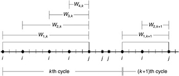
where n is the number of cycles and W1,k := Skj − Ski is the first passage time from state i to state j in the kth cycle (see Fig. 1).
[bull ] The overlapping estimator

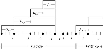
where n is again the number of cycles, Qk is the total number of visits to state i in the kth cycle, and Wl,k is the passage time from state i to state j for the lth visit of state i in the kth cycle (see Fig. 2 and the discussion that follows).

Overlapping passage time estimator in a Markov chain.

Structure of the overlapping estimator.
In order to clarify the structure of the overlapping estimator, note that each cycle begins with a visit to i and consists of a number of excursions from i during which the process returns to i without having visited j plus a final excursion starting from i and reaching j without returning to i. The last segment of each cycle is the return from j to i. During this last segment, the state j can appear several times, but the state i appears only at the end of the segment. The appearance of i signals the beginning of the next cycle. If we denote by Q the number of times that state i occurs during a typical cycle (note that we have dropped the subscript that refers to the cycle for simplicity), then we have Q − 1 excursions starting from i and ending at i that do not include state j plus a trip from i to j that does not return to i. Let us denote by U1,U2,…,UQ−1 the lengths of the Q − 1 excursions that return to i and by V the length of the final trip. Then, during this cycle, the overlapping estimator counts Q passage times from i to j, namely W1 = U1 + U2 + ··· + UQ−1 + V and W2 = U2 + ··· + UQ−1 + V,…,WQ = V. For instance, in Figure 2, Qk = 4, W1,k = U1,k + U2,k + U3,k + Vk, and W3,k = U3,k + Vk.
Clearly, because of the regenerative structure of this process, the resulting cycles are independent and identically distributed (i.i.d.) objects, and, in particular, the random variables Qk, k = 1,2,…, are i.i.d. Let

denote the probability that, starting from state i, we visit state j before we return to i, and let

denote the probability of the complementary event. Then it is clear by the strong Markov property that Q is a geometric random variable with probability of success p. Furthermore, also as a consequence of the strong Markov property, it follows that the successive excursion times from i to i without visiting j within a cycle, Ul, l = 1,2,…,Q − 1, are conditionally independent, given Q, with common distribution

which does not depend on Q. Finally, V is independent of {Q;U1,…,UQ−1} with distribution

From the above we obtain the following equivalent description of the structure of our regenerative cycles. We can assume that we have a sequence of i.i.d. random variables with distribution gii which we will designate by {Ul; l = 1,2,…}, a random variable V with distribution gij, and a geometric random variable (r.v.) Q with probability of success p. Furthermore, let {Ul}, V, and Q be independent. Then the collection of r.v.'s {Q;Ul,l = 1,2,…,Q − 1,V} describes the cycle completely.
We thus have

and, taking expectations,

Since Q is geometric, EQ = 1/p and E [Q − 1] = q/p, from which we obtain

We close the above discussion by noting that the overlapping estimator can also be written as

a fact that will be used in the sequel.
3. STRONG CONSISTENCY OF THE TWO ESTIMATORS FOR THE MEAN PASSAGE TIME IN MARKOV CHAINS
Recall that an estimator is strongly consistent if it converges with probability 1 to the quantity to be estimated as the number of observations goes to infinity.
Proposition 1: Both the simple and the overlapping estimator defined earlier are strongly consistent; that is, as n → ∞,

and

with

Proof: Equation (5) is an immediate consequence of the Strong Law of Large Numbers. (The irreducibility and positive recurrence of the Markov chain guarantee the finiteness of EW.) Thus, the simple estimator is clearly strongly consistent. The limit (6) is immediate if we divide both the numerator and denominator by the number of cycles n and appeal again to the Strong Law of Large Numbers. Thus, to establish the strong consistency of the overlapping estimator, it suffices to show (7). Indeed, the numerator on the left-hand side of (7) is

(where we have used the independence of {Ul}, V = UQ, and Q). Hence, the left-hand side of (7) becomes

Since the descending factorial moment of order m of the geometric distribution is given by

we easily see from (8) and (9) that

The above, together with (3), establishes (7) and, hence, the strong consistency of the overlapping estimator. █
Proposition 1 is established in Singh and Sutton [16] by means of a heuristic argument and in Bertsekas and Tsitsiklis [1]. It is included here for the sake of completeness of the discussion.
4. ASYMPTOTIC VARIANCE COMPARISON OF THE TWO ESTIMATORS
We now proceed to compare the two estimators in terms of their respective asymptotic variances. For the simple estimator, we have Var(Φn) = (1/n)Var(W) (due to the independence of cycles) and, hence,

Using the independence of {Ul}, V, and Q, we have

and since Q is geometrically distributed,

Thus, we conclude that the simple estimator is unbiased and its asymptotic variance constant is given by the above expression.
We now turn our attention to the overlapping estimator, which is a ratio estimator. We saw in Section 3 that it is strongly consistent. The following theorem (which is an adaptation of a classic result regarding asymptotic statistics; e.g., see Cramér [5, p.353] and Prakasa Rao [13, p.146]) shows that it is also asymptotically unbiased and gives its asymptotic variance.
Theorem 1 (Ratio estimator): Let (ξk,ζk), k = 1,2,…, be i.i.d. vectors such that, for some δ > 0, P(|ζ| > δ) = 1 and Eζ ≠ 0. We assume that both ξ and ζ have finite second moments. Then, as n → ∞, the ratio estimator

converges with probability 1 to

Furthermore, Rn is asymptotically unbiased and its bias is O(n−1); in fact,

Finally, the limit

exists and is given by the expression

The limit (13) is the asymptotic variance constant and it characterizes the behavior of the estimator when the number of cycles is large, since, in that case, Var(Rn) = (σ2/n) + o(1/n). Based on Theorem 1, and in view of the fact that MSE = (bias)2 + variance, we realize that the contribution of the bias term to the MSE is asymptotically negligible compared to that of the variance. Thus, we can ignore the bias term in our comparison of the two estimators.
We now turn our attention to the asymptotic variance of the two estimators.
Theorem 2: In any irreducible, positive recurrent Markov chain with countable state space, the simple estimator of the mean passage time for any pair of states i and j is superior to the overlapping estimator in terms of asymptotic variance and in fact it holds that the asymptotic variance ratio (AVR) is given by

where σΨ2 := limn→∞ n Var Ψn and q is given by (2).
Proof: Applying Theorem 1 (which guarantees the existence of σΨ) and taking into account Proposition 1, we obtain

with

In order to be able to compare directly the asymptotic variance constant of the overlapping estimator, σΨ2, with that of the simple one, given in (11), we need to express (16) in terms of p and the moments of U and V. Since Q is geometric, we have

The “covariance” term in (16) can also be easily computed taking into account the independence of Q, V, and {Ul} as follows:

Writing ½E [Q2(Q − 1)] = ½E [Q(Q − 1)(Q − 2)] + E [Q(Q − 1)] and using (9), we find

Finally,

Let us examine each of the three terms on the right-hand side of (20). For the first, we have

for the second,

and, finally, for the third,

The first term on the right-hand side of (23) is equal to

where we have used, once more, the expression for the descending factorial moments of the geometric distribution (9). The second term on the right-hand side of (23) is

Hence, from (20)–(25), we have

Thus, using (16)–(26), after carrying out the necessary simplifications we obtain the following expression for the asymptotic variance:

Comparing the above expression for the asymptotic variance constant of the overlapping estimator with that of the simple estimator, given in (11), we obtain (15). █
Thus, for the mean passage time estimation, the simple estimator is always superior to the overlapping one in terms of asymptotic variance, despite the fact that it might appear more wasteful. Although the overlapping estimator obtains more measurements over any given sample path than the simple estimator, these measurements are obviously strongly correlated. When q is close to zero (i.e., when returning to i before visiting j is very unlikely), the two estimators are essentially the same and their asymptotic variances are nearly equal. When, on the other hand, q is close to 1, then the overlapping estimator has asymptotic variance that is nearly twice that of the simple estimator.
We should point out that the above analysis is asymptotic and might not provide the complete picture if one is interested in the small sample behavior of the two estimators. In that case, one could use the mean squared error as a comparison criterion. For the simple estimator, which is unbiased, this is equal to Var(Φn). However, for the overlapping estimator, which is only asymptotically unbiased and whose variance was obtained asymptotically using Theorem 1, the situation is more complicated. Some results on this are provided in Singh and Sutton [16] and Bertsekas and Tsitsiklis [1, p.186].
5. ESTIMATING THE DISTRIBUTION OF THE PASSAGE TIME
Consider now the same problem where the object is to estimate the probability that the passage time exceeds a given threshold,

[i.e., the probability Pi(Tj > ν)]. Using the simple estimator, this is estimated by

whereas the overlapping estimator is given by

It will be convenient to use the notation

Also, as in the previous sections, in order to simplify the notation we will drop the subscript designating the cycle when not necessary. Thus, for instance, ξl can be used instead of ξl,k. Clearly, from the Strong Law of Large Numbers, Φn is a strongly consistent estimator of

Also, let

Then E [ξl|Q = m] = βm+1−l, where l = 1,2,…, m. Note in particular that

Finally, define the generating function

. Note in particular that

.
Theorem 3: With the above definition, we have the following:
(i) Ψn is also a strongly consistent estimator of r.
(ii) The AVR of the two estimators is given by

(iii) An alternative expression for the AVR is

where

.
Proof: By virtue of the Strong Law of Large Numbers, we have, as n → ∞,

The numerator of the right-hand side of (34) can be computed by conditioning on Q as follows:

the last equation following as a result of definitions (30) and (29). This, together with the fact that EQ = p−1, establishes the strong consistency of the overlapping estimator. Regarding the asymptotic variances, we first note that

On the other hand, the asymptotic variance of the overlapping estimator can be computed as in Section 4 by first computing EY2 and EYQ, where

. This is accomplished by first conditioning on Q, as follows:

In the above string of equalities, the third follows from the fact that ξl takes only the values zero and one and also from the fact that for l′ < l, {Wl > ν} ⊂ {Wl′ > ν} and, thus, ξlξl′ = ξl. Therefore, taking expectation with respect to Q in (36), we have

Also,

From Theorem 1 we have

where r = EY/EQ, EQ = 1/p, and EQ2 = (1 + q)/p2. Substituting the above into (38), we obtain

Thus, dividing the above expression by r(1 − r), we establish (32).
The alternative expression for AVR is obtained by straightforward algebraic manipulations, which we omit. █
In closing this section we should point out the significance of

in (33). It is obtained by averaging the βm's not with the geometric distribution with probability of success p (which is the distribution of Q) as in (31), but with a negative binomial distribution, which expresses the sum of two such geometric random variables. Since βm is increasing in m, as can be seen by its definition, it follows from a simple stochastic ordering argument that

and, hence, that

. Thus, we have

This should be compared with the corresponding equality (3) of Theorem 2. As we will see in Section 6 by means of an example, there are situations where AVR < 1, thus making the overlapping estimator more efficient than the simple estimator for large samples, unlike the situation where one tries to estimate the mean passage time.
Finally, we point out that the above results can readily be extended to continuous-time Markov chains and to Markov-renewal processes. Also, the target state j could easily be replaced by a set of states, J.
6. A TWO-STATE MARKOV CHAIN
To obtain more insight into this situation, consider a caricature of the problem we have examined, namely a discrete-time Markov chain with state space

and transition probability matrix

We want to estimate the mean passage time from zero to one, which, in this case, is a geometric random variable with probability of success p. Therefore, the variance constant for the simple estimator is

For the overlapping estimator we have

and the asymptotic variance constant is given by

Using again the expressions for the moments of the geometric distribution, we obtain, after some algebraic manipulations,

We see that the ratio of (40) to (41) satisfies (15).
However, it should be pointed out that although the overlapping estimator for the mean passage time is inefficient, the situation is different if the object is to estimate the distribution of the passage time. For instance, suppose that we are interested in the probability that the time required to make the transition from zero to one is strictly greater than ν. In this case, W1 = Q and

Also, βm = P(W1 > ν|Q = m) = 1(m ≥ ν + 1) and B(x) = (1 − x)−1xν+1. In that case straightforward algebraic manipulations give the following expression for the value of the AVR:

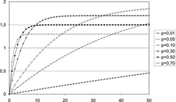
Figure 3 shows plots of the ratio as a function of ν for various values of p. As we can see, for small values of ν and small values of p, the value of the ratio in (42) is less than one and thus the overlapping estimator has a smaller asymptotic variance than the simple estimator.

Ratio of asymptotic variances for the two-state Markov chain as a function of ν for various values of p.