An essential component of the “Malthusian” model of pre-industrial society as now used by economists to model a society in which incomes are kept at subsistence levels by the interaction of fertility and land supply is that population growth, birth rates minus death rates, increased with income per person.1
See, for example, Miller and Upton, Macroeconomics, chapter 1; Galor and Weil, “Population”; Galor and Moav, “Natural Selection”; Hansen and Prescott, “Malthus”; Lucas “Industrial Revolution”; and Clark, Farewell. The modern Malthusian model does not necessarily conform exactly with what Malthus had in mind in any of the editions of his famous Essay, so the term “Malthusian” refers to just a general class of models.
Note that there will be different subsistence levels across different societies. In these modern Malthusian models the subsistence income is by definition the income at which the population is unchanging.

FIGURE 1 THE BASIC ASSUMPTION OF ALL MALTHUSIAN MODELS ON INCOME AND FERTILITY
However, empirical tests of this assumption for pre-industrial Europe and Japan have often detected only weak links between either mortality and real incomes, or fertility and real incomes.
The ideal data would be the fertility and mortality of cross sections of the population by income at a given time. But such studies for pre-industrial society are surprisingly few, and the results mixed. Parish register records of baptisms, burials, and marriages, which are the raw material of demographic enquiry for pre-industrial England have been largely mute on the issue of reproductive success and income or wealth, because of the difficulty of systematically linking family reconstitution records with those on the material and social circumstances of families. The extensive exploration of fertility and mortality by the Cambridge Group through reconstructing the family histories of a sample of 20 or so parishes, thus contents itself with looking at fertility and mortality by parish characteristics—agricultural, manufacturing, trading, mixed—as opposed to at the individual level.3
Wrigley et al., English Population History.
Landers, Death, pp. 186–88.
Hollingsworth, Demography, pp. 54–57; and Wrigley et al., English Population History, p. 614.
Zvi Razi finds evidence among the male property owners of medieval Halesowen of greater life expectancy among tenants of more substantial holdings in the period before the onset of the Black Death. Thus cottagers and small holders had a life expectancy of 20.8 years on taking up a holding, whereas the substantial tenants had a life expectancy of 33.3 years. But in the years 1350 to 1400 after the onset of the Black Death this differential disappeared, with small and large tenants having about the same life expectancy. And the very rich monks of Westminster Abbey in the later middle ages similarly display very low adult life expectancies.6
Razi, Life; and Harvey, Living.
In France more studies have linked family reconstitution studies for individual communities with records of occupation, literacy, and wealth. But earlier studies in this vein found little relationship, or even a positive relationship between wealth and infant mortality.7
See Derouet, “démographie”; and Charbonneau, Tourouvre cited in Weir, “Family Income,” p. 17.
Weir, “Family Income.” Bobbi Low found similar results for the Swedish parish of Tuna, but this was for the later nineteenth century. Low, “Occupational Status.”
Hadeishi, “Economic Well-Being.”
There were important variations in long-term real wages in the pre-industrial era. Real wages in England, for example, were at extraordinarily high levels in the fifteenth century and very low levels in the early fourteenth and seventeenth centuries. Life expectancy at birth does not seem to have been any higher in the high wage eras, certainly in the years 1538–1800.10
We can see this by comparing the life expectancies given in Wrigley et al., English Population History, p. 614, to real wages in this era from Clark, “Condition.”
Real income did vary dramatically from year to year in the pre-industrial world because of harvest failures. Many studies have thus examined the connection between annual grain prices and annual mortality rates. Here we would expect the short-run effects of income on fertility and mortality to be more muted than the long-run effects, because people have reserves they can draw on in the short run. Patrick Galloway summarized and updated these studies in a systematic fashion. In general the connection between grain price spikes and mortality rates is hard to detect, because of large variation in annual mortality rates caused by epidemic disease. It is largely absent in England after the 1540s. It was also absent in Japan.11
Tsuyo and Hamano, “Mortality.”
Galloway, “Basic Patterns,” p. 303.
Here we test the Malthusian assumption for a large cross section of the population in England circa 1600. The measure we use is the “reproductive success” of males aged 16 and above. We define that as the number of surviving children a man had at the time of his death, counting as surviving children also children who were dead but had themselves left surviving offspring. This measure will correlate highly with the net reproduction ratio for men.13
If all underage children were to live to 16, then this number divided by two would be the male version of the Net Reproduction Ratio.
WILLS AS A SOURCE FOR REPRODUCTIVE SUCCESS
The source of our information on both reproductive success and economic status is wills. These have been previously employed as an index of population growth only for the years before 1538 when parish registers began to be maintained on a regular basis. Robert Gottfried, for example, used wills as the main evidence for demographic trends in East Anglia in general, and Bury St. Edmunds in particular, in the years before 1538.14
Gottfried, Epidemic Disease and Bury St. Edmunds. Sylvia Thrupp seems to have been the one to first turn to this source. See Thrupp, “Problem.”
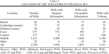
Here we use a sample of more than 2,000 wills by male testators in the years 1585–1638. These dates were chosen because of the existence of a number of printed sources summarizing comprehensive samples of wills in various locations for these years. The wills used are mainly from testators in East Anglia—Cambridge, Essex, and Suffolk—but include a group of wills from London (though for London without the asset information), as well as from two towns outside this region, Bristol and Darlington. Table 1 shows the composition of the sample by location, as well as the types of information available on economic and social status.

Despite the assumed Malthusian nature of the pre-industrial economy, English population in this interval grew at the moderate rate of about 0.56 percent per year. Thus E. A. Wrigley et al. estimate that from 1585 to 1838 the net reproduction ratio, the average number of daughters that would be born to a woman if she passed through her lifetime from birth conforming to the age-specific fertility and mortality rates of that era, was 1.21.15
Wrigley et al., English Population History, p. 614.
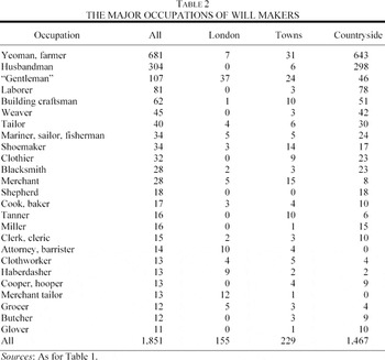
Wills were also not made by a random sample of the population, but were instead made by those who had property to bequeath. But the custom of making wills seems to have extended well down the social hierarchy, at least in East Anglia from where most of our wills were drawn. Table 2 shows the major occupations recorded. As the table implies, higher income individuals were undoubtedly more likely to make wills, but there are plenty of wills available for those at the bottom of the hierarchy such as laborers, sailors, shepherds, and husbandmen. Indeed we estimate that in Suffolk in the 1620s 39 percent of males who lived past age 16 made a will that was probated.16
Evans estimates that perhaps no more than 5 percent of the population at this time left wills (Evans, Wills … 1630–35). But we estimate 39 percent from the following calculation. In Suffolk male wills could be proved in one of four ecclesiastical courts: one of the two archdeaconry courts, the Norwich Consistory Court, or the Prerogative Court of the Archbishop of Canterbury. We know the male will totals per year in the archdeaconry courts (289), and in the Prerogative court (11). So adding a modest 11 for the missing court gives us 311 male wills per year. The population of males in Suffolk in the 1630s is estimated at 130,000: the population in 1801 scaled back to the 1620s by the national population totals. That implied a male population 16 or above of 65,000. We find below that the life expectancy of males making wills at age 16 was 39 years. So the number of male deaths per year in this potentially will making population would be 820. Thus 39 percent of males dying as adults made wills that were probated.

These wills were typically made close to the death of the deceased. The maximum time between the writing of the will and the death of the testator can be established by comparing the date of the will with the date probate was granted.17
Where a dated codicil was attached to a will, that date was taken as the date of composition of the will.
Wills were of two types. The majority were written wills, signed (or marked) by the testator. There were also “nuncupative” wills, which were statements of the testamentary wishes of the testator constructed by witnesses after the death. These wills were only included where they were detailed enough to include specific bequests.
The wills employed contain some or all of the following information: the occupation of the testator, the marital status (single, married, widowed, remarried), the number and genders of children, the literacy of the testator, all monies bequeathed, and to whom, the number of houses bequeathed, whether land was bequeathed (generally the amount of land was indicated in only about 20 percent of wills), and other goods bequeathed that have an ascertainable value (silver spoons, gold rings, horses, cattle, sheep, pigs, grains).19
Widowed was inferred from specific statements about former wife, or absence of wife in will when children were left bequests. Literacy was measured by whether the will was signed, the testator bequeathed books other than a bible, or the testator had an occupation requiring literacy such as an attorney or cleric.
Here is the summary of a typical will from Suffolk in 1623:
JOHN WISEMAN of Thorington, Carpenter (signed with X), 31 January 1623. To youngest son Thomas Wiseman, £15 paid by executrix when 22. Wife Joan to be executrix, and she to bring up said Thomas well and honestly in good order and education till he be 14, and then she is to bind him as apprentice. To eldest son John Wiseman, £5. To son Robert Wiseman, £5 when 22. To daughter Margery, £2, and to daughter Elizabeth, £2. To son Matthew Wiseman, £0.25. Rest of goods, ready money, bonds, and lease of house where testator dwells and lands belonging to go to wife Joan. Probate, 15 May 1623. 20
Allen, Wills, p. 266.
Wills of this period, unlike the wills of the fifteenth century investigated by Thrupp and Gottfried, seem to typically mention nearly all surviving children or their descendants.21
The wills investigated by Thrupp and Gottfried for the years 1412–1492 imply that throughout this period even the relatively advantaged group of testators with probated wills suffered catastrophic losses of one-third to two-thirds of the population each generation (Thrupp, “Problem,” table 2, p. 115; and Gottfried, Epidemic Disease).
Evans, Wills … 1636–38, p. 108.
Evans, Wills … 1636–38, p. 217.
Thus daughters were more likely to be omitted than sons. Hence the ratio of boys to girls named in wills can be used as one test of whether many children were being omitted. Also by looking at this ratio by the wealth or social status of testators we can test more importantly whether poor testators were more likely to omit children from their will.
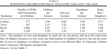
On the overall rate of omissions of children consider Table 3, which shows the number of children, and of sons and daughters mentioned in wills by the residence of the testator. The ratio of boys to girls overall would be about 1.05 at birth, 1.03 at ages one to 25, then switching towards a higher ratio of boys in the years 25 to 45 as women experience higher mortality from childrearing.24
Based on estimated relative male and female mortality rates by age in 1580–1649 (Wrigley et al., English Population History, pp. 296, 303).
Gottfried, Epidemic Disease, pp. 190, 198.

We use the ratio of boys to girls as one test of whether the omission rates varied by time period, social class, and the wealth of the testator. For each testator with at least one child we calculated the proportion which was boys (thus ranging from zero to one). Then we regressed this on various family characteristics—town location, literacy, estimated assets at death, occupation, and decade of the will—weighting by the number of children in the family. Every variable except one had no connection of any kind with the proportion of boys named: town residents, the literate, and those writing wills in later years all named the same proportion of boys to all children, 0.52. Most importantly for our purposes there was no significant connection, quantitatively or statistically, between the assets of the testator and the fraction of children who were boys. When we look at the strong positive association between assets and children below, there is no evidence that it is a product of girls being omitted from the wills of those with little to leave. When we look at social groups, only one of the seven showed any tendency towards more boys, and this was the lowest one, laborers. The proportion of boys in the wills of laborers averaged 60 percent, as opposed to 52 percent for the other groups, and despite the small size of this group this difference was big enough to be statistically significant. Because low assets and literacy, both aspects of the laborers as a social group, were not associated with fewer girls appearing in wills, this result is a little anomalous and is perhaps just the result of chance.26
These results are available on request.
It might be still possible that poor families, having little to leave, more often omitted both boys and girls equally, which our gender ratio test will not discover. We can control for this kind of gender neutral omission by also examining the relationship between wealth and the frequency of either no child being named as an heir, or of no male heir being named. The reasoning is as follows. Even if poorer testators omit some children from their wills because they have few assets, or chose to leave everything to one child, they will certainly not omit all their children for this reason. Further, given the preference for males as heirs, while they might leave assets only to the oldest son, they would not omit all their surviving sons from a will. Thus if we take as an index of fertility either just the frequency of at least one child being named, or the frequency of at least one son being mentioned in the will, this should be proof against the type of omission of children possibly to be found in poorer families. We shall see that when our analysis of fertility is carried out using these as alternative measures the results remain as strong as when using all children.
Because we are interested in the reproductive success of testators, dead children were counted as surviving offspring if they themselves had produced living offspring. Thus William Cooke of Great Livermere in Suffolk, who died at about age 74, left four living children, but also two dead sons who both had two surviving children.27
Evans, Wills … 1630–35, p. 359.
As can be seen in Table 3 the average numbers of children per testator were modest. For a population to be just reproducing itself the numbers of children surviving each male at time of death would have to exceed two. It has to exceed two because some of these children are minors who would die before they would reach the age (sixteen or more) where they would be potentially writing wills. We describe below how we link a subsample of the testators to parish records. This enables us to estimate the age distribution of the surviving children, for 379 children. Thirty-three percent of these surviving children were below age 16. Applying the mortality estimates for the general population derived by Wrigley et al. to this age distribution we estimate that for the average testator to get two children who survived to age 16 at least they would need to leave 2.07 children when they died.28
The survival rates used were from Wrigley et al., English Population History, p. 215.
ESTIMATING ECONOMIC STATUS
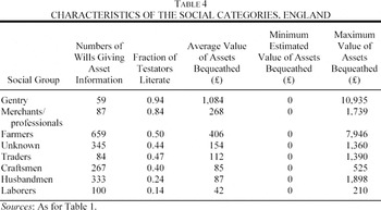
From the information in the wills we can estimate the economic status of the testator in two ways. The first is from the occupation ascribed to the testator. The second is from estimating the value of assets bequeathed. To simplify the occupation structure somewhat we organized male testators into the seven social categories shown in Table 4. As can be seen these categories as a whole correlate well with two other measures of social status, literacy and assets bequeathed (derived below). Thus these occupations alone explain 18 percent of the variation in income. But within each social group there are wide variations in the economic position of the testator. There were laborers as rich as the average craftsman or trader, and craftsmen as rich as the average merchant, cleric, or attorney. Many husbandmen were richer than the average yeoman. Similarly, some laborers were literate, and many yeomen illiterate. So the social labels given in the wills are loose.

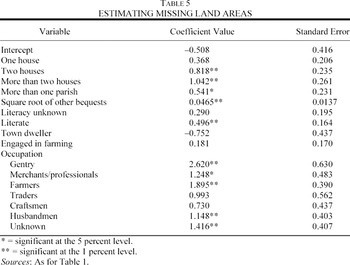
The estimated assets of testators were constructed from the information in wills by adding together the cash payments directed by the testator, with the estimated value of houses, land, animals, and grain bequeathed by the testator. Although land was bequeathed in 975 of the wills in our sample, in only 209 cases, one in five, was the area of the land indicated. To infer the area in the other 766 cases, we estimated for the observed cases area as a function of other features of the will: the number of houses bequeathed, the number of additional parishes the land was described as lying in, the total amount of cash and goods bequeathed, an indicator for the literacy of the testator, an indicator for whether the testator lived in a town, an indicator of whether the person engaged in farming, and indicators for each occupational group. The functional form that best fit the observed cases was chosen by experiment. Thus the estimated expression was

where HOUSE1 was an indicator set to one if one house was bequeathed, HOUSE2 an indicator for two houses, HOUSE3 an indicator for three or more houses, MOREPAR an indicator for land left in more than one parish, BEQROOT the square root of the value of cash and stock bequeathed, DLIT an indictor for a literate testator, DLITUNKNOWN an indicator for someone whose literacy is unknown, DTOWN an indicator for a town dweller, DFARMER an indicator for someone engaged in farming, and OCCUPi indicators for the six occupational groups defined previously other than laborers. DFARMER was set to one if the testator left farm animals or grain in the will, or left farm implements. To normalize for changes in the price level over the years 1585–1836 the BEQROOT variable in the equation was constructed using the actual cash bequests in the will normalized by the average price level in each of the decades 1580–1589, 1590–1599, 1600–1609, 1610–1619, 1620–1629, and 1630–1639. To this was added the value of the stock left calculated using a standard set of values normalized to the 1630s: horses £5, cattle £4, sheep £0.5, pigs £2, wheat (bu.) £0.21, barley/malt (bu.) £0.10, oats (bu.) £0.07, peas/beans (bu.) £0.12, silver spoons £0.375, gold rings £1.
Table 5 shows the estimated coefficients and their statistical significance. Most of the statistically significant associations are in the direction we would expect. People leaving more houses and cash leave more land, as do literate people, people engaged in farming, and people of higher occupational status such as gentry, farmers, and merchants. The 2 is 0.512, which means that we explain more than half of all the variation in reported land areas with the reported characteristics. The areas of land actually observed ranged from 0.25 to 235 acres. The areas imputed ranged from 0.9 to 653 acres. The imputation of areas will thus be extremely noisy for cases where the area imputed is greater than 200 acres. But since any imputation of area of above 100 acres puts the person in our top income class we think this is not a major problem.

We then constructed a monetary measure of the wealth bequeathed by the testator at the time of death by adding to the value of the money and stock bequeathed an estimated value for houses (£40 each) and for land (£10 per acre).
29The house values are from Clark, “Shelter,” and the land values are from Clark, “Farmland.” We are aware that houses in country parishes were worth less than those in towns, but felt that not too much distortion was introduced by simply having a common value for all housing.

For male testators for whom we have enough information to estimate assets bequeathed, the average value of assets equaled £235 in 1630s prices (1.1 houses (£44), 9.9 acres of land (£99), £88 in cash bequests (in the prices of 1630–1639) and £4 in stock). But the median value was only £99.8. This would generate an annual income of about £6 at the return on capital typical of this period. The yearly earnings of a carpenter in this period would be about £18, and of a laborer £12.
30See Clark, “Land Hunger,” for the rates of return. Clark, “Condition,” gives the wage rates.
One problem with this method of estimating the total bequest is that often the cash payments to children were to be paid by those who got the real assets, so rather than being in addition to the real assets they were a charge on them. But instead of trying to distinguish cases where the cash was an addition to real assets listed, rather than just a charge on these assets, we took the view that a true index of the wealth of the testator was likely to be more accurately revealed by the sum of these four components. Where more cash is charged against real assets the greater are these real assets likely to be.
ECONOMIC STATUS AND REPRODUCTIVE SUCCESS
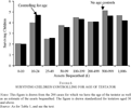
Were the numbers of surviving children linked to the likely income of the person in these years? We sorted males with information on bequests into eight asset classes: £0–9, £10–24, £25–49, £50–99, £100–199, £200–499, £500–999, and £1,000 and above. The class sizes were chosen in part to distribute the testators approximately equally between the classes.31
The shares in each class were 0.16, 0.08, 0.11, 0.15, 0.18, 0.19, 0.09, and 0.04 respectively.
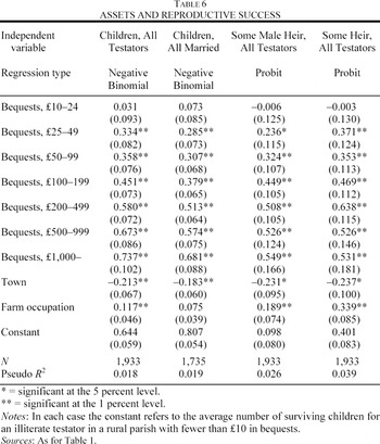
Table 6 shows the estimated association between assets and surviving children for all testators, and restricted to testators married at least once. Controls are included for town residence, and for the testators whose will revealed that they actually engaged in farming (by leaving grain, farm animals, or farm implements to their children). The estimate is done with a negative binomial regression because the number of children per testator is a count variable, but with over dispersion compared to the Poisson distribution.32
See Cameron and Trivedi, Regression Analysis, p. 70.

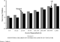
Figure 2 shows the estimated numbers of children per male of each bequest class for England as a whole outside London as revealed by the wills. For all married men, someone with less than £10 in bequests would typically have fewer than two children, whereas someone with £1,000 or more, nearly four children. As Table 6 and Figure 2 shows the link between assets and surviving children is extremely strong both statistically and quantitatively. If we instead estimate the link parametrically using the square root of assets as the independent variable, because the link between assets and reproductive success is nonlinear, we get a similar quantitatively and statistically strong coefficient on the square root of assets.33
We cannot use the more flexible measure of the log of assets as the independent variable because some testators have bequests with zero estimated value (such as clothing, kitchen utensils, work tools).

FIGURE 2 SURVIVING CHILDREN BY ESTIMATED ASSETS OF TESTATOR
The link shown here between assets and surviving children cannot be an artifact created by poorer testators omitting some children because they had nothing to bequeath them. This is evident in a number of ways. First we know from the work of Wrigley and his associates that the typical male testator in England in these years would leave 2.58 surviving children.34
Wrigley et al., English Population History, p. 614.
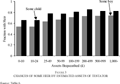
But we can also see from the evidence of the wills themselves that omission of children by poorer testators cannot explain the result. The fourth column of Table 6 shows the results for estimating (using probit) the likelihood that a testator left at least one son as a function of assets. There is again a strong link quantitatively and statistically. Only 54 percent of the poorest testators would leave a son, as compared to 74 percent of the richest. Figure 3 shows the percentage of testators with a son at each income class. Testators who omitted some children because of insufficiency of assets for bequests would not omit all their sons. Thus if the family size was really the same across rich and poor, the frequency of one son at least appearing in the will should be the same. Clearly it is not. Indeed for the actual distribution of sons across the 619 testators in the top three classes, we can calculate what would happen to the likelihood that a testator had no son if we just randomly removed half of these sons. The answer is that it drops from an observed 74 percent with a son to 56 percent, close to what we observe for the poorest testators. Thus the data here support the idea that the problem is not one that “excess” sons and daughters were not reported by poorer testators.

FIGURE 3 CHANCES OF SOME HEIR BY ESTIMATED ASSETS OF TESTATOR
The last column of Table 6 reports a similar exercise where we estimated the likelihood that the testator left any heir. Again if net fertility was constant across asset classes, but some children were omitted from the wills of poorer people, this frequency should also be constant across assets classes. Clearly it is not, and again the observed frequency of no heir at the lowest asset level can be predicted closely from the distribution of family sizes at the upper asset classes, just randomly deleting half the children. So the powerful link between assets and numbers of surviving children has nothing to do with some children being omitted from the wills of the poorer testators. We shall also see that it has nothing to do with assets proxying for age either.
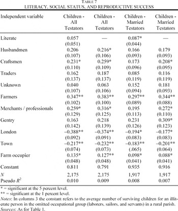
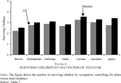
Assets predict reproductive success much better than do our alternative measures of income, which are occupation and literacy. Table 7 shows the estimated coefficients of a negative binomial regression of the numbers of children on literacy and occupational status, controlling again for residence and farming activity by testators. This sample includes also testators in London, so there is a control included also for London residence. The higher social classes do appear to produce more surviving children, but the effect is much weaker than for assets, both statistically and quantitatively. Figure 4 shows the numbers of surviving children by these broad occupational classes, controlling just for residency, as inferred from the negative binomial regression. Testators from the top three social groups produce on average three surviving children compared to 2.2 for laborers. But those described as “gentleman” or “esquire” are not particularly successful in reproduction, perhaps because in this case the term was used for younger people from the upper classes before they acquired an occupation (which would account for the greater proportion of gentry unmarried).


FIGURE 4 SURVIVING CHILDREN BY OCCUPATION OF TESTATOR
If we run a regression with assets, literacy, and occupation, both literacy and occupation become both quantitatively and statistically insignificant predictors of net fertility. It seems that only because occupation and literacy are indicators of assets do they on their own also explain reproductive success. Economic status rather than social class is what mattered for reproductive success in England in these years. Presumably this is because the occupational labels used to form people into status classes are imprecise. There were husbandmen who were literate and wealthier than yeomen who were illiterate. There were carpenters who worked for others and owned no assets, and there were carpenters who were employers and engaged in building and leasing property.
AGE, ASSETS AND SURVIVING CHILDREN
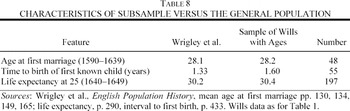
The strong positive association of bequeathed assets with numbers of surviving children might be explained by assets proxying for the age of the testator, if assets were steadily accumulated over the course of men's lives. But we can rule out this possibility using a subgroup of testators in our sample: those whose ages we can establish. We were able to get an estimate of age at time of making the will for 208 of the testators. We did this from one of four sources of information. First from the age being given in the will (2), second from a parish register baptism record (91), third from a parish register marriage record (77), and last is from a parish record baptism record for their oldest known child (38). We infer age from the date of the first marriage using the average age at the first marriage of the 48 testators where we know both baptism and marriage dates. The average age of first marriage for testators was 28.17 years. We infer age from the birth of the first child using the information supplied by 55 cases where we have the marriage date and the date of birth of the oldest child in the will. The average time between marriage and the birth of the first known child was 1.60 years. So in the 37 cases where only the date of birth of the oldest child was known we thus assumed that the testator was born 29.77 years before.35
To locate these testators in any reasonable length of time we had to use a secondary source, transcriptions of birth and marriage information from parish registers in the International Genealogical Index maintained by the Church of Jesus Christ of the Latter Day Saints. This site had a number of inaccuracies. Events in the early months of the calendar year, for example, were often incorrectly ascribed to the previous year, because the transcriber did not realize that the ecclesiastical year did not coincide with the calendar year.
The data on this subsample whose details can be located in parish registers can be used as a test of how representative our testators are of the general population in these years. Table 8 shows various characteristics of the life experience of our testators with the general population at this time as calculated by Wrigley and his associates. The average age at first marriage and average life expectancy at age 25 are very similar to those of the general population. The length of time between marriage and the Christening of the first child is a bit longer than the 1.33 years Wrigley et al. would suggest. But in our case the matching method used misses some earlier born children who died before the will, but either did not appear in the parish baptism register, or were not located because they had a first name other than that of the surviving children or of the parents.36
In other cases we found the date of such earlier births by looking for an earlier child with the same first names as the testator or his then wife, as first children tended to be named after the parents.

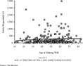
When we compare the ages of this subgroup of testators with their estimated assets at time of death we find the pattern shown in Figure 5. Though the ages of the 208 testators varied from 16 to 88, there is little connection between age at making the will and the value of the assets bequeathed. Thus when we regress ASSETS on AGE there is no significant upwards trend with age, and the fit is extremely weak.

FIGURE 5 AGE AT WRITING OF WILL AND ASSETS BEQUEATHED

with the standard error in parenthesis. Age explains only 1 percent of the variation in assets, so that if assets are highly correlated with net fertility, it cannot be through assets proxying for age.
Even if we allow for an inverse U shape in assets, as would be predicted by economic theory on the assumption that part of asset holding is to provide income by dissaving in old age, we still find a very poor fit. Regressing now assets on AGE and age squared (AGE2) we get

This is shown in the figure as the solid line. The coefficients on AGE and AGE2 are very imprecisely estimated, so that the exact shape of the relationship is unknown. The extremely low R2 shows that only 1 percent of the observed variation in assets can be explained by life cycle accumulation behavior.
These results are completely consistent with other studies of wealth by age in the pre-industrial era and the nineteenth century. Weir, in a study of 47 households in Rosny-Sous-Bois in 1747, also finds that age explains a tiny fraction of the variation in assets or incomes.37
Weir, “Family Income,” p. 11.
Lindert, “Luncrens Angliae.”
For the 200 testators for whom we have the size of the bequest and the number of children, we estimated the effect of assets on the numbers of children controlling for the age of the testator. To do this we included indicator variables for testators being aged zero to 29, 30 to 39, 40 to 49, and 50 and above at the time of writing the will. The age variables were important quantitatively and statistically in explaining the numbers of children. But, as would be expected from the foregoing discussion, controlling for age did not eliminate, or even much reduce, the under-lying relationship between assets and numbers of surviving children. Figure 6 shows the relationship between assets and children for this reduced sample both uncontrolled and controlling for the age of the testator. The small sample of 200 testators, and the large range of numbers of surviving children, from zero to 13 children, means that the relationship between assets and surviving children is not as smooth as for the larger sample. But it is still clearly there.

FIGURE 6 SURVIVING CHILDREN CONTROLLING FOR AGE OF TESTATOR
WHY DID RICHER MEN LEAVE MORE DESCENDANTS?
Richer married men could have left more children for any of a number of reasons. They may have married earlier, and so have survived longer to have children. They may have married younger wives. They may have been more likely to remarry if their wife died. They may have had more births per year of marriage, or these children might have survived better. The information from the wills, and from the group that can be linked to parish registers, allows us to narrow down these possibilities to only two. Either richer testators produce more children per year of marriage, or the children they produced survived better.
First, for the 68 cases in the subsample where we have both the birth date and at least an estimate of the marriage date there is no sign that the richer half of the testators married any earlier. The estimated age at marriage was the same for both groups. The 95 percent confidence interval for the difference in marriage age between richer and poorer is −2.7 years to +2.7 years (on an average of 27.6 years). Any difference in ages at marriage was thus likely to have been small.
Second, based on 180 cases the number of years married averaged 27.8 for the poorer and 29.1 for richer testators (with the 95 percent confidence interval on the difference being −3.0 years to +5.2 years). Thus again life expectancy differences were likely to be small between rich and poor, though the great variance of age at death makes this hard to estimate without a very large sample.
Third, probabilities of ever marrying were possibly, but only possibly, higher for richer men. Dividing the sample into those with less than £100 in bequests, compared to those with more than £100, we find that for 12.4 percent of poorer testators there was no evidence of any marriage, whereas this was true for only 7.7 percent of richer testators. However, the appearance that poorer men may be less likely to ever marry may be an artifact of the nature of the wills evidence. Some class of those identified as single will be widowers who had no children and whose will gave no evidence of their pre-deceased wives existence (though leaving bequests to her relatives, for example). Given the association between assets and reproductive success, these unidentified widowers will tend to be in the lower half of the asset distribution. Thus the data here overstate the difference in marriage frequency between rich and poor. Even if these data reflected true underlying marriage probabilities, the amount of the higher fertility of the rich this would explain is small—about 5 percent of the difference in numbers of surviving children.
Thus the greater reproductive success of richer men lay predominantly in the fact that they produced more surviving offspring per year of marriage, measuring that to the year of first marriage. That could come from some or all of three different sources: they may have married younger brides, they may have remarried at higher rates if their first wife died, or their children may have survived infancy and childhood better. We suspect, consistent with the evidence presented above on infant mortality across London parishes of different average wealth, that differential survival of children was the key. But the wills as a source are poor at revealing the existence of wives who died earlier when the testator has remarried, or when he was actually a widower but had no surviving children. Thus it is impossible to tell whether richer testators more frequently remarried.
THE SOCIAL CONSEQUENCES OF SURVIVAL OF THE RICHEST
England in the years 1585–1638 was still a relatively static society, with little change in income per person. It was, as noted, a society still in the Malthusian grip where economic change was slow or nonexistent. Consequently, the relative numbers of occupations, the wage rates for different occupations, and the stock of housing per person changed little. Land per person fell, but land values were increasing with the growth of population, so the value of land per person also changed little. The great reproductive success of richer testators thus meant that their children had to be on average moving down the social ladder in terms of assets and occupations, and moving down reasonably rapidly.
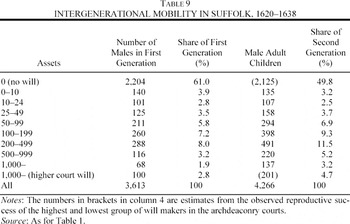
We illustrate this in Table 9 for Suffolk in the 1620s and 1630s. The second column of the table shows the sample of male will makers from Suffolk arranged by asset class. Added to the observed wills are the appropriately sized group of males who made no will, assumed to have no assets, as well an appropriately sized group of testators whose wills were approved in higher courts, and whose assets are assumed to all exceed £1,000. The next column shows the share of each class of males in the population in the first generation. The next column gives the observed numbers of male children from each asset class in Suffolk, reduced by 3 percent to allow for childhood mortality. This is the number of males who reach at least age 16 from each asset class. We assume the non-will makers had the same numbers of children as those making wills whose assets were less than £10. For those whose wills were proved in higher courts we assume they had the same numbers of children as those of the highest observed asset class. This implies that of a population of 3,613 wills in the first generation we end up with 4,266 adult male successors in the next generation, an increase of 18 percent per generation. This is very close to the gain of 21 percent per generation implied by the aggregate estimates of Wrigley et al. for England in this period.

The last column of the table shows the shares of the children of each asset class in the next generation. Testators with less than £10 in assets and those who left no will were 65 percent of the first generation. But their sons constituted only 53 percent of the next generation. Testators with more than £500 in assets were 7.9 percent of the initial generation. Their sons were 13.1 percent of the next generation. Given that assets per person in the population probably stayed constant over this interval, there thus must have been considerable net downward mobility in the population. Nearly half of the sons of higher class testators would end up in a lower asset class at death. Indeed net mobility would be downward for testators in all the groups with £25 or more in assets.
OTHER TIMES, OTHER PLACES
There are few published studies of the link between income and net fertility in the pre-industrial era. There is, however, evidence that the pattern uncovered here of much higher net fertility by richer groups existed in England at least by 1250. The King had a financial interest in the deaths of his tenants in chief, those who held land directly from him in the feudal system. These individuals were mostly an economically privileged group and included the highest nobility of the land. There were customary payments to the crown upon a succession, if the heir was under age it created a profitable guardianship for the crown, and if the heir was an unmarried female the marriage of the heiress might be in the hands of the king. Thus, from 1250 on, the King's officials conducted Inquisitions Post Mortem (IPM) on the deaths of these tenants, which are preserved in the Public Record Office. These inquisitions record only the following information, however, about surviving children: the oldest surviving son (or his descendants), failing a male heir all daughters (or their descendants), and failing any surviving child (or their descendants) the next of kin.
Josiah Cox Russell in a famous, and very ingenious, study, which in part inspired this article, used the information from the inquisitions from 1250 to 1500 to estimate the number of surviving offspring by quinquennia, and thus trends in English medieval population.39
Russell, British Medieval Population.
Russell, aware of this problem of too few women being reported, concludes improbably that “such a condition would probably have been the result of a systematic elimination of females at birth.” (Russell, British Medieval Population, p. 238).
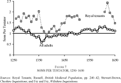
However, the evidence of the wills in 1585–1638 provides an alternative way to infer total numbers of surviving children from measures such as the fraction of times there was an heir, or the fraction of times there was a male heir, for wealthy groups such as royal tenants before 1500. Figure 7 shows two series by decade for England from 1250 to 1649. The first is the average number of males per adult inferred for the whole population of England from data on the aggregate movement of population. As can be seen, before 1500, except for the phase of population growth up to 1315, this number was one or below one. The second is the implied average number of adult male children produced by royal tenants. This was calculated by using the proportions revealed for 1585–1638 between total male surviving children and the fraction of testators leaving a son or leaving some child.

FIGURE 7 SONS PER TESTATOR, 1250–1650
In the two periods in medieval England where the population was stable or growing, 1250–1349, and 1450–1500 tenants in chief were producing on average about 1.8 surviving sons, nearly double the population average. Even in the years of population decline from 1350 to 1450, though implied surviving sons per tenant in chief declined, it remained at above the replacement rate in most decades. The gap between the net fertility of this rich group and the general population did, however, decline in these 100 years. As calibration, note that by the seventeenth century the royal tenants still showed replacement rates well above the general population, and rates similar to the wealthiest groups in our will sample.
Thus, as later in medieval England, the rich seem to have been out reproducing the poor, and again social mobility must have been generally in a downwards direction.
This story of the reproductive advantage of the rich is also found in a collection of surveys of communicants in villages in Austria and southern Germany for the seventeenth to nineteenth centuries assembled by Joerg Baten. Villagers of higher social status, and those revealed to be more likely literate had at the time of the surveys more surviving children.41
Joerg Baten, personal communication.
However, the reproductive advantage of the rich is not found in all pre-industrial societies. In a companion study to this one we have also looked at the reproductive success of French Canadians in the seventeenth and eighteenth centuries.42
Hamilton and Clark, “Economic Status.”
The authors thank David Brown and David Nystrom for excellent research assistance, and Oded Galor and Omer Moav for the original hypothesis that sparked this study. They thank also Joerg Baten, Peter Lindert, Kevin Salyer, Knick Harley (the editor), and two anonymous referees for advice and helpful comments. Clark acknowledges the research support of the National Science Foundation (grant SES 02-41376). Hamilton acknowledges the research support of the SSHRCC (Grant #41020020154).