1 Introduction
Diapycnal mixing, or the molecular diffusion of density across isopycnal surfaces, is a primary control on the ocean stratification (Munk & Wunsch Reference Munk and Wunsch1998; Wunsch & Ferrari Reference Wunsch and Ferrari2004). Turbulent stirring enhances this mixing by deforming isopycnal surfaces, creating both sharper density gradients and a greater surface area over which molecular diffusion can occur. Turbulent stirring is reversible, and represents an exchange between turbulent kinetic energy and available potential energy. Diapycnal mixing, however, is irreversible; it represents a sink of turbulent kinetic energy into the background potential energy of the fluid. Due to difficulties associated with measuring the turbulent fluxes that lead to diapycnal mixing in the ocean (see, e.g., Ivey, Winters & Koseff Reference Ivey, Winters and Koseff2008; Venayagamoorthy & Koseff Reference Venayagamoorthy and Koseff2016), a great deal of work has gone into estimating mixing using indirect methods. Such methods typically rely on directly measured quantities such as the turbulent kinetic energy dissipation rate
 $\unicode[STIX]{x1D716}$
or the temperature variance dissipation rate
 $\unicode[STIX]{x1D712}$
.
As outlined by Ivey et al. (Reference Ivey, Winters and Koseff2008), there are two common approaches for indirectly estimating turbulent mixing in the ocean. The first is the model of Osborn (Reference Osborn1980), which is based on measurements of
 $\unicode[STIX]{x1D716}$
, and approximates the turbulent diffusivity of density with
 $$\begin{eqnarray}K_{\unicode[STIX]{x1D70C}}=\left(\frac{R_{f}}{1-R_{f}}\right)\frac{\unicode[STIX]{x1D716}}{N^{2}}=\unicode[STIX]{x1D6E4}\frac{\unicode[STIX]{x1D716}}{N^{2}},\end{eqnarray}$$
where
 $N$
is the buoyancy frequency. The model also depends on the flux Richardson number
 $R_{f}={\mathcal{B}}/{\mathcal{P}}$
, where
 ${\mathcal{B}}$
is the turbulent buoyancy flux and
 ${\mathcal{P}}$
is the rate of production of turbulent kinetic energy. Following Ivey & Imberger (Reference Ivey and Imberger1991), the flux Richardson number is sometimes defined more generally as
 $R_{f}={\mathcal{B}}/({\mathcal{B}}+\unicode[STIX]{x1D716})$
. The term
 $\unicode[STIX]{x1D6E4}=R_{f}/(1-R_{f})$
is referred to as the mixing efficiency and represents the ratio of the turbulent buoyancy flux to the turbulent dissipation. The second commonly used mixing model is that of Osborn & Cox (Reference Osborn and Cox1972), which is based on measurements of
 $\unicode[STIX]{x1D712}=2\unicode[STIX]{x1D705}_{\unicode[STIX]{x1D703}}\overline{|\unicode[STIX]{x1D735}\unicode[STIX]{x1D703}^{\prime }|^{2}}$
, where
 $\unicode[STIX]{x1D703}^{\prime }$
is the temperature fluctuation from the background temperature
 $\overline{\unicode[STIX]{x1D703}}$
and
 $\unicode[STIX]{x1D705}_{\unicode[STIX]{x1D703}}$
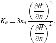
is the molecular diffusivity of heat. Using this model, the turbulent diffusivity of heat is given by
 $$\begin{eqnarray}K_{\unicode[STIX]{x1D703}}=3\unicode[STIX]{x1D705}_{\unicode[STIX]{x1D703}}\frac{\overline{\left({\displaystyle \frac{\unicode[STIX]{x2202}\unicode[STIX]{x1D703}^{\prime }}{\unicode[STIX]{x2202}n}}\right)^{2}}}{\left({\displaystyle \frac{\unicode[STIX]{x2202}\overline{\unicode[STIX]{x1D703}}}{\unicode[STIX]{x2202}n}}\right)^{2}},\end{eqnarray}$$
where
 $n$
is normal to isothermal surfaces, but in the field is always assumed to be the vertical direction
 $z$
(Ivey et al.
Reference Ivey, Winters and Koseff2008).
Based on their derivations from the turbulent kinetic energy equation and the temperature variance equation respectively, both the Osborn & Cox (Reference Osborn and Cox1972) model and the Osborn (Reference Osborn1980) model rely on a fundamental assumption that the flow is steady and homogeneous. However, this assumption is often violated in the ocean due to the intermittent (unsteady) and patchy (inhomogeneous) nature of ocean turbulence (Ivey et al. Reference Ivey, Winters and Koseff2008). Many studies have therefore related mixing to certain non-dimensional numbers, such as the turbulent Froude number and turbulent Reynolds number, that describe the state of the turbulence that leads to mixing (e.g. Ivey & Imberger Reference Ivey and Imberger1991; Mater & Venayagamoorthy Reference Mater and Venayagamoorthy2014a ).
Additionally, both the Osborn & Cox (Reference Osborn and Cox1972) model and the Osborn (Reference Osborn1980) model rely on a more implicit assumption which has received less attention in the literature: the stratification (
 $N$
in Osborn Reference Osborn1980;
 $\unicode[STIX]{x2202}\overline{\unicode[STIX]{x1D703}}/\unicode[STIX]{x2202}n$
in Osborn & Cox Reference Osborn and Cox1972) is assumed to represent the background gradient against which turbulence must work to stir the fluid. The background stratification is typically well defined in idealized numerical models, which have been used extensively to study turbulent mixing. For example, it can be held constant (e.g., Shih et al.
Reference Shih, Koseff, Ivey and Ferziger2005) or it can be obtained through an adiabatic rearrangement of the full three-dimensional density field (Winters et al.
Reference Winters, Lombard, Riley and D’Asaro1995; Scotti & White Reference Scotti and White2014). However, the appropriate background stratification is much less obvious in the ocean, and even to some extent in the laboratory (e.g. Hult, Troy & Koseff Reference Hult, Troy and Koseff2011).
Due to practical limitations in the ocean, turbulence data are almost always gathered using vertical-profiling instruments. Thus, when the Osborn & Cox (Reference Osborn and Cox1972) and Osborn (Reference Osborn1980) models are used in the field, the background stratification is estimated through adiabatic rearrangement, or sorting, of one-dimensional vertical density profiles. This practice began with the study of Thorpe (Reference Thorpe1977), continued with Dillon (Reference Dillon1982), and is still very common today (see, e.g., Thorpe Reference Thorpe2005; Ivey et al. Reference Ivey, Winters and Koseff2008). Due to the intermittent patchy nature of turbulence in the ocean, it is unclear how well this estimated background stratification represents the true stratification against which turbulence is working. Any differences between the background stratification calculated using this methodology and the true background stratification will translate to errors in estimates of turbulent mixing.
In this study, the discrepancy in estimates of turbulent mixing that arises from the chosen calculation of the background stratification is quantified in the context of breaking internal waves on slopes. Particular attention is paid to the flux Richardson number
 $R_{f}$
, which must be determined in order to estimate mixing from measurements of
 $\unicode[STIX]{x1D716}$
and
 $N$
using the Osborn (Reference Osborn1980) model. While Osborn (Reference Osborn1980) originally assumed a constant
 $R_{f}\approx 0.17$
, many parameterizations have been developed to estimate
 $R_{f}$
based on the state of the turbulence (e.g. Ivey & Imberger Reference Ivey and Imberger1991; Shih et al.
Reference Shih, Koseff, Ivey and Ferziger2005; Bouffard & Boegman Reference Bouffard and Boegman2013). Due to the difficulties in calculating
 $R_{f}$
in unsteady inhomogeneous turbulence in the field, these parameterizations are generally based on the results of idealized laboratory experiments and direct numerical simulations (DNS). Several field studies that have measured the turbulent buoyancy flux directly (e.g. Davis & Monismith Reference Davis and Monismith2011; Walter et al.
Reference Walter, Squibb, Woodson, Koseff and Monismith2014) have shown good agreement with existing parameterizations. The study of Mater & Venayagamoorthy (Reference Mater and Venayagamoorthy2014b
) provides a thorough summary of the current state of
 $R_{f}$
parameterizations in the literature. However, the existence of a ‘universal’ parameterization for
 $R_{f}$
remains an open question.
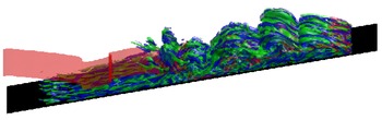
The effect of the background stratification on the resulting mixing calculation is quantified using the DNS dataset of Arthur, Koseff & Fringer (Reference Arthur, Koseff and Fringer2017). As highlighted in figure 1, breaking internal waves on slopes are an inherently unsteady inhomogeneous flow, and are thus a useful case study for calculating and interpreting
 $R_{f}$
. By varying the calculation of
 $N$
, it is shown that the chosen method can affect not only
 $R_{f}$
, but also the values of the non-dimensional parameters upon which
 $R_{f}$
depends.
A three-dimensional view of the turbulent flow field during breaking for an internal wave with intermediate interface thickness (case 5 in Arthur et al.
Reference Arthur, Koseff and Fringer2017). Isosurfaces of the reference density
 $\unicode[STIX]{x1D70C}=\unicode[STIX]{x1D70C}_{0}$
(red), positive streamwise vorticity
 $\unicode[STIX]{x1D6FA}_{1}/\unicode[STIX]{x1D714}=37$
(blue) and negative streamwise vorticity
 $\unicode[STIX]{x1D6FA}_{1}/\unicode[STIX]{x1D714}=-37$
(green) are shown, where
 $\unicode[STIX]{x1D714}$
is the frequency of the incoming wave.

2 Methods
The DNS dataset of Arthur et al. (Reference Arthur, Koseff and Fringer2017) includes results from eight breaking wave cases with varying interface thickness (and thus varying stratification), but with similar incoming wave properties. From these data, turbulent dissipation and irreversible mixing quantities are calculated as follows. Turbulent dissipation is defined as
 $$\begin{eqnarray}\unicode[STIX]{x1D716}_{k}^{t}=2\unicode[STIX]{x1D708}\overline{\unicode[STIX]{x1D61A}_{ij}^{\prime }\unicode[STIX]{x1D61A}_{ij}^{\prime }},\end{eqnarray}$$
where
 $\unicode[STIX]{x1D708}$
is the kinematic viscosity and
 $\unicode[STIX]{x1D61A}_{ij}^{\prime }=((\unicode[STIX]{x2202}u_{i}^{\prime }/\unicode[STIX]{x2202}x_{j})+(\unicode[STIX]{x2202}u_{j}^{\prime }/\unicode[STIX]{x2202}x_{i}))/2$
is the turbulent rate-of-strain tensor. Irreversible turbulent mixing is defined generally as
 $$\begin{eqnarray}\unicode[STIX]{x1D716}_{p}^{t}=\unicode[STIX]{x1D705}\frac{\overline{|\unicode[STIX]{x1D735}b^{\prime }|^{2}}}{N^{2}},\end{eqnarray}$$
where
 $b=g(\unicode[STIX]{x1D70C}-\unicode[STIX]{x1D70C}_{0})/\unicode[STIX]{x1D70C}_{0}$
is the buoyancy and
 $\unicode[STIX]{x1D705}$
is the molecular diffusivity of density. In (2.1) and (2.2), the overbar denotes a lateral average (in the
 $x_{2}$
direction), while the prime denotes a departure from that average. Calculations of
 $\unicode[STIX]{x1D716}_{k}^{t}$
and
 $\unicode[STIX]{x1D716}_{p}^{t}$
are therefore functions of
 $x_{1}$
,
 $x_{3}$
and
 $t$
.
The buoyancy frequency
 $N$
is calculated in two ways in order to study its effect on quantifying turbulent energetics. First, following Scotti & White (Reference Scotti and White2014),
 $N=N^{\ast }$
, where
 $N^{\ast }$
is the buoyancy frequency of the background density profile
 $\unicode[STIX]{x1D70C}^{\ast }$
. The background density profile represents the lowest possible potential energy state of the system if it were to be adiabatically rearranged (Winters et al.
Reference Winters, Lombard, Riley and D’Asaro1995), and is obtained numerically by sorting the full three-dimensional density field
 $\unicode[STIX]{x1D70C}$
into a one-dimensional vertical density profile
 $\unicode[STIX]{x1D70C}^{\ast }$
at each time step. The sorting algorithm may be thought of as a ‘filling up’ of the domain with the fluid from each individual grid cell without any mixing in order to create a density field that varies only in the vertical, making
 $\unicode[STIX]{x1D70C}^{\ast }$
and
 $N^{\ast }$
functions of
 $x_{3}$
and
 $t$
only. Changes in the background density profile (and, thus, the background potential energy) can only occur due to molecular diffusion, and are therefore irreversible. When irreversible mixing is calculated using
 $N=N^{\ast }$
in (2.2), it is denoted
 $\unicode[STIX]{x1D716}_{p}^{t\ast }$
. When calculating
 $\unicode[STIX]{x1D716}_{p}^{t\ast }$
, since the term
 $\overline{|\unicode[STIX]{x1D735}b^{\prime }|^{2}}$
is laterally averaged, the numerator is a function of
 $x_{1}$
and
 $x_{3}$
. The buoyancy frequency in the denominator,
 $N^{\ast }$
, is therefore computed by interpolating the value of
 $x_{3}^{\ast }$
such that
 $\unicode[STIX]{x1D70C}^{\ast }(x_{3}^{\ast })=\overline{\unicode[STIX]{x1D70C}}(x_{1},x_{3})$
, and then using the value of
 $N^{\ast }$
at that value of
 $x_{3}^{\ast }$
.
The ability to calculate the background buoyancy frequency
 $N^{\ast }$
using the three-dimensionally sorted density field represents an advantage of DNS that is not possible using observational data. Instead,
 $N$
is often determined by sorting a vertical density profile through a turbulent patch. As in Smyth, Moum & Caldwell (Reference Smyth, Moum and Caldwell2001) and Mater, Schaad & Venayagamoorthy (Reference Mater, Schaad and Venayagamoorthy2013), virtual profiles can be taken through a DNS domain in order to mimic calculations that would be made with observational data. An alternative definition is therefore
 $N=\hat{N}^{\ast }$
, where
 $\hat{N}^{\ast }\!=\!\sqrt{-(g/\unicode[STIX]{x1D70C}_{0})\unicode[STIX]{x2202}\hat{\overline{\unicode[STIX]{x1D70C}}}^{\ast }/\unicode[STIX]{x2202}x_{3}}$
and
 $\hat{\overline{\unicode[STIX]{x1D70C}}}^{\ast }$
represents an adiabatic rearrangement of the laterally averaged vertical density profile at each
 $x_{1}$
grid point in the DNS domain at each time step. Thus,
 $\hat{\overline{\unicode[STIX]{x1D70C}}}^{\ast }$
and
 $\hat{N}^{\ast }$
are functions of
 $x_{1}$
,
 $x_{3}$
and
 $t$
. When irreversible mixing is calculated using
 $N=\hat{N}^{\ast }$
in (2.2), it is denoted
 $\hat{\unicode[STIX]{x1D716}}_{p}^{t\ast }$
.
Using the definitions in (2.1) and (2.2), an irreversible flux Richardson number can be calculated generally as (e.g. Scotti & White Reference Scotti and White2014)
 $$\begin{eqnarray}R_{f}=\unicode[STIX]{x1D716}_{p}^{t}/(\unicode[STIX]{x1D716}_{p}^{t}+\unicode[STIX]{x1D716}_{k}^{t}).\end{eqnarray}$$
This is a preferable measure of
 $R_{f}$
to the previous definition in § 1, which can include reversible turbulent buoyancy fluxes and is therefore not fully irreversible (Venayagamoorthy & Koseff Reference Venayagamoorthy and Koseff2016). Here, the irreversible flux Richardson number calculated with
 $\unicode[STIX]{x1D716}_{p}^{t\ast }$
(using
 $N=N^{\ast }$
in (2.2)) is denoted
 $R_{f}^{\ast }$
, and that calculated with
 $\hat{\unicode[STIX]{x1D716}}_{p}^{t\ast }$
(using
 $N=\hat{N}^{\ast }$
in (2.2)) is denoted
 $\hat{R}_{f}^{\ast }$
.
In order to examine the effect of stratification on the irreversible flux Richardson number, and how this changes for different methods of calculating
 $N$
, turbulence data are examined as a function of the Gibson number (Monismith et al.
Reference Monismith, Koseff, Walter, Squibb, Pawlak, Davis and Dunckley2017),
 $$\begin{eqnarray}Gi=\unicode[STIX]{x1D716}_{k}^{t}/\unicode[STIX]{x1D708}N^{2}.\end{eqnarray}$$
Also known as the buoyancy Reynolds number
 $Re_{b}$
or the turbulence activity number,
 $Gi$
quantifies the scale separation between the smallest turbulent eddies that feel stratification and the Kolmogorov scale. The functional relationship between
 $R_{f}$
and
 $Gi$
has been calculated in the field (e.g. Davis & Monismith Reference Davis and Monismith2011; Walter et al.
Reference Walter, Squibb, Woodson, Koseff and Monismith2014), in the laboratory (e.g. Barry Reference Barry2002) and in DNS (e.g. Shih et al.
Reference Shih, Koseff, Ivey and Ferziger2005). In what follows,
 $Gi$
values calculated with
 $N=N^{\ast }$
are denoted
 $Gi^{\ast }$
, while those calculated with
 $N=\hat{N}^{\ast }$
are denoted
 $\hat{Gi}^{\ast }$
.
3 Results
Due to lateral averaging in (2.1) and (2.2), the turbulence dataset derived from the three-dimensional DNS data of Arthur et al. (Reference Arthur, Koseff and Fringer2017) is two-dimensional (i.e. a function of
 $x_{1}$
,
 $x_{3}$
and
 $t$
). In the analysis that follows, the area-weighted frequency of occurrence
 $f$
is calculated relative to several turbulence quantities. Because the computational grid used in Arthur et al. (Reference Arthur, Koseff and Fringer2017) is non-uniform, area weighting is based on the (
 $x_{1},x_{3}$
) area of each grid cell. The frequency
 $f$
can be thought of as the probability of finding a data point within a given bin of the chosen turbulence quantity.
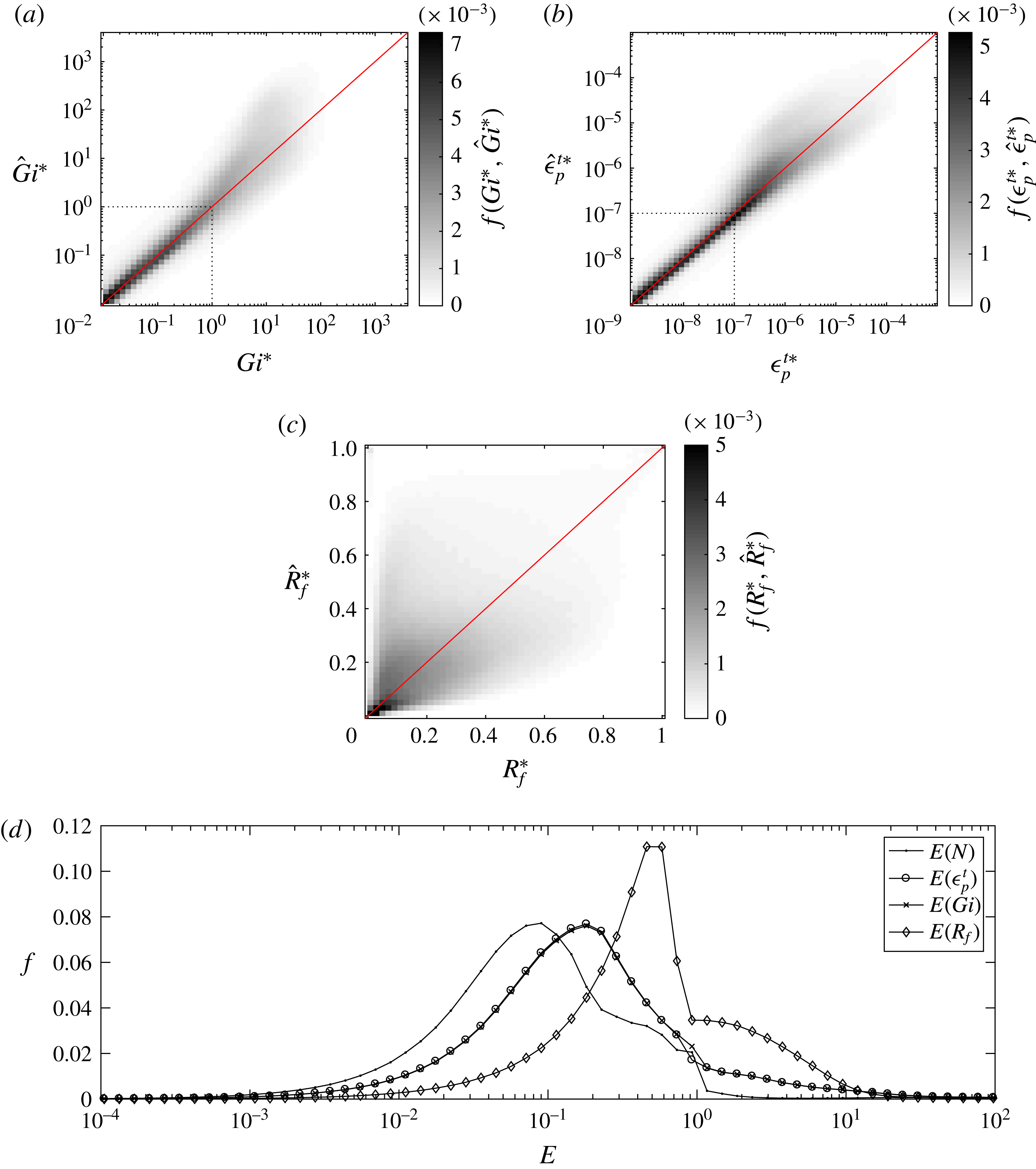
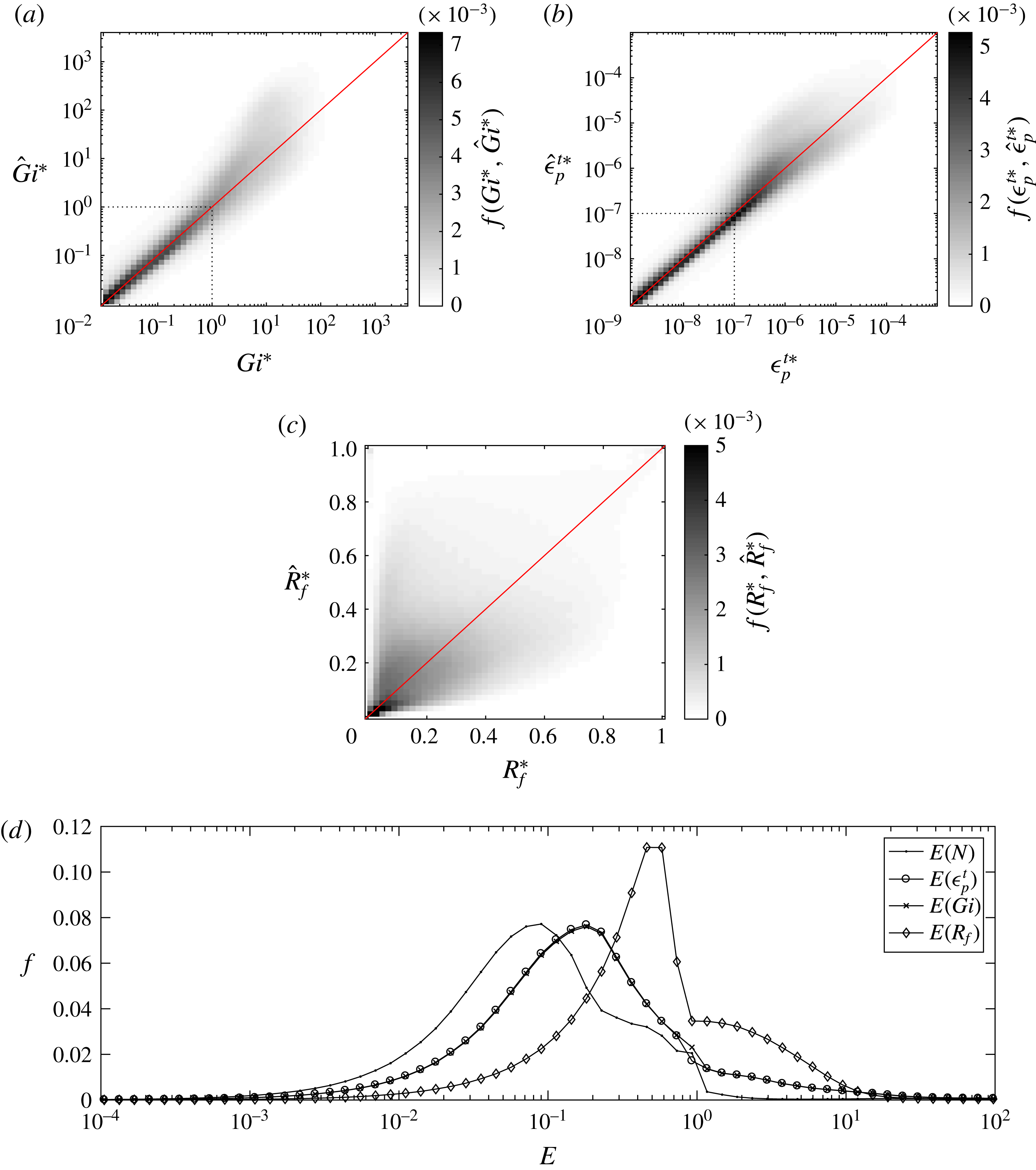
(a) Two-dimensional histogram of
 $f(Gi^{\ast },\hat{Gi}^{\ast })$
. (b) Two-dimensional histogram of
 $f(\unicode[STIX]{x1D716}_{p}^{t\ast },\hat{\unicode[STIX]{x1D716}}_{p}^{t\ast })$
. Here,
 $\unicode[STIX]{x1D716}_{p}^{t}$
is shown in units of
 $\text{m}^{2}~\text{s}^{-3}$
. (c) Two-dimensional histogram of
 $f(R_{f}^{\ast },\hat{R}_{f}^{\ast })$
. The
 $R_{f}$
calculations are limited to turbulent regions where
 $Gi>1$
. (d) Histogram of the error
 $E$
in calculations of
 $N$
,
 $\unicode[STIX]{x1D716}_{p}^{t}$
,
 $Gi$
and
 $R_{f}$
.
3.1 How turbulence quantities depend on the computation of
 $N$

Since
 $Gi$
is itself a function of the buoyancy frequency
 $N$
, it is first instructive to see how it varies with the method of computing
 $N$
. A direct comparison may be made using a two-dimensional histogram of
 $f(Gi^{\ast },\hat{Gi}^{\ast })$
(figure 2
a), which shows that
 $\hat{Gi}^{\ast }$
is generally greater than
 $Gi^{\ast }$
, especially for turbulent regions where
 $Gi>1$
. Because the calculation of
 $\unicode[STIX]{x1D716}_{k}^{t}$
is independent of the method used to compute
 $N$
, this indicates that
 $\hat{N}^{\ast }$
is generally less than
 $N^{\ast }$
. The two-dimensional histogram of
 $f(\unicode[STIX]{x1D716}_{p}^{t\ast },\hat{\unicode[STIX]{x1D716}}_{p}^{t\ast })$
(figure 2
b) provides further evidence that
 $\hat{N}^{\ast }$
underestimates
 $N^{\ast }$
. The term
 $\hat{\unicode[STIX]{x1D716}}_{p}^{t\ast }$
is generally larger than
 $\unicode[STIX]{x1D716}_{p}^{t\ast }$
, especially for larger mixing values (
 $\unicode[STIX]{x1D716}_{p}^{t}$
greater than roughly
 $1\times 10^{-7}~\text{m}^{2}~\text{s}^{-3}$
in figure 2
b). The observed differences in
 $\unicode[STIX]{x1D716}_{p}^{t}$
lead to differences in the flux Richardson number
 $R_{f}$
(figure 2
c):
 $\hat{R}_{f}^{\ast }$
is, overall, slightly larger than
 $R_{f}^{\ast }$
, as expected from the trend in
 $\unicode[STIX]{x1D716}_{p}^{t}$
. Most notably, for
 $R_{f}^{\ast }$
less than roughly 0.1, a region of increased
 $\hat{R}_{f}^{\ast }$
extends up to roughly 0.6, indicating large overestimates when lateral averaging and vertical sorting are used. It should be noted that
 $R_{f}$
quantities in figure 2 are limited to turbulent regions where
 $Gi>1$
.
If the
 $N$
value calculated from the three-dimensionally sorted density field is taken to be the true value, then the error caused by calculating
 $N$
using lateral averaging and vertical sorting can be defined as
 $$\begin{eqnarray}E(\unicode[STIX]{x1D719})=\frac{|\hat{\unicode[STIX]{x1D719}}^{\ast }-\unicode[STIX]{x1D719}^{\ast }|}{\unicode[STIX]{x1D719}^{\ast }},\end{eqnarray}$$
where
 $\unicode[STIX]{x1D719}$
is a turbulence quantity. The histogram in figure 2(d) shows that
 $E(N)$
is often
 $O(10^{-1})$
, and can be as large as
 $O(1)$
. It should be noted that, as discussed above,
 $\hat{N}^{\ast }$
is generally less than
 $N^{\ast }$
; thus, generally,
 $\hat{N}^{\ast }-N^{\ast }<0$
. However, the absolute value in (3.1) guarantees that
 $E>0$
, allowing it to be plotted on a log scale in figure 2(d). The error in
 $N$
translates to errors in
 $\unicode[STIX]{x1D716}_{p}^{t}$
,
 $Gi$
and
 $R_{f}$
as large as
 $O(10)$
. The terms
 $E(\unicode[STIX]{x1D716}_{p}^{t})$
and
 $E(Gi)$
are nearly identical, as they are both proportional to
 $1/N^{2}$
.
For the breaking wave scenarios considered here, lateral averaging and vertical sorting of density profiles unphysically smooth out variability in
 $N$
, leading to mixing estimates that are larger than the true mixing values. The variability in
 $N$
is better captured by full three-dimensional sorting, resulting in a more accurate measure of mixing. The additional (artificial) mixing that results from the use of
 $\hat{N}^{\ast }$
instead of
 $N^{\ast }$
can be quantified using an effective mixing coefficient
 $\unicode[STIX]{x1D705}_{eff}$
, defined with
 $$\begin{eqnarray}\hat{\unicode[STIX]{x1D716}}_{p}^{t\ast }=\unicode[STIX]{x1D705}\frac{\overline{|\unicode[STIX]{x1D735}b^{\prime }|^{2}}}{(\hat{N}^{\ast })^{2}}=\unicode[STIX]{x1D705}_{eff}\frac{\overline{|\unicode[STIX]{x1D735}b^{\prime }|^{2}}}{(N^{\ast })^{2}},\end{eqnarray}$$
which implies
 $$\begin{eqnarray}\unicode[STIX]{x1D705}_{eff}=\unicode[STIX]{x1D705}\left(\frac{N^{\ast }}{\hat{N}^{\ast }}\right)^{2}.\end{eqnarray}$$
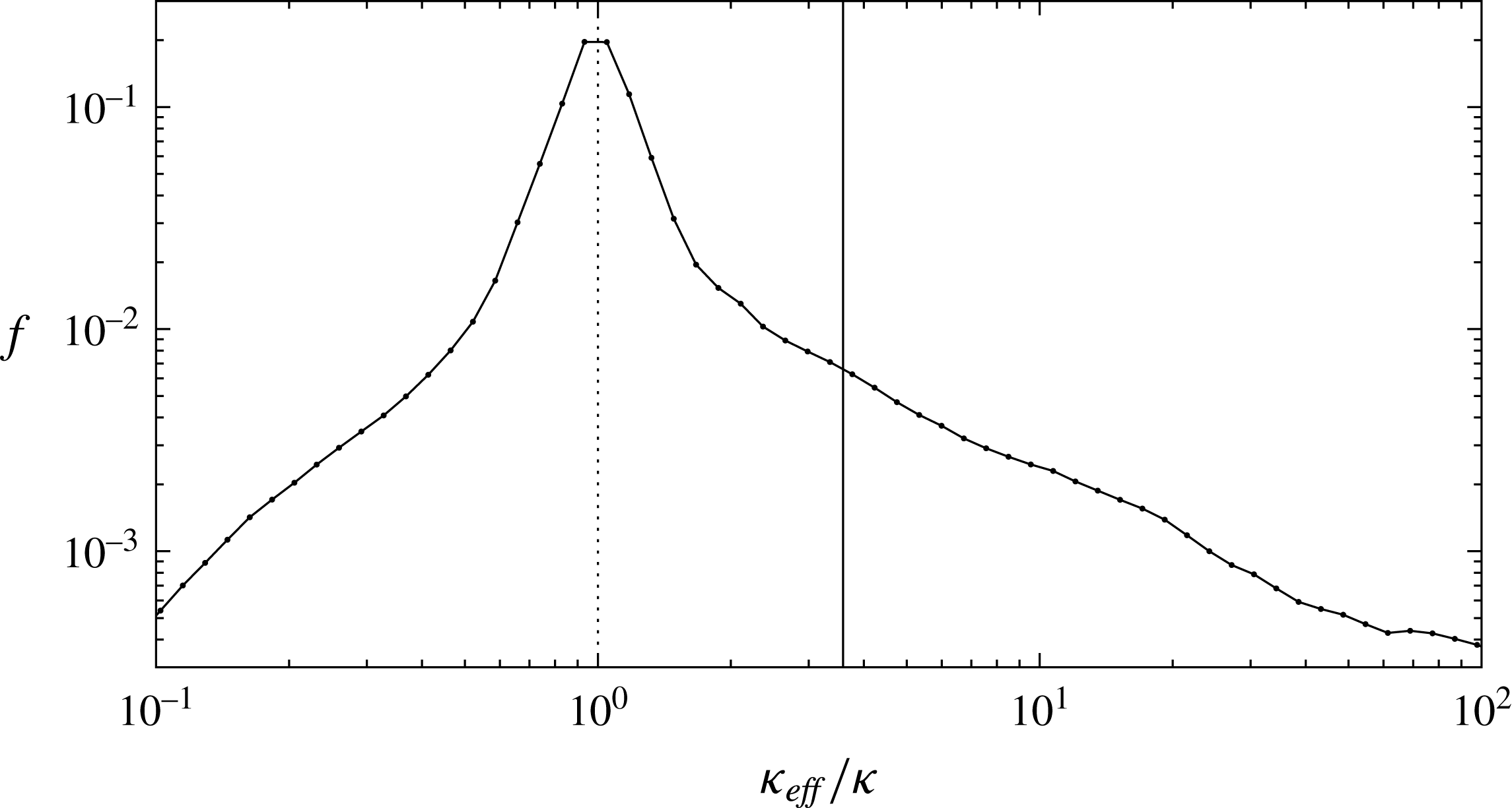
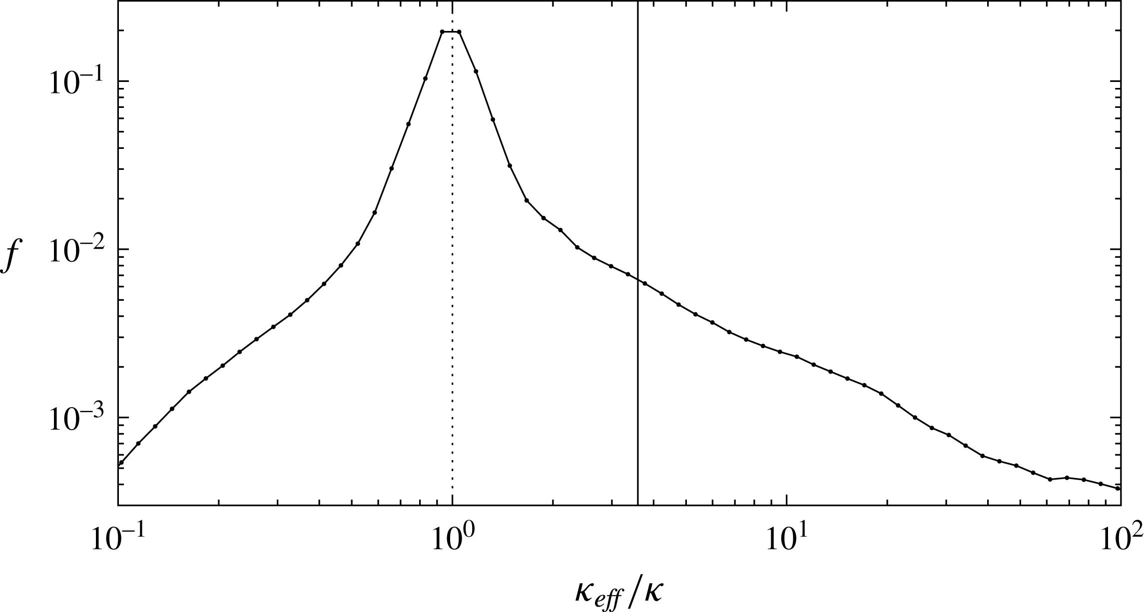
The effective mixing rate
 $\unicode[STIX]{x1D705}_{eff}$
is clearly skewed towards values larger than the true mixing rate
 $\unicode[STIX]{x1D705}$
, and is, on average, 3.6 times larger than
 $\unicode[STIX]{x1D705}$
(figure 3).
Histogram of the effective mixing rate
 $\unicode[STIX]{x1D705}_{eff}$
due to lateral averaging and vertical sorting. The vertical dotted line shows the true value of
 $\unicode[STIX]{x1D705}=1\times 10^{-6}~\text{m}^{2}~\text{s}^{-1}$
(Arthur et al. (Reference Arthur, Koseff and Fringer2017) use a Prandtl number
 $Pr=\unicode[STIX]{x1D708}/\unicode[STIX]{x1D705}=1$
). The vertical solid line shows the mean value of
 $\unicode[STIX]{x1D705}_{eff}/\unicode[STIX]{x1D705}=3.6$
.
3.2 The flux Richardson number
$R_{f}$
as a function of
$Gi$


The method of computing
 $N$
has a strong effect on the functional relationship between
 $R_{f}$
and
 $Gi$
, which is often used to parameterize mixing in the ocean. Here,
 $R_{f}$
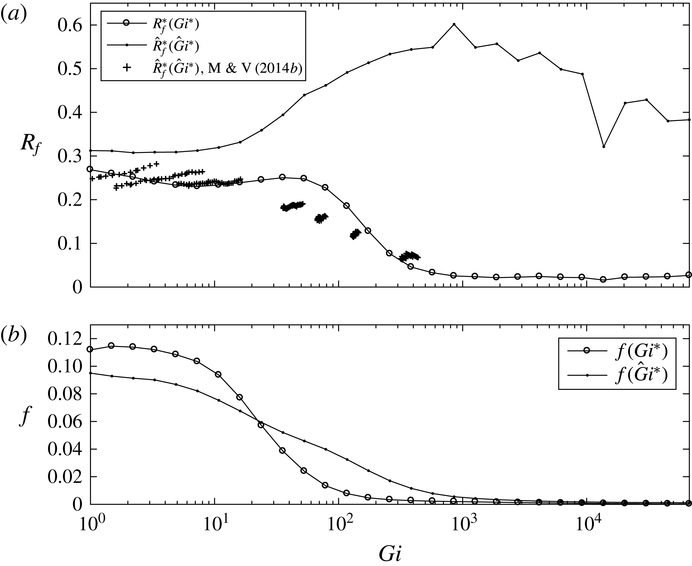
is calculated as a weighted mean in bins of
 $Gi$
(figure 4
a). As in the calculation of
 $f$
(described at the beginning of this section), area weighting is used to account for the non-uniform grid in the simulations of Arthur et al. (Reference Arthur, Koseff and Fringer2017). Thus, larger (smaller) grid cells, which take up a larger (smaller) portion of the computational domain, contribute more (less) to the mean value of
 $R_{f}$
. To show the spread of the data in terms of the Gibson number,
 $f$
is also calculated in each
 $Gi$
bin (figure 4
b). Due to computational restrictions on
 $Gi$
associated with the DNS, many of the data have relatively low (non-turbulent) values of
 $Gi<1$
. Since these values imply laminar flow, they are omitted in figure 4. It should be noted that calculations of
 $R_{f}$
for larger values of
 $Gi$
are based on a small subset of the data (figure 4
b), probably explaining the wiggles in the
 $\hat{R}_{f}^{\ast }$
curve.
(a) Comparison of mean
 $R_{f}^{\ast }$
as a function of
 $Gi^{\ast }$
with mean
 $\hat{R}_{f}^{\ast }$
as a function of
 $\hat{Gi}^{\ast }$
. The
 $\hat{R}_{f}^{\ast }$
calculation of Mater & Venayagamoorthy (Reference Mater and Venayagamoorthy2014b
) using the data of Shih et al. (Reference Shih, Koseff, Ivey and Ferziger2005) is included as well. (b) Histograms of
 $Gi^{\ast }$
and
 $\hat{Gi}^{\ast }$
.
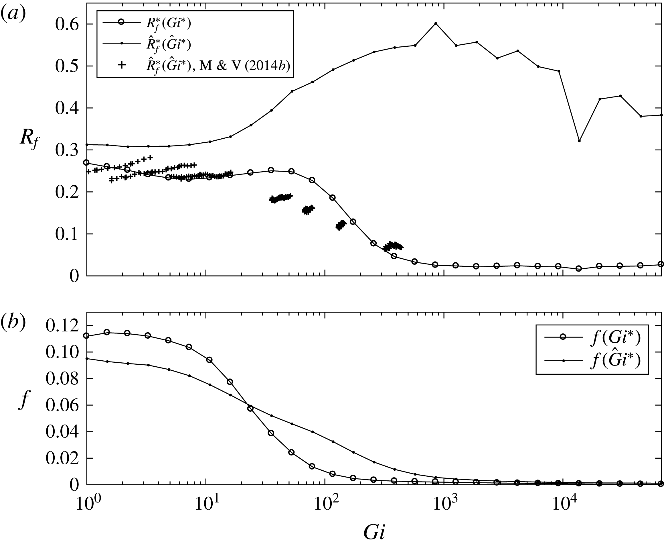
The term
 $\hat{R}_{f}^{\ast }$
, which reaches a peak of nearly 0.6 for
 $\hat{Gi}^{\ast }\approx 10^{3}$
, is generally larger than
 $R_{f}^{\ast }$
, which has maximum values between 0.2 and 0.3 for
 $Gi^{\ast }<10^{2}$
. For
 $Gi^{\ast }>10^{2}$
, a sharp drop in the mixing efficiency occurs and
 $R_{f}^{\ast }$
approaches 0. A similar result was found for
 $R_{f}$
by Shih et al. (Reference Shih, Koseff, Ivey and Ferziger2005), Walter et al. (Reference Walter, Squibb, Woodson, Koseff and Monismith2014) and others; see figure 12 in Walter et al. (Reference Walter, Squibb, Woodson, Koseff and Monismith2014). Because
 $\hat{Gi}^{\ast }$
is generally larger than
 $Gi^{\ast }$
, the decline of
 $\hat{R}_{f}^{\ast }$
for large values of
 $\hat{Gi}^{\ast }$
occurs at a larger value of
 $\hat{Gi}^{\ast }$
(approximately
 $\hat{Gi}^{\ast }=10^{3}$
).
The large discrepancies that arise in
 $R_{f}$
when lateral averaging and vertical sorting are used on unsteady inhomogeneous breaking wave data emphasize the potential effect of
 $N$
on mixing estimates in the ocean. If
 $Gi=10^{2}$
, local vertical sorting causes
 $R_{f}$
to be overestimated by roughly a factor of 2. This increases to a factor of roughly 10 when
 $Gi\geqslant 10^{3}$
. In contrast, the
 $\hat{R}_{f}^{\ast }(\hat{Gi}^{\ast })$
calculations of Mater & Venayagamoorthy (Reference Mater and Venayagamoorthy2014b
) using the stratified shear flow data of Shih et al. (Reference Shih, Koseff, Ivey and Ferziger2005) generally follow the present
 $R_{f}^{\ast }(Gi^{\ast })$
curve, but depart substantially from the present
 $\hat{R}_{f}^{\ast }(\hat{Gi}^{\ast })$
curve. This is probably due to the homogeneous nature of the turbulence studied by Shih et al. (Reference Shih, Koseff, Ivey and Ferziger2005), which could allow local vertical sorting to achieve a more accurate measure of the true background stratification. In the inhomogeneous flow studied here,
 $\hat{N}^{\ast }$
varies spatially, and may therefore be a less appropriate measure of
 $N$
.
4 Conclusion
Two different methods of computing the buoyancy frequency
 $N$
, one based on a three-dimensionally sorted density field and the other based on laterally averaged and vertically sorted density profiles, were used to calculate turbulent mixing quantities. For the breaking internal wave events considered here, the method of lateral averaging and vertical sorting (
 $\hat{N}^{\ast }$
) generally leads to a smaller value of the buoyancy frequency relative to full three-dimensional sorting (
 $N^{\ast }$
). Because
 $N$
represents the background stratification against which turbulence must work to stir the fluid, reduced values of
 $\hat{N}^{\ast }$
lead to overestimates of mixing relative to those calculated with
 $N^{\ast }$
. This, in turn, changes the functional relationship between the flux Richardson number
 $R_{f}$
and the turbulence activity number
 $Gi$
, which is commonly used to estimate mixing. These results have implications for how existing parameterizations of mixing in the ocean are used: the method of calculating
 $N$
not only affects
 $R_{f}$
, but also adds some uncertainty to its estimation using parameters, such as
 $Gi$
, that also depend on
 $N$
.
Acknowledgements
R.S.A. gratefully acknowledges the support of the Stanford Graduate Fellowship. R.S.A. and O.B.F. gratefully acknowledge the support of ONR grants N00014-08-1-0904 and N00014-16-1-2256 (scientific officers Dr C. Linwood Vincent, Dr T. Paluszkiewicz and Dr S. Harper). We gratefully acknowledge the US Army Research Laboratory DoD Supercomputing Resource Center for computer time on Pershing and Excalibur, and especially thank the diligent staff at the HPC Help Desk for their support. We also thank O. Murray of ONR for ensuring our access to these resources. Finally, we are grateful to two anonymous referees for their thoughtful reviews of the manuscript. A portion of this work was prepared by LLNL under Contract DE-AC52-07NA27344.