3.1. The development of a resilient control framework

Our aim is for the mechanical system to accurately follow the preset trajectory ${q}^{d}\left ( t\right )$ with a desired swift velocity $\dot {{q}^{d}}\left ( t\right )$ , assuming ${q}^{d}\left ( t\right )$ is defined on [ ${t}_{0}$ , $ \infty$ ] with continuous second-order differentiability, and both ${q}^{d}\left ( t\right )$ , its first derivative $\dot {{q}^{d}}\left ( t\right )$ , and second derivative $\ddot {{q}^{d}}\left ( t\right )$ are uniformly bounded:

(13) \begin{align} \begin{cases}\theta (t)=q(t)-{q}^{d}(t) \\[3pt]\dot {\theta }(t)=\dot {q}(t)-{\dot {q}}^{d}(t) \\[3pt]\ddot {\theta }(t)=\ddot {q}(t)-{\ddot {q}}^{d}(t) \end{cases} \end{align}

Let:

(14) \begin{equation} \widetilde {\theta }(t)={\left [ \theta (t)\dot {\theta }(t)\right ]}^{T} \end{equation}

Our objective is to ensure that the system’s state variable $\widetilde {\theta }(t)$ remains uniformly bounded under the control of the developed controller and ultimately achieves uniform ultimate boundedness. The dynamics of the joint module, as defined by Eq. (11), can be reconceptualized as follows:

(15) \begin{equation} E({\ddot {q}}^{d}(t)+\ddot {\theta }(t))+I({\dot {q}}^{d}(t)+\dot {\theta }(t))+F=\tau (t) \end{equation}

In fact, due to the uncertainty and variability of parameters, as well as the dynamic characteristics not fully described by the model, the system inherently contains uncertainty. Therefore, the dynamic model can be decomposed into a standard part and an uncertain part. The division of the functions $E\left ( \cdotp \right )$ , $I\left ( \cdotp \right )$ and $F\left ( \cdotp \right )$ can be understood in the following manner:

(16) \begin{equation} \begin{matrix}E(q,\sigma ,t)=\overline {E}(q,t)+\triangle E(q,\sigma ,t) \\[3pt] I(q,\dot {q},\sigma ,t)=\overline {I}(q,\dot {q},t)+\triangle I(q,\dot {q},\sigma ,t) \\[3pt] F(q,\dot {q},\sigma ,t)=\overline {F}(q,\dot {q},t)+\triangle F(q,\dot {q},\sigma ,t) \end{matrix} \end{equation}

In this context, $\overline {E}\left ( \cdotp \right )$ , $\overline {I}\left ( \cdotp \right )$ and $\overline {F}\left ( \cdotp \right )$ denote the baseline components, whereas the variations $\varDelta E$ , $\varDelta I$ and $\varDelta F$ signify the oscillating elements correlated with $\sigma$ .

Subsequently, the estimated range of uncertainty and external disturbances is denoted by the variable $ \rho$ . For a given positive value of S, the scalar function $ \rho$ is chosen in a manner that:

(17) \begin{equation} \left \| \phi (\theta ,\dot {\theta },\sigma ,t)\right \|\leqslant \rho (\theta ,\dot {\theta },\sigma ,t) \end{equation}

where:

(18) \begin{align} \phi (\theta ,\dot {\theta },\sigma ,t) &=-\triangle E(q,\sigma ,t)({\ddot {q}}^{d}-S\dot {\theta })-\triangle I(q,\dot {q},\sigma ,t)({\dot {q}}^{d} -S\theta)\nonumber \\ &\quad -\triangle F(\dot {q},\sigma ,t) \end{align}

The subsequent goal is to devise an efficient control strategy $\tau (t)$ that ensures the tracking error is confined within predefined limits. We can utilize an algorithm to guarantee the desired performance constraints [Reference Tang, Sun, Li and Song25]. With a positive value of $\epsilon$ (typically small) and positive tuning coefficients ${k}_{p}$ and ${k}_{v}$ , the control law for the nonlinear system can be derived as follows:

(19) \begin{equation} \tau (t)=\overline {E}({\ddot {q}}^{d}-S\dot {\theta })+\overline {I}({\dot {q}}^{d}-S\theta )+\overline {F}-{K}_{p}\theta -{K}_{v}\dot {\theta }+p(\theta ,\dot {\theta },t) \end{equation}

where

(20) \begin{align} p(\theta ,\dot {\theta },t)=\begin{cases} -\dfrac {\varphi (\theta ,\dot {\theta },t) }{\epsilon }\rho (\theta ,\dot {\theta },t),& if\left \|\varphi (\theta ,\dot {\theta },t) \right \|\leqslant \epsilon \\[7pt] -\dfrac {\varphi (\theta ,\dot {\theta },t) }{\left \|\varphi (\theta ,\dot {\theta },t) \right \|}\rho (\theta ,\dot {\theta },t),& if\left \|\varphi (\theta ,\dot {\theta },t) \right \|\gt \epsilon \end{cases} \end{align}

(21) \begin{equation} \varphi (\theta ,\dot {\theta },t)=(\dot {\theta }+S\theta )\rho (\theta ,\dot {\theta },t) \end{equation}

(22) \begin{equation} {K}_{p}=diag{\left [ {K}_{pi}\right ]}_{n*n} \end{equation}

(23) \begin{equation} {K}_{v}=diag{\left [ {K}_{vi}\right ]}_{n*n} \end{equation}

Through in-depth analysis, our proposed model-based PD robust control framework demonstrates a design that relies on accurate system modeling and fully leverages the advantages of the PID control mechanism. The proportional adjustment component of the controller is designed to neutralize external disturbances and system uncertainties, with its piecewise design effectively preventing an excessive increase in robustness as the control signal decreases. This theoretical framework suggests that the FHPD controller surpasses standard PID and MPD controllers in terms of dynamic response. Figure 2 comprehensively displays the controller configuration, explaining how model-driven components and the PD feedback loop work together to reduce the discrepancy between the target and actual positions. In addition, the proportional component effectively alleviates uncertainties from the mechanical system and external disturbances, significantly enhancing the system’s dynamic performance.

Figure 2.

Proposed FHPD robust control architecture diagram.

After structural analysis of the proposed controller, its advantages can be rephrased as follows:

1. 1. Our algorithm, an extension of the traditional PD control, simplifies the complexity of parameter adjustment for engineering applications, enhancing its practicality.

2. 2. The algorithm not only streamlines the parameter tuning process but also demonstrates robustness against uncertainties in parameters and external disturbances.

3. 3. With a design that emphasizes simplicity and ease of implementation, the controller requires minimal hardware resources, making it suitable for a variety of mechanical systems with common embedded chips.

The design process of the PD robust controller for the joint module system can be re-articulated as:

Step one: Establish the dynamic equation of the joint module system using the Lagrangian approach.

Step two: Determine the upper bounds of external disturbances and uncertainties within the system, and calculate the scalar function q through Eq. (17).

Step three: Construct a piecewise function for q based on Eqs. (20) and (21).

Step four: Develop a model-based PD robust control method according to Eq. (19).

Considering the comprehensive analysis of the controller and its design process, it is notable that our proposed controller, with its low hardware requirements and ease of adjusting control parameters, is not only applicable to motor-driven systems but can also be rapidly adapted and integrated into various types of mechanical systems to achieve the desired motion control effects.

3.2. Stability analysis

Theorem. The controller (19) maintains the joint module’s error term $\widetilde {\theta }\left ( t\right )$ within a predefined boundary and ensures its convergence to a steady state within this boundary. The selection of an appropriate value for $\epsilon$ allows for the minimization of the error’s steady-state boundary, aligning with the precision objectives.

1. 1. Uniform boundedness: For any $\gamma \gt 0$ ,there exists a finite $d\left ( \gamma \right )$ such that the norm of $q\left ( t\right )$ does not exceed $d\left ( \gamma \right )$ for all times $t$ greater than or equal to ${t}_{0}$ , provided that the initial condition $\left \| q\left ( {t}_{0}\right )\right \|$ is less than or equal to $\gamma$ , $\left \| q\left ( t\right )\leqslant d\left ( \gamma \right )\right \|$ for all $t\geqslant {t}_{0}$ , as shown in the left part of Figure 3.

2. 2. Uniform ultimate boundedness: Given $\gamma \gt 0$ , if the initial condition $\left \| q\left ( {t}_{0}\right )\right \|$ is within the bound $\gamma$ , there exists a positive d such that the norm of $q\left ( t\right )$ will be at least $d$ for all future times $t$ beyond ${t}_{0}+ T\left ( \bar {d},\gamma \right )$ , where $T\left ( \bar {d},\gamma \right )$ is a finite time that depends on $\bar {d}$ and $\gamma$ , $\left \| q\left ( t\right ) \right \|\geqslant d$ for all $t\geqslant {t}_{0}+ T\left ( \bar {d},\gamma \right )$ with $\bar {d}\gt d$ and $T\left ( \bar {d},\gamma \right )\lt \infty$ , as shown in the right part of Figure 3.

Figure 3.

System performance.

Proof. By employing the Lyapunov minimax approach, the stability assessment of the proposed controller is executed. Functions $d\left ( r\right )$ and $\bar {d}$ are established to ensure the system’s uniform boundedness and ultimate boundedness, enabling the closed-loop system to achieve the target error threshold in a finite timeframe. In the process of substantiating the controller’s stability, the subsequent discussion elaborates on the criteria for selecting an appropriate Lyapunov function candidate:

(24) \begin{equation} V(\widetilde {\theta },t)=\frac {1}{2}{(\dot {\theta }+S\theta )}^{T}E(\dot {\theta }+S\theta )+\frac {1}{2}{\theta }^{T}({K}_{p}+S{K}_{v})\theta \end{equation}

The Hamiltonian function $E\left ( q\right )$ of the mechanical system is confirmed to be uniformly positive definite, indicating the presence of a constant $\delta$ that satisfies this condition:

(25) \begin{equation} E(q)\geqslant \delta I\, \, \, \, \forall q\in {R}^{n} \end{equation}

To verify that V is a Lyapunov function, it is necessary to demonstrate that V is both positive definite and monotonically decreasing [Reference Slotine and Li26]. Given that Eq. (25) ensures the boundedness of E, the analysis can proceed as follows:

(26) \begin{align} V(\widetilde {\theta },t) &\geqslant {\frac {1}{2}\delta \left \| \dot {\theta }+S\theta \right \|}^{2}+\frac {1}{2}{\theta }^{T}({K}_{p}+S{K}_{v})\nonumber\\[4pt]&=\frac {1}{2}\delta ({\theta }^{2}+2S\dot {\theta }\theta +{S}^{2}{\theta }^{2})+\frac {1}{2}\delta ({K}_{p}+S{K}_{v}){\theta }^{2} \nonumber \\[4pt]&=\frac {1}{2}[\theta \dot {\theta }]\psi [\theta \dot {\theta }] \end{align}

where

(27) \begin{equation} \psi =\begin{bmatrix} \delta +{K}_{p}+S{K}_{v} & \delta S\\ \delta S & \delta \end{bmatrix} \end{equation}

Demonstrating that $\psi$ is positive is straightforward, which confirms that V is positive definite.

(28) \begin{equation} V\geqslant \frac {1}{2}{\lambda }_{min}(\psi )({\theta }^{2}+{\dot {\theta }}^{2})\geqslant \frac {1}{2}\underline {\lambda }{\left \| \theta \right \|}^{2} \end{equation}

where $\underline {\lambda }=min \,{\lambda }_{min}(\psi ),\, \, \, \, \underline {\lambda }\geqslant 0$ . This indicates that V is positive definite.

The change rate of V along the trajectory can be outlined as follows:

(29) \begin{align} \dot {V}&={(\dot {\theta }+S\theta )}^{T}(\tau -E{\ddot {q}}^{d}-I(\dot {\theta }+{\dot {q}^{d}})-F+ES\dot {\theta })\nonumber\\[3pt] &\qquad+\frac {1}{2}{(\dot {\theta }+S\theta )}^{T}\dot {\theta }(\dot {\theta }+S\theta )+{\theta }^{T}({K}_{p}+S{K}_{v})\dot {\theta }\nonumber\\[3pt] &={(\dot {\theta }+S\theta )}^{T}(\tau -E({\ddot {q}}^{d}-S\dot {\theta })-I({\dot {q}}^{d}-S\theta )-F) \nonumber\\[3pt] &\qquad-{(\dot {\theta }+S\theta )}^{T}I(\dot {\theta }+S\theta )+\frac {1}{2}{(\dot {\theta }+S\theta )}^{T}\dot {E}(\dot {\theta }+S\theta )\nonumber\\[3pt] &\qquad+{\theta }^{T}({K}_{p}+S{K}_{V})\dot {\theta } \end{align}

By Eq. (19) and using Eq. (29),

(30) \begin{align} \dot {V}&={(\dot {\theta }+S\theta )}^{T}[(\overline {E}-E)({\ddot {q}}^{d}-S\dot {\theta })+(\overline {I}-I)({\dot {q}}^{d}-S\theta )\nonumber\\[3pt] &\qquad+\overline {F}-F+p]-{(\dot {\theta }+S\theta )}^{T}({K}_{p}e+{K}_{v}\dot {\theta })+{\theta }^{T}({K}_{p}+S{K}_{v})\dot {\theta }\nonumber\\[3pt] &={(\dot {\theta }+S\theta )}^{T}\phi +{(\dot {\theta }+S\theta )}^{T}p-{\dot {\theta }}^{T}{K}_{v}\dot {\theta }-{\theta }^{T}S{K}_{p}\theta \end{align}

if $\left \| \varphi \right \|\gt \epsilon$ , then

(31) \begin{equation} {(\dot {\theta }+S\theta )}^{T}p=-\frac {{(\dot {\theta }+S\theta )}^{T}(\dot {\theta }+S\theta )\rho }{\left \| \varphi \right \|}\rho =-\left \| \varphi \right \| \end{equation}

if $\left \| \varphi \right \|\leqslant \epsilon$ , then

(32) \begin{equation} {(\dot {\theta }+S\theta )}^{T}p=-\frac {{(\dot {\theta }+S\theta )}^{T}(\dot {\theta }+S\theta )\rho }{\left \| \epsilon \right \|}\rho =-\frac {{\left \| \varphi \right \|}^{2}}{\epsilon } \end{equation}

Therefore, by Eqs. (21), (31) and (32), we get,

(33) \begin{equation} {(\dot {\theta }+S\theta )}^{T}\phi + {(\dot {\theta }+S\theta )}^{T}p \leqslant {(\dot {\theta }+S\theta )}^{T}p+\left \| \varphi \right \| \end{equation}

If $\left \| \varphi \right \|\gt \epsilon$ (31), we are able to derive

(34) \begin{equation} {(\dot {\theta }+S\theta )}^{T}p+{(\dot {\theta }+S\theta )}^{T}\phi \leqslant 0 \end{equation}

If $\left \| \varphi \right \|\leqslant \epsilon$ (32), we are able to derive

(35) \begin{equation} \frac {\epsilon }{4}\geqslant \left \| \varphi \right \|-\frac {{\left \| \varphi \right \|}^{2}}{\epsilon }\geqslant {(\dot {\theta }+S\theta )}^{T}\phi + {(\dot {\theta }+S\theta )}^{T}p \end{equation}

Consequently, when $\epsilon \gt 0$ , inequality (35) is valid for all $\epsilon$ . Substituting (35) into Eq. (30) yields the following result:

(36) \begin{equation} \frac {\epsilon }{4}-{\underline {\lambda }}_{1}{\left \| \widetilde {\theta }\right \|}^{2}\geqslant \dot {V} \end{equation}

where

(37) \begin{equation} {\underline {\lambda }}_{1}=min \left \{ {K}_{v},S{K}_{p}\right \} \end{equation}

Actually, for all norms $\left \|\widetilde {\theta } \right \|$ that meet the specified criteria, the value of V will be negative:

(38) \begin{equation} \frac {\epsilon }{4}-{\underline {\lambda }}_{1}{\left \| \widetilde {\theta }\right \|}^{2}\lt 0 \end{equation}

The purpose of these properties is to ensure the consistency of the boundary. In other words, for any given $\gamma \gt 0$ and $\left \| \tilde {\theta }\left ( {t}_{0}\right )\right \|\leqslant \gamma$ (where ${t}_{0}$ represents the initial time), the following inequality always holds:

(39) \begin{align} d(r)=\begin{cases} R{\left [ \dfrac {2({\overline {\lambda }}_{0}+{\overline {\lambda }}_{1}R+{\overline {\lambda }}_{2}{R}^{2})}{\underline {\lambda }}\right ]}^{\tfrac {1}{2}},& if\; \; r\leqslant R \\[10pt] r{\left [ \dfrac {2({\overline {\lambda }}_{0}+{\overline {\lambda }}_{1}r+{\overline {\lambda }}_{2}{r}^{2})}{\underline {\lambda }}\right ]}^{\tfrac {1}{2}},& if\; \; r\gt R \end{cases} \end{align}

(40) \begin{equation} R={\left [ \frac {\epsilon }{4{\underline {\lambda }}_{1}}\right ]}^{\frac {1}{2}} \end{equation}

Uniform ultimate boundedness can be guaranteed, meaning that $\left \| \tilde {e\left ( t\right )}\right \|$ will not exceed $d\left ( r\right )$ for all $t \geqslant {t}_{0}$ . Essentially, this holds true for any given $\bar {d}$ :

(41) \begin{equation} \overline {d}\gt R{\left [ \frac {2({\overline {\lambda }}_{0}+{\overline {\lambda }}_{1}R+{\overline {\lambda }}_{2}{R}^{2})}{\underline {\lambda }}\right ]}^{\frac {1}{2}} \end{equation}

By employing the following methods, the system’s performance can be guaranteed [Reference Corless and Leitmann27]:

(42) \begin{equation} T(\overline {d},r)=\begin{cases} 0,& if\; \; r\leqslant \overline {R} \\ \dfrac {{\overline {\lambda }}_{0}{r}^{2}+{\overline {\lambda }}_{1}{r}^{3}+{\overline {\lambda }}_{2}{r}^{4}-\frac {1}{2}\underline {\lambda }{\overline {R}}^{2}}{\underline {\lambda }{\overline {R}}^{2}-\frac {\epsilon }{4}},& if\; \; r\geqslant \overline {R} \end{cases} \end{equation}

(43) \begin{equation} \overline {R}={r}_{2}^{-1}\left ( \frac {1}{2}\underline {\lambda }{\overline {d}}^{2}\right ) \end{equation}

(44) \begin{equation} {r}_{2}(\zeta )={\overline {\lambda }}_{0}{\zeta }^{2}+{\overline {\lambda }}_{1}{\zeta }^{3}+{\overline {\lambda }}_{2}{\zeta }^{4} \end{equation}

By choosing $a$ suitably, the size of the terminal bounded region [Reference Bechlioulis and Rovithakis28] can be made arbitrarily small for all $t \geqslant {t}_{0} + T\left (\bar {d}, r\right )$ , provided that $\left \| \tilde {\theta }\left ( t\right )\right \|\leqslant \bar {q}$ .

3.3. Simulation

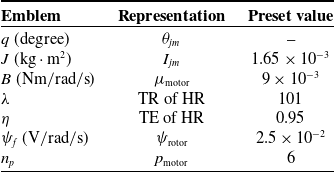
This paper employs numerical simulation to assess the efficacy of the robust elastic control strategy. Key parameters of the disc motor are detailed in Table I, which are then used to calculate Eq. (11), yielding the matrix in Eq. (15) that forms the basis for the simulation analysis.

In assessing the relative performance of PID, MPD, ADRC and FHPD in position tracking tasks, we utilized both step and sinusoidal inputs for our experiments, facilitating a comprehensive evaluation of the data obtained.

Table I.

Constituents and variables of the joint module mechanism.

Table II.

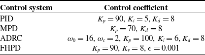
Variables within control strategies.

After thorough testing of the control parameters for three algorithms to ensure a fair comparison and to find a balance between system stability and response speed, we determined the optimal parameter settings as shown in Table II. In the simulation of the FHPD control strategy, the uncertainty introduced by the cosine function had a relatively minor impact on the disc motor.

Figure 4.

Disc motor’s sine wave tracking simulation results.

Figure 5.

Sinusoidal signal tracking.

However, when the motor was subjected to sinusoidal disturbances, the impact was significantly greater compared to square wave disturbances. Based on this finding, we decided to adopt the formula $\hat {F}= 0.5+0.01* \sin \left ( 5t\right )$ to represent the uncertainty factor of the motor. The initial error $e\left (\circ \right )$ was set to zero at the start of the experiment, and a fixed sampling interval of 0.001 s was chosen.

1. 1. Step Response Test: The amplitude of the step signal, denoted as ${q}^{d}$ , is set to $51.0556^{\circ }$ . The corresponding results are displayed in Figure 4. It was noted that the FHPD controller achieved the target trajectory more swiftly and without any overshoot, outperforming both the PID and MPD controllers.

2. 2. Sinusoidal Signal Tracking: The sinusoidal signal is considered as the reference path for tracking with amplitude $80.6686^{\circ }$ .

Figures 5 presents the simulation results for a sinusoidal signal tracking scenario using a Stribeck friction model. The system’s initial response to the sinusoidal signal was similar to that of a step input scenario. Upon reaching a steady state, the FHPD controller demonstrated a reduction in steady-state error and a shorter time to recovery compared to the PID and MPD controllers, exhibiting a swifter return to stability. The findings from these simulations indicate that the discussed controller is effective in enhancing the system’s dynamic response capabilities.

Figure 6.

The experimental platform known as CSPACE.

3.4. Experiment

A series of experiments focusing on the disc motor have been conducted to thoroughly verify the applicability of the control algorithm. As depicted in Figure 6, the experimental setup includes a computer, cSPACE supervisory software, a cSPACE control unit, and a disc motor embedded in a hip-assisting exoskeleton robot, among other equipment. An encoder with a 2500-line incremental count capability is utilized to collect positional data of the motor, with the simulation tests employing identical parameter settings.

The experimental procedure consists of three main stages: Firstly, the positional signals of the motor are acquired by the incremental encoder and fed back to the controller; Secondly, the digital signal processor within the cSPACE system, in accordance with our proposed control strategy, receives and processes the incoming data; Lastly, the motor is driven by augmenting the control signal, thereby achieving precise motion control of the disc motor.

1. 1. Transient performance in the simulation experiments in Figure 7 illustrates the effect of the FHPD control strategy on the disc motor’s response to a step signal. The FHPD controller not only achieves rapid stabilization but also maintains high control precision, with errors being smaller and exhibiting superior convergence speed compared to other controllers.

2. 2. Steady-state Performance, Figure 8, compares the performance of the three control strategies in the sinusoidal signal tracking experiment. Additionally, as can be seen from Figure 8, the FHPD control strategy outperforms PID and MPD in terms of accuracy, which is consistent with the simulation analysis. The highest tracking errors typically occur when the disc motor’s speed is near zero, mainly due to the imprecision of the position sensor and static friction. The experimental results indicate that there is almost no difference in control current among the three approaches.

Figure 9 presents a comparative analysis of current waveforms for the FHPD, MPD, and PID controllers during experimental operation. The results indicate that the FHPD controller achieves significantly reduced current oscillations compared to the other methods, demonstrating enhanced stability and energy efficiency. Notably, the FHPD exhibits lower peak currents and reduced fluctuations, which directly translate to decreased energy consumption. This improved performance is attributed to the FHPD’s optimized control strategy, which minimizes unnecessary power usage while maintaining precise tracking. The figure clearly illustrates the practical benefits of the FHPD controller in real-world applications.

Figure 7.

The experiment results of step response analysis.

Figure 8.

Sinusoidal response analysis.

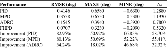
Table III presents a summary and comparison of the experimental findings. This comparison includes key performance indicators such as the root mean square error (RMSE), maximum error (MAXE), minimum error (MINE), and the range of error ( $\Delta _{\theta }$ ).

(45) \begin{equation} M A X E=\max \left (\left |\theta _{i}\right |\right ) \end{equation}

(46) \begin{equation} M I N E=\min \left (\left |\theta _{i}\right |\right ) \end{equation}

(47) \begin{equation} R M S E=\sqrt {\frac {1}{n} \sum _{i=1}^{n} \theta _{i}^{2}} \end{equation}

(48) \begin{equation} \Delta _{\theta }=\theta _{M A X E }-\theta _{M I N E } \end{equation}

Table III.

Comparison of control response performance of different control methods.

Figure 9.

Current waveform comparison.

The variable $ n$ indicates the total number of samples, while $ \theta _i$ signifies the tracking error for each individual sample $ i$ . The analysis indicates that the FHPD controller exhibits significant improvements in tracking accuracy and robustness compared to the PID, MPD, and ADRC methods. The FHPD controller demonstrates a substantial reduction in both RMSE and MAXE, along with a narrower error range, which underscores its enhanced performance and stability. These improvements are particularly important for maintaining consistent performance across various experimental conditions, highlighting the FHPD controller’s effectiveness in handling uncertainties such as tracking errors.

To comprehensively evaluate the performance of the FHPD controller against traditional PID and MPD controllers, we have incorporated several illustrative figures. The left figure in Figure 10 presents a bar chart comparing the tracking error range width from the sinusoidal tracking experiment, clearly highlighting the disparities in error ranges among the three methods. The results demonstrate that the proposed FHPD controller achieves a tracking error of $0.532^{\circ }$ , representing a 58.70% reduction compared to the traditional PID controller ( $1.288^{\circ }$ ) and a 55.41% reduction compared to the traditional MPD controller ( $1.193^{\circ }$ ). Additionally, the FHPD controller outperforms ADRC ( $0.786^{\circ }$ ) by reducing the tracking error by 32.32%. These findings highlight the superior performance of the FHPD controller in tracking accuracy. The right figure in Figure 11 offers a radar chart depicting the improvement percentages of the FHPD method relative to the others, visually emphasizing its significant performance enhancement. The left figure in Figure 11 displays a bar chart contrasting the stability difference width between simulation and experimental results in the step response test, demonstrating the FHPD controller’s consistent performance across both scenarios. The right figure in Figure 10 provides a bar chart of the difference percentages between simulation and experimental results for the three methods, further substantiating the reliability of the FHPD controller. Together, these visual aids effectively elucidate the performance variations among different control methods and underscore the superiority of the proposed FHPD controller.