1 Introduction
The boundary layer (BL) is an important concept in science and engineering, which was introduced more than 100 years ago by Prandtl (Reference Prandtl and Krazer1904) and has had a profound impact in fluid physics, aerodynamics and applied mathematics (Anderson Reference Anderson2005). It also has a close connection to many practical engineering problems ranging from skin friction drag to mass and heat transfer near a solid surface. Our current theoretical understanding of BL dynamics is limited to two flow regimes. At the low velocity limit, where the fluid flow is laminar, one can solve the BL equations and obtain the well-known Prandtl–Blasius–Pohlhausen (PBP) solution (Landau & Lifshitz Reference Landau and Lifshitz1987) as one example of a class of similarity solutions (Schlichting & Gersten Reference Schlichting and Gersten2000). At the high velocity limit, where the nonlinear effect becomes dominant, the BL is turbulent and extends into the bulk region of the flow. In this case, a logarithmic velocity (or temperature) profile was predicted (Kraichnan Reference Kraichnan1962; Spiegel Reference Spiegel1971; Shraiman & Siggia Reference Shraiman and Siggia1990; Grossmann & Lohse Reference Grossmann and Lohse2011). In fact, there is a large class of BL flows remaining between the two limiting cases.
The thermal BL in turbulent Rayleigh–Bénard convection (RBC) with the Rayleigh number (dimensionless buoyancy)
 $Ra<10^{14}$
is an example in which the BL is not fully turbulent but there are significant fluctuations resulting from intermittent eruption of thermal plumes from the BL. In the laboratory, RBC is realized in a confined fluid layer of height
 $H$
, which is heated from below and cooled from the top with a vertical temperature gradient parallel to gravity. When the temperature difference
 $\unicode[STIX]{x0394}T$
across the fluid layer is large enough, the bulk fluid becomes turbulent and heat is transported predominantly by convection. As a wall-bounded flow, RBC has temperature and velocity BLs adjacent to the upper and lower conducting plates. The structure and dynamics of the temperature BL are of great importance, as they determine the global heat transport of the system (Kadanoff Reference Kadanoff2001; Ahlers, Grossmann & Lohse Reference Ahlers, Grossmann and Lohse2009).
Recently, Shishkina et al. (Reference Shishkina, Horn, Wagner and Ching2015) considered the effect of BL fluctuations in RBC and included the velocity–temperature correlation function,
 $\langle v^{\prime }T^{\prime }\rangle$
, in the two-dimensional (2-D) BL equation for the normalized mean temperature profile
 $\unicode[STIX]{x1D703}(z)$
(with
 $z$
being the distance away from the solid surface), where
 $T^{\prime }$
and
 $v^{\prime }$
are, respectively, the local temperature and vertical velocity fluctuations, and
 $\langle \cdots \rangle$
denotes an average over time
 $t$
. Under the assumptions that the thermal BL is nested inside the velocity BL, that
 $$\begin{eqnarray}\langle v^{\prime }T^{\prime }\rangle =-(a\unicode[STIX]{x1D709}^{3}\unicode[STIX]{x1D705})\unicode[STIX]{x2202}_{z}\langle T\rangle ,\end{eqnarray}$$
and that a turbulent thermal diffusivity is given by
 $$\begin{eqnarray}\unicode[STIX]{x1D705}_{t}=a\unicode[STIX]{x1D709}^{3}\unicode[STIX]{x1D705},\end{eqnarray}$$
with
 $\unicode[STIX]{x1D705}$
being the molecular thermal diffusivity of the convecting fluid and
 $a$
a numerical constant, Shishkina et al. (Reference Shishkina, Horn, Wagner and Ching2015) obtained an analytical expression for the mean temperature profile. It is given by
 $$\begin{eqnarray}\unicode[STIX]{x1D703}(\unicode[STIX]{x1D709};c)\equiv \frac{T_{b}-\langle T(\unicode[STIX]{x1D709})\rangle }{\unicode[STIX]{x1D6E5}_{b}}=\int _{0}^{\unicode[STIX]{x1D709}}(1+a\unicode[STIX]{x1D702}^{3})^{-c}\,\text{d}\unicode[STIX]{x1D702}.\end{eqnarray}$$
Here,
 $\unicode[STIX]{x1D6E5}_{b}\equiv T_{b}-T_{0}$
is the temperature difference across the BL with
 $T_{b}$
and
 $T_{0}$
being, respectively, the temperature of the bottom plate and at the cell centre, and
 $\unicode[STIX]{x1D709}\equiv z/\unicode[STIX]{x1D6FF}$
is the vertical distance from the conducting plate normalized by the thermal BL thickness
 $\unicode[STIX]{x1D6FF}$
. Hereafter,
 $\unicode[STIX]{x1D709}$
is used directly in all equations to simplify the notation and
 $z/\unicode[STIX]{x1D6FF}$
is used in the presentation of the experimental and numerical data to indicate that they are actually measured as a function of
 $z$
. In the above, the constant
 $a$
is a dimensionless measure of turbulent diffusivity and is related to the constant
 $c$
(
 ${\geqslant}1$
) by the requirement
 $\unicode[STIX]{x1D703}(\infty )=1$
. This condition gives
 $$\begin{eqnarray}a=\left(\frac{\unicode[STIX]{x1D6E4}(1/3)\unicode[STIX]{x1D6E4}(c-1/3)}{3\unicode[STIX]{x1D6E4}(c)}\right)^{3},\end{eqnarray}$$
where
 $\unicode[STIX]{x1D6E4}(x)$
is the gamma function. Numerically,
 $a$
is a monotonic decreasing function of
 $c$
, with
 $a\simeq 1.77$
at
 $c=1$
and
 $a\simeq 0.21$
at
 $c=4$
. The value of
 $a$
for larger values of
 $c$
slowly decays to zero as
 $c\rightarrow \infty$
. In this limit,
 $\unicode[STIX]{x1D703}(\unicode[STIX]{x1D709};\infty )$
approaches the PBP form for laminar BLs without BL fluctuations.
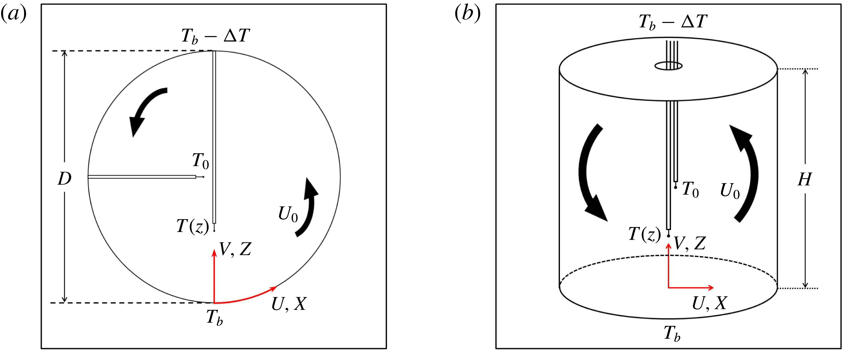
Sketch of the experimental set-up for the measurement of the local temperature profiles near the lower conducting plate in the vertical thin disk (a) and in the
 $\unicode[STIX]{x1D6E4}=1$
upright cylinder (b). The black arrows indicate the direction of the large-scale circulation with speed
 $U_{0}$
. The red arrows indicate the velocity components and spatial coordinates used in the experiment.

Equation (1.3) was tested in a recent convection experiment (Wang, He & Tong Reference Wang, He and Tong2016), which was conducted in a vertical thin disk with its circular cross-section aligned parallel to gravity (see figure 1(a) for more details). This is a specially designed quasi-2-D cell for RBC without any corner in order to prevent secondary flows. The large-scale flow in the circular cross-section of the cell has a fly-wheel-like structure with a mean rotating speed
 $U_{0}$
along a fixed orientation. Because the flow is confined in a thin circular disk, no other flow modes can be excited in this quasi-2-D system. Compared with the large-scale flow in a conventional upright cylinder, this quasi-2-D flow has a better geometry satisfying the assumption of the BL theory for a 2-D flow over an infinite horizontal plane. These simplifications allow us to have a stringent test of the theory. It was found that the measured
 $\unicode[STIX]{x1D703}(z)$
has a scaling form
 $\unicode[STIX]{x1D703}(z/\unicode[STIX]{x1D6FF})$
in the
 $Ra$
range studied, which is well described by (1.3) and the value of the fitting parameter
 $c$
was found to change sensitively with the Prandtl number
 $Pr=\unicode[STIX]{x1D708}/\unicode[STIX]{x1D705}$
, where
 $\unicode[STIX]{x1D708}$
is the kinematic viscosity of the convecting fluid. The experiment was performed with
 $Ra$
varied in the range
 $1.5\times 10^{9}\lesssim Ra\lesssim 1.3\times 10^{10}$
and
 $Pr$
was fixed. Two working fluids were used; one was distilled water (with
 $Pr=4.4$
) and the other was a 20 wt.% aqueous solution of glycerine (
 $Pr=7.6$
).
In addition to the mean temperature profile
 $\unicode[STIX]{x1D703}(z)$
, Wang et al. (Reference Wang, He and Tong2016) also measured the temperature variance profile
 $\unicode[STIX]{x1D702}(z)\equiv \langle [T(z,t)-\langle T(z)\rangle ]^{2}\rangle$
, which is a direct measure of BL fluctuations and is absent in laminar BLs without fluctuations. It was found that the measured
 $\unicode[STIX]{x1D702}(z)$
has a scaling form
 $\unicode[STIX]{x1D702}(\unicode[STIX]{x1D709})$
only in the near-wall region with
 $\unicode[STIX]{x1D709}\lesssim 2$
. For
 $\unicode[STIX]{x1D709}>2$
, the measured
 $\unicode[STIX]{x1D702}(z)$
for different values of
 $Ra$
scales with
 $z/D$
, where
 $D$
is the diameter of the cell. This result suggests that a new characteristic length takes over the dynamics in this region. Based on the experimental findings, Wang et al. (Reference Wang, He and Tong2016) derived a new BL equation for
 $\unicode[STIX]{x1D702}(\unicode[STIX]{x1D709})$
with
 $Pr>1$
,
 $$\begin{eqnarray}\displaystyle & & \displaystyle \underbrace{\unicode[STIX]{x1D6FD}\unicode[STIX]{x1D709}^{2}\frac{\text{d}\unicode[STIX]{x1D6FA}(\unicode[STIX]{x1D709})}{\text{d}\unicode[STIX]{x1D709}}}_{mean\,convection}+\underbrace{\text{d}\unicode[STIX]{x1D709}^{3}\frac{\text{d}^{2}\unicode[STIX]{x1D6FA}(\unicode[STIX]{x1D709})}{\text{d}\unicode[STIX]{x1D709}^{2}}+3\text{d}\unicode[STIX]{x1D709}^{2}\frac{\text{d}\unicode[STIX]{x1D6FA}(\unicode[STIX]{x1D709})}{\text{d}\unicode[STIX]{x1D709}}}_{turbulent\,convection}+\underbrace{2\frac{\unicode[STIX]{x1D6E5}_{b}^{2}}{\unicode[STIX]{x1D702}_{0}}\frac{a\unicode[STIX]{x1D709}^{3}}{(1+a\unicode[STIX]{x1D709}^{3})^{2c}}}_{production}\nonumber\\ \displaystyle & & \displaystyle \quad +\,\underbrace{\frac{\text{d}^{2}\unicode[STIX]{x1D6FA}(\unicode[STIX]{x1D709})}{\text{d}\unicode[STIX]{x1D709}^{2}}}_{\text{diffusion}}\underbrace{-\frac{1}{2\unicode[STIX]{x1D6FA}(\unicode[STIX]{x1D709})}\left[\frac{\text{d}\unicode[STIX]{x1D6FA}(\unicode[STIX]{x1D709})}{\text{d}\unicode[STIX]{x1D709}}\right]^{2}-2\unicode[STIX]{x1D6FC}\unicode[STIX]{x1D6FA}(\unicode[STIX]{x1D709})}_{thermal\,dissipation}=0,\end{eqnarray}$$
where
 $\unicode[STIX]{x1D6FA}\equiv \unicode[STIX]{x1D702}/\unicode[STIX]{x1D702}_{0}$
is the normalized temperature variance with
 $\unicode[STIX]{x1D702}_{0}$
being the maximal value of
 $\unicode[STIX]{x1D702}$
, and
 $\unicode[STIX]{x1D6FD}=3a(c-1)$
is a positive constant. The seven terms in (1.5) result from five contributions in the equation of motion: mean convection, turbulent convection, production, diffusion and thermal dissipation, which are marked in (1.5). Equation (1.5) is an ordinary differential equation, which can be numerically solved using the Runge–Kutta method under the initial conditions
 $\unicode[STIX]{x1D6FA}(\unicode[STIX]{x1D709}_{0})=1$
and
 $\text{d}\unicode[STIX]{x1D6FA}(\unicode[STIX]{x1D709}_{0})/\text{d}\unicode[STIX]{x1D709}=0$
, where
 $\unicode[STIX]{x1D709}_{0}$
is the peak position of
 $\unicode[STIX]{x1D6FA}(\unicode[STIX]{x1D709})$
. The final solution
 $\unicode[STIX]{x1D6FA}(\unicode[STIX]{x1D709};c,\unicode[STIX]{x1D6E5}_{b}^{2}/\unicode[STIX]{x1D702}_{0},d,\unicode[STIX]{x1D6FC})$
contains four parameters. The parameter
 $c$
can be obtained separately from the fitting of (1.3) to the measured
 $\unicode[STIX]{x1D703}(z)$
. The parameter
 $\unicode[STIX]{x1D6E5}_{b}^{2}/\unicode[STIX]{x1D702}_{0}$
is a measurable quantity, which is directly determined from the experiment. There remain two adjustable parameters only,
 $d$
and
 $\unicode[STIX]{x1D6FC}$
, which are used to best fit the measured
 $\unicode[STIX]{x1D702}(z)/\unicode[STIX]{x1D702}_{0}$
. The parameter
 $d$
results from the modelling of
 $$\begin{eqnarray}\langle v^{\prime }{T^{\prime }}^{2}\rangle =-(d\unicode[STIX]{x1D709}^{3}\unicode[STIX]{x1D705})\unicode[STIX]{x2202}_{z}\unicode[STIX]{x1D702},\end{eqnarray}$$
where
 $$\begin{eqnarray}\unicode[STIX]{x1D705}_{f}=d\unicode[STIX]{x1D709}^{3}\unicode[STIX]{x1D705}\end{eqnarray}$$
is the turbulent thermal diffusivity for the temperature variance and
 $d$
is a numerical constant describing the effect of BL fluctuations on
 $\unicode[STIX]{x1D6FA}$
. The parameter
 $\unicode[STIX]{x1D6FC}\equiv \unicode[STIX]{x1D6FF}^{2}/\ell ^{2}$
where
 $\ell$
is the mean Taylor microscale defined as
 $1/\ell ^{2}\equiv 2(1/\ell _{x}^{2}+1/\ell _{z}^{2})$
. Here
 $\ell _{x}$
and
 $\ell _{z}$
are, respectively, the Taylor microscales obtained from the two-point temperature correlation function along the
 $x$
and
 $z$
directions (Wang et al.
Reference Wang, He and Tong2016). The numerical solution
 $\unicode[STIX]{x1D6FA}(\unicode[STIX]{x1D709};c,\unicode[STIX]{x1D6E5}_{b}^{2}/\unicode[STIX]{x1D702}_{0},d,\unicode[STIX]{x1D6FC})$
of (1.5) was found to be in good agreement with the experimental results. This work thus provided a common theoretical framework for understanding the effect of BL fluctuations.
In this paper, we report a combined experimental and numerical study of BL fluctuations in RBC. The main aim of our work is twofold. First, we conduct systematic measurements and direct numerical simulation of the mean temperature profile
 $\unicode[STIX]{x1D703}(z)$
and temperature variance profile
 $\unicode[STIX]{x1D702}(z)$
in a thin disk cell and an upright cylinder of aspect ratio unity and compare the results in the two convection cells with the prediction of the BL equations (1.3) and (1.5). Second, we extend the 2-D BL theory to the mixing zone outside the BL region, in which the measured
 $\unicode[STIX]{x1D702}(z)$
is found to scale with the cell height
 $H$
and follows a power law,
 $\unicode[STIX]{x1D702}(z)\sim (z/H)^{\unicode[STIX]{x1D716}}$
, with the exponent
 $\unicode[STIX]{x1D716}$
being very close to
 $-1$
. The newly derived equation for
 $\unicode[STIX]{x1D702}(z)$
in the mixing zone has a power-law solution in good agreement with the experimental and direct numerical simulation (DNS) results. Our work thus provides a common framework for understanding the effect of BL fluctuations on the scaling properties of the mean and variance temperature profiles in RBC.
The remainder of the paper is organized as follows. We first describe the experimental methods and numerical set-up in § 2. Experimental and DNS results are presented in § 3. Further theoretical analyses are given in § 4. Finally, the work is summarized in § 5.
2 Experiment and direct numerical simulation (DNS)
2.1 Experimental set-up
The experimental apparatus and procedures used in this experiment are similar to those described previously (He & Tong Reference He and Tong2009; Wang et al.
Reference Wang, He and Tong2016), and here we only mention some key points. The experiment is conducted in two different convection cells. The first is a vertical thin disk with its circular cross-section aligned parallel to gravity, as shown in figure 1(a). The cell has a diameter
 $D=188~\text{mm}$
and a thickness
 $L=20~\text{mm}$
, and thus the corresponding aspect ratio
 $\unicode[STIX]{x1D6E4}\equiv L/D\simeq 0.1$
. The top and bottom
 $1/3$
of the circular side wall are made of copper of 8 mm thickness. The surface of the copper plates in contact with the convecting fluid is electroplated with a thin layer of nickel. The remaining
 $1/3$
of the side wall on both sides are made of transparent Plexiglas of 18 mm thickness. The two flat end walls of the cell are also made of the same type of Plexiglas. Two silicon rubber film heaters connected in parallel are sandwiched on the back side of the bottom conducting plate to provide constant and uniform heating. The top copper plate is in contact with a cooling chamber consisting of two water channels. The temperature of the top plate is maintained by a temperature-controlled circulator (NESLAB, RTE740), which circulates cooling water with a temperature stability of 10 mK. The temperature of the top and bottom plates is measured at a rate of 2 Hz by calibrated thermistors with an accuracy of 5 mK. They are embedded in each plate at a distance of 1 mm away from the surface of the conducting plate. This cell was used in the previous convection experiments (Song, Villermaux & Tong Reference Song, Villermaux and Tong2011; Wang et al.
Reference Wang, He and Tong2016).
The second cell is an upright cylinder, as shown in figure 1(b). The inner diameter of the cell is
 $D_{up}=19.0~\text{cm}$
and its height
 $H=19.0~\text{cm}$
. The corresponding aspect ratio of the cell is
 $\unicode[STIX]{x1D6E4}\equiv D_{up}/H=1$
. The side wall of the cell is made of a transparent Plexiglas ring with a wall thickness of 6 mm. The top and bottom plates are made of brass and their surfaces are electroplated with a thin layer of gold. The thickness of the top plate is 10 mm and that of the bottom plate is 8.5 mm. The Plexiglas ring is sandwiched between the two plates and is sealed to the top and bottom plates via two rubber O rings. Except for the difference in shape, all other aspects of the cell, such as the heating of the bottom plate, cooling of the top plate and temperature measurement of the conducting plates, remain the same as those for the vertical thin disk. The temperature stability of the top and bottom plates is found to be within
 $0.1\,^{\circ }\text{C}$
in standard deviation, which is less than 2 % of the minimum
 $\unicode[STIX]{x0394}T$
used in the experiment. This cell was also used in the previous convection experiments (He & Tong Reference He and Tong2009; He, Ching & Tong Reference He, Ching and Tong2011).
In the experiment, the entire convection cell is placed inside a square thermostat box, whose temperature matches the mean temperature of the bulk fluid (maintained at
 $40\pm 0.1\,^{\circ }\text{C}$
), in order to prevent heat exchange between the convecting fluid and the surroundings. The Rayleigh number for the thin disk is defined as
 $Ra\equiv \unicode[STIX]{x1D713}g\unicode[STIX]{x0394}TD^{3}/(\unicode[STIX]{x1D708}\unicode[STIX]{x1D705})$
, where
 $g$
is the gravitational acceleration,
 $\unicode[STIX]{x0394}T$
is the temperature difference across the cell and
 $\unicode[STIX]{x1D713}$
is the thermal expansion coefficient of the working fluid. For the upright cylinder, the cell height
 $H$
is used to replace
 $D$
. Two working fluids are used in the experiment, one is distilled water with
 $Pr=4.4$
and the other is a 20 wt.% aqueous solution of glycerine with
 $Pr=7.6$
. In the experiment,
 $Ra$
is varied in the range
 $8\times 10^{8}\lesssim Ra\lesssim 1.3\times 10^{10}$
, and the Prandtl numbers are fixed.
Figure 1 also shows the coordinate system used in this paper. The black arrows show the direction of the large-scale circulation (LSC), which has a mean wind speed
 $U_{0}$
outside the thermal BL region. The origin of the coordinate system is chosen to be at the centre of the lower conducting plate. The
 $x$
and
 $z$
axes are in the rotation plane of the LSC, with the
 $x$
-axis being along the wind direction and the
 $z$
-axis being perpendicular to and away from the lower conducting plate. To pin down the azimuthal motion of the LSC in the upright cylinder, the cylindrical cell is tilted slightly at a small angle (
 ${<}1^{\circ }$
) by adjusting the levelling plate of the cell. It has been shown (Ahlers, Brown & Nikolaenko Reference Ahlers, Brown and Nikolaenko2006) that such a small tilt does not affect the convective flow very much for a similar system.
The local fluid temperature is measured using two glass-encapsulated thermistors of diameter 0.17 mm with an accuracy of 5 mK (AB6E3-B05KA202R). Details about the temperature calibration and measurements have been reported elsewhere (He & Tong Reference He and Tong2009). To guide the two thermistors into the thin disk, we install a horizontal and vertical stainless steel tubes on the side wall, as shown in figure 1(a). The horizontal tube is fixed to measure the mean temperature
 $T_{0}$
at the cell centre. The vertical tube is used to measure the vertical temperature profile
 $T(z)$
and is mounted on a translational stage, which is controlled by a stepping motor with position resolution
 $50~\unicode[STIX]{x03BC}\text{m}$
. The measurements of
 $T_{0}$
and
 $T(z)$
are made, respectively, at the rates of 2 and 15 Hz. Typically, we take 1-h-long time series data (
 $5.4\times 10^{4}$
data points) at each location for the measurement of
 $T(z)$
. The measurement of the temperature profiles in the upright cylinder is performed in a similar way, except that a vertical tube is installed to measure
 $T_{0}$
, as shown in figure 1(b).
2.2 Direct numerical simulation set-up
The governing equations of RBC are the incompressible Navier–Stokes equations and convective heat transfer equation under the Boussinesq approximation. They have the following non-dimensional form:
 $$\begin{eqnarray}\displaystyle & \displaystyle \hat{\unicode[STIX]{x1D735}}\boldsymbol{\cdot }\hat{\boldsymbol{u}}=0, & \displaystyle\end{eqnarray}$$
 $$\begin{eqnarray}\displaystyle & \displaystyle \hat{\boldsymbol{u}}_{\hat{t}}+(\hat{\boldsymbol{u}}\boldsymbol{\cdot }\hat{\unicode[STIX]{x1D735}})\hat{\boldsymbol{u}}=-\unicode[STIX]{x1D735}\hat{p}+\frac{1}{\sqrt{Ra/Pr}}\hat{\unicode[STIX]{x1D6FB}}^{2}\hat{\boldsymbol{u}}+\hat{T}, & \displaystyle\end{eqnarray}$$
 $$\begin{eqnarray}\displaystyle & \displaystyle \hat{T}_{\hat{t}}+(\hat{\boldsymbol{u}}\boldsymbol{\cdot }\hat{\unicode[STIX]{x1D735}})\hat{T}=\frac{1}{\sqrt{RaPr}}\hat{\unicode[STIX]{x1D6FB}}^{2}\hat{T}, & \displaystyle\end{eqnarray}$$
where the length, time and temperature are normalized, respectively, by the cell diameter
 $D$
, free-fall time
 $\sqrt{D/(g\unicode[STIX]{x1D6FC}\unicode[STIX]{x0394}T)}$
and temperature difference
 $\unicode[STIX]{x0394}T$
across the cell.
We numerically solve (2.1)–(2.3) using the open-source code Nek5000 (Fischer Reference Fischer1997), which uses a spectral element method to accurately resolve the gradients in the velocity field
 $\hat{\boldsymbol{u}}(\boldsymbol{r},t)$
and temperature field
 $\hat{T}(\boldsymbol{r},t)$
. In Nek5000, the time-derivative terms are discretized by the third-order backward differentiation formula (BDF3), the nonlinear convective terms are treated explicitly by the third-order extrapolation (EXT3) and the linear terms are approximated implicitly. This scheme leads to a Poisson equation for pressure and Helmholtz equations for velocity components and temperature. These equations are rewritten in a weak formulation and discretized by the Galerkin method using the
 $N$
th-order Lagrangian interpolation polynomials as the basis functions on Gauss–Lobatto–Legendre (GLL) collocation points (Deville, Fischer & Mund Reference Deville, Fischer and Mund2002). More details of the numerical scheme and appropriate grid resolutions can be found in Fischer (Reference Fischer1997), Deville et al. (Reference Deville, Fischer and Mund2002) and Scheel, Emran & Schumacher (Reference Scheel, Emran and Schumacher2013).
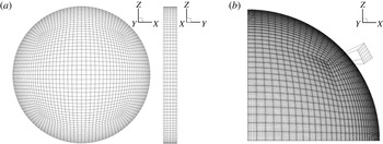
(a) Left: primary mesh on the vertical circular cross-section. There are in total 2700 primary elements on the cross-section. Right: primary mesh along the thickness direction. There are 6 primary mesh elements along the thickness direction. (b) A quarter section of the vertical circular cross-section. There are
 $8\times 8\times 8$
secondary nodes within each primary mesh for our DNS with polynomial order of 7.

The DNS is carried out in a vertical thin disk, which has the same geometry and dimensions as those used in the experiment. The corresponding non-dimensional boundary conditions are
 $$\begin{eqnarray}\displaystyle & \displaystyle \hat{\boldsymbol{u}}|_{walls}=0, & \displaystyle\end{eqnarray}$$
 $$\begin{eqnarray}\displaystyle & \displaystyle \boldsymbol{n}\boldsymbol{\cdot }\unicode[STIX]{x1D735}\hat{T}|_{non\text{-}conducting\,\;walls}=0, & \displaystyle\end{eqnarray}$$
 $$\begin{eqnarray}\displaystyle & \displaystyle \hat{T}|_{bottom}=0.5, & \displaystyle\end{eqnarray}$$
 $$\begin{eqnarray}\displaystyle & \displaystyle \hat{T}|_{top}=-0.5. & \displaystyle\end{eqnarray}$$
The control parameters are fixed at
 $Ra=5\times 10^{9}$
,
 $Pr=4.4$
and
 $\unicode[STIX]{x1D6E4}=0.1$
. As shown in figure 2, we use a flexible unstructured mesh on the vertical circular cross-section to adapt to the convective flow.
The minimum primary mesh size near the solid boundary is set to be
 $0.00387D$
, which is approximately the measured thermal BL thickness
 $\unicode[STIX]{x1D6FF}$
in the corresponding experiment. The polynomial order within each mesh element is set to
 $N=7$
so that we have 8 grid points to resolve the thermal BLs with the minimum secondary mesh size of
 $0.000261D$
. In total, there are 16 200 primary mesh elements and approximately 8.3 million grid points. Additional DNS tests are conducted to verify that with this spatial solution the Grötzbach criterion (Grötzbach Reference Grötzbach1983) is satisfied across the whole body of the flow, and the statistical properties of the convective flow, such as the thermal dissipation rate and kinetic energy dissipation rate, converge at
 $N=7$
.
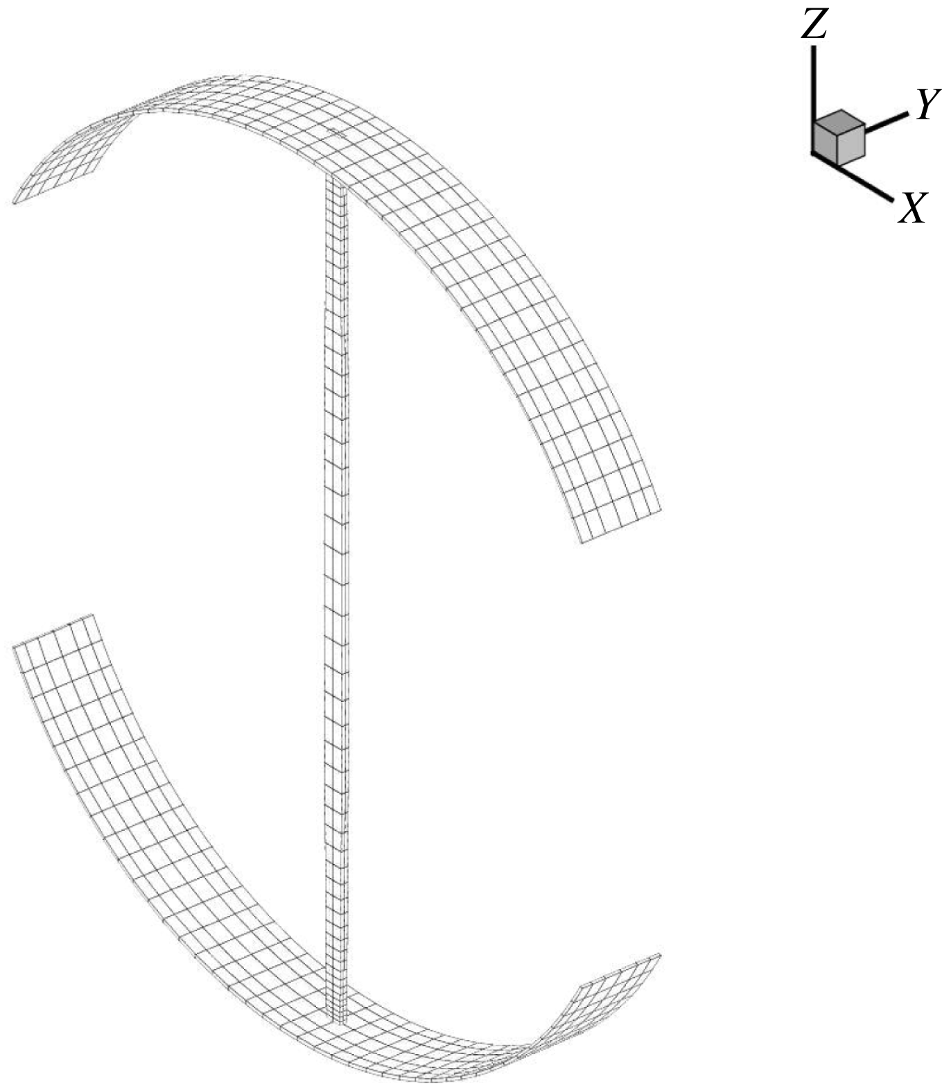
A thin column surrounding the vertical
 $z$
-axis used to calculate the time-averaged properties of the flow as a function of
 $z$
. The horizontal cross-section of the thin column has 4 primary elements and 256 nodes. Among the 256 nodes, the 24 closest nodes surrounding the
 $z$
-axis, which form a small area of
 $2.67\times 10^{-4}$
thickness square, are used to calculate the time-averaged properties of the flow.

Adaptive time steps are used to ensure the Courant number is below 0.5. During the simulation, the variable time step is approximately 0.0017 times the free-fall time. The DNS is run for 2600 free-fall times to reach a steady state, followed by a continuing evolution of another 5200 free-fall times in order to obtain the time series data of the velocity and temperature fields. The time-averaged properties of the flow along the vertical
 $z$
-axis, which will be presented below, are obtained in a narrow column surrounding the
 $z$
-axis, as shown in figure 3.
3 Numerical and experimental results
3.1 Direct numerical simulation results in the thin disk
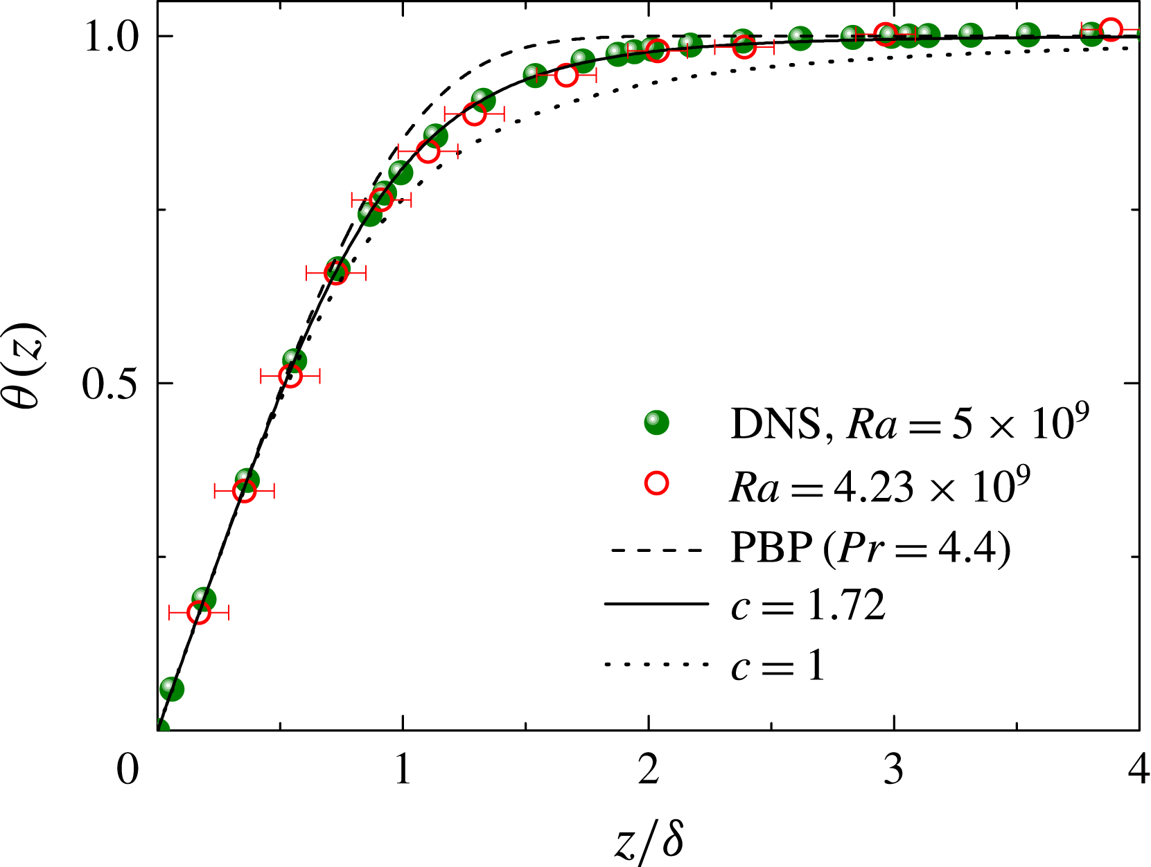
Numerically calculated mean temperature profile
 $\unicode[STIX]{x1D703}(z)$
(green solid circles) as a function of
 $z/\unicode[STIX]{x1D6FF}$
in the thin disk. Red open circles show the experimental data obtained at
 $Ra=4.23\times 10^{9}$
and
 $Pr=4.4$
(water). The error bars indicate the size of the thermistor bead used in the experiment. The solid and dotted lines are, respectively, the calculated
 $\unicode[STIX]{x1D703}(\unicode[STIX]{x1D709};c)$
using (1.3) with
 $c=1.72$
and
 $c=1$
. The dashed line shows the PBP profile for
 $Pr=4.4$
.

Figure 4 shows the numerically calculated mean temperature profile
 $\unicode[STIX]{x1D703}(z)$
(green solid circles) as a function of
 $z/\unicode[STIX]{x1D6FF}$
for
 $Pr=4.4$
. Here the BL thickness
 $\unicode[STIX]{x1D6FF}$
is defined as the distance at which the linear extrapolation of the mean temperature gradient at the bottom boundary intersects the mean temperature
 $T_{0}$
at the cell centre (Wang et al.
Reference Wang, He and Tong2016). The DNS results agree well with the experimental data (red open circles) obtained in the thin disk with
 $Pr=4.4$
(water). It has been shown (Wang et al.
Reference Wang, He and Tong2016) that the measured
 $\unicode[STIX]{x1D703}(z/\unicode[STIX]{x1D6FF})$
has a scaling form independent of
 $Ra$
in the
 $Ra$
range
 $1.5\times 10^{9}\lesssim Ra\lesssim 1.3\times 10^{10}$
. The two sets of data can be well described by the analytical solution (1.3) with the fitting parameter
 $c=1.72$
(solid line). The
 $c=1.72$
curve lies in between the
 $c=1$
curve (dotted line), which is the lowest value of
 $c$
allowed in the theory (Shishkina et al.
Reference Shishkina, Horn, Wagner and Ching2015), and the PBP profile for a laminar BL (with
 $c\rightarrow \infty$
, dashed line). The deviation of the
 $c=1.72$
curve from the PBP profile is clearly visible in the region
 $1<z/\unicode[STIX]{x1D6FF}<2$
with a smaller mean temperature gradient. As the total vertical heat flux in the system is a conserved quantity, a smaller mean temperature gradient corresponds to a larger convective heat flux (Ching, Dung & Shishkina Reference Ching, Dung and Shishkina2017). This finding thus suggests that BL fluctuations can enhance the convective heat transport.
The error bar of the experimental data points results mainly from the bead size of the thermistor used for the temperature measurement. The thermistor bead has a diameter of 0.17 mm and is coated with a thin layer of glass sealant. It is seen that, within the experimental uncertainties, the measured
 $\unicode[STIX]{x1D703}(z/\unicode[STIX]{x1D6FF})$
agrees well with the DNS results, suggesting that the small thermistor has a negligible effect on the measured mean temperature profile. We believe that the main effect of the thermistor size is to introduce a (spatial) running average over the measured
 $\unicode[STIX]{x1D703}(z/\unicode[STIX]{x1D6FF})$
, which only averages out small-scale fluctuations (comparable to the thermistor size) but does not affect the functional form of the smooth mean temperature profile.
(a) Numerically calculated temperature variance profile
 $\unicode[STIX]{x1D702}(z)/\unicode[STIX]{x1D702}_{0}$
(green solid circles) as a function of
 $z/\unicode[STIX]{x1D6FF}$
in the thin disk in a double-logarithmic plot. Red open circles show the experimental data obtained at
 $Ra=4.23\times 10^{9}$
. The vertical line indicates the transition distance
 $\unicode[STIX]{x1D709}_{c}\simeq 1.6$
. (b) Same data as in (a) but plotted on a linear scale for a clearer view of the fitting. The vertical error bars show the experimental uncertainties of the measurement. The solid curve is numerical solution
 $\unicode[STIX]{x1D6FA}(\unicode[STIX]{x1D709};c=1.72,\unicode[STIX]{x1D6E5}_{b}^{2}/\unicode[STIX]{x1D702}_{0}=46.3,d=1.4,\unicode[STIX]{x1D6FC}=1.15)$
of (1.5) with
 $\unicode[STIX]{x1D709}_{0}=0.816$
.

While the deviations of the measured/calculated
 $\unicode[STIX]{x1D703}(z)$
from the PBP form are clearly visible, they are nonetheless small and are only shown in the region
 $0.6\lesssim \unicode[STIX]{x1D709}\lesssim 2$
(Wang et al.
Reference Wang, He and Tong2016). The temperature variance profile
 $\unicode[STIX]{x1D702}(z)$
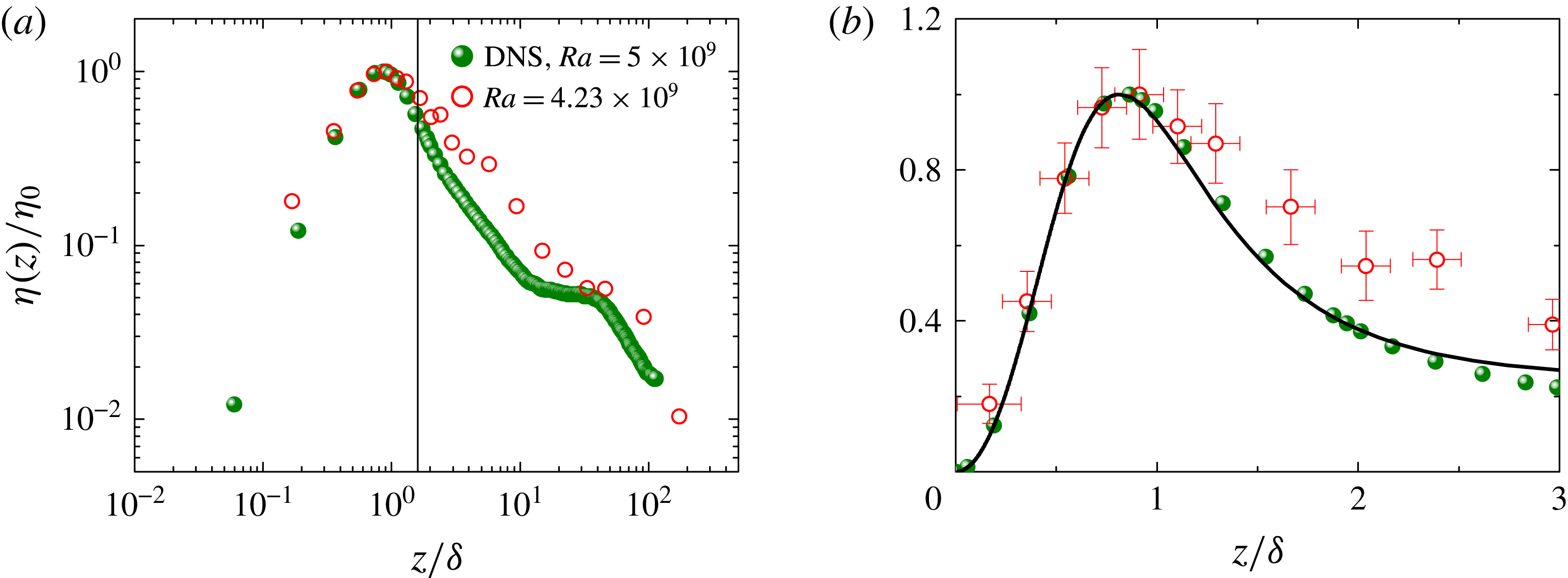
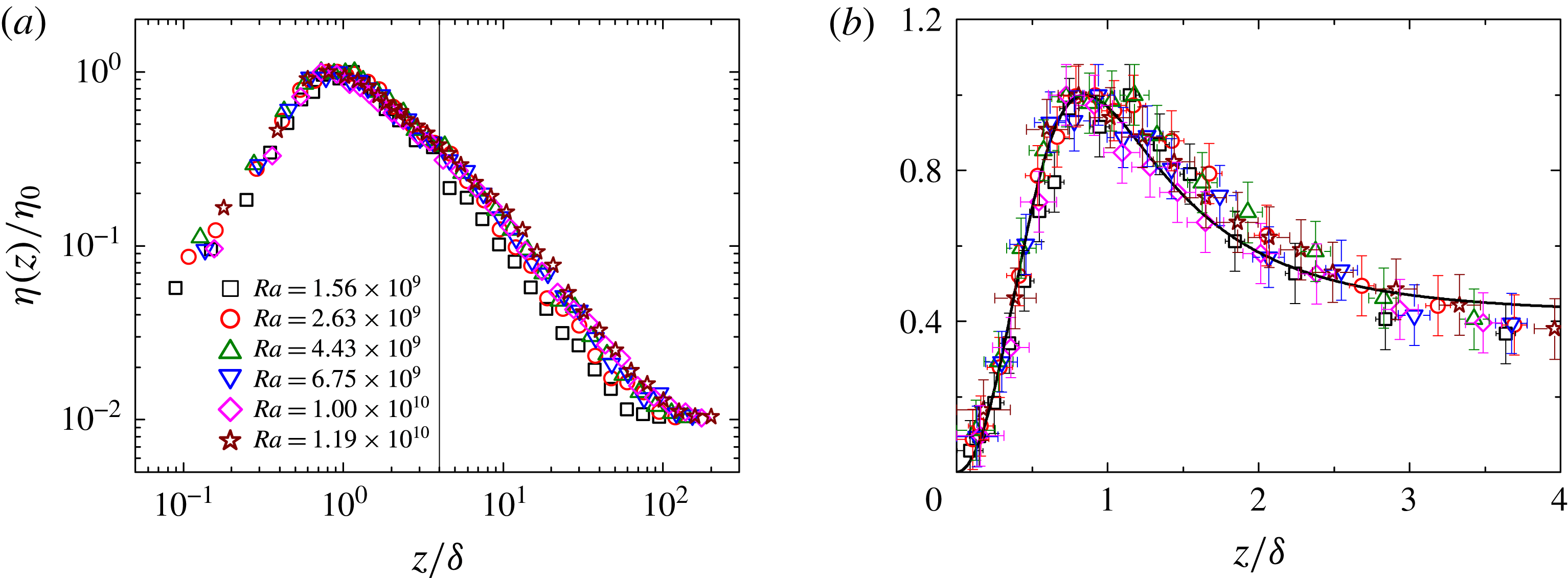
, on the other hand, is a direct measure of BL fluctuations and is absent in laminar BLs. Figure 5(a) shows a comparison between the numerically calculated temperature variance profile
 $\unicode[STIX]{x1D702}(z)/\unicode[STIX]{x1D702}_{0}$
(green solid circles) and the experimental data (open red circles) in a double-logarithmic plot. The two profiles collapse well in the region
 $z/\unicode[STIX]{x1D6FF}\lesssim \unicode[STIX]{x1D709}_{c}$
(vertical line) with
 $\unicode[STIX]{x1D709}_{c}\simeq 1.6$
being a transition distance, beyond which the measured
 $\unicode[STIX]{x1D702}(z)/\unicode[STIX]{x1D702}_{0}$
at different values of
 $Ra$
do not scale with the BL thickness
 $\unicode[STIX]{x1D6FF}$
any more (Wang et al.
Reference Wang, He and Tong2016). This value of
 $\unicode[STIX]{x1D709}_{c}$
is very close to the ratio of the viscous BL thickness
 $\unicode[STIX]{x1D6FF}_{\unicode[STIX]{x1D708}}$
to the thermal BL thickness
 $\unicode[STIX]{x1D6FF}$
for a laminar BL, i.e.
 $\unicode[STIX]{x1D709}_{c}\sim \unicode[STIX]{x1D6FF}_{\unicode[STIX]{x1D708}}/\unicode[STIX]{x1D6FF}=0.982Pr^{1/3}$
for
 $Pr>3$
(Stevens, Lohse & Verzicco Reference Stevens, Lohse and Verzicco2011; Shishkina, Horn & Wagner Reference Shishkina, Horn and Wagner2013).
To compare the DNS and experimental results more clearly, we plot, in figure 5(b), the same data as in figure 5(a) but on a linear scale with
 $\unicode[STIX]{x1D709}\leqslant 3$
. In the region
 $\unicode[STIX]{x1D709}\lesssim 1.5$
, the DNS and experimental results show good agreement. The solid line in figure 5(b) shows the numerical solution
 $\unicode[STIX]{x1D6FA}(\unicode[STIX]{x1D709};c=1.72,\unicode[STIX]{x1D6E5}_{b}^{2}/\unicode[STIX]{x1D702}_{0}=46.3,d=1.4,\unicode[STIX]{x1D6FC}=1.15)$
of (1.5), which is in excellent agreement with the DNS data. The horizontal error bar of the experimental data points is the same as that shown in figure 4, and the vertical error bar shows the experimental uncertainty of the measurement. Because temperature variance is a second-order quantity, it has relatively large experimental uncertainties. It is seen that there exist some differences between the experimental and DNS results for
 $\unicode[STIX]{x1D709}\gtrsim 1.5$
. One possible cause for the small deviations is that in the experiment the (bottom) conducting plate has small temperature fluctuations, which are absent in the DNS data. While the temperature variance of the bottom conducting plate has been subtracted out from the experimental data, it may still have some correlated influence on the bulk temperature fluctuations.
In addition to the comparison with the experimental data, the DNS results can also be used to directly check the assumptions made in the theoretical model, which are often difficult to obtain in the experiment. For example, from the DNS data one can calculate the cross-correlation functions
 $\langle v^{\prime }T^{\prime }\rangle$
and
 $\langle v^{\prime }{T^{\prime }}^{2}\rangle$
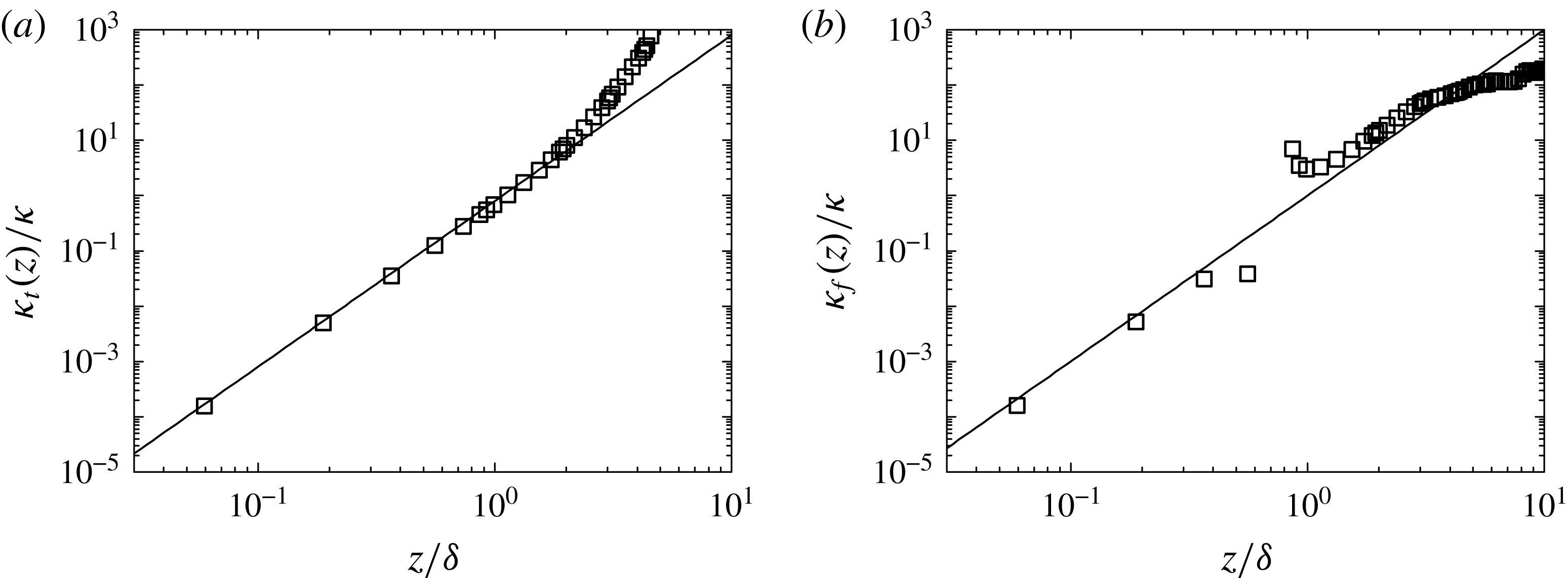
and test the validity of (1.2) and (1.7). Figure 6(a) shows the numerically calculated turbulent diffusivity
 $\unicode[STIX]{x1D705}_{t}/\unicode[STIX]{x1D705}$
for the mean temperature as a function of
 $z/\unicode[STIX]{x1D6FF}$
. The solid line shows a power-law fit
 $\unicode[STIX]{x1D705}_{t}/\unicode[STIX]{x1D705}=0.8\unicode[STIX]{x1D709}^{3}$
to the DNS data in the region
 $\unicode[STIX]{x1D709}\lesssim 2$
and thus (1.2) is confirmed within the thermal BL. Figure 6(b) shows the numerically calculated turbulent diffusivity
 $\unicode[STIX]{x1D705}_{f}/\unicode[STIX]{x1D705}$
for the temperature variance as a function of
 $z/\unicode[STIX]{x1D6FF}$
. The solid line shows a power-law fit
 $\unicode[STIX]{x1D705}_{f}/\unicode[STIX]{x1D705}=1.0\unicode[STIX]{x1D709}^{3}$
to the DNS data in the region
 $z/\unicode[STIX]{x1D6FF}\lesssim 3$
. There is a discontinuity at the peak position
 $\unicode[STIX]{x1D709}_{0}\simeq 0.8$
, at which
 $\unicode[STIX]{x2202}_{z}\unicode[STIX]{x1D702}(\unicode[STIX]{x1D709}_{0})=0$
, so that the error bar of the resulting
 $\unicode[STIX]{x1D705}_{f}$
increases significantly due to the lack of adequate grid points near this position. Except in this region, the DNS data can be well described by (1.7). In a recent DNS study, Shishkina et al. (Reference Shishkina, Horn, Wagner and Ching2015) calculated the turbulent diffusivity profile
 $\unicode[STIX]{x1D705}_{t}/\unicode[STIX]{x1D705}$
for the
 $\unicode[STIX]{x1D6E4}=1$
upright cylinder. While the two DNS studies were conducted under different conditions (thin disk versus upright cylinder and local profile versus cross-section-averaged profile), we find that in both convection systems the profile
 $\unicode[STIX]{x1D705}_{t}/\unicode[STIX]{x1D705}$
scales with
 $\unicode[STIX]{x1D709}^{3}$
and the proportionality constant
 $a$
for the cylinder (
 $a=1.76$
) is larger than that for the thin disk (
 $a=0.8$
). This is expected as the large-scale 3-D flow modes in the upright cylinder have more fluctuations outside the BL region and give rise to a larger value of
 $a$
, compared to the quasi-2-D flow in the thin disk (see more discussions on table 1 below).
(a) Numerically calculated turbulent diffusivity
 $\unicode[STIX]{x1D705}_{t}/\unicode[STIX]{x1D705}$
for the mean temperature as a function of
 $z/\unicode[STIX]{x1D6FF}$
in the thin disk. The solid line shows a power-law fit
 $\unicode[STIX]{x1D705}_{t}/\unicode[STIX]{x1D705}=0.8\unicode[STIX]{x1D709}^{3}$
. (b) Numerically calculated turbulent diffusivity
 $\unicode[STIX]{x1D705}_{f}/\unicode[STIX]{x1D705}$
for the temperature variance as a function of
 $z/\unicode[STIX]{x1D6FF}$
in the thin disk. The solid line shows a power-law fit
 $\unicode[STIX]{x1D705}_{f}/\unicode[STIX]{x1D705}=1.0\unicode[STIX]{x1D709}^{3}$
.

Fitted values of the parameters
 $c$
in (1.3) and
 $d$
and
 $\unicode[STIX]{x1D6FC}$
in the numerical solution
 $\unicode[STIX]{x1D6FA}(\unicode[STIX]{x1D709};c,\unicode[STIX]{x1D6E5}_{b}^{2}/\unicode[STIX]{x1D702}_{0},d,\unicode[STIX]{x1D6FC})$
of (1.5). The values of
 $a$
are calculated using (1.4) and fitted values of
 $c$
. The values of the peak position
 $\unicode[STIX]{x1D709}_{0}$
, transition distance
 $\unicode[STIX]{x1D709}_{c}$
, mixing zone exponent
 $\unicode[STIX]{x1D716}$
and the parameter
 $\unicode[STIX]{x1D6E5}_{b}^{2}/\unicode[STIX]{x1D702}_{0}$
are obtained directly from the experimental and DNS data.

With the DNS data one can also calculate the five individual contributions to the total variance (also called the budget terms), as marked in (1.5), using the original convective thermal equation for
 $\unicode[STIX]{x1D702}/\unicode[STIX]{x1D702}_{0}$
:
 $$\begin{eqnarray}\underbrace{-(\langle u\rangle \unicode[STIX]{x2202}_{x}\unicode[STIX]{x1D702}+\langle v\rangle \unicode[STIX]{x2202}_{z}\unicode[STIX]{x1D702})}_{mean\,convection}\overbrace{-\unicode[STIX]{x2202}_{z}\langle v^{\prime }{T^{\prime }}^{2}\rangle }^{turbulent\,convection}\underbrace{-2\langle v^{\prime }T^{\prime }\rangle \unicode[STIX]{x2202}_{z}\langle T\rangle }_{production}+\overbrace{\unicode[STIX]{x1D705}\unicode[STIX]{x2202}_{z}^{2}\unicode[STIX]{x1D702}}^{diffusion}\underbrace{-2\unicode[STIX]{x1D705}\langle (\unicode[STIX]{x1D735}T^{\prime })^{2}\rangle }_{thermal\,dissipation}=0,\end{eqnarray}$$
where
 $\langle u\rangle$
and
 $\langle v\rangle$
are the mean horizontal and vertical velocities. In addition,
 $\unicode[STIX]{x1D735}=\boldsymbol{e}_{x}\unicode[STIX]{x2202}_{x}+\boldsymbol{e}_{z}\unicode[STIX]{x2202}_{z}$
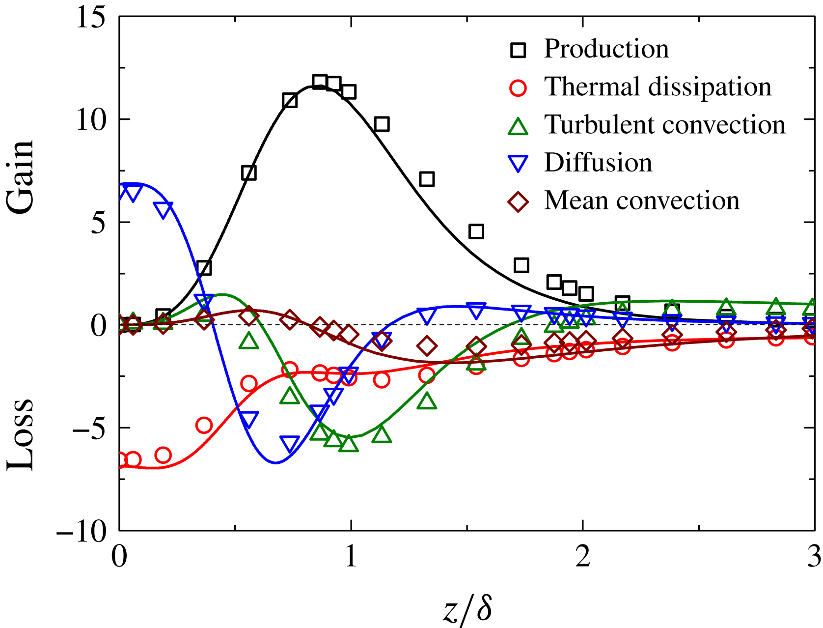
is the 2-D gradient operator. Figure 7 shows a comparison between the calculated budget terms using the DNS data in the thin disk (open symbols) and those obtained using the solution
 $\unicode[STIX]{x1D6FA}(\unicode[STIX]{x1D709};1.72,46.3,1.4,1.15)$
of (1.5) with
 $\unicode[STIX]{x1D709}_{0}=0.816$
(solid lines). Excellent agreement between the DNS data and theoretical model given in (1.5) is observed. Note that from the thermal dissipation term in (1.5), one can readily find that its first-order derivative equals to zero at
 $\unicode[STIX]{x1D709}_{0}=0.816$
. Indeed, the open circles show a local maximum at the peak position
 $\unicode[STIX]{x1D709}_{0}$
. These numerical results thus further confirm that our model shown in (1.5) captures the essential physics.
Comparison between the calculated budget terms using the DNS data in the thin disk (open symbols) and those obtained using the solution
 $\unicode[STIX]{x1D6FA}(\unicode[STIX]{x1D709};c=1.72,\unicode[STIX]{x1D6E5}_{b}^{2}/\unicode[STIX]{x1D702}_{0}=46.3,d=1.4,\unicode[STIX]{x1D6FC}=1.15)$
of (1.5) with maximum position
 $\unicode[STIX]{x1D709}_{0}=0.816$
(solid lines). All the budget terms are normalized by
 $\unicode[STIX]{x1D705}\unicode[STIX]{x1D702}_{0}/\unicode[STIX]{x1D6FF}^{2}$
.

(a) Measured mean temperature profile
 $\unicode[STIX]{x1D703}(z)$
as a function of
 $z/\unicode[STIX]{x1D6FF}$
for different values of
 $Ra$
and at fixed
 $Pr=4.4$
(water) in the upright cylinder. The measurements are made along the central axis of the cell near its bottom plate. The error bars indicate the size of the thermistor bead used. The solid and dotted lines are, respectively, the calculated
 $\unicode[STIX]{x1D703}(\unicode[STIX]{x1D709};c)$
using (1.3) with
 $c=1.2$
and
 $c=1$
. The dashed line shows the PBP profile for
 $Pr=4.4$
. (b) Measured
 $\unicode[STIX]{x1D703}(z)$
as a function of
 $z/\unicode[STIX]{x1D6FF}$
for different values of
 $Ra$
and at fixed
 $Pr=7.6$
(20 wt.% aqueous solution of glycerine). The solid and dotted lines are, respectively, the calculated
 $\unicode[STIX]{x1D703}(\unicode[STIX]{x1D709};c)$
using (1.3) with
 $c=1.3$
and
 $c=1$
. The dashed line shows the PBP profile for
 $Pr=7.6$
.

3.2 Experimental results in the upright cylinder
We now examine the measured mean temperature profile
 $\unicode[STIX]{x1D703}(z)$
and normalized temperature variance profile
 $\unicode[STIX]{x1D702}(z)/\unicode[STIX]{x1D702}_{0}$
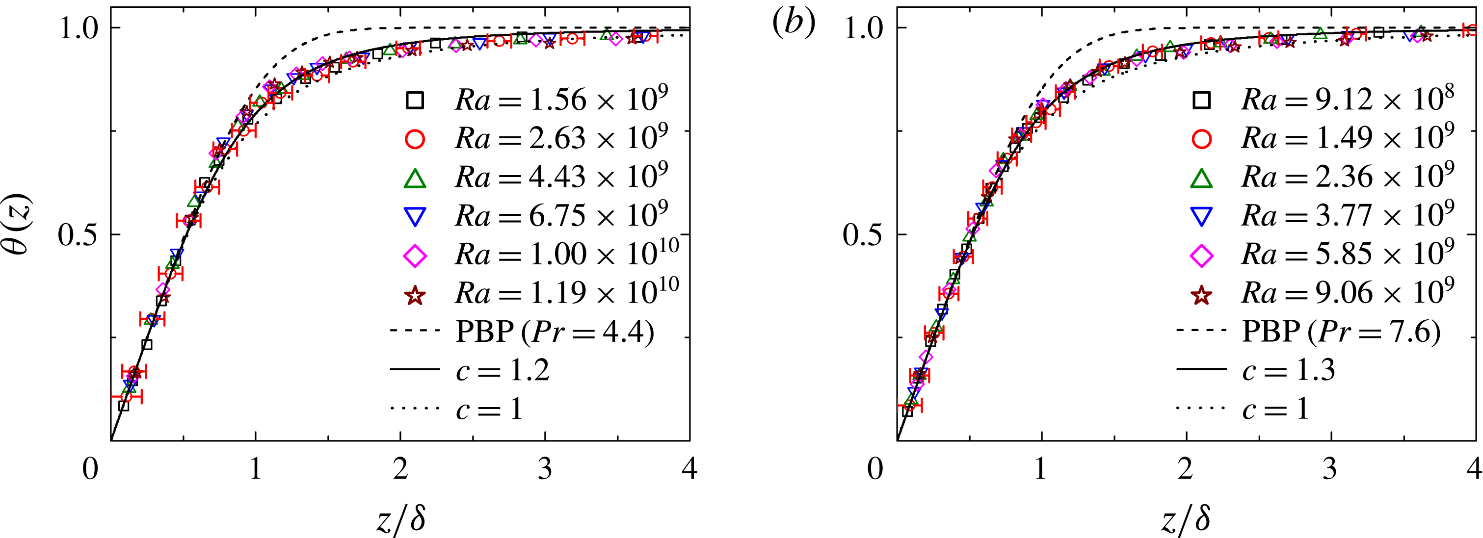
in the upright cylinder, in which the flow field has complex 3-D structures (Scheel & Schumacher Reference Scheel and Schumacher2014). Figure 8(a) shows the measured
 $\unicode[STIX]{x1D703}(z)$
as a function of
 $z/\unicode[STIX]{x1D6FF}$
for different values of
 $Ra$
and at fixed
 $Pr=4.4$
(water). All of the measured
 $\unicode[STIX]{x1D703}(z/\unicode[STIX]{x1D6FF})$
curves in the
 $Ra$
range studied collapse onto a single master curve, which can be well described by the calculated
 $\unicode[STIX]{x1D703}(\unicode[STIX]{x1D709};c)$
using (1.3) with the fitting parameter
 $c=1.2$
(solid line). Similarly, figure 8(b) shows the measured
 $\unicode[STIX]{x1D703}(z)$
as a function of
 $z/\unicode[STIX]{x1D6FF}$
for different values of
 $Ra$
and at fixed
 $Pr=7.6$
(20 wt.% aqueous solution of glycerine). The measured
 $\unicode[STIX]{x1D703}(z/\unicode[STIX]{x1D6FF})$
is also found to be well described by (1.3) with the fitting parameter
 $c=1.3$
(solid line), which deviates from the PBP form (dashed line) in the region
 $0.6\lesssim \unicode[STIX]{x1D709}\lesssim 3$
. Such deviations from the PBP form have been reported previously in the experiments for both
 $Pr>1$
(Lui & Xia Reference Lui and Xia1998; Du & Tong Reference Du and Tong2000) and
 $Pr<1$
(Du Puits, Resagk & Thess Reference Du Puits, Resagk and Thess2013) and in the DNS studies (Shishkina & Thess Reference Shishkina and Thess2009; Scheel, Kim & White Reference Scheel, Kim and White2012; Shi, Emran & Schumacher Reference Shi, Emran and Schumacher2012; Stevens et al.
Reference Stevens, Zhou, Grossmann, Verzicco, Xia and Lohse2012).
Measured thermal BL thickness
 $\unicode[STIX]{x1D6FF}$
as a function of
 $Ra$
in the thin disk (black squares) and
 $\unicode[STIX]{x1D6E4}=1$
upright cylinder (red circles) at a fixed value of
 $Pr=4.4$
(water). The error bars show the experimental uncertainties of the measurement. The solid and dashed lines are the power-law fits,
 $\unicode[STIX]{x1D6FF}=ARa^{\unicode[STIX]{x1D70F}}$
, to the data with
 $A=510~\text{mm}$
,
 $\unicode[STIX]{x1D70F}=-0.31\pm 0.03$
(solid line) and
 $A=440~\text{mm}$
,
 $\unicode[STIX]{x1D70F}=-0.29\pm 0.03$
(dashed line).

It is seen from figure 8 that plots of
 $\unicode[STIX]{x1D703}(z)$
versus
 $z/\unicode[STIX]{x1D6FF}$
remain unchanged in the
 $Ra$
range studied and only
 $\unicode[STIX]{x1D6FF}$
changes with
 $Ra$
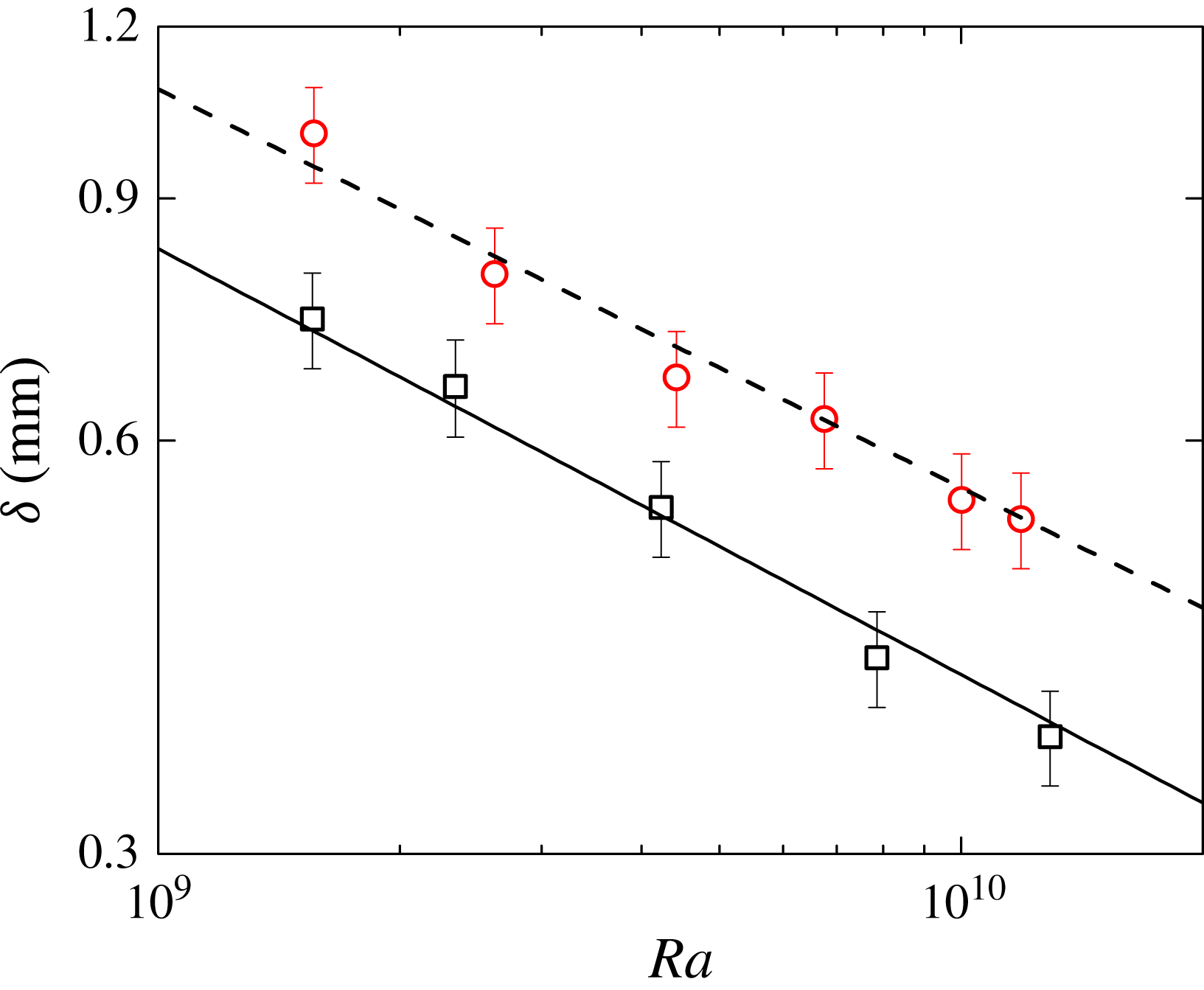
. Figure 9 shows the measured
 $\unicode[STIX]{x1D6FF}$
as a function of
 $Ra$
in the thin disk (black squares) and
 $\unicode[STIX]{x1D6E4}=1$
upright cylinder (red circles). Here
 $\unicode[STIX]{x1D6FF}$
is determined by the distance at which the tangent of the measured mean temperature profile
 $\langle T(z)\rangle$
near the conducting plate intersects the bulk fluid temperature (Wang et al.
Reference Wang, He and Tong2016). The data in the two convection cells can be well described by a power law,
 $\unicode[STIX]{x1D6FF}\sim Ra^{\unicode[STIX]{x1D70F}}$
, with
 $\unicode[STIX]{x1D70F}=-0.31\pm 0.03$
for the thin disk (solid line) and
 $\unicode[STIX]{x1D70F}=-0.29\pm 0.03$
for the upright cylinder (dashed line). The obtained value of
 $\unicode[STIX]{x1D70F}$
for the upright cylinder agrees with the previous measurement by Lui & Xia (Reference Lui and Xia1998). In the thin disk, we also measured the Nusselt number
 $Nu$
(dimensionless heat flux) as a function of
 $Ra$
for water (
 $Pr=4.4$
) and found that the measured
 $Nu$
is well described by the power law
 $Nu\sim Ra^{0.275\pm 0.03}$
(Wang et al.
Reference Wang, He and Tong2016; Wang Reference Wang2017). As
 $Nu\sim D/2\unicode[STIX]{x1D6FF}$
(Castaing et al.
Reference Castaing, Gunaratne, Heslot, Kadanoff, Libchaber, Thomae, Wu, Zaleski and Zanetti1989), the obtained value of
 $\unicode[STIX]{x1D70F}$
in the thin disk is thus consistent with the measured power-law exponent for
 $Nu$
.
Note that the
 $Ra$
-scaling of the measured
 $\unicode[STIX]{x1D703}(z/\unicode[STIX]{x1D6FF})$
, as shown in figure 8, is obtained in a fixed
 $\unicode[STIX]{x1D6E4}=1$
cylindrical cell for the
 $Pr>1$
fluids in the
 $Ra$
range,
 $8\times 10^{8}\lesssim Ra\lesssim 1.3\times 10^{10}$
. Such a
 $Ra$
-scaling was also observed in a fixed vertical thin disk under similar conditions (Wang et al.
Reference Wang, He and Tong2016). As shown in (1.3), the measured
 $\unicode[STIX]{x1D703}(z/\unicode[STIX]{x1D6FF})$
in figure 8 is normalized by the actual temperature difference
 $\unicode[STIX]{x1D6E5}_{b}\equiv T_{b}-T_{0}$
across the BL, instead of one half of the temperature difference
 $\unicode[STIX]{x0394}T/2$
across the entire cell. It was found by Wu & Libchaber (Reference Wu and Libchaber1991), Zhang, Childress & Libchaber (Reference Zhang, Childress and Libchaber1997) and Ahlers et al. (Reference Ahlers, Brown, Araujo, Funfschilling, Grossmann and Lohse2006) that the ratio
 $2\unicode[STIX]{x1D6E5}_{b}/\unicode[STIX]{x0394}T$
is not equal to unity and the deviation increases with
 $\unicode[STIX]{x0394}T$
for (most) fluids with the non-Boussinesq effect. We find that the
 $Ra$
-scaling of the measured
 $\unicode[STIX]{x1D703}(z/\unicode[STIX]{x1D6FF})$
is no longer valid if
 $\unicode[STIX]{x0394}T/2$
is used for normalization. The theoretical prediction given in (1.3) was obtained by assuming that the thermal BL is nested inside the velocity BL, so that it only applies to the
 $Pr>1$
fluids. For the
 $Pr<1$
fluids, the velocity BL is thinner than the thermal BL, which will introduce a new length scale to the problem in addition to the thermal BL thickness
 $\unicode[STIX]{x1D6FF}$
. As a result, the thermal BL becomes very sensitive to the large-scale flow inside the convection cell. Recent DNS studies (Shi et al.
Reference Shi, Emran and Schumacher2012; Scheel et al.
Reference Scheel, Kim and White2012; Stevens et al.
Reference Stevens, Zhou, Grossmann, Verzicco, Xia and Lohse2012; Schumacher, Götzfried & Scheel Reference Schumacher, Götzfried and Scheel2015) showed that the LSC changes sensitively with
 $Pr$
when
 $Pr<1$
. Indeed, the measured and numerically calculated mean temperature profiles
 $\unicode[STIX]{x1D703}(z/\unicode[STIX]{x1D6FF})$
for the
 $Pr<1$
fluids revealed larger deviations from the PBP form and the data do not always collapse onto a single master curve over a wider range of
 $Ra$
(see also Belmonte, Tilgner & Libchaber Reference Belmonte, Tilgner and Libchaber1993; Scheel et al.
Reference Scheel, Kim and White2012; Shi et al.
Reference Shi, Emran and Schumacher2012; Stevens et al.
Reference Stevens, Zhou, Grossmann, Verzicco, Xia and Lohse2012; Du Puits et al.
Reference Du Puits, Resagk and Thess2013; Shishkina et al.
Reference Shishkina, Horn, Wagner and Ching2017).
An important consideration when choosing the vertical thin disk and slightly tilted
 $\unicode[STIX]{x1D6E4}=1$
cylindrical cell in the experiment is that the LSC in the two cells is stable and can provide a simple uniform shear flow to the thermal BL in the
 $Ra$
range studied (Qiu & Tong Reference Qiu and Tong2001; Ahlers et al.
Reference Ahlers, Brown and Nikolaenko2006; Song et al.
Reference Song, Brown, Hawkins and Tong2014). This condition on the LSC is presumed in the theoretical modelling of the thermal BL. For turbulent convection in upright cylinders with
 $\unicode[STIX]{x1D6E4}\neq 1$
and with different cell shapes, such as cubic and rectangular cells, the LSC does not fit the convection cell well and the secondary flow in the cell may affect the BL dynamics. In fact, it was found that the measured mean temperature profiles
 $\unicode[STIX]{x1D703}(z/\unicode[STIX]{x1D6FF})$
for different values of
 $Ra$
do not collapse onto a single master curve even for the
 $Pr>1$
fluids in cubic and rectangular cells (Wang & Xia Reference Wang and Xia2003; Zhou & Xia Reference Zhou and Xia2013) and in
 $\unicode[STIX]{x1D6E4}\not =1$
upright cylinders (Lui & Xia Reference Lui and Xia1998). We speculate that the mismatch between the LSC and cell geometry and the resulting secondary flows may play an important role in the absence of scaling behaviour of the measured mean temperature profiles with
 $Ra$
. Evidently, the absence of scaling behaviour of the measured
 $\unicode[STIX]{x1D703}(z/\unicode[STIX]{x1D6FF})$
in the larger parameter space not covered in the present experiment is an unsettled issue and further study is needed.
(a) Measured temperature variance profile
 $\unicode[STIX]{x1D702}(z)/\unicode[STIX]{x1D702}_{0}$
as a function of
 $z/\unicode[STIX]{x1D6FF}$
in a double-logarithmic plot. The measurements are taken in the upright cylinder at different values of
 $Ra$
and at fixed
 $Pr=4.4$
(water). The vertical line indicates the transition distance
 $\unicode[STIX]{x1D709}_{c}=4$
. (b) Same data as in (a) but plotted on a linear scale for a clearer view of the fitting. The error bars show the experimental uncertainties of the measurement. The solid curve is the numerical solution
 $\unicode[STIX]{x1D6FA}(\unicode[STIX]{x1D709};1.2,25.4,2.1,0.91)$
of (1.5) with
 $\unicode[STIX]{x1D709}_{0}=0.85$
.

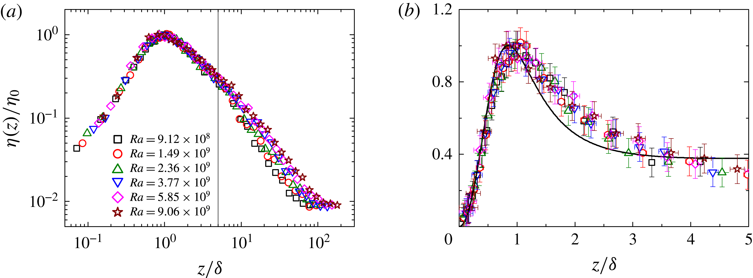
Figure 10(a) shows the measured
 $\unicode[STIX]{x1D702}(z)$
as a function of distance
 $z$
for different values of
 $Ra$
and at fixed
 $Pr=4.4$
(water) in the upright cylinder. In the plot,
 $\unicode[STIX]{x1D702}(z)$
is normalized by its maximal value
 $\unicode[STIX]{x1D702}_{0}$
and
 $z$
is normalized by
 $\unicode[STIX]{x1D6FF}$
. In the region
 $\unicode[STIX]{x1D709}\lesssim \unicode[STIX]{x1D709}_{c}\simeq 4$
, all the measured
 $\unicode[STIX]{x1D702}(z)/\unicode[STIX]{x1D702}_{0}$
curves collapse onto a single master curve, which has a single peak at
 $\unicode[STIX]{x1D709}_{0}\simeq 0.85$
. A similar single peaked
 $\unicode[STIX]{x1D702}(z)$
was also found previously in the upright cylinders (Belmonte et al.
Reference Belmonte, Tilgner and Libchaber1993; Belmonte, Tilgner & Libchaber Reference Belmonte, Tilgner and Libchaber1994; Lui & Xia Reference Lui and Xia1998; Du & Tong Reference Du and Tong2000; Du Puits et al.
Reference Du Puits, Resagk and Thess2013) and rectangular cells (Zhou & Xia Reference Zhou and Xia2013). Beyond
 $\unicode[STIX]{x1D709}\gtrsim \unicode[STIX]{x1D709}_{c}$
, the measured
 $\unicode[STIX]{x1D702}(z)/\unicode[STIX]{x1D702}_{0}$
no longer scales with
 $z/\unicode[STIX]{x1D6FF}$
. Instead, it scales with
 $z/H$
as shown in figure 13 below. To show the theoretical fitting more clearly, we plot, in figure 10(b), the same data as in figure 10(a) but on a linear scale with
 $\unicode[STIX]{x1D709}\leqslant 4$
. The solid line shows the numerical solution
 $\unicode[STIX]{x1D6FA}(\unicode[STIX]{x1D709};1.2,25.4,2.1,0.91)$
of (1.5) with
 $\unicode[STIX]{x1D709}_{0}=0.85$
, which is in excellent agreement with the experimental data.
(a) Measured temperature variance profile
 $\unicode[STIX]{x1D702}(z)/\unicode[STIX]{x1D702}_{0}$
as a function of
 $z/\unicode[STIX]{x1D6FF}$
in a double-logarithmic plot. The measurements are made in the upright cylinder at different values of
 $Ra$
and at fixed
 $Pr=7.6$
(20 wt.% glycerine solution). The vertical line indicates the transition distance
 $\unicode[STIX]{x1D709}_{c}=5$
. (b) Same data as in (a) but plotted on a linear scale. The error bars show the experimental uncertainties of the measurement. The solid curve is the numerical solution
 $\unicode[STIX]{x1D6FA}(\unicode[STIX]{x1D709};1.3,30,1.55,1.28)$
of (1.5) with
 $\unicode[STIX]{x1D709}_{0}=0.85$
.

Similarly, figure 11(a) shows the measured
 $\unicode[STIX]{x1D702}(z)/\unicode[STIX]{x1D702}_{0}$
as a function of
 $z/\unicode[STIX]{x1D6FF}$
for
 $Pr=7.6$
(20 wt.% glycerine solution) in the upright cylinder. It is seen that the scaling behaviour of the temperature variance profiles remains only up to
 $\unicode[STIX]{x1D709}\leqslant \unicode[STIX]{x1D709}_{c}\simeq 5$
along the cell axis and there is a sharp transition to a new scaling regime (mixing zone) at
 $\unicode[STIX]{x1D709}_{c}\simeq 5$
, beyond which a different model is needed to describe the mean and variance temperature profiles (Castaing et al.
Reference Castaing, Gunaratne, Heslot, Kadanoff, Libchaber, Thomae, Wu, Zaleski and Zanetti1989; Adrian Reference Adrian1996). The value of
 $\unicode[STIX]{x1D709}_{c}$
is found to increase with
 $Pr$
, a trend which is also found in the thin disk (Wang et al.
Reference Wang, He and Tong2016). Figure 11(b) shows a comparison between the numerical solution
 $\unicode[STIX]{x1D6FA}(\unicode[STIX]{x1D709};1.3,30,1.55,1.28)$
of (1.5) with
 $\unicode[STIX]{x1D709}_{0}=0.85$
(solid line) and the measured
 $\unicode[STIX]{x1D702}(z)/\unicode[STIX]{x1D702}_{0}$
in the range
 $\unicode[STIX]{x1D709}\lesssim 5$
. Fairly good agreement is obtained between the theory and experimental data.
Measured thermal dissipation rate
 $\unicode[STIX]{x1D716}_{T}(z)\unicode[STIX]{x1D6FF}^{2}/(\unicode[STIX]{x1D705}\unicode[STIX]{x1D702}_{0})$
(squares) as a function of
 $z/\unicode[STIX]{x1D6FF}$
. The measurements were made at
 $Ra=3.9\times 10^{9}$
and
 $Pr=5.5$
in a
 $\unicode[STIX]{x1D6E4}=1$
upright cylinder (He & Tong Reference He and Tong2009). The solid curve shows the calculated dissipation profile using the numerical solution
 $\unicode[STIX]{x1D6FA}(\unicode[STIX]{x1D709};1.2,25.4,2.1,0.9)$
of (1.5) with
 $\unicode[STIX]{x1D709}_{0}=0.85$
for
 $Pr=4.4$
.

Measured temperature variance profile
 $\unicode[STIX]{x1D702}(z)/\unicode[STIX]{x1D702}_{0}$
as a function of
 $z/H$
for different values of
 $Ra$
in the upright cylinder. The measurements are made at a fixed value of (a)
 $Pr=4.4$
(water) and (b)
 $Pr=7.6$
(20 wt.% glycerine solution). The data are the same as those shown in figures 10(a) and 11(a). The vertical lines indicate the transition distances (a)
 $z_{c}/H\simeq 0.04$
and (b)
 $z_{c}/H\simeq 0.06$
. The solid lines show the power-law fits,
 $\unicode[STIX]{x1D702}/\unicode[STIX]{x1D702}_{0}\sim (z/H)^{\unicode[STIX]{x1D716}}$
, with (a)
 $\unicode[STIX]{x1D716}=-1.1$
and (b)
 $\unicode[STIX]{x1D716}=-1.15$
.

An important feature of (1.5) is that the temperature variance profile
 $\unicode[STIX]{x1D702}(z)$
is inherently connected to the thermal dissipation profile
 $\unicode[STIX]{x1D716}_{T}(z)\equiv \unicode[STIX]{x1D705}\langle (\unicode[STIX]{x1D735}T^{\prime })^{2}\rangle$
, as (1.5) serves as an energy-budget-like equation. Experimentally,
 $\unicode[STIX]{x1D702}(z)$
is relatively easier to measure compared to
 $\unicode[STIX]{x1D716}_{T}(z)$
and thus one can use (1.5) to calculate
 $\unicode[STIX]{x1D716}_{T}(\unicode[STIX]{x1D709})$
once
 $\unicode[STIX]{x1D6FA}(\unicode[STIX]{x1D709})$
is determined from the measured
 $\unicode[STIX]{x1D702}(z)$
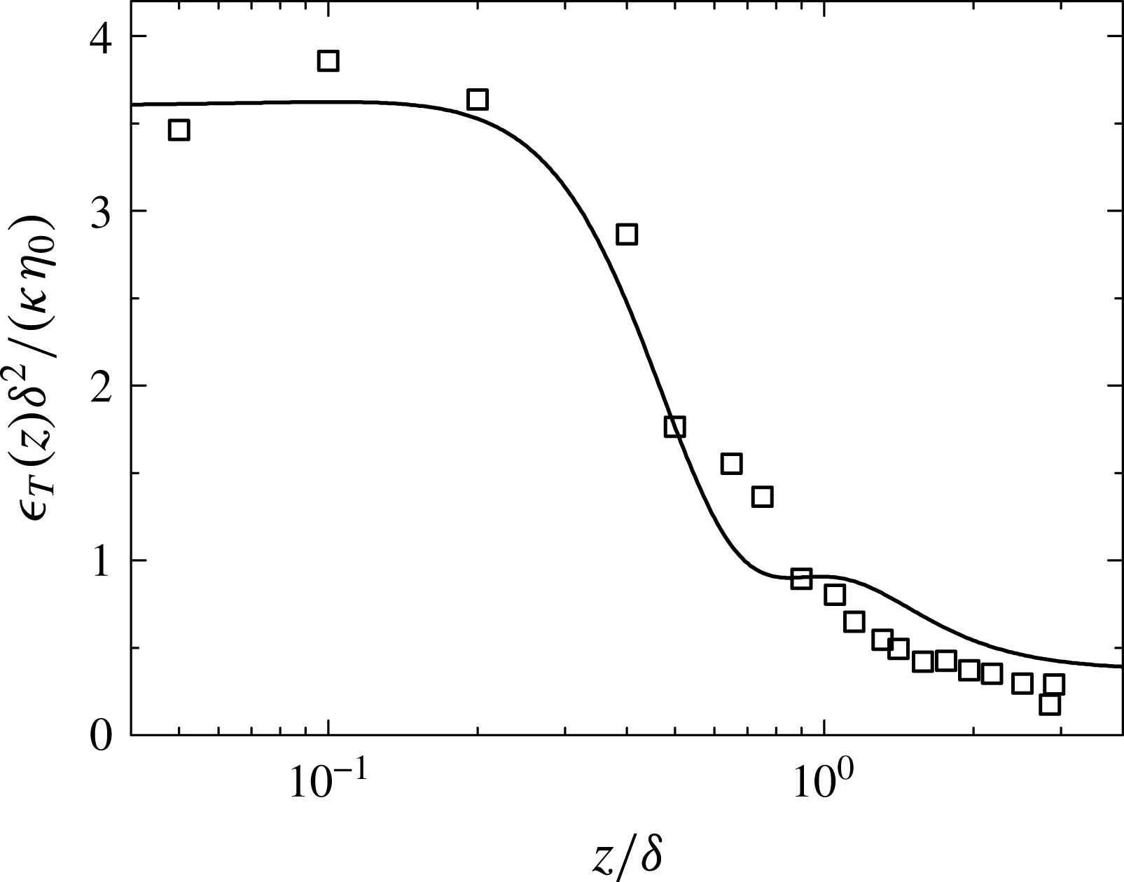
. Figure 12 shows a comparison between the calculated
 $\unicode[STIX]{x1D716}_{T}(z)$
using the numerical solution
 $\unicode[STIX]{x1D6FA}(\unicode[STIX]{x1D709};1.2,25.4,2.1,0.91)$
for
 $Pr=4.4$
and the previously measured
 $\unicode[STIX]{x1D716}_{T}(z)$
in a
 $\unicode[STIX]{x1D6E4}=1$
upright cylinder with
 $Pr=5.4$
(He & Tong Reference He and Tong2009). In the plot,
 $\unicode[STIX]{x1D716}_{T}(\unicode[STIX]{x1D709})$
is normalized by
 $\unicode[STIX]{x1D6FF}^{2}/(\unicode[STIX]{x1D705}\unicode[STIX]{x1D702}_{0})$
. Good agreement is obtained between the theory and experimental data in the BL region. The solid line in figure 12 has a plateau region near
 $\unicode[STIX]{x1D709}=\unicode[STIX]{x1D709}_{0}$
, which marks the position above which the contribution of the bulk flow to the thermal dissipation rate becomes dominant over the BL contribution (Wang et al.
Reference Wang, He and Tong2016). Figure 12 thus further confirms that (1.3) and (1.5) can be applied to other thermal BLs with different flow geometries.
Table 1 gives a summary of the fitted values of the parameters used in the solution of the mean temperature and temperature variance profiles. To explain the variations of the fitting parameter
 $c$
in a straightforward way, we convert the values of
 $c$
to the corresponding values of the dimensionless turbulent diffusivity coefficient
 $a$
using (1.4). The fitting results reveal a general trend that in the same convection cell, the level of BL fluctuations, as described by the turbulent diffusivity coefficients
 $a$
and
 $d$
and by the measured maximal value
 $\unicode[STIX]{x1D702}_{0}$
of the temperature variance (which is inversely proportional to the measured
 $\unicode[STIX]{x1D6E5}_{b}^{2}/\unicode[STIX]{x1D702}_{0}$
), decreases with increasing
 $Pr$
. This is because the enhanced viscous effect suppresses fluctuations of the thermal BL, which is nested underneath the viscous BL. Compared to the quasi-2-D flow in the thin disk, the 3-D large-scale flow in the upright cylinder has more fluctuations outside the BL region, resulting in larger BL fluctuations in the cylinder. On the other hand, the peak position
 $\unicode[STIX]{x1D709}_{0}$
of the temperature variance profiles is found to be a constant
 $\unicode[STIX]{x1D709}_{0}\simeq 0.80\pm 0.05$
, which does not change much with
 $Pr$
and cell shape. In table 1, the error bars for
 $\unicode[STIX]{x1D709}_{0}$
indicate the experimental uncertainties. For the DNS data, the error bar is one half of the mesh size. A similar value of
 $\unicode[STIX]{x1D709}_{0}$
was also obtained previously in a cubic cell filled with water (Wang & Xia Reference Wang and Xia2003; Zhou & Xia Reference Zhou and Xia2013). Similarly, the mean Taylor microscale
 $\ell$
in the thermal BL is determined primarily by the BL thickness
 $\unicode[STIX]{x1D6FF}$
, so that the ratio
 $\unicode[STIX]{x1D6FC}=\unicode[STIX]{x1D6FF}^{2}/\ell ^{2}$
is found to be a constant close to unity. Table 1 shows that the measured
 $\unicode[STIX]{x1D709}_{c}$
increases with
 $Pr$
, and it appears to scale with the ratio of the viscous BL thickness
 $\unicode[STIX]{x1D6FF}_{\unicode[STIX]{x1D708}}$
to the thermal BL thickness
 $\unicode[STIX]{x1D6FF}$
for a laminar BL, i.e.
 $\unicode[STIX]{x1D709}_{c}\sim \unicode[STIX]{x1D6FF}_{\unicode[STIX]{x1D708}}/\unicode[STIX]{x1D6FF}\sim Pr^{1/3}$
for
 $Pr>3$
(Stevens et al.
Reference Stevens, Lohse and Verzicco2011; Shishkina et al.
Reference Shishkina, Horn and Wagner2013).
3.3 Turbulent temperature fluctuations in the mixing zone
As mentioned above, when
 $\unicode[STIX]{x1D709}>\unicode[STIX]{x1D709}_{c}$
, the measured
 $\unicode[STIX]{x1D702}(z)/\unicode[STIX]{x1D702}_{0}$
does not scale with
 $z/\unicode[STIX]{x1D6FF}$
any more. We now examine the scaling behaviour of the temperature variance profile
 $\unicode[STIX]{x1D702}(z)$
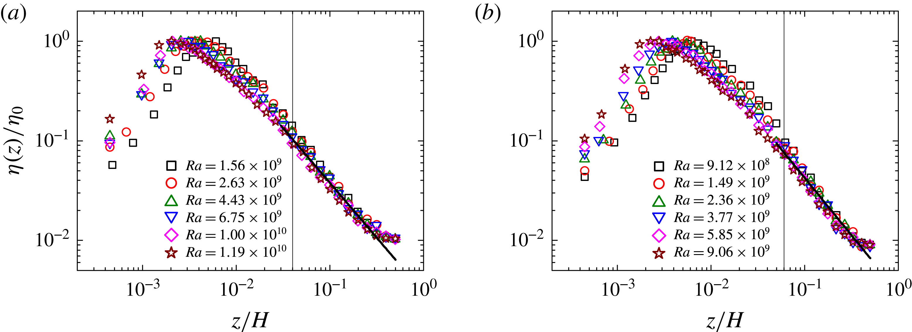
in this region. Figure 13 shows the measured
 $\unicode[STIX]{x1D702}(z)/\unicode[STIX]{x1D702}_{0}$
as a function of
 $z/H$
for different values of
 $Ra$
in the upright cylinder. It is seen that for both working fluids, the measured
 $\unicode[STIX]{x1D702}(z)/\unicode[STIX]{x1D702}_{0}$
remains approximately unchanged with
 $Ra$
and scales with
 $z/H$
in the region
 $0.06\lesssim z/H\lesssim 0.5$
. In particular, in the region
 $0.06\lesssim z/H\lesssim 0.4$
, the measured
 $\unicode[STIX]{x1D702}(z)/\unicode[STIX]{x1D702}_{0}$
can be described by a power law,
 $\unicode[STIX]{x1D702}/\unicode[STIX]{x1D702}_{0}\sim (z/H)^{\unicode[STIX]{x1D716}}$
with
 $\unicode[STIX]{x1D716}=-1.1\pm 0.1$
for
 $Pr=4.4$
(water) and
 $\unicode[STIX]{x1D716}=-1.15\pm 0.1$
for
 $Pr=7.6$
(20 wt.% glycerine solution). Here we call this region the mixing zone (Castaing et al.
Reference Castaing, Gunaratne, Heslot, Kadanoff, Libchaber, Thomae, Wu, Zaleski and Zanetti1989).
Measured temperature variance profile
 $\unicode[STIX]{x1D702}(z)/\unicode[STIX]{x1D702}_{0}$
(open symbols) as a function of
 $z/D$
for different values of
 $Ra$
and at fixed
 $Pr=4.4$
in the thin disk (Wang et al.
Reference Wang, He and Tong2016). Green solid circles show the calculated
 $\unicode[STIX]{x1D702}(z)/\unicode[STIX]{x1D702}_{0}$
using the DNS data along the central axis. The vertical line indicates the transition distance
 $z_{c}/D\simeq 0.01$
. The solid and dashed lines show the power-law fits,
 $\unicode[STIX]{x1D702}/\unicode[STIX]{x1D702}_{0}\sim (z/D)^{\unicode[STIX]{x1D716}}$
with
 $\unicode[STIX]{x1D716}=-0.9$
and
 $\unicode[STIX]{x1D716}=-0.98$
, respectively.

Similar scaling behaviour in the mixing zone is also found in the thin disk (Wang et al.
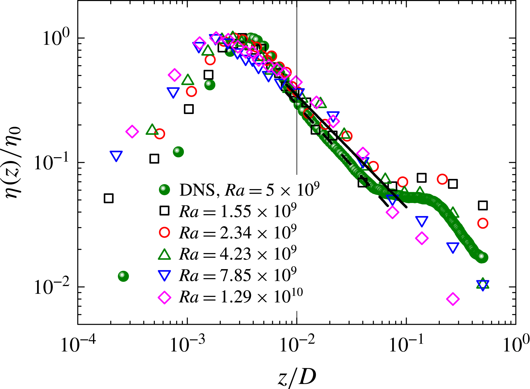
Reference Wang, He and Tong2016). Figure 14 shows the measured
 $\unicode[STIX]{x1D702}(z)/\unicode[STIX]{x1D702}_{0}$
(open symbols) as a function of
 $z/D$
for different values of
 $Ra$
and at fixed
 $Pr=4.4$
(water) in the thin disk. It is seen that the measured
 $\unicode[STIX]{x1D702}(z)/\unicode[STIX]{x1D702}_{0}$
remains approximately unchanged
 $Ra$
and scales with
 $z/D$
in the region
 $0.01\lesssim z/D\lesssim 0.1$
. Similar scaling behaviour was also reported for the 20 wt.% glycerine solution (
 $Pr=7.6$
) in the thin disk (Wang et al.
Reference Wang, He and Tong2016). In contrast to the upright cylinder, the upper bound of the mixing zone in the thin disk is limited to
 $z/D\simeq 0.1$
, beyond which the measured
 $\unicode[STIX]{x1D702}(z)/\unicode[STIX]{x1D702}_{0}$
do not scale with
 $z/D$
any more. This is because the convective flow in the mixing zone is truncated by the cell thickness
 $L/D\simeq 0.1$
. Similar to the upright cylinder, the measured
 $\unicode[STIX]{x1D702}(z)/\unicode[STIX]{x1D702}_{0}$
in the mixing zone of the thin disk can also be well described by the power law,
 $\unicode[STIX]{x1D702}/\unicode[STIX]{x1D702}_{0}\sim (z/D)^{\unicode[STIX]{x1D716}}$
with
 $\unicode[STIX]{x1D716}=-0.9\pm 0.1$
for both
 $Pr=4.4$
(water) and
 $Pr=7.6$
(20 wt.% glycerine solution), and
 $\unicode[STIX]{x1D716}=-0.98\pm 0.1$
for the DNS data.
4 Further theoretical analysis
(a) Calculated budget terms in (3.1) as a function of
 $z/D$
in the thin disk. The vertical line indicates the transition distance
 $z_{c}/D\simeq 0.025$
. (b) Calculated ratio
 $-\unicode[STIX]{x2202}_{z}\langle v^{\prime }{T^{\prime }}^{2}\rangle /2\unicode[STIX]{x1D716}_{T}$
as a function of
 $z/D$
in the thin disk. The horizontal lines indicate the condition
 $-\unicode[STIX]{x2202}_{z}\langle v^{\prime }{T^{\prime }}^{2}\rangle /2\unicode[STIX]{x1D716}_{T}=1\pm 0.1$
. The calculations in (a) and (b) are conducted using the DNS data and are averaged across the cell thickness
 $L$
.

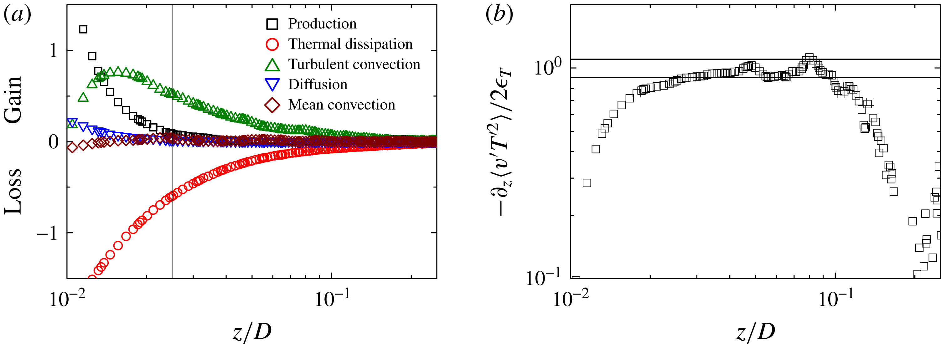
We first discuss the relative magnitude of each budget term in (3.1) in the mixing zone. Figure 15(a) shows the five budget terms as a function of
 $z/D$
along the central axis of the thin disk. The calculation is conducted using the DNS data and is averaged across the cell thickness
 $L$
. In the region
 $0.025\lesssim z/D\lesssim 0.1$
, there are only two dominant terms remaining, namely, the turbulent convection term
 $-\unicode[STIX]{x2202}_{z}\langle v^{\prime }{T^{\prime }}^{2}\rangle$
is balanced by the thermal dissipation term
 $2\unicode[STIX]{x1D716}_{T}$
, and the other three terms become negligibly small. To see this balance more clearly, we plot, in figure 15(b), the ratio of the two terms,
 $-\unicode[STIX]{x2202}_{z}\langle v^{\prime }{T^{\prime }}^{2}\rangle /2\unicode[STIX]{x1D716}_{T}$
, as a function of
 $z/D$
. It is seen that
 $-\unicode[STIX]{x2202}_{z}\langle v^{\prime }{T^{\prime }}^{2}\rangle /2\unicode[STIX]{x1D716}_{T}=1\pm 0.1$
in the region
 $0.25\lesssim z/D\lesssim 0.1$
, and thus the two terms maintain balance in this region.
Based on the above experimental and numerical findings, we now derive the equation of motion in the mixing zone. By taking Reynolds decomposition on the convective thermal equation, one finds (Wang et al. Reference Wang, He and Tong2016)
 $$\begin{eqnarray}\langle \boldsymbol{V}\rangle \boldsymbol{\cdot }\unicode[STIX]{x1D735}\unicode[STIX]{x1D702}+2\langle \boldsymbol{V}^{\prime }T^{\prime }\rangle \boldsymbol{\cdot }\unicode[STIX]{x1D735}\langle T\rangle +\unicode[STIX]{x1D735}\boldsymbol{\cdot }\langle \boldsymbol{V}^{\prime }{T^{\prime }}^{2}\rangle =\unicode[STIX]{x1D705}\unicode[STIX]{x1D6FB}^{2}\unicode[STIX]{x1D702}-2\unicode[STIX]{x1D716}_{T},\end{eqnarray}$$
where
 $\boldsymbol{V}=u(x,z)\boldsymbol{e}_{x}+v(x,z)\boldsymbol{e}_{z}$
is the velocity field (see figure 1 for the coordinate system used) and
 $\boldsymbol{V}^{\prime }\equiv \boldsymbol{V}-\langle \boldsymbol{V}\rangle$
is its fluctuation. To obtain (4.1), we have assumed
 $\unicode[STIX]{x2202}_{t}\unicode[STIX]{x1D702}=0$
for a steady-state flow and
 $\unicode[STIX]{x1D735}\boldsymbol{\cdot }\boldsymbol{V}=\unicode[STIX]{x1D735}\boldsymbol{\cdot }\boldsymbol{V}^{\prime }=0$
for an incompressible fluid. The five terms in (4.1) have the same meaning as those marked in (3.1). After taking an average across the cell thickness
 $L$
, the remaining large-scale flow inside the cell has a dominant circular component in the circular cross-section of the thin disk. This implies that the mean velocity
 $\langle \boldsymbol{V}\rangle$
only has an
 $x$
-component along the central axis. In addition, due to the rotational symmetry of the LSC, the velocity and temperature fields along the central axis have a much weaker
 $x$
-dependence than the
 $z$
-dependence. Combining these two characteristics, one has
 $\unicode[STIX]{x2202}_{x}\simeq 0$
,
 $\unicode[STIX]{x2202}_{x}^{2}\simeq 0$
and
 $\langle u\rangle \unicode[STIX]{x2202}_{x}+\langle v\rangle \unicode[STIX]{x2202}_{z}\simeq 0$
. Similar approximations were also made for turbulent channel flows (Pope Reference Pope2000). Under these approximations and noting that the mean temperature
 $\langle T\rangle$
in the mixing zone has a much weaker
 $z$
-dependence (see figure 4), we find (4.1) can be reduced to
 $$\begin{eqnarray}\unicode[STIX]{x2202}_{z}\langle v^{\prime }{T^{\prime }}^{2}\rangle \simeq \unicode[STIX]{x1D705}\unicode[STIX]{x2202}_{z}^{2}\unicode[STIX]{x1D702}-2\unicode[STIX]{x1D716}_{T},\end{eqnarray}$$
where the thermal dissipation rate takes the form (Wang et al. Reference Wang, He and Tong2016)
 $$\begin{eqnarray}\unicode[STIX]{x1D716}_{T}\simeq \unicode[STIX]{x1D705}\left[\frac{1}{4}\frac{(\unicode[STIX]{x2202}_{z}\unicode[STIX]{x1D702})^{2}}{\unicode[STIX]{x1D702}}+\frac{\unicode[STIX]{x1D702}}{\ell ^{2}}\right],\end{eqnarray}$$
with
 $\ell (z)$
being the Taylor microscale.
As shown in figures 10(a), 11(a) and 13, the characteristic length in the mixing zone is no longer the BL thickness
 $\unicode[STIX]{x1D6FF}$
, instead, the measured
 $\unicode[STIX]{x1D702}(z)/\unicode[STIX]{x1D702}_{0}$
is found to scale with the cell height
 $H$
(for the upright cylinder) or the cell thickness
 $L$
(for the thin disk). As a result, we expect
 $\unicode[STIX]{x2202}_{z}\lesssim 1/L$
. On the other hand, table 1 shows that the fitted values of
 $\unicode[STIX]{x1D6FC}\equiv \unicode[STIX]{x1D6FF}^{2}/\ell ^{2}\simeq 1$
, indicating that the Taylor microscale
 $\ell \simeq \unicode[STIX]{x1D6FF}$
. This is because even in the mixing zone, the spatial correlation of temperature fluctuations is produced primarily by the thermal plumes, which have a characteristic length comparable to
 $\unicode[STIX]{x1D6FF}$
. Because the length ratios
 $(L/\unicode[STIX]{x1D6FF})^{2}\simeq 400$
(for the thin disk) and
 $(H/\unicode[STIX]{x1D6FF})^{2}\simeq 40\,000$
(for the upright cylinder), the terms
 $\unicode[STIX]{x1D705}\unicode[STIX]{x2202}_{z}^{2}\unicode[STIX]{x1D702}$
in (4.2) and
 $\unicode[STIX]{x1D705}(\unicode[STIX]{x2202}_{z}\unicode[STIX]{x1D702})^{2}/(4\unicode[STIX]{x1D702})$
in (4.3) are negligibly small. Therefore, equations (4.2) and (4.3) can be further reduced to
 $$\begin{eqnarray}\unicode[STIX]{x2202}_{z}\langle v^{\prime }{T^{\prime }}^{2}\rangle =-2\unicode[STIX]{x1D716}_{T},\end{eqnarray}$$
with
 $\unicode[STIX]{x1D716}_{T}\simeq \unicode[STIX]{x1D705}\unicode[STIX]{x1D702}/\ell ^{2}$
. Equation (4.4) thus provides a clearer picture of the dynamics in the mixing zone compared with the previous models (Castaing et al.
Reference Castaing, Gunaratne, Heslot, Kadanoff, Libchaber, Thomae, Wu, Zaleski and Zanetti1989; Adrian Reference Adrian1996) and is fully supported by the DNS results as shown in figure 15(a). A close analogy to (4.4) is the kinetic energy equation for turbulent channel flows, in which the production and dissipation of the kinetic energy are in balance (Pope Reference Pope2000).
To solve (4.4), we assume that in the mixing zone the thermal plumes have a typical temperature fluctuation
 $T_{c}\sim \unicode[STIX]{x1D702}^{1/2}(z)$
and a typical free-fall velocity
 $u_{c}\sim (\unicode[STIX]{x1D6FC}gT_{c}\ell _{c})^{1/2}$
at a distance
 $\ell _{c}\sim z$
, which is the size of the largest eddy that the flow can excite (Townsend Reference Townsend1976). In this case, one has
 $\unicode[STIX]{x2202}_{z}\unicode[STIX]{x1D702}\simeq -\unicode[STIX]{x1D702}/\ell _{c}$
,
 $\langle v^{\prime }{T^{\prime }}^{2}\rangle \simeq u_{c}\unicode[STIX]{x1D702}$
and
 $\unicode[STIX]{x2202}_{z}\langle v^{\prime }{T^{\prime }}^{2}\rangle \simeq -u_{c}\unicode[STIX]{x1D702}/l_{c}$
, where the minus sign is introduced to indicate that the temperature variance is a decaying function of
 $z/D$
. With these equations, we find
 $$\begin{eqnarray}\unicode[STIX]{x1D705}_{f}\simeq u_{c}\ell _{c}\simeq a_{1}(\unicode[STIX]{x1D6FC}g)^{1/2}z^{3/2}\unicode[STIX]{x1D702}^{1/4},\end{eqnarray}$$
where
 $a_{1}$
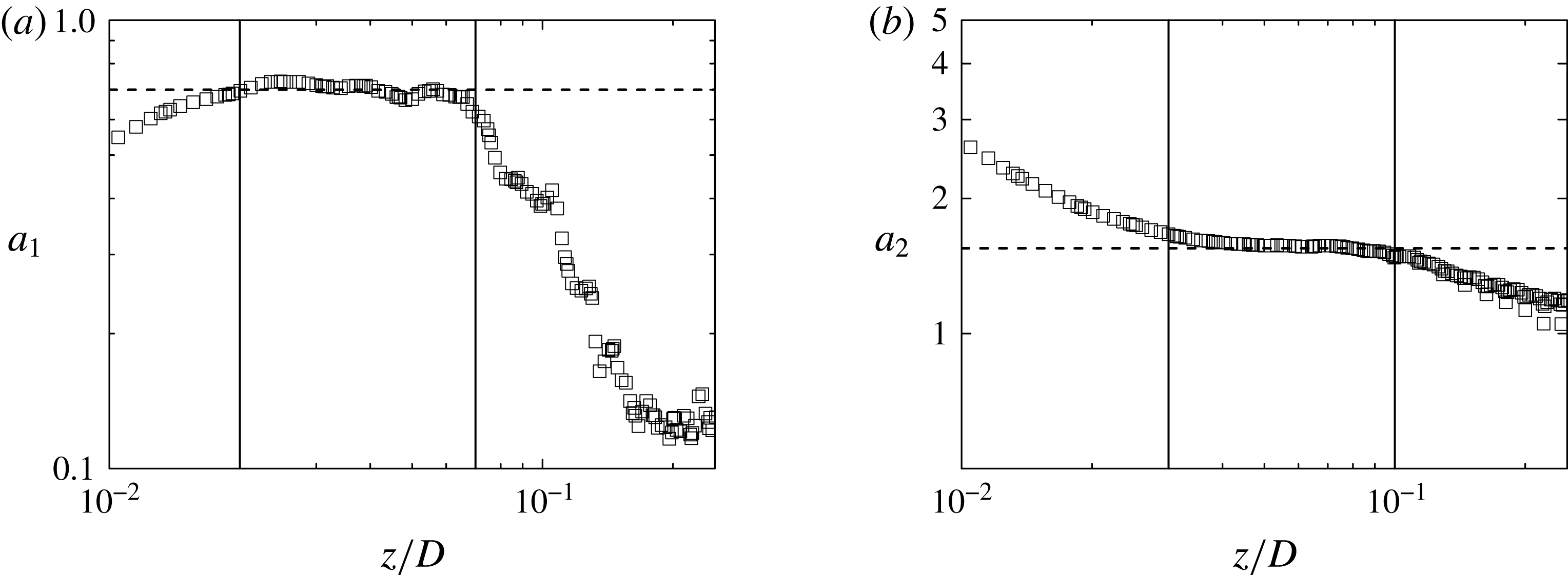
is a scaling constant of order unity. Figure 16(a) shows the calculated
 $a_{1}\equiv \unicode[STIX]{x1D705}_{f}/\sqrt{\unicode[STIX]{x1D6FC}g}z^{3/2}\unicode[STIX]{x1D702}^{1/4}$
as a function of
 $z/D$
using the DNS data. In the region
 $0.02\lesssim z/D\lesssim 0.07$
,
 $a_{1}$
remains approximately constant and does not change very much with
 $z/D$
. The dashed line shows the fitting result
 $a_{1}=0.7$
. Figure 16(a) thus confirms that (4.5) holds in the mixing zone.
(a) Calculated
 $a_{1}\equiv \unicode[STIX]{x1D705}_{f}/\sqrt{\unicode[STIX]{x1D6FC}g}z^{3/2}\unicode[STIX]{x1D702}^{1/4}$
as a function of
 $z/D$
in the thin disk. The two vertical lines indicate the region
 $0.02\lesssim z/D\lesssim 0.07$
, in which
 $a_{1}$
remains approximately constant, as shown by the dashed line with
 $a_{1}=0.7$
. (b) Calculated
 $a_{2}\equiv (\unicode[STIX]{x1D6FC}g)^{1/2}\unicode[STIX]{x1D702}^{1/4}\ell ^{2}/(2\unicode[STIX]{x1D705}z^{1/2})$
as a function of
 $z/D$
in the thin disk. The two vertical lines indicate the region
 $0.03\lesssim z/D\lesssim 0.1$
, in which
 $a_{2}$
remains approximately constant, as shown by the dashed line with
 $a_{2}=1.55$
. The calculations in (a) and (b) are conducted using the DNS data and are averaged across the cell thickness
 $L$
.

Using the same scaling arguments, we also find from (4.4) that
 $$\begin{eqnarray}\frac{u_{c}}{\ell _{c}}\simeq 2a_{2}\frac{\unicode[STIX]{x1D705}}{\ell ^{2}},\end{eqnarray}$$
where
 $a_{2}$
is another scaling constant of order unity. Equation (4.6) states that in the mixing zone the stirring frequency
 $u_{c}/l_{c}$
of the largest eddy is equal to the diffusion frequency
 $\unicode[STIX]{x1D705}/\ell ^{2}$
at
 $\ell$
(Tennekes & Lumley Reference Tennekes and Lumley1972). This suggests that turbulent mixing occurs in a spectrum of time scales from the largest eddy turnover time to the smallest Kolmogorov dissipation time. Figure 16(b) shows the calculated
 $a_{2}\equiv [(\unicode[STIX]{x1D6FC}g)^{1/2}/2\unicode[STIX]{x1D705}]\unicode[STIX]{x1D702}^{1/4}\ell ^{2}z^{-1/2}$
as a function of
 $z/D$
using the DNS data. In the region
 $0.03\lesssim z/D\lesssim 0.1$
,
 $a_{2}$
remains approximately constant and the dashed line shows the fitting result
 $a_{2}=1.55$
. Figure 16(b) thus confirms that (4.6) holds in the mixing zone.
Substituting (4.5) and (4.6) into (4.4), we find
 $$\begin{eqnarray}\unicode[STIX]{x2202}_{z}(z^{3/2}\unicode[STIX]{x1D702}^{1/4}\unicode[STIX]{x2202}_{z}\unicode[STIX]{x1D702})=\frac{1}{a_{1}a_{2}}z^{-1/2}\unicode[STIX]{x1D702}^{5/4}.\end{eqnarray}$$
Equation (4.7) has a power-law solution
 $\unicode[STIX]{x1D702}/\unicode[STIX]{x1D702}_{0}\sim (z/D)^{\unicode[STIX]{x1D716}}$
with
 $$\begin{eqnarray}\unicode[STIX]{x1D716}=-\frac{1}{5}\left[1+\left(1+\frac{20}{a_{1}a_{2}}\right)^{1/2}\right].\end{eqnarray}$$
In the above, we took the negative solution, as the positive solution
 $\unicode[STIX]{x1D716}=[(1+20/a_{1}a_{2})^{1/2}-1]/5$
is not physical. The temperature variance is a decaying function of
 $z$
. Using (4.8) together with the calculated values of
 $a_{1}=0.7$
and
 $a_{2}=1.55$
, we obtain
 $\unicode[STIX]{x1D716}\simeq -1.08$
. Without the DNS data as shown in figure 16, we will not be able to obtain the exact values of
 $a_{1}$
and
 $a_{2}$
as given above. In this case, we may assume
 $a_{1}\simeq 1$
and
 $a_{2}\simeq 1$
(and hence
 $a_{1}a_{2}\simeq 1$
) and obtain an estimated value of
 $\unicode[STIX]{x1D716}=-(1+\sqrt{21})/5\simeq -1.1$
using (4.8). The predicted values of
 $\unicode[STIX]{x1D716}$
are in good agreement with the experimental results as shown in table 1. The above analysis thus provides a useful framework to describe the essential dynamics of temperature fluctuations in the mixing zone.
5 Summary
We have carried out a systematic study of the mean and variance temperature profiles in turbulent Rayleigh–Bénard convection in a thin disk cell and an upright cylinder of aspect ratio unity. The temperature measurements were conducted along the central axis of the cell with varying Rayleigh numbers in the range between
 $9\times 10^{8}$
and
 $1\times 10^{10}$
and at two fixed Prandtl numbers
 $Pr=4.4$
and
 $Pr=7.6$
. Direct numerical simulation was performed in the same thin disk at
 $Ra=5\times 10^{9}$
and
 $Pr=4.4$
. Two distinct regions are identified. In the boundary layer (BL) region where the distance
 $z/\unicode[STIX]{x1D6FF}$
to the bottom conducting plate normalized by the thermal BL thickness
 $\unicode[STIX]{x1D6FF}$
is smaller than a critical value
 $\unicode[STIX]{x1D709}_{c}$
, the normalized mean temperature profile
 $\unicode[STIX]{x1D703}(z)$
is found to have a scaling form
 $\unicode[STIX]{x1D703}(z/\unicode[STIX]{x1D6FF})$
in both convection cells, and its functional form agrees well with the 2-D BL equation proposed by Shishkina et al. (Reference Shishkina, Horn, Wagner and Ching2015). Similarly, the measured temperature variance profile
 $\unicode[STIX]{x1D702}(z)$
is also found to have a scaling form
 $\unicode[STIX]{x1D702}(z/\unicode[STIX]{x1D6FF})$
with varying values of
 $\unicode[STIX]{x1D6FF}$
, and its functional form is well described by the recently derived 2-D BL equation by Wang et al. (Reference Wang, He and Tong2016). This equation further predicts the relative contributions of the five budget terms in (3.1), which are in good agreement with the DNS results.
In the mixing zone outside the BL region (
 $z/\unicode[STIX]{x1D6FF}>\unicode[STIX]{x1D709}_{c}$
), the measured
 $\unicode[STIX]{x1D703}(z)$
remains approximately constant, whereas the measured
 $\unicode[STIX]{x1D702}(z)$
is found to scale with the cell height
 $H$
in both convection cells and follows a power law,
 $\unicode[STIX]{x1D702}(z)\sim (z/H)^{\unicode[STIX]{x1D716}}$
with the obtained values of the exponent
 $\unicode[STIX]{x1D716}$
being close to
 $-1$
. The DNS data reveal that in the mixing zone the turbulent convection term in (3.1) is balanced primarily by the thermal dissipation term, and the other three terms are negligibly small. Based on these experimental and numerical findings, we derive a new equation for
 $\unicode[STIX]{x1D702}(z)$
in the mixing zone. This equation has a power-law solution and the obtained power-law exponent
 $\unicode[STIX]{x1D716}$
is in good agreement with the experimental and DNS results. Our experimental observation is consistent with a recent experiment (Wei & Ahlers Reference Wei and Ahlers2016), which reported that the measured
 $\unicode[STIX]{x1D702}(z)$
has a power law dependence for a liquid with
 $Pr=12.3$
and becomes a logarithmic dependence for a gas with
 $Pr\simeq 0.8$
. It was suggested that this change in the functional form of
 $\unicode[STIX]{x1D702}(z)$
may result from the
 $Pr$
-dependence, namely, fluids with
 $Pr>1$
favour the power law and those with
 $Pr<1$
favour the log law.
Our work thus provides a common framework for understanding the effect of BL fluctuations on the scaling properties of the mean and variance temperature profiles in RBC. Such an understanding is also relevant to many practical applications in wall-bounded turbulent flows. A further interesting extension of this work would be a study in gases or gas mixtures even with Prandtl numbers lower than those of air. In such fluids some basic assumptions of the underlying theory will no longer be valid and the scaling behaviour of the temperature and its fluctuations are expected to change.
Acknowledgements
This work was supported in part by the Hong Kong Research Grants Council under Grant nos. C6004-14G (X.W. and P.T.), A-HKUST616/14-A (P.T.) and HKUST16302715 (X.W.). X.H. acknowledges support through the China Thousand Young Talents Program and Shenzhen Startup Funds no. CB11409001. W.X. and J.S. were partly supported by the Research Training Group ‘Lorentz Force Velocimetry and Lorentz Force Eddy Current Testing’, which is funded by the Deutsche Forschungsgemeinschaft under Grant no. GRK 1567.