

Communities are social groups formed through interpersonal interaction and occur in all human societies (Murdock Reference Murdock1949). They may be variously described as bands, neighborhoods, or villages. In middle-range societies, community-level changes in social organization and interaction result from continuously negotiated, dynamic relationships through time (Pauketat and Alt Reference Pauketat, Alt, Van Dyke and Alcock2003; Stone Reference Stone2016). Demonstrating singular interpersonal interactions that constitute these communities in the archaeological record is difficult (Joyce and Hendon Reference Joyce, Hendon, Canuto and Yaeger2000; Yaeger and Canuto Reference Yaeger, Canuto, Canuto and Yaeger2000; but see Peeples Reference Peeples2018), but repetitive behaviors and practices can generate a physical record of interactions between people in “complex environmental, social, and historical contexts” (Stone Reference Stone2016:58).
The potential for and frequency of interaction, however, are affected by the physiographic setting of a community and the spatial distance between residences (Rohn Reference Rohn1977; Varien and Potter Reference Varien and Potter2008; Yaeger and Canuto Reference Yaeger, Canuto, Canuto and Yaeger2000). This relationship between interaction potential and spatial distance means “it is reasonable to expect that . . . patterns of interaction, and thus social communities, will be broadly reflected in patterns of spatial distributions of residence” (Peterson and Drennan Reference Peterson and Drennan2005:6, Reference Peterson, Drennan and Smith2011). Resulting residence locations in the archaeological record are the “fundamental physicality of human agency” (Stone Reference Stone2016:61; see also Joyce and Hendon Reference Joyce, Hendon, Canuto and Yaeger2000; Pauketat and Alt Reference Pauketat and Alt2005) that represents repetitive decisions made by each household to participate in its immediate social community (Murdock Reference Murdock1949; Yaeger and Canuto Reference Yaeger, Canuto, Canuto and Yaeger2000). The communities formed through these repetitive processes make up social and analytical units through which we can define decision-making processes, identify patterns of household aggregation and dispersal, and infer changes in social organization through time.
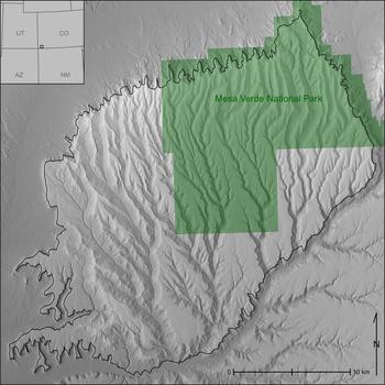
Here, we introduce a geospatial routine that provides a systematic empirical approach accounting for the dynamism of community constitution through time. This method enables us to identify groups of households and the distances members of those households might have traveled to construct and maintain a community. When applied through time, this method allows us to develop snapshots of change in community organization in any study area. To demonstrate the potential of this geospatial routine, we use a site database of all residences occupied between AD 600 and 1280 (Schwindt et al. Reference Schwindt, Kyle Bocinsky, Ortman, Glowacki, Varien and Kohler2016) on the Mesa Verde cuesta within Mesa Verde National Park in southwestern Colorado (Figure 1). We use a detailed analysis of occupation through time paired with spatial distributions to produce a cost-distance analysis that clusters contemporaneous households based on access to shared spaces for interaction.
The study area in Southwest Colorado. The Mesa Verde cuesta is outlined in black, and the extent of Mesa Verde National Park is shaded for reference.

We build on previous analyses using cost distances to categorize relationships between households and villages (also called “community centers”; e.g., Varien Reference Varien1999) by incorporating a computational means of determining the cost distance at which communities were likely maintained. Our method produces an emergent maximum cost-distance extent that households likely traveled to maintain local communities and is derived from a systematic assessment of changes in residential spatial organization through time. The results characterize dynamic social processes by calculating cost distances between households most likely to interact on a daily basis and reveal resilient structures in community spatial organization. We demonstrate that community size correlates in highly patterned ways with changes in regional population and the larger political landscape.
Habitation on the Mesa Verde Cuesta
The Mesa Verde cuesta, the physiographic feature that includes Mesa Verde National Park (Figure 1), consists of alternating mesas and canyons that range in elevation from 1,600 to 2,600 m. The geographic and environmental characteristics of the cuesta provided an ideal balance of growing season, precipitation, and soil quality (Benson Reference Benson2011; Schwindt et al. Reference Schwindt, Kyle Bocinsky, Ortman, Glowacki, Varien and Kohler2016; Varien Reference Varien, Varien and Wilshusen2002) that resulted in a productive maize growing niche in “more than 90% of years over the last two millennia” (Bocinsky and Kohler Reference Bocinsky and Kohler2014:4). Consequently, the Mesa Verde cuesta was occupied by ancestral Pueblo people between 6500 BC and AD 1300 (Lipe et al. Reference Lipe, Varien and Wilshusen1999) and was the most densely populated area in the northern San Juan region throughout the twelfth and thirteenth centuries (Glowacki Reference Glowacki2015).
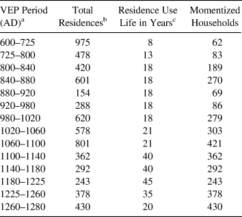
Our analysis uses “households” as the analytical unit to measure spatial patterning because decisions made at this scale are archaeologically represented by the placement of residential architecture. However, residential architecture in the Mesa Verde region changed through time, which directly affects how we implement our analysis. Basketmaker III (AD 500–700) households lived in subterranean pit structures, and household groups episodically aggregated throughout the period (Wilshusen Reference Wilshusen2018). Pueblo I (AD 700–890) households typically lived in clusters—known as “unit-type” pueblos (Lipe Reference Lipe, Lipe and Hegmon1989)—of small masonry structures with one large front room, two small storage rooms, and a subterranean pit structure to the south. Pueblo II (AD 890–1145) and Pueblo III (AD 1145–1280) residential architecture was built using increasingly shaped stone to construct uniform room blocks and masonry pit structures, both of which lasted longer than their earlier counterparts (Varien et al. Reference Varien, Ortman, Kohler, Glowacki and Johnson2007). The construction material used during each period directly correlates with the use life of residential structures through time. As the use of masonry increased, the use life of structures increased. For example, Basketmaker III architecture is estimated to have had a use life of eight years, whereas Pueblo III architecture was likely used for at least 45 years (Varien et al. Reference Varien, Ortman, Kohler, Glowacki and Johnson2007: Table 3). We account for the discrepancy between the length of time and use life by “momentizing” household population (Varien et al. Reference Varien, Ortman, Kohler, Glowacki and Johnson2007:280–282), a process explained below.
Community in the Mesa Verde Region
In middle-range societies, the interaction between households—“the minimal social units that form the building blocks for higher-order social groups” (Lightfoot Reference Lightfoot1994:12)—defines both residential and nonresidential relationships. Residential groups consist of kin-based relationships and act as intermediaries between the individual and the nonresidential community (Ware Reference Ware2014). Nonresidential groups “draw their members from multiple residential groups . . . [resulting in] a degree of community integration” (Ware Reference Ware2014:26) influenced through ritual structures by which “many basic social principles and divisions are constituted, transmitted, and reinforced” (Schachner Reference Schachner2001:168). A community of households, therefore, represents layers of residential and nonresidential groups that constitute interactive and exchange networks providing material and emotional support to people within the network (Milardo Reference Milardo1992).
In the U.S. Southwest, community is most often defined as “a group of people who lived in close enough proximity that individuals would (or could) come into face-to-face contact with each other on a regular, and possibly daily, basis” (Fast Reference Fast2012:17; see also Adler Reference Adler1990; Lipe and Hegmon Reference Lipe, Hegmon, Lipe and Hegmon1989; Mahoney et al. Reference Mahoney, Adler and Kendrick2000; Rohn Reference Rohn1977; Varien Reference Varien1999; Wills and Leonard Reference Wills and Leonard1994). A community created through repeated interaction among households is the smallest scale at which we can identify interresidential relationships in the archaeological record. Changes in these relationships through time can help us understand how a population responded to internal social and external environmental changes, reveal underlying organizational structures, and identify the consequences of disrupting those organizational structures. When embedded in larger polities, communities are presumably an essential intermediate level of interaction between the household and the polity.
Previous studies have quantified the proximity at which households likely interacted with one another on a regular basis by examining settlement patterns using least-cost analysis algorithms (e.g., Varien Reference Varien1999). Least-cost analysis is based on the principle of least effort, which assumes individuals use all available knowledge of an area or task to economize the behavior taken for a given action (Zipf Reference Zipf1949). When this principle is applied to distributions of archaeological residences, a “cost” of interaction between households can be calculated by determining difficulty of movement using Tobler's hiking function (Tobler Reference Tobler1993) on a digital elevation model (e.g., Herzog Reference Herzog, Bevan and Lake2013; Kantner Reference Kantner, Goodchild and Janelle2004; Surface-Evans and White Reference Surface-Evans, White, White and Surface-Evans2012). Tobler's hiking function calculates cost, measured in time of travel between two points at a walking velocity dependent on variation in elevation across a landscape. Variation in elevation causes a least-cost path to deviate from a straight line to find the path of least resistance (Surface-Evans and White Reference Surface-Evans, White, White and Surface-Evans2012). Results of this analysis are given in “cost kilometers” (cost km), which represent the equivalent distance an individual can travel on an established, level walking path given an identical amount of travel time.
Varien (Reference Varien1999) examined the spatial relationship of contemporaneous large, aggregated community centers and defined three cost km catchments: (1) a 2 cost km radius to capture “intensive cultivation and regular interaction among community members” (155), (2) a 7 cost km radius used to procure wild food and nonfood resources, and (3) an 18 cost km radius identifying the maximum extent of regular round trip travel by a household to a community center for religious and economic activity. Recent literature has primarily focused on the 2 cost km extent to assess social relationships in the upland U.S. Southwest (Bernardini and Peeples Reference Bernardini and Peeples2015; Coffey Reference Coffey2010; Crabtree Reference Crabtree2015; Hill et al. Reference Hill, Peeples, Huntley and Jane Carmack2015; Lipe and Ortman Reference Lipe and Ortman2000; Mahoney et al. Reference Mahoney, Adler and Kendrick2000; Murrell and Unruh Reference Murrell and Unruh2016; Varien and Potter Reference Varien and Potter2008). This catchment size is useful for understanding potential social relationships that existed between clusters of households, but the measurement is a necessarily static number representing what was inevitably a dynamic process (Schachner Reference Schachner2015). The spatial proximity of households within a social community would have continuously changed through time and fluctuated across space with varying topographies and sociopolitical pressures.
The Village Ecodynamics Project (VEP)—a multiyear, multi-institution project funded by the National Science Foundation (Kohler and Varien Reference Kohler and Varien2012; Kohler et al. Reference Kohler, Varien and Wright2010)—developed a Bayesian analysis to produce a demographic reconstruction that included the Mesa Verde cuesta from AD 600 to 1280 (Ortman et al. Reference Ortman, Varien and Gripp2007; Schwindt et al. Reference Schwindt, Kyle Bocinsky, Ortman, Glowacki, Varien and Kohler2016; Varien et al. Reference Varien, Ortman, Kohler, Glowacki and Johnson2007). The Bayesian analysis uses tree-ring dates from excavated sites, where they can be paired with detailed ceramic and architectural data, to estimate periods of residential site occupation for surveyed sites with surface ceramics and architectural features (Ortman et al. Reference Ortman, Varien and Gripp2007). The strong temporal correlation among changes in ceramic wares, design motifs, and residential architecture makes the Bayesian analysis an effective means of assigning occupation periods to all residences across a study area. The power of the Bayesian method is that it allows for a systematic assignment of occupation periods for residential sites across the cuesta using standardized lines of evidence; however, as is true with all archaeological analyses, some judiciousness in interpretation is required. Using the proportion of identified ceramic wares and other field observations, the VEP has estimated the probability each known archaeological residence was occupied within every period for six strata within the VEP II north study area (Schwindt et al. Reference Schwindt, Kyle Bocinsky, Ortman, Glowacki, Varien and Kohler2016), including Mesa Verde National Park. The data used here are a spatial subset of the Mesa Verde National Park stratum to include only residential sites located on the Mesa Verde cuesta (Figure 1). Table 1 summarizes the VEP periods and total number of known residences on the cuesta most likely occupied at some point during the associated period. The total number of residences, each representing one household, are “momentized” by dividing the average use life of residential architecture by the total length of each VEP period and then multiplying that proportion with the total number of residences assigned to the corresponding period (see Varien et al. Reference Varien, Ortman, Kohler, Glowacki and Johnson2007:282 for more detail). The resulting numbers of momentized households are used in the following analysis (Table 1).
Momentized Household Population on the Mesa Verde Cuesta by Period.

aOrtman et al. Reference Ortman, Varien and Gripp2007:250.
cVarien et al. Reference Varien, Ortman, Kohler, Glowacki and Johnson2007:282.
Calculating Communities
Although the elevation and aspect of the cuesta were advantageous for maize production, its topography limited areas suitable for agriculture and settlement and affected ease of travel. As Rohn (Reference Rohn1977:1) noted following a multiyear survey in Mesa Verde National Park, “The canyons do not prevent travel across them [but] several times as much time and energy is required to cross a canyon than to cover an equal distance on the mesa top.” The topography of the Mesa Verde cuesta clearly requires an approach to identifying communities that accounts for landscape influence on settlement patterns, subsistence, and interaction. To do this, we make three assumptions: (1) architectural remains reflect household agency (Stone Reference Stone2016), (2) intent to interact is reflected in residential location (Canuto and Yaeger Reference Canuto and Yaeger2000; Peterson and Drennan Reference Peterson and Drennan2005, Reference Peterson, Drennan and Smith2011), and (3) nearby households are more likely to interact on a daily basis than more distant ones (Varien Reference Varien1999).
To infer communities based on household proximity, we use all known residences on the Mesa Verde cuesta that had at least one occupied residence in any of the VEP periods from AD 600 to 1280 with a posterior probability equal to 1 as compiled by Schwindt and colleagues (Reference Schwindt, Kyle Bocinsky, Ortman, Glowacki, Varien and Kohler2016). For sites with multiple households, each household is considered, but all residences within a site share the location information. Although specific location information for each residence within a multi-household site would be ideal, such specificity is not necessary given the spatial scope of this project. Ultimately, households within the same site cluster within the same community at the end of the cost-distance and cluster analyses described below, just as would be expected if unique sets of coordinates for each household within the site were used.
For each period before AD 1100, a set of momentized households were randomly selected from all residences likely occupied during a given period (Table 1). In these cases, the cost-distance and cluster analyses described below were repeated five times on different momentized samples, and the arithmetic mean of these iterations is presented to best capture residential spatial patterns within each period. Although selecting a random subset of households for each iteration may not accurately reflect the actual residences occupied at any given time, it is an unbiased selection. The same analyses were applied to post–AD 1100 periods, but in these cases, each analysis was run only once because all residences are assumed to have been occupied for the entire length of each period. This method for determining changes in household interaction and organization through time removes researcher bias and subjectivity since it depends entirely on results from calculated cost-distance and cluster analyses. The methods described in the following sections are applicable to any study area with complete or nearly complete survey coverage.
Null Model Cost Distance
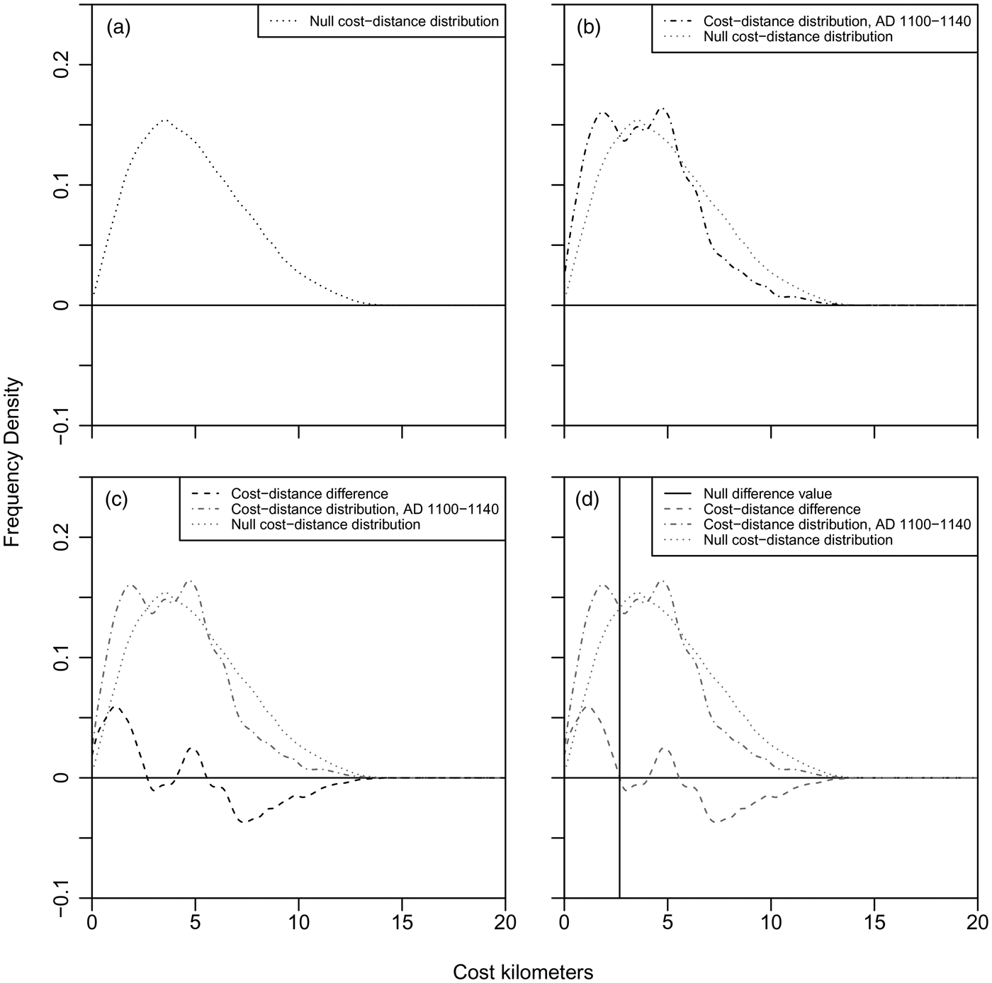
The elevation variability on the Mesa Verde cuesta drastically influences the cost distance of travel between households and, therefore, our ability to identify changes in aggregation and dispersal over time. To address this concern, a null model of household spatial distribution was calculated by randomly sampling 1,000 geographic coordinates from within the same extent of the cuesta for which we have empirical household location information. The cost-distance values between all pairs of coordinates in the null model are calculated and represent the expected distribution of interhousehold cost-distances if the landscape were randomly settled (Figure 2a). The same null model distribution was used for all periods because differences in the results of repeated sampling and cost-distance calculations were negligible.
(a) Null cost-distance distribution; (b) household cost-distance distribution for the AD 1100–1140 period; (c) difference between the null cost-distance distribution and household distribution; (d) the null difference value for AD 1100–1140. Each plot shows the frequency density, rather than a numerical count, along the y-axis of cost-distance distributions at each cost km along the x-axis.

Cost-Distance Comparison
Next, for each period, the cost-distance values between all pairs of contemporaneous households are calculated to determine the actual distribution of interhousehold cost distances, including any exaggeration as a byproduct of the landscape (Figure 2b). The null distribution of random interhousehold distances is then subtracted from the empirical cost-distance distribution for each period, as illustrated in Figure 2c for the AD 1100–1140 period. This difference (Figure 2c) represents the cost-distance distribution, freed from any topographic costs, of households in each period. We refer to the point at which households move from more aggregated (positive difference) to less aggregated (negative difference) than expected—when the difference between the null model and the empirical distribution equals zero (marked by the vertical line in Figure 2d)—as the “null difference.” Cost distances shorter than the null difference represent the distances at which households in each period are more aggregated than if the area were randomly settled. Since this process removes the topographic effects, we assume social factors can explain these proximities. Therefore, the null difference value is used to help create the similarity matrix for each corresponding period that ultimately informs the cluster analysis.
Null Difference Cost Distance
The overarching goal of this analysis is to calculate an emergent extent of potential regular household interaction, controlling for the topographic variability across a given landscape. Interaction between households, however, is not limited to occurring only at residential locations and can occur in any shared space. Therefore, households are clustered into potential communities based on similarity of travel costs to landscape cells across the cuesta. The following points summarize our study:
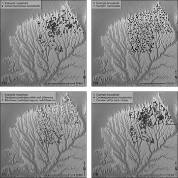
• The corresponding set of momentized households appropriate to each period (Table 1) is randomly selected from the total number of households for that period. For post-AD 1100 periods, all households in the corresponding period are selected because expected residence use life is greater than or equal to the period length (Figure 3a).
• A random sample of 1,000 coordinates is selected from the spatial extent of Mesa Verde National Park on the Mesa Verde cuesta (Figure 3b).
• The cost distance is calculated from each household to each randomly sampled landscape cells. The cost distances are recorded in a matrix where each column represents a household and each row, a sampled landscape cell.
• The cost-distance results are then converted to a presence value, 1, if the cost of travel from the corresponding residence to a landscape cell is less than the null difference for that period or to an absence value, 0, if the cost is greater than the null difference. Figure 3c illustrates this process as if it were taking place for a single site location, marked in white. This process is then repeated for all other contemporaneous households to the same set of randomly sampled landscape cells, which creates the similarity matrix used to group households in the following cluster analysis.
(a) All households occupied from AD 1100–1140 (the size of points are proportional to number of households at each site); (b) the locations of 1,000 random coordinates within Mesa Verde National Park on the Mesa Verde cuesta; (c) for a single example location, shown in white, all landscape cells within the null difference cost distance for this period are assigned a one (1), whereas cells outside this range are assigned a zero (0). This process is repeated for all contemporaneous sites before the cluster analysis is run, creating a similarity matrix where each row represents every sampled landscape cell within and beyond the null difference for a particular site, and each column represents every momentized household used in that particular cluster iteration; (d) results of the cluster analysis, which groups households based on the similarity in cost distances to landscape cells. (All maps of the clusters calculated for each period are available online as Supplemental Figures 1–50.)

Cluster Analysis
We use affinity propagation cluster analysis (Bodenhofer et al. Reference Bodenhofer, Kothmeier and Hochreiter2011; Frey and Dueck Reference Frey and Dueck2007, Reference Frey and Dueck2008) to group households into potential communities. This algorithm determines the optimal number of clusters for a dataset through an iterative process that creates the minimum possible sum of squared errors (Kintigh and Ammerman Reference Kintigh and Ammerman1982). Ultimately, each household is assigned the cluster to which it most likely belongs based on similarities in cost-distance proximity to landscape cells with other households within the same cluster. It is also possible for a household to be isolated if doing so minimizes the sum of squared errors (an example can be seen in Supplemental Figure 3). This approach removes the need for the researcher to predetermine the desired number of clusters, removing researcher bias and enhancing reproducibility. The resulting clusters from the analysis are our candidate communities (Figure 3d; maps for all periods are available online as Supplemental Figures 1–50).
Results: Characterizing Communities
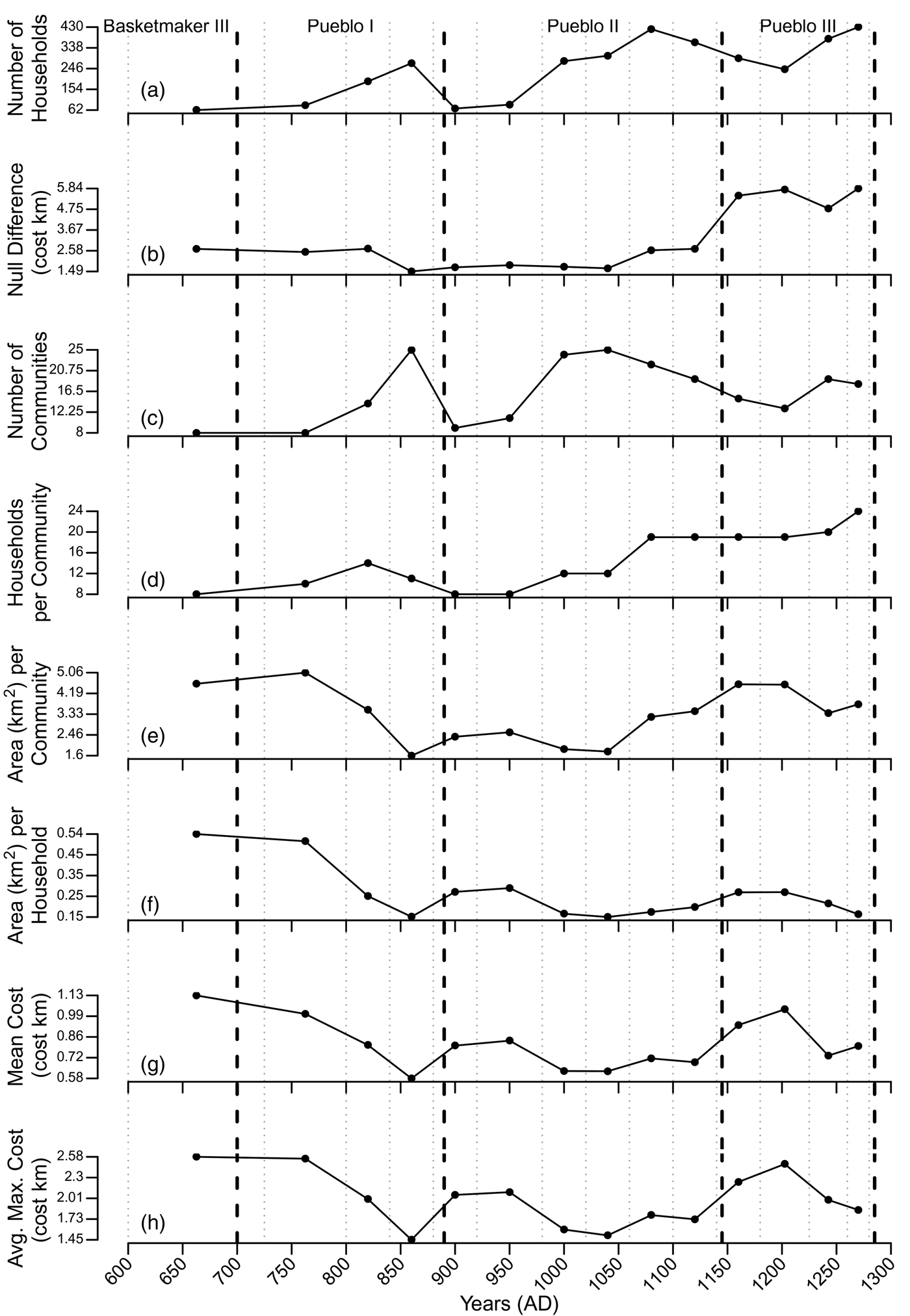
The communities produced by the cluster analysis were characterized along several dimensions to identify changes in social organization and responses to environmental variability through time (Figure 4). The averages for each metric are used throughout the results, although medians were also calculated and are available in Supplemental Table 1. Each metric used in Figure 4 is discussed briefly below.
• Number of households: the total momentized number of households (Table 1) likely occupied at any time in each period on the cuesta. Conventionally, archaeologists assume that each household represents 5–7 people (e.g., Lightfoot Reference Lightfoot1994), which likely represents the maximum for any household in its development cycle, given that simulation suggests an average momentary household size of approximately 3.3 people (Kohler Reference Kohler, Kohler and Varien2012). Figure 4a shows three cycles of population expansion and contraction on the Mesa Verde cuesta. Major episodes of population decline on the Mesa Verde cuesta began with periods of maize niche constriction (Bocinsky and Kohler Reference Bocinsky and Kohler2014) and decreased building activity (Bocinsky et al. Reference Bocinsky, Rush, Kintigh and Kohler2016).
• Null difference: the cost-distance spatial extent used in the cluster analysis (Figure 4b). The null difference provides a general idea of household aggregation and dispersal for each period at the landscape scale. A larger null difference means households were generally more aggregated at closer cost distances across the landscape than expected by the null model.
• Number of communities: the optimal number of communities determined by the cluster analysis, given similarities in the cost-distance spatial proximity of contemporaneous households to a random sample of landscape cells under the influence of the null difference for each period (Figure 4c).
• Households per community: the average number of households assigned to each community in each period (Figure 4d).
• Area per community: the average area in square kilometers within the “convex hull” enclosing all households in each community (Figure 4e). The convex hull is the minimum area required to encompass all points in a spatial dataset or, in this case, all households within a community (Jarvis Reference Jarvis1973; see example in Figure 3d).
• Area per household: the average area, in square kilometers, of land in the community convex hull divided by the number of households in that community (Figure 4f).
• Mean cost distance: the average cost distance between all pairs of households within each community (Figure 4g). For reference, 1 cost km represents approximately 12 minutes of travel time.
• Average maximum cost distance: the average maximum cost distance between households in each community (Figure 4h); the smaller the average maximum cost distance, the more compact the community.
The averages of metrics calculated from household clusters through time. Gray dotted lines mark boundaries of VEP periods. Black dashed lines mark Pecos period boundaries as derived by Bocinsky and colleagues (Reference Bocinsky, Rush, Kintigh and Kohler2016). The mean, median, and standard deviation for all periods are available online as Supplemental Table 1.

The results in Figure 4 show considerable variability in community organization and spatial relationships among households through time. Most importantly, the results indicate changes in structural elements, some of which reinforce our prior archaeological knowledge whereas others were unanticipated. Results from the first VEP period (AD 600–725; Basketmaker III) are shown in Figure 4 and reported in Table 2 but are not discussed because of the substantial disparity between the population of households and the comparatively small number of households after momentizing, which likely dramatically decreases the precision of our results for this period. We begin by discussing results most evident in period-to-period comparisons and conclude by examining results best perceived by looking at the entire temporal ensemble.

Pueblo I (AD 700–890)
The late Pueblo I period on the Mesa Verde cuesta was characterized by a large population with inter- and intracommunity aggregation previously noted across the central Mesa Verde (CMV) region (e.g., Wilshusen and Ortman Reference Wilshusen, Ortman, Wilshusen, Schachner and Allison2012). This aggregation is indicated by a simultaneous increase in the number of households and communities and a decrease in the mean and average maximum cost distance between households within the same community. As the Pueblo I period ended, the number of households and communities on the Mesa Verde cuesta declined as the maize dry farming niche contracted and annual growing conditions became increasingly variable (Schwindt et al. Reference Schwindt, Kyle Bocinsky, Ortman, Glowacki, Varien and Kohler2016). This decrease in the number of households and communities also corresponds with a decrease in tree-ring cutting date frequency, a proxy for building activity, throughout the upland U.S. Southwest (Bocinsky et al. Reference Bocinsky, Rush, Kintigh and Kohler2016). The remaining households on the cuesta during the transition between the Pueblo I and Pueblo II periods (AD 880–920) were living in more dispersed communities characterized by an increase to mean cost distance, area per community, and area per household.
Pueblo II (AD 890–1145)
As the population began to increase during the first half of the AD 1000s, the number of communities increased dramatically (Figure 4c), as did their degree of aggregation at the household (Figures 4 g and 4h) and community levels (Figure 4e). Simultaneously, an increase in the number of communities resulted in a number of households per community similar to that in Pueblo I, suggesting a return to organizational structures that were previously employed with a comparable household population.
As the number of households continued to increase in the late AD 1000s, the number of communities decreased, but remaining communities grew as the households per community and area per community increased. Communities were large; nonetheless, households continued to settle at relatively consistent cost distances that facilitated regular interaction with other households within each community (Figure 4g). These results suggest that households in the late AD 1000s were strongly influenced by the need to be close to existing residential clusters instead of settling in distant or open areas on the cuesta. This trend toward aggregation also reflects the characterization of the late Pueblo II period as the Chaco Phase of community-center construction in the Mesa Verde region, with intensive development of public architecture in highly aggregated communities (Glowacki and Ortman Reference Glowacki, Ortman, Kohler and Varien2012:Table 14.2). Communities also became increasingly standardized on the cuesta from AD 1060 to 1140 as households per community, area per household, and cost of interaction were mostly constant.
Pueblo III (AD 1145–1285)
Trends from late Pueblo II continued into early Pueblo III communities, but major changes began to appear in the early to mid-1200s. Communities became highly aggregated as the total cuesta population increased to its all-time maximum, resulting in a sharp decrease in the average maximum cost of interaction. Between AD 1240 and 1280, however, the mean cost of interaction increased even though more households were occupying smaller spaces. This discrepancy between aggregation and cost of interaction could be the result of some households moving into alcove settings. Households would have been increasingly aggregated within an area, but the cost of interaction between households would be disproportionately greater because of the cost to travel to and from alcove settings. Furthermore, the eastern portion of the cuesta was depopulating as households generally moved into steeper, alcove-containing canyons and mesas more centrally situated on the cuesta (Glowacki Reference Glowacki2015, Reference Glowacki, Lamoureux-St-Hilaire and Macrae2019), which also may have contributed to the increase in intracommunity cost distances. The 1200s were also the only time when a significant population increase coincided with a decrease in community area and, consequently, in area per household between AD 1260 and 1280 (Figure 4f). This fundamental organizational shift markedly changed the social landscape and may have destabilized social interaction, as the cuesta was completely depopulated by the end of the thirteenth century. Communities never returned to earlier, more dispersed organizational patterns but rather continued aggregating as the population on the cuesta continued to increase.
Macroscale Patterns
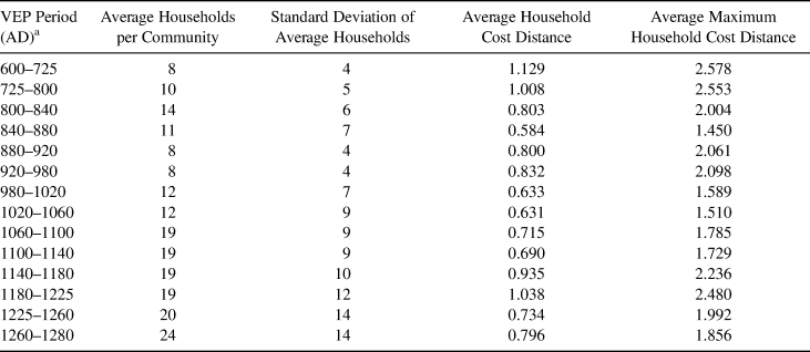
Cost-Distance Interaction. As noted earlier, the average maximum cost distance is the most comparable metric to the 2 cost km catchment used in previous studies. Our results generally support the use of a 2 cost km extent for the late Pueblo II and Pueblo III periods to examine household interaction (Table 2). In his analysis of intracommunity interaction from AD 1051 to 1290 in the CMV, Varien (Reference Varien1999) identified community catchments based on residential spatial patterning surrounding community centers, and he supported his results by comparing them to ethnographic examples of 2 km extents of interaction from around the world. Our results for the same interval average to 1.94 cost km (Table 2). The agreement between Varien's (Reference Varien1999) ethnographically supported measure and our results for the same period suggests the cluster analysis is accurately identifying overarching patterns of social interaction based on the placement of residential architecture. At the same time, our results improve on the established metric because they reflect the dynamic processes inherent in household relationships within the corresponding AD 1040–1280 period, extend the application of cost km community extents to the Basketmaker III through early Pueblo II periods (AD 600–1040), and are the emergent result of a computational process designed to remove researcher biases. We propose that our results can serve as updated community catchment sizes specifically tailored to periods in the CMV (Table 2). Researchers can also follow the protocol developed here to derive cost-distance estimates for regular interaction tailored to their specific areas of interest.
Structural Elements
An unexpected result is the relative stability of the area per household within communities after AD 900 (Figure 4f). The area per household is calculated by using a convex hull; however, our interpretations do not assume that households were limited to the imaginary boundaries created in the cluster analysis or that the land within these boundaries was wholly arable. However, a strong spatialized pattern was established by the mid-800s that continued throughout the rest of the study period: land per household in each community ranged from 0.15 to 0.27 km2. Studies on maize production and yield in the Mesa Verde region and broader U.S. Southwest (Benson Reference Benson2011; Bocinsky and Varien Reference Bocinsky and Varien2017; Ermigiotti et al. Reference Ermigiotti, Varien, Bohm and Kyle Bocinsky2018; Sherman Reference Sherman and Stuart2014) suggest that households must plant an average 0.14 km2 of land to reliably produce adequate amounts of maize to support their annual caloric needs.Footnote 1 Our results suggest intracommunity household spacing allowed households the necessary area to produce enough maize to sustain themselves for one to two years. Additionally, our research suggests it is likely that primary maize fields were located within the convex hull defining each community because an adequate area is maintained within the average community to satisfy the annual needs of each household through time. By the AD 1260–1280 period, however, there were more households on the cuesta than ever before living in communities that were organized differently than ever before, and the decrease in area per household to just 0.16 km2 suggests maize production from farms within the convex hull of the community was likely insufficient to meet the needs of all households within a community as a “major pan-regional drought” occurred in the late 1200s (Bocinsky and Kohler Reference Bocinsky and Kohler2014:2; Wright Reference Wright, Kohler, Varien and Wright2010).
Community Dynamics and the Environment
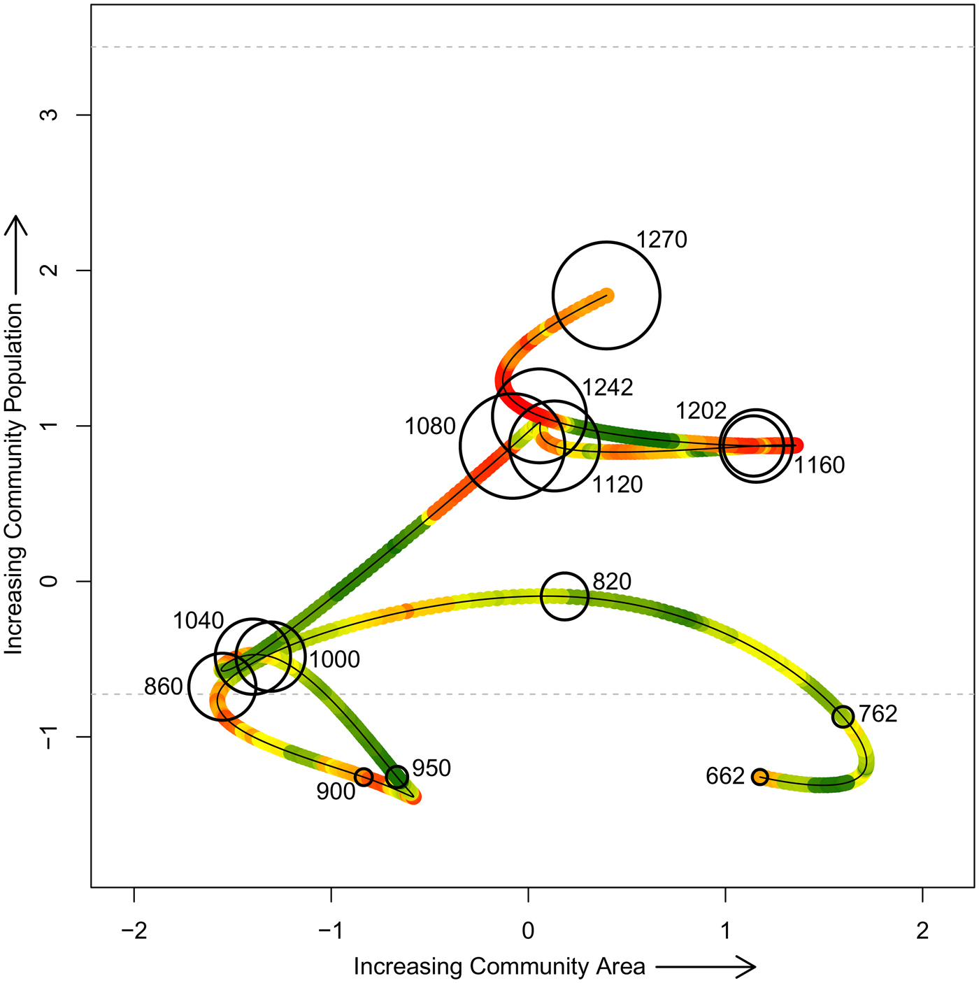
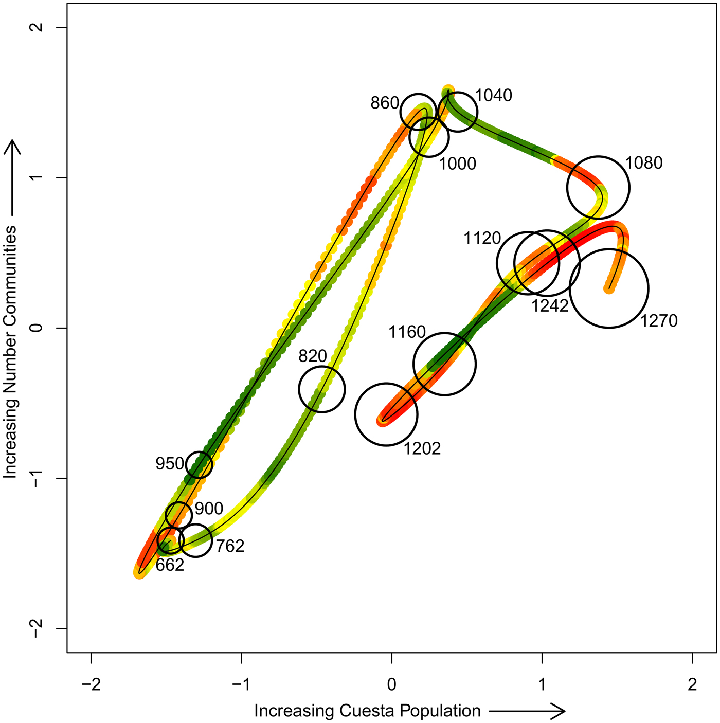
To better conceptualize the experience of households in communities on the cuesta, we examine the relationships between population, community size, and number of communities through time. Each variable in Figures 5 and 6, recast into z-score terms for each figure, has previously been defined except for the red-to-green color ramp. The color ramp represents the proportion of study area that falls within the maize growing niche, as calculated by Bocinsky and Kohler (Reference Bocinsky and Kohler2014), for each year from AD 600 to 1280. The maize growing niche is smoothed in Figures 5 and 6 using a lagged 20-year moving average to best reflect the remembered experience of people on the cuesta at any given time. The results are shown on a red (low productivity) to green (high productivity) spectrum.
The relationship between community area and population through time, shown in z-score terms across all periods. Each point is plotted at VEP period midpoints (AD), and the size of each point is proportional to the total momentized household population on the cuesta at that time. Community population is calculated as people per household times the number of households, using an estimate of 4.65 people per household (the mean of 3.3 [from simulation reported by Kohler Reference Kohler, Kohler and Varien2012] and 6 [a number commonly used in the Southwest, derived in part from Lightfoot Reference Lightfoot1994]). A 20-year smoothed maize productivity niche is shown on a red (low productivity) to green (high productivity) spectrum.

The relationship between number of communities and cuesta population through time shown in z-score terms across all periods. Each point is plotted at VEP period midpoints (AD), and the size of each point is proportional to average community population on the cuesta at that time. A 20-year smoothed maize productivity niche is shown on a red (low productivity) to green (high productivity) spectrum.

Figure 5 shows the relationship between average community area and average community population through time. The bubble size represents total momentized household population on the cuesta in each period (period midpoints are plotted in Figures 5 and 6). Figure 5 also displays, in horizontal dotted lines, a community population of 50 (lower) and 150 (upper) recast to the z-score metric of the y-axis. This plot reveals a changing relationship between community area and population through time that may be generally related to the Dunbar thresholds. The horizontal lines at 50 (lower) and 150 (upper) in Figure 5 are two of Dunbar's “magic numbers” (Dunbar Reference Dunbar1992). Dunbar considers the upper threshold to be the maximum number of individuals “with whom any one person can maintain stable relationships [which in turn] is a direct function of relative neocortical size” (Dunbar Reference Dunbar1993:691) and was found to be the mean size of bands and villages in modern hunter-gatherer groups (Dunbar Reference Dunbar1993: Table 1). In an analysis of settlement size and structure among contemporary New Guinea cultivators, Forge (Reference Forge, Ucko, Tringham and Dimbelby1972) also argued that 150 was a key threshold in community size beyond which basic relationships of kinship and affinity were insufficient to maintain social cohesion. Community sizes never exceeded 150 people even as the overall population on the cuesta continued to grow through time (Figures 4 and 5).
Figure 5 reveals two major organizational variants: one dominant from AD 600 to 1060 and the second from AD 1060 to 1260. A final organizational variant, from AD 1260 to 1280, is semidistinct. Transitions among low population periods from AD 600 to 1060 generally are pictured horizontally in Figure 5, which suggests community area and population were mostly independent in this early period. Household organization shifted from being highly dispersed with a very low population (AD 600–800) to being highly aggregated with a growing population (AD 840–1060). The AD 800–840 period is transitional between these organizational patterns, reflecting the aggregation that occurred in the study area as a result of emerging Pueblo I villages (Kohler and Reed Reference Kohler, Reed, Miller, Moore and Ryan2011).
Prior to AD 1060, communities did not grow proportionally in area as they increased in population. One possible reason for this trend is that farming before AD 1060 was more extensive than in later periods—farming that occurred not very near the residence and perhaps outside the community area—in addition to potential intensive farming near the residence. Kohler and Matthews (Reference Kohler and Matthews1988) suggested this farming strategy was also used during the Basketmaker III through Pueblo I periods in the nearby Dolores Archaeological Program study area. An extensive farming component may have been possible because of the generally productive maize growing niche during this early period on the Mesa Verde cuesta (there is variability but no extended periods of poor productivity) that would have prompted resource competition among neighboring communities. Alternatively, given the greater importance of wild foods and hunting for subsistence in this area during that time, we could infer that hunting and collection areas before AD 1060 were at least partially outside community boundaries, allowing community populations to grow or shrink without having much effect on community area.
Communities from AD 1060 to 1260 had a considerably larger population and were constrained to the middle range of variability in community area (Figure 5). The transition from the earlier AD 600–1060 organizational schema to the AD 1060–1260 period is diagonal, and we infer that community population could no longer expand without increasing the community area. It is also notable that the two main excursions into larger community areas were in the contexts of poor maize growing conditions. The dramatic shift between community organization from AD 600 to 1060 and AD 1060 to 1260 suggests a different sociopolitical environment among communities, and there likely were also different mechanisms for negotiating social and economic relationships within communities.
The AD 1260–1280 period is markedly different than any other during the occupation of the cuesta. Yet the organizational transition between the AD 1060–1260 period and the AD 1260–1280 period is reminiscent of the transition that occurred between the AD 600–1060 period and the AD 1060–1260 period. A significant population increase created another diagonal shift in Figure 5 that had not been explored by previous local societies. As in the previous shift, this suggests that a larger population in each community could not be accommodated without increasing the community area. The increase in both average community population and community area in the context of poor maize growing conditions suggests unprecedented, and likely stressful, social and economic conditions.
In Figure 6, we plot the number of communities against the total momentized household population on the cuesta through time, and the bubble size represents average community population. As we did in Figure 5, we interpret Figure 6 as showing two main variants of community organization with the final period being semidistinct from the second group. Prior to AD 1060, the number of communities and total cuesta population oscillated, and additional people on the cuesta were mainly accommodated by the formation of more communities. This pattern implies that the social and political organizations at the time could not accommodate larger community populations.
This circumstance changed soon thereafter, when cuesta population and community size made a correlated shift, but the simultaneous change in number of communities was negligible. Thereafter, community size remained large, and variability in cuesta population was once again accommodated by changing the number of communities. (The slope of the relationship between cuesta population and number of communities is similar to that in the earlier period, but the intercept is higher.) As in Figure 5, we infer that this change marks a shift in the sociopolitical environment from the AD 600–1060 period to the AD 1060–1280 period. In particular, it seems likely that the earlier societies did not share some aspects of organizational structures required to make these larger communities work. As seen in Figure 5, Figure 6 shows societies in the final period moving into a previously unexplored portion of the phase space, facing a likely uncomfortable combination of large community size, large cuesta population, and low maize production.
We suggest the organizational shift that occurred between the AD 600–1060 and the AD 1060–1280 periods signals a switch from communities as the largest social grouping to communities as an intermediate social level embedded within polities that included several communities. Our results follow, though they are slightly delayed relative to results from the simulation of polity formation in the VEP I study area—directly adjacent to but northwest of the cuesta—reported by Crabtree and colleagues (Reference Crabtree, Kyle Bocinsky, Hooper, Ryan and Kohler2017). From AD 600 to 980, the territory sizes of polities modeled by Crabtree and colleagues were log-normal in distribution, which is expected when territory size was not disproportionately advantageous for further growth. Following that, from AD 980 to 1260, simulated territory sizes were distributed according to a power law. This pattern is expected when the largest entities in the previous time step were the most likely to grow even larger, as in polity-formation processes when competition among social groups leads to the largest groups incorporating the smaller. These patterns are consistent with our findings, though we see this organizational shift occurring on the cuesta at AD 1060, not 980. This delay in sociopolitical reorganization is also evident in demographic and settlement changes as noted by Glowacki (Reference Glowacki2015, Reference Glowacki, Lamoureux-St-Hilaire and Macrae2019). It is interesting that even after this happened, as we can see from the results of this paper, communities remained a strongly identifiable element on the landscape. The resiliency of communities as a social unit of less than 150 people suggests this level of social organization was fundamental in these societies.
Discussion and Conclusions: Dynamic Communities
We have presented a geospatial analytic method that minimizes researcher biases when tracking changes in spatial organization and reveals underlying structural changes in communities through time that had not been previously identified. The results show the enduring importance of maintaining regular interaction among contemporaneous households and of the community in social organization even as the demographic, economic, and political contexts in which they are embedded were transformed.
Our method also reveals the average and maximum travel costs households likely invested through time to maintain relationships with neighboring households. The mean cost distance between households ranged from 0.58 to 1.13 cost km during the AD 600–1280 period (Table 2). In practice, these cost distances suggest that household members within the same community were traveling an average of 7–13 minutes to interact. The average maximum cost distance between households within the same community ranged from 1.45 to 2.58 cost km (Table 2), or 17–31 minutes of travel time, suggesting local and extended social networks could be maintained through regular interaction among neighboring households across the cuesta with relatively little time investment. However, we recognize household interaction and relationships were not limited to the clusters created in this analysis. The communities reconstructed here would have been nested in extended social networks (Milardo Reference Milardo1992) that reached beyond the local community, and at times, as argued above, these communities would likely have been nested in larger polities.
Maintaining proximity between households to sustain social communities coincided with the importance of access to subsistence resources for each household within a community. In our case, community spatial organization responded to an increasing population on the cuesta in the AD 1200s by including more households in smaller communities that had less area per household (Figure 4), even as production conditions remained very poor. Households were “packing” into communities (Schwindt et al. Reference Schwindt, Kyle Bocinsky, Ortman, Glowacki, Varien and Kohler2016), making it “very difficult, if not impossible, to implement an agricultural strategy” (Cordell et al. Reference Cordell, Van West, Dean and Muenchrath2007:386). The nearly vertical line connecting the 1240s with 1270 in Figure 5 shows that these communities were forced to accommodate more people without being able to appreciably expand their areas.
The decrease in both number of communities and cuesta population between 1160 and the early 1200s (Figure 6) may reflect the stress accompanying poor maize production and the (likely linked) breakdown of the Chaco regional system (Glowacki Reference Glowacki2015; Kohler et al. Reference Kohler, Ortman, Grundtisch, Fitzpatrick and Cole2014; Lipe Reference Lipe and Noble2004). Household population, however, increased on the cuesta throughout the 1200s (Figure 6). Elsewhere, Spielmann and colleagues (Reference Spielmann, Peeples, Glowacki and Dugmore2016) have noted increasing variation in village configuration and settlement sizes during this period. They consider this increased variation in settlement size—quantified here by an increase in standard deviation of average households per community (Table 2)—to be an early warning signal of social transformation (Spielmann et al. Reference Spielmann, Peeples, Glowacki and Dugmore2016), to which persistently poor growing conditions (Bocinsky and Kohler Reference Bocinsky and Kohler2014) and increasing violence in the late 1200s (Kohler et al. Reference Kohler, Ortman, Grundtisch, Fitzpatrick and Cole2014) contributed. Moreover, even as households were beginning to leave the CMV in the mid-1200s, people continued to arrive on the cuesta (Cameron Reference Cameron, Kohler, Varien and Wright2010; Glowacki Reference Glowacki2015; Schwindt et al. Reference Schwindt, Kyle Bocinsky, Ortman, Glowacki, Varien and Kohler2016). The Mesa Verde cuesta was the last best refuge—but still not good enough.
The results of this analysis show the dynamic but enduring nature of household relationships within communities. Residential spatial patterning that simultaneously facilitates face-to-face interaction between households but affords sufficient space for subsistence agriculture is integral to the creation and preservation of local communities in middle-range societies. Deleterious changes to this balance destabilize the underlying structures that simultaneously satisfy the social and agricultural needs of all households within a community.
The method presented in this article offers an approach to measuring changes in household relationships and community organization that does not require an assumption of community population, area, or total number of communities across a landscape. This method also provides a way to account for the dynamism of social relationships, increasing our ability to understand the experience of social actors in the archaeological record. By applying this geospatial protocol to other archaeological residential assemblages, we can explore the continuum of relationships between households within communities—and better understand the factors acting on and constraining these relationships—in diverse social, political, ritual, and environmental contexts.
Acknowledgments
This research was made possible with funding provided by the Coupled Natural and Human Systems program at the National Science Foundation (BCS-0816400), National Geographic (Grant #9100-12), University of Notre Dame Institute for Scholarship in the Liberal Arts, Washington State University, Notre Dame Presidential Fellowship in the Humanities and Social Sciences, and the John Templeton Foundation. Mesa Verde National Park, Crow Canyon Archaeological Center, Washington State University, University of Notre Dame, and the Santa Fe Institute provided institutional support. We would like to thank Scott G. Ortman and Dylan Schwindt for preparing and providing the data used in this project, Mark Varien and the rest of the VEP team, and Ian Kuijt, Mark Golitko, Rahul Oka, Kyle Bocinsky, Jean Larmon, and Sean Field for draft comments. We would also like to thank Di Hu for translating the abstract and the anonymous reviewers for providing constructive and helpful comments. Kohler is also affiliated with the Santa Fe Institute. The lead author would like to also thank Andrew I. Duff for serving on the WSU thesis committee that generated this research.
Data Availability Statement
Spatial data used in this project were reported in Schwindt and colleagues (Reference Schwindt, Kyle Bocinsky, Ortman, Glowacki, Varien and Kohler2016). Reproducible R code is available on GitHub at kmreese-io/Reese_et_al_2019.
Supplemental Materials
For supplementary material accompanying this paper, visit https://doi.org/10.1017/aaq.2019.74.
Supplemental Figures 1–50. Results of the cost-distance and cluster analyses for all time period iterations. The averaged metrics of these cluster communities are presented in Figures 4–6.
Supplemental Table 1. Mean (Avg.), Median (Med.), and Standard Deviation (SD) for All Metrics.