


1. IntroductionFootnote 1
The purpose of this paper is to provide new proposed estimates of Brazil’s per-capita GDP growth in the 19th century. Current statistical historiography of the period is based on successive editions of the Maddison Project Database (henceforth MPD), which gives continuity to Angus Maddison’s pathbreaking estimates of global economic growth since early Christianity (Maddison, Reference Maddison1995, Reference Maddison2001; among many others).
The latest editions of MPD for 2013, 2018, and 2020 suggest that Brazil stagnated in the 19th century, with per-capita GDP in 1900 only 0.8% higher than in 1800. The same source finds that Brazil’s per-capita GDP at the end of the Monarchy in 1890 was only 25% higher than on the eve of Brazil’s independence in 1820—with a growth rate of only 0.3% per year.
Economic historians sometimes simply reproduce such figures or argue that their analyses do not fundamentally diverge from the MPD’s. Thus, Abreu, Lago, and Villela (Abreu et al, Reference Abreu, Lago and Villela2022, p. 21) assert (in our translation) that “the periodisation today consensual is that Brazil’s per-capita income stagnated in the first half of the 19th century and increased only slightly in its second half”.
We believe this consensus to be based on inadequate methods, insufficient statistical evidence, and disregard for available historical evidence. After a review of the relevant literature, building on an empirical analysis by Tombolo (Reference Tombolo2013), summarized in Tombolo and Sampaio (Reference Tombolo and Sampaio2013), using new data sources and reasoned exploration of alternatives, we propose new estimates for real per-capita GDP growth in the 19th century.
Our best estimate is that Brazilians were twice as rich as they were in 1820 towards the end of the 19th century. Brazil’s output per capita trend growth rate is estimated to have been 0.9% per year from 1820 to 1900. Compared to the United States, this is an unimpressive performance, but on par with Western Europe and other Latin American countries during the same period. This performance, we submit, is more aligned with relevant facts of the country’s economic history in the period than the near-stagnation hypothesis embedded in the MPD.
The paper is organized as follows. In the next section, we review the sources of MPD for Brazil’s per-capita GDP in the 19th century. Section 3 provides new proposed estimates of Brazil’s per-capita GDP growth in that century. Section 4 explores relevant aspects of Brazil’s economic history, substantiating our preferred estimates. Section 5 converts our per-capita GDP estimates into 2011 USD dollars to compare with the MPD data from other countries and regions in the 19th century. We present our conclusions in Section 6. The Appendix contains details on data and statistical procedures.
2. MPD Brazil data reviewed
We first review the sources of MPD’s data on 19th century Brazil. Angus Maddison’s data on Brazil initially appeared in his 1995 book, Monitoring the World Economy, which includes numbers for per-capita GDP in constant dollars for 1820, 1870, and 1900 (Maddison, Reference Maddison1995: Table 1-3; sources in Appendix B, text: p. 93). For the 1850–1900 period, Maddison cited Goldsmith (Reference Goldsmith1986: pp. 22–23, 82–83) as the source, assuming that the growth rate in the 1820–1850 period was the same as that in the 1850–1913 period. His 1900–1985 GDP source was Maddison and Associates (Reference Maddison and Associates1992).
Maddison’s The World Economy: Historical Statistics (Maddison, Reference Maddison2003) contains Brazil’s GDP per capita data for 1820, 1850, and all years from 1870 onward (Table 4c, p. 142). Maddison Database Reference Maddison2010 reproduces the same series. However, as Barro and Ursúa (Barro and Ursúa, Reference Barro and Ursúa2008: App. A, Table A1) noted, Maddison’s numbers show an unexplained divergence from Goldsmith’s. While both authors report that per-capita GDP in 1900 is nearly the same as in 1850 (indicating zero growth in the second half of the century), Maddison supposes a linear trend from 1870 to 1890, a period for which Goldsmith’s numbers also show zero growth. Growth rates in the two series diverge similarly for the periods 1850–1870 and 1890–1900.
The first revision of Maddison’s data, in the context of the Maddison Project, was published in 2013.Footnote 2 Concerning Brazil’s data, the only meaningful change to the Maddison Database Reference Maddison2010 was the assumption of zero growth in per-capita GDP in the first half of the 19th century. The reference for this new assumption was Prados De La Escosura (Reference Prados De La Escosura2009: p. 301, Table 6), where “zero per capita for the early nineteenth century as suggested by Leff, Underdevelopment and Development, vol. 1, p. 33, was adopted.”
The revision in 2018 made more substantial changes: Maddison Project Database (MPD) (2018). Considering Barro and Ursúa’s observation about the unexplained divergence between Maddison’s and Goldsmith’s data, the original Goldsmith series for per-capita GDP was now adopted in full for the 1850–1900 period, expressed in constant dollars (Bolt et al, Reference Bolt, Inklaar, De Jong and Van Zanden2018). The hypothesis of zero growth in the 1800–1850 period was maintained. This series was repeated in the 2020 revision, now converted to constant dollars using a different methodology (Bolt and Van Zanden, Reference Bolt and Van Zanden2020).
We now examine MPD Brazil’s GDP per capita estimates separately for 1800–1850 and 1850–1900.
2.1. The 1800–1850 period
Prados De La Escosura (Reference Prados De La Escosura2009, Table 6, p. 301) explains that his figures for a stagnant Brazil in the 1800–1850 period were suggested by Leff (Reference Leff1982, p. 33).Footnote 3 Leff estimated the growth of nominal GDP based on the quantity theory of money and an ad hoc hypothesis on the velocity of money. To get numbers in real terms, he used a price index composed of three parts: (i) an index of prices of tradables based on a series of wholesale prices in Great Britain and the exchange rate mil-réis/sterling pound, assuming purchasing power parity; (ii) an index of food prices in Rio de Janeiro prepared by Lobo et al (Reference Lobo, Canavarros, Feres, Gonçalves and Madureira1971), assumed to indicate prices of the domestic agricultural sector in the country’s Southeast; and (iii) the trend in the price of a single commodity, manioc flour, extracted from a graph in an article by Mattoso (Reference Mattoso1978, p. 311), assumed to represent prices in the domestic agricultural sector in the country’s Northeast. The aggregate index is a weighted average of those numbers, with a weight of 0.45 for the index of tradables and 0.55 divided equally for the two regional indices.
Leff repeatedly stressed that the data and assumptions on which he based his estimates are precarious. He wrote about his output estimate: “Because of the rough nature of the data and assumptions which must be used, this procedure can at best yield tentative conclusions concerning the likely magnitudes of income growth” (Leff, p. 30). Before presenting the price index, he warned: “the very notion of ‘the’ rate of price inflation in Brazil as a whole during the nineteenth century raises conceptual problems which are serious and perhaps insurmountable” (Leff, p. 123).
Leff concluded that “income per capita seems to have risen at only a moderate pace in Brazil during the nineteenth century” (p. 33). His favored number is 0.1% per year.
Prados De La Escosura (Reference Prados De La Escosura2009) quoted this passage from Leff’s book to support his adoption of zero per-capita growth in Brazil’s first part of the 19th century—a hypothesis incorporated in the Maddison Project since 2013. However, a few pages later, Leff attempted a periodization of income growth in the 19th century and found that, considering five subperiods from 1822 to 1899, the growth of deflated currency stock was highest from 1822 to 1835 (p. 36). Leff commented on the result, asserting that “the rapid growth of the 1822–35 period is supported by the export figures for those years” (p. 37). In Leff, we may conclude that there is little basis for zero growth in Brazilian GDP per capita during the 1800–1850 period.
Abreu, Lago and Villela point out that the money stock series for the early 19th century were precarious. Instead, they base their presumption of a stagnated per-capita GDP in the first half of the century on the evolution of exports. However, a recent review of Brazil’s official export series in the 19th century (which most authors find unreliable at least through the early 1830s) presents a divergent view from stagnated per-capita exports in the first half of the century. Absell and Tena-Junguito (Reference Absell and Tena-Junguito2016) conducted an accuracy test on the official statistical values of Brazilian exports, finding evidence of considerable undervaluation of export prices. Once these were corrected, they concluded that Brazil’s export growth was more dynamic during the post-independence decades than in any other period in the 19th century. According to their online appendix, from 1821 to 1850, Brazil’s exports (in British pounds) grew 161.3% rather than the 62.5% shown in the official statistics used by Abreu, Lago, and Villela.
Leff’s “possible periodization” of real money stock growth and Absell and Tena-Junguito’s revision of Brazil’s export statistics lead to the conclusion that, based on these two variables, the first half of the 19th century was not one of stagnation. In Section 3, we present our proposed estimates of economic growth for the period, and in Section 4, we examine aspects of Brazil’s economic history that lend substance to these estimates.
2.2. The 1850–1900 period
We shift our attention to the second half of the 19th century, during which data were less scarce. Barro and Ursúa (Reference Barro and Ursúa2008)—who, since 2018, have been quoted by MPD as a new source for this period—affirm that their data for 1850–1900 were from Goldsmith (Reference Goldsmith1986). In the online appendix of their paper, they explain that they corrected Angus Maddison’s (Reference Maddison1995) estimates for 1850–1900, which he claimed were based on Goldsmith’s (Reference Goldsmith1986) data but diverged from this source. The implication is that the internationally accepted “bible” for the statistics on Brazil’s GDP growth in the second half of the 19th century is Goldsmith (Reference Goldsmith1986), to which we now turn.Footnote 4
Goldsmith started by constructing four yearly series, namely: exports plus imports of goods, urban wage income, central government spending, and money supply. He adopted an index-number format for each series and took a simple average to obtain a new series for 1850 to 1900 (and beyond), which he identified as the nominal GDP for the period.
Next, he calculated a simple average of four price indices (two of which were of questionable quality, as discussed in the Appendix), designating this average as the GDP deflator for the 1850–1900 period. The result of dividing the proxy for nominal GDP by the proxy for the GDP deflator yielded Goldsmith’s estimate of real GDP. Dividing real GDP by an estimate of the population, he obtained his real per-capita GDP proxy, which eventually found its way into the MPD and became the cornerstone for the presumption of a slowly moving Brazilian economy in the second half of the 19th century.
Far be it from us to depreciate Goldsmith’s pioneering effort to give order to the disparate economic series then available for the Brazilian economy. His strenuous efforts to put together, by himself and in a short period, nearly all available macroeconomic information on Brazil’s economy for the second half of the 19th century (and beyond) was nothing less than admirable. It is a pity that Harper & Row published only an editorially defective Portuguese-language version of his book, for an English version would have permitted a deeper historiographic critique of his approach.
With the benefit of hindsight and more recent empirical research, we submit, and further substantiate this assertion below, that Goldsmith’s figures on Brazil’s GDP cannot be accepted as a credible reflection of the country’s economic behavior in the second half of the 19th century. We believe these figures should be abandoned, yet replaced by what?
Tombolo (Reference Prados De La Escosura2013), summarized in Tombolo and Sampaio (Reference Tombolo and Sampaio2013), used the figures unearthed by Goldsmith and obtained a more acceptable proxy for the evolution of Brazil’s GDP per capita in the 19th century. He constructed yearly series for population, government revenues, money supply, goods imports, and goods exports for the 1820–1946 period.
These series are similar to Goldsmith’s, with population replacing urban wage income and government revenues replacing government spending. However, instead of taking a simple average of the series, as Goldsmith did, Tombolo first regressed them on Haddad’s (Reference Haddad1978) widely used series for nominal GDP in the 1900–1946 period. He then used the coefficients of this regression as weights to construct estimates of yearly nominal GDP from 1850 to 1900 by properly aggregating the series of population, government revenues, imports, exports, and money supply for this period.
To obtain a GDP price deflator, Tombolo first estimated a regression of five price indices on estimates of the GDP price deflators for 1889–1947.Footnote 5 He then used the estimated coefficients of this regression to generate a GDP price deflator for 1820–1900 as a composite of the five price indices. By dividing nominal GDP by the GDP price deflator, he obtained real GDP estimates, which, once divided by population, yielded a series of real per-capita GDP since 1820.
There are some problems with Tombolo’s estimates. For example, population is a poor choice of a regressor in an equation purporting to represent nominal and not real GDP. In addition, his choices of the regressors for the GDP price deflator are problematic. For example, he included as regressors both the exchange rate of the mil-réis to the British pound and the product of this exchange rate by the UK’s wholesale prices, which seems incongruous. Furthermore, his GDP price deflator may underestimate the course of inflation since the coefficients of his five price-index regressors add up to less than one.
Nonetheless, as acknowledged by Abreu, Lago, and Villela (Abreu et al, Reference Abreu, Lago and Villela2022, pp. 43–44), the figures produced by Tombolo are an improvement over Goldsmith’s estimates. They are the best guesses that we currently have on Brazil’s per-capita GDP for the 19th century.Footnote 6
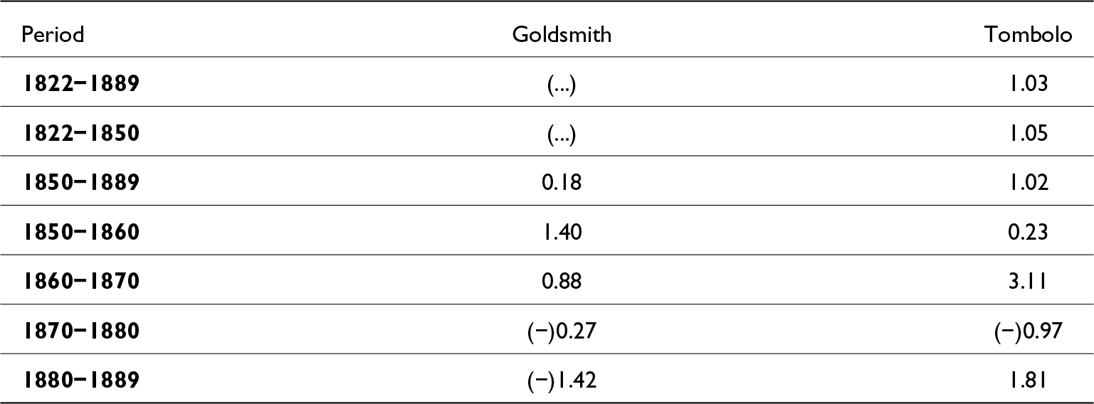
Table 1 compares the yearly GDP per capita growth rates estimated by Goldsmith and Tombolo for the Monarchy and relevant subperiods. We used Mortara (Reference Mortara1941) population estimates for both series to make them comparable on a per-capita basis. The figures for Goldsmith start in 1850. For 1850–1889, Goldsmith had 0.18% while Tombolo suggested— 1.02%—five times as large a value. For the Monarchy as whole, from 1822 to 1889, Tombolo estimated a yearly growth rate of 1.03%, with roughly equal trends for 1822–1850 and 1850–1889.
Goldsmith’s and Tombolo’s estimates of Brazil’s yearly real per-capita GDP growth in the monarchy, 1822–1889 (%)

Source: Estimated from Goldsmith (Reference Goldsmith1986, p. 22) and Tombolo (Reference Tombolo2013, p. 49) using population data from Mortara (Reference Mortara1941).
Goldsmith’s figures for 1850–1860 and 1870–1880 were somewhat higher than those of Tombolo; however, they were substantially lower for the periods 1860–1870 and 1880–1889. Goldsmith’s negative estimate for 1880–1889 is particularly awkward, for this was a decade in which railroads and European immigration were both growing at rapid rates accompanying the expansion of coffee production in São Paulo, the country’s Northeast was recovering from the devastating droughts of the late 1870s, and the Amazon rubber boom was gaining speed.
We conclude that Goldsmith (Reference Goldsmith1986) underestimated Brazil’s growth in the second half of the 19th century. In the next section, we develop new estimates of Brazil’s economic growth in the 19th century, building on Tombolo (Reference Tombolo2013).Footnote 7
3. Re-estimating Brazil’s GDP growth in the 19th century
In the following, we maintain the logic of Tombolo’s approach (Tombolo, Reference Tombolo2013) while attempting to address the problems in his empirical procedures. We start with nominal output per capita, followed by the estimation of price deflators, to conclude with new proposed estimates of Brazil’s real per-capita GDP in the 19th century. We begin the analysis in 1820, as data for the earlier part of the century are remarkably scant.
3.1. Estimating nominal output per capita
We aim to construct an index number representing nominal GDP from three macroeconomic variables at current prices: an arithmetic mean of goods exports and imports in national currency (which we denominate as “foreign trade index”), an arithmetic mean of central government’s revenues and expenditures (which we denominate as “government budget”), and a money supply series. All variables are expressed in per-capita terms. We chose these variables because of their direct association with nominal GDP and their availability for most of the 19th century. The Appendix details the data sources for these series.
Our first task is determining the weights with which these three variables enter the construction of nominal GDP. We obtain these weights with a regression of nominal GDP on the three variables in the 1900–1947 period. For this purpose, we use Haddad’s (Reference Haddad1978) nominal output estimates for 1900–1947. The results of this regression are in the Appendix. Applying the weights obtained in the regression to the values of the independent variables along the 19th century, we built a nominal output per capita series from 1820 to 1900, using a Laspeyres index based on 1900:
 \begin{equation*}\textit{Y}_\textit{t}^\textit{n} = 100 \times \left( {0.461783 \times {{\widehat {\textit{FT}}}_t} + 0.179754 \times {{\widehat {\textit{GB}}}_t} + 0.387892 \times {{\hat {\textit{M}}}_\textit{t}}} \right)\end{equation*}
where the hats on top of the variables indicate the (gross) percentage change between year  $t$ and year 1900;
 $Y_t^n$ is nominal GDP,
 $F{T_t}$ is a foreign trade index obtained by the arithmetic mean of exports and imports in domestic currency;
 $G{B_t}$ is a government budget index obtained by the arithmetic mean of government expenditures and revenues; and
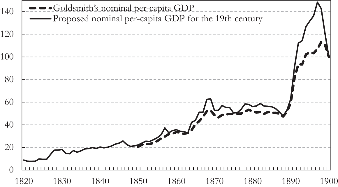
 ${M_t}$ refers to a money supply series. All variables are in per-capita terms.Footnote 8 Figure 1 compares our series of nominal per-capita output for 1820–1900 with Goldsmith’s for 1850–1900.
Figure 1 makes it clear that, except in the 1890s, the general tenor of our series is like that of Goldsmith’s, and even in this last decade, the cumulative growth rates of the two series are similar. We conclude that the exclusion of the payroll series and the introduction of government taxes do not change much our nominal GDP series from that obtained by Goldsmith over the 1850–1900 period. The main difference between our results and Goldsmith’s is the choice of deflators to obtain real output, as we explain in the following.
Probable level of brazilian nominal per-capita GDP in the 19th century (1900 = 100).

3.2. Estimating the output deflator
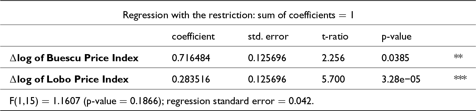
The next step is to select a deflator to obtain a real output series. In the Appendix, we provide a detailed explanation of the construction of the deflator. Briefly, the only methodologically sound price index for (part) of the period is the wholesale price index of Catão (Reference Catão1992). Unfortunately, it was only available from 1870. For the previous decades, the following best choices are the cost-of-living index of Lobo et al (Reference Lobo, Canavarros, Feres, Gonçalves and Madureira1971) and a general price index of Buescu (Reference Buescu1973). For the 1820–1870 period, we constructed a Laspeyres index from these two indices, based on 1870, with weights given by a regression of the Catão index on log first differences of these two series in the 1871–1887 period, as follows:
 \begin{equation*}{\textit{P}_\textit{t}} = 100 \times \left( {0.716484 \times {\hat {\textit{B}}_\textit{t}} + 0.283516 \times {{\hat {\textit{L}}}_\textit{t}}} \right)\end{equation*}
where the hats on top of the variables indicate the (gross) percentage change between year  $t$ and year 1870;
 ${\mathit{P}_t}$ is our proposed output deflator,
 ${\mathit{B}_t}$ is the Buescu price index and
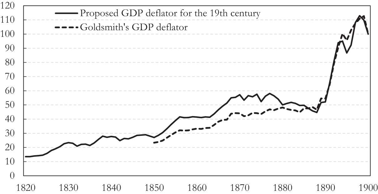
 ${\mathit{L}_t}$ the Lobo price index. This weighted average is then spliced into the Catão index in 1870, which is thus extended back to 1820. We use this index as a deflator of nominal per-capita GDP from 1820 to 1900. This index is in Figure 2, where we also display Goldsmith’s output deflator for 1850 to 1900.
Goldsmith’s and our proposed deflator (1900 = 100).

Goldsmith constructed his deflator as a simple average of four price indices: Buescu (Reference Buescu1973), Lobo et al (Reference Lobo, Canavarros, Feres, Gonçalves and Madureira1971), Onody (Reference Onody1960), and Vieira (Reference Vieira1947).Footnote 9 We did not include Onody’s or Vieira’s price indices in our equation because of their shortcomings, as explained in the Appendix. Furthermore, we used appropriately weighted Buescu’s and Lobo’s indices as proxies to Catão’s index.
From 1850 to 1879, Goldsmith’s and our indexes exhibit nearly the same yearly inflation rate (2.5% vs. 2.4%). From 1879 to 1887, our index shows a annual deflation of about 2.0%. Goldsmith’s index displays a yearly inflation rate of 0.3% in the same period. The index used by Goldsmith fails to capture the deflation, particularly evident in import prices in these years. From 1888 to 1900, the yearly inflation rate was 5.7% for the Goldsmith deflator and 6.2% for ours.
Having established a deflator, we proceeded to estimate Brazil’s real output per capita from 1820 to 1900, first comparing our results with those of Goldsmith for the 1850–1900 period.
3.3. Probable evolution of Brazil’s real per-capita GDP from 1850 to 1900
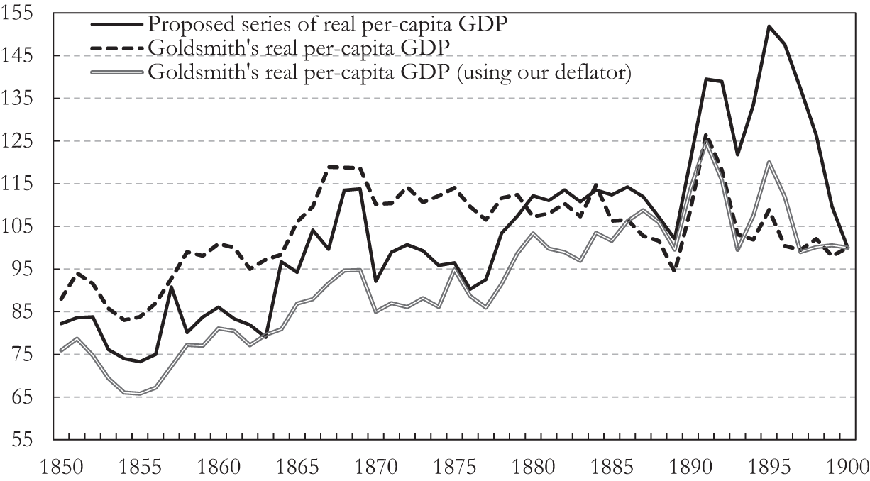
We obtain an estimate of Brazil’s real per-capita output from 1820 to 1900 by dividing per-capita nominal GDP by the deflator developed in the previous section. Figure 3 compares the evolution between 1850 and 1900 of our real per-capita output series (the continuous black line) with that of Goldsmith (the black dashed line). The figure also shows the behavior of Goldsmith’s nominal output estimates deflated by our price index (the grey line). All series are in index number form, with 100 in 1900.
Probable levels of Brazilian real per-capita GDP in the second half of the 19th century (1900 = 100).

Overall, our series displays a higher per-capita output growth rate, which is why most of the time it lies below Goldsmith’s series (all series are equal to 100 in 1900). The difference is primarily due to the deflators, since when our deflator adjusts Goldsmith’s nominal series, the growth pattern of his inflation-corrected series is similar to ours. Our series diverges from Goldsmith’s growth rates mainly between 1878 and 1887, when the inflation rates of the two deflators differ sharply. In this period, our series’ yearly growth rate of real per-capita output is 0.9%, whereas Goldsmith calculated a negative rate of −0.9%. In the last decade of the century, our series displays sharper fluctuations than Goldsmith’s, but both overall growth rates are similar.
Having argued that the differences between our results and those of Goldsmith for the second half of the century are primarily due to the price deflators, we proceed to a more detailed analysis of our series for the entire 1820–1900 period.
3.4. Per-capita GDP growth in the 19th century
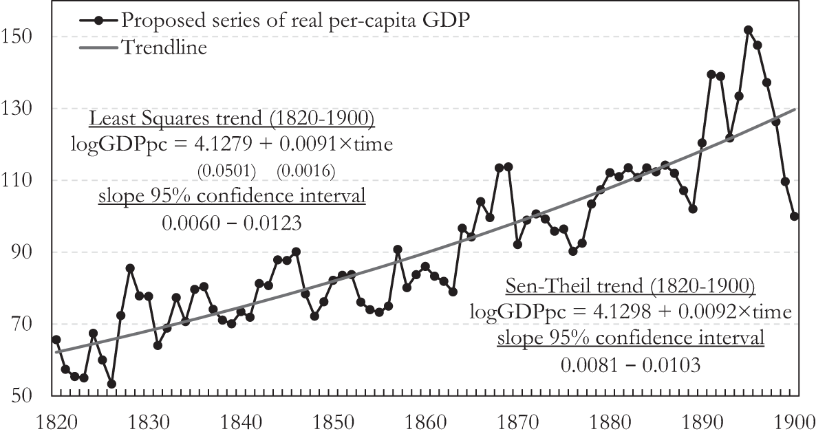
The black dotted line in Figure 4 displays the evolution of our estimated real per-capita output series from 1820 to 1900. Two features are apparent. First, the trend is clearly positive. Second, the series is highly volatile, with periods of expansion alternating with periods of contraction of varying magnitude and duration.
Our estimate of Brazil’s real per-capita GDP from 1820 to 1900 and its trendline.

Because of this high volatility, we decided to fit a log-linear trend to the series using both Least Squares and the Theil–Sen estimator. Unlike Least Squares, the latter is robust to outliers,Footnote 10 which are particularly evident in the last decade of the 19th century. In Figure 4, the black trend line of the Theil–Sen estimator has a slope indicating an annual growth rate of 0.9% between 1820 and 1900.Footnote 11
The point estimate of the slope by the two methods is the same, 0.9% per year, but the 95% confidence interval is bigger for Least Squares (0.60–1.23%) than for the Theil–Sen estimator (0.81–1.03%). If we accept the bigger interval for prudence, we have a range from 0.6% to 1.2% for the average annual growth of the Brazilian economy between 1820 and 1900.
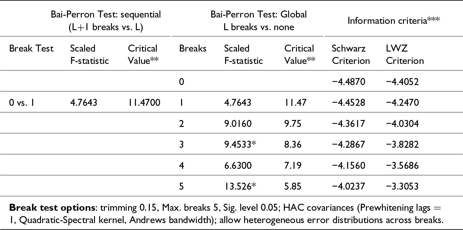
Searching for possible multiple breakpoints in the series, we applied Bai–Perron (Bai and Perron, Reference Bai and Perron2003) tests, as explained in the Appendix. None of these tests suggested the existence of breakpoints in the series, supporting the adoption of the same trend growth rate for the 1820–1900 period, meaning that Brazil’s per-capita output trend-growth was 0.9% per year with a range of 0.6–1.2%.Footnote 12
These results are in sharp contrast to previous studies on the behavior of Brazil’s economy in the 19th century. Leff (Reference Leff1982, pp. 33–34) claimed that “income growth in nineteenth-century Brazil probably did not exceed the country’s rate of population increase.” Furtado (Reference Furtado, Aguiar and Drysdale1963, Ch. 19) asserted that real per-capita income declined in the first half of the century, while Prados De La Escosura (Reference Prados De La Escosura2009, p. 301) assumed that the Brazilian economy stagnated in the same period. Also, our suggested range for the yearly trend growth rate of real output from 1820 to 1900 (0.6% to 1.2%) is well above the 0.2% to 0.5% range that Abreu, Lago, and Villela (Abreu et al, Reference Abreu, Lago and Villela2022, p. 65) hypothesized for the mean growth rate of real per-capita output during the Monarchy (1822–1889).
Given these differences, we should stress the tentative nature of our results. We used indirect methods to estimate output growth. We have no observations on production volumes, only the monetary series is deflated by price indices. The margin for measurement error is large, indeed.Footnote 13
One possible source of upward bias in our estimates is the inclusion of only market-related variables in the nominal GDP regression, as these variables may not capture the evolution of the slow-moving subsistence sector.Footnote 14 This criticism, incidentally, would also apply to all previous studies, which considered only market-related activities.
It is however our understanding that production of subsistence food for the predominant rural population had, by and large, very low activity levels; in the words of Furtado (Reference Furtado, Aguiar and Drysdale1963, pp. 130–131): “because it was based on cattle breeding and farming with the most rudimentary techniques, its economic density was reduced to a minimum”. On the other hand, the production level of the commercially oriented subsistence sector was related to that of the export sector. In the case of Bahia, for instance, Barickman (Reference Barickman1998, pp. 79–80) shows that the ups and downs of the price of cassava flour (a staple food in the region), sold by small farmers to sugar estates, and also to Salvador, the provincial capital, followed closely the export price of sugar (in other words, production of this sector would be taken care of by the export series that we used).
The presumption of the smallness of the subsistence sector is substantiated by the estimate of Brazil’s per capita income in 1872 by Bertola et al (Reference Bertola, Castelnovo and Willebald2012, p. 8). This paper estimates GDP per capita from the income side, utilizing information from the 1872 Census and other administrative records, and includes an imputation for the incomes of enslaved persons. It thus supposedly captures the income generated in the subsistence sector. Notwithstanding, the figure that the authors obtain for Brazil’s GDP per capita in 1872 is 118 mil-réis, practically the same as the 119 mil-réis estimated by Goldsmith (Reference Goldsmith1986, p. 23), who used a methodology similar to ours, that is, considering only market-related activities.
Given the weakness of the available data, our results can only be considered provisional. Our claim is the use of series similar to those of previous studies. The difference is that our monetary series are newer and aggregated according to a methodology that respects their relationships with nominal output in the 20th century. In addition, our price deflator series used the only truly reliable price index for the later part of the 19th century (Catão, Reference Catão1992) while estimating the inflation rate in the rest of the century with a combination of the two next-best indices (Lobo et al, Reference Lobo, Canavarros, Feres, Gonçalves and Madureira1971; Buescu, Reference Buescu1973), which is respectful of their relationships with the Catão index in the 1871–1897 period. In the Appendix, we provide a detailed discussion of the construction of our series and make it available for future researchers who may wish to test its robustness.Footnote 15
Our proposal is certainly not perfect, but after a reasoned exploration of alternatives, it appears to us to be the best option, based on our research. More importantly, our quantitative findings are backed up by historical and historiographic evidence, which we present in the following section.
4. Historical and historiographic evidence
This section reviews relevant historical and historiographic material on Brazil’s economy in the 19th century (Bethell, Reference Bethell1989)Footnote 16. First, we briefly address the second half of the century, as our findings for this period do not diverge substantially from those in the literature. We then proceed to a deeper analysis of the country’s economy in the first half of the 19th century, where our statistical findings diverge from the current historiographic consensus.
4.1. The second half of the 19th century
Furtado (Reference Furtado, Aguiar and Drysdale1963, Ch. 25) asserted that the second half of the 19th century had significant growth. Only Leff (Reference Leff1982) challenged this evaluation based on the disputable quantity theory of money and the use of inadequate price deflators. Goldsmith (Reference Goldsmith1986) arrived at a lower growth rate of output than ours for the period 1850–1900. However, as we hope to have convincingly shown, this is only because he uses inappropriate price deflators to generate the real output series.
Moreover, several studies document relevant growth sources in the second half of the century. The extraordinary expansion of coffee cultivation in São Paulo is described in Bacha (Reference Bacha, Martins and Johnston1992, pp. 18–28). The positive effect of this expansion on income and production diversification, especially when free labor became predominant in the coffee sector, has been emphasized since Furtado (Reference Furtado, Aguiar and Drysdale1963, Ch. 25, 26). The favorable impact of the railroad expansion from 1850 onward—essentially financed by British capital—is analysed in Summerhill (Reference Summerhill2003); also, Herranz-Loncán (Reference Herranz-Loncán2014). As noted by Franco (Reference Franco1991, Ch. 4), it is also worth mentioning that the country’s financial relationship with the rest of the world improved over the last two decades of the century, paving the way for better access to international finance.
After 1870, there are indications that mass immigration, stimulated by coffee expansion, significantly contributed to human capital (see Hall, Reference Hall1969; Holloway, Reference Holloway1974; Barros, Reference Barros2016). The number of immigrants arriving from 1871 to 1900 was 1.86 million, an impressive number compared to the total population of 10.1 million in the 1872 census (Merrick and Graham, Reference Merrick and Graham1979: p. 37). Over the course of those three decades, the proportion of foreign-born male workers in the labor force doubled, reaching 10% by 1900. In the São Paulo province, this proportion was 22% in agriculture and 47% in non-agricultural activities, with 57% in industry. The data for 1900 provide a strong indication of the educational superiority of the foreign-born, as their literacy rate was 43%, compared to 23% for the native-born. The proportion of the foreign-born with primary education was twice as high as that of the native-born; a proportion close to three times as high, in the case of secondary or college education (Merrick and Graham, pp. 105–111).
The 1870s also witnessed the beginnings of an industrialization drive, especially in cotton textiles. Tariff protection for this sector increased in the following decades, favoured by the growing influence of pro-industry interests and by investments from the importing business (Versiani, Reference Versiani1979, Reference Versiani, Bielschowsky, Boianovsky and Coutinho2023; Dean, Reference Dean1969: Part One).
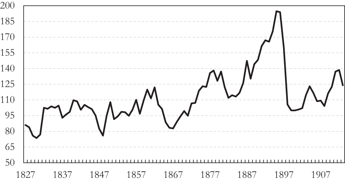
A less emphasized but important factor boosting economic growth was the significant improvement in the country’s terms of trade (the price of exports relative to the price of imports) in the second half of the 19th century, as shown in Figure 5, derived from the online appendix of Absell and Tena-Junguito (Reference Absell and Tena-Junguito2018). Indeed, measured from its trough in 1867 to its peak in 1895, Brazil’s terms of trade more than doubled during the second half of the century, increasing at an extraordinary rate of 3.1% per year.
Brazil’s terms of trade, 1827–1913 (1900 = 100).

Bacha and Bonelli (Reference Prados De La Escosura2016, pp. 163–165) demonstrate the critical role that the terms of trade had on Brazil’s total factor productivity growth in the 1980–2014 period. Greater volumes of efficiency-improving imported intermediate goods would be the transmission mechanism leading from better terms of trade to higher domestic productivity growth. It stands to reason that productivity growth would be even more dependent on the purchasing power of exports in 19th-century Brazil.
4.2. The first half of the 19th century
In his influential book on Brazilian economic history, Celso Furtado argued that the country’s per capita GDP did not increase in the first half of the 19th century. He thought, in fact, that it would have probably decreased. His argument is based on the idea that GDP growth at the time depended entirely on the growth of exports; with then available data, he supposed that the sterling value of exports had grown at a yearly rate of 0.8% in the 1800–1850 period, while the rate of population growth was 1.3%. Furthermore, terms of trade would have fallen close to 40% between 1821–1830 and 1841–1850 (Furtado, Reference Furtado, Aguiar and Drysdale1963: Ch. 19). Leff (Reference Leff1982: pp. 39–40) also mentioned the slow growth of exports, in support of his thesis of near stagnation in the 19th century.
As we have already stressed, in a recent review of Brazilian trade statistics for the 1821–1913 period, Absell and Tena-Junguito (Absell and Tena-Junguito, Reference Absell and Tena-Junguito2016, Reference Absell and Tena-Junguito2018) showed, on the contrary, substantial export growth in the 1821–1850 period, averaging 3.5% per year, while the population was growing at 1.5% (IBGE—Fundação Instituto Brasileiro De Geografia E Estatística, 1990: p. 30). In the entire 1821–1900 period, the average rate of export growth was 2.7%. From 1827–1831 to 1846–1850, the terms of trade increased about 15%, a yearly average of 0.8%.Footnote 17
There are also indications that the rapid expansion of coffee during this period led to significant productivity gains. The proportion of coffee exports in total export value jumped from 21% in 1821 (when sugar was the main export item), to 44% in 1850–1851, with sugar now in a distant second, making up only 23% of total export value (data from Absell and Tena-Junguito, Reference Absell and Tena-Junguito2016, Supplemental Material). Such inversion probably had a positive effect on output value per capita, as suggested by data from a large sample of farms in São Paulo province—where coffee spread rapidly along the Paraíba Valley, in the period—showing that the value of production per worker was 52% higher in coffee than in sugar (cf. Luna and Klein, Reference Luna and Klein2018, Table 1.1). All things considered, it can be said that external trade favoured income growth in the first half of the century.
Moreover, the notion that income growth during the period could only be derived from the export sector is no longer tenable. In recent decades, there has been growing evidence of significant domestic trade flows, particularly toward the city of Rio de Janeiro. In the 18th century, Rio, the only important port in the Central South, had become a hub for export and import trade after the discovery of gold and later diamonds in the neighbouring province of Minas Gerais. The transfer of the colonial capital from Bahia to Rio in 1763 probably enhanced economic activity in the city.
The importance of export trade via Rio increased with the “agricultural renaissance” of the last decades of the 18th century, favoured by increased prices for agricultural commodities as a result of interrupted supplies from North and Central America, caused by the destructive 1791–1804 revolution in Haiti—a major supplier of sugar and other agricultural products—and the United States war of independence (Alden, Reference Alden and Bethell1984: p.627ff). Brazilian exports of sugar, rice, cotton, and other agricultural products experienced a revival during this period. The growing sugar production in the northern part of the Rio de Janeiro province was essential for the Rio export trade.
On the other hand, the supply of basic food items to the city of Rio, such as beans and manioc, fell significantly as planters in the neighboring area turned to producing more lucrative exportable items such as rice and indigo. Consequently, providing agricultural production from Minas Gerais became important (Brown, Reference Brown1986: p. 56).
As Martins (Reference Martins2018) observed, the gold and diamond boom in Minas Gerais in the 18th century diverted many historians’ attention from the fact that, as mining prospered, agricultural production in the province increased significantly. Mining activity led to an intense influx of migrants into the province. The rapid rise in demand, especially for food products, was met, as stressed in the literature, by trade from other regions in Brazil (for instance, Furtado, Reference Furtado, Aguiar and Drysdale1963: Ch. 3).
However, more recent research on the sources of supply for the mining region, as Zemella (Reference Zemella1990) has shown, indicates that it increasingly came from inside the region itself. Prado (1971[Reference Prado and Macedo1942]: Ch. 3, 10) had already noted that as early as the 1760s, Minas sent food commodities to Rio de Janeiro and São Paulo. A long-held belief that mining and agriculture were incompatible (Antonil, 1982[Reference Antonil1711]: p.169; Furtado, Reference Furtado, Aguiar and Drysdale1963: Ch. 15) proved to be incorrect: Costa Filho (Reference Costa Filho1963: pp.159 ff), for instance, mentioned various “mixed farms” in Minas Gerais, where mining, agriculture, and cattle-raising coexisted in the 18th century.
As noted by Maxwell (Reference Maxwell1973: p. 88), such coexistence was facilitated by the Portuguese Crown’s mining rights concession system; these rights were frequently granted in land tracts that had previously been given away for agricultural purposes (the so-called sesmarias). Many authors have documented the diversity of productive activity in 18th-century Minas Gerais (see references in Martins, Reference Martins2018: pp. 508 ff). The development of non-mining production was facilitated by the fact that the Portuguese authorities, while strictly controlling and regulating activities related to gold and diamonds, granted considerable freedom to other pursuits—in which the majority of the population was engaged (Holanda, Reference Holanda and Holanda1985: pp. 289, 294–95).
In a pathbreaking paper, Martins Filho and Martins (Reference Martins Filho and Martins1983) argued that Minas Gerais in the 19th century was a slave-based economy that produced essentially for the domestic market, primarily on small or mid-sized farms—arguing also that it would be the sole example of such a productive structure in the Americas. The critical point is that, at the time, Minas Gerais was undoubtedly a major supplier of consumer goods for the domestic market.
Such supply gained importance after 1807, when, fleeing from the invading Napoleonic troops, the Portuguese court relocated to Rio de Janeiro, accompanied by a large entourage (comprising nearly 15,000 people), mostly wealthy aristocrats, bureaucrats, and merchants. The city of Rio was transformed into “the most important consumption center of south-central Brazil [and] the center of an internal trade network in which hinterland areas produced for the city’s population consumption” (Brown, Reference Brown1986: pp. 61–62). As shown in detail in Brown’s study, Minas Gerais was Rio’s main supply source in the following years. The vast network of commerce between the interior and the capital then developed, “most [of it] in commodities intended for the domestic market” (Brown, p. 476), would also eventually involve, to some extent, more distant localities in Goiás, São Paulo and Rio Grande do Sul provinces.
Such long-distance trade was based on credit, furnished mainly through Rio de Janeiro merchants; but some Minas cities were also intermediary trading centres, which led to capital accumulation and sources of credit supply outside Rio. It also led, incidentally, to the rise of an interior elite with roots in domestic trade—sometimes very active in the politics of the agitated period around the time of the Independence in 1822 (Brown, p. 507 ff; Lenharo, Reference Lenharo1979). Some of the Rio merchants became extremely wealthy and influential in the colonial administration—and, after Brazilian independence in 1822, also influential in the first monarchical government up to 1831 (Gorenstein, Reference Gorenstein, Martinho and Gorenstein1993; Fragoso, Reference Fragoso1992).Footnote 18
Some domestic trade toward Rio involved large investments, such as the supply of 20,000 head of cattle consumed in the city every year. Cattle traders frequently had to wait for up to two years to realize their profits: animals were herded in journeys of hundreds of kilometres, after which they were kept in pastures for long periods, to rest and fatten before being sold in Rio, “the only market which could draw large number of animals from great distances” (Brown, Reference Brown1986: p. 505). The accounts of one of the major São Paulo cattle traders, the Baron of Iguape, were preserved, which allowed for a detailed examination of the activities of these merchants in the 1820s and the significant investments involved in this business (Brown, pp. 500–504).
Another factor significantly impacting Brazil’s economy was the Napoleonic Wars, which triggered a sudden increase in British traders’ interest in the Brazilian market. Immediately after arriving in Brazil, the Portuguese Prince Regent decreed in January 1808 the opening of ports to all friendly nations, ending the Portuguese monopoly of trade with Brazil. At this time, British exports were severely limited by restrictions arising from the war with France; accordingly, many British merchants saw the opening of Brazilian trade as a welcome opportunity.Footnote 19
In June 1808, the Portuguese ambassador in London called a meeting of merchants who intended to do business with Brazil; 113 London merchants joined the Association of English Merchants Trading to Brazil, organized at the meeting. In the second half of this year, the number of British merchants in Rio was larger than 100, perhaps reaching 200; the eagerness to trade was such that some of the goods brought to sell in the local market were totally inappropriate, such as ice skates (Manchester, Reference Manchester1972[Reference Manchester1933]: p. 75; Pantaleão, Reference Pantaleão and Holanda1993: pp. 73–76).
In the following years, Great Britain dominated Brazil’s imports, which was made easier by a 1810 commercial treaty signed by Portugal and Britain, largely favourable to the latter. Brazil became an important market for English manufacturers; in 1820, Brazilian purchases of British goods, mainly in Rio de Janeiro, were nearly 60% of those by the United States (Britain–U.S. trade was back to normal). Exports to Britain also increased, mostly of cotton, but much less; there were significant trade surpluses in favour of Great Britain (Manchester, Reference Manchester1972[Reference Manchester1933]: pp. 96–98).
The abolition of the British slave trade in March 1807 also had far-reaching consequences for the Brazilian economy. Before 1807, British traders largely dominated the African slave trade, an activity highly dependent on credit and vulnerable to delayed returns. The British had the great advantage due to their access to London financial and commercial institutions. After abolition, British merchants attempted various expedients to maintain their presence in the slave trade; some even relocated to foreign countries. However, the constant threat of intervention by the British Navy and courts (Eltis, Reference Eltis1987: pp. 51 ff.) was always present. However, “the supply of British goods and credit proved to be beyond the power of law to control” (Eltis, p. 58).
As stressed by Miller (Reference Miller1988), the abundance of British capital played a crucial role in facilitating the intense flow of forced African migration to Brazil in the 1810s and 1820s. Some British merchants participated in the slave trade as part of their import business in Brazil. Also, some Lisbon merchants formerly engaged in the slave trade, and having moved to Rio de Janeiro along with the royal family, became agents for the British, who supplied them with credit and trade goods to be used in slave trade with Angola (this Portuguese colony was the primary source of chattels sent to Brazil). Angola-based traders, who formerly controlled the bulk of the Brazilian slave trade, were now marginalized by the Anglo-Portuguese merchants; Brazilian traders faced a similar fate (Miller, Reference Miller1988: p. 505 ff; Klein, Reference Klein1978: pp. 82–83).
Recently published data on the slave trade allow a more precise evaluation of the extraordinary flow of enslaved Africans to Brazil in the first half of the 19th century.Footnote 20 From 1800 to 1850 (when the slave trade was abolished in Brazil), close to 2.1 million forced migrants from Africa entered the country, more than 40% of the total registered during the three centuries of the slave trade into Brazil (4.9 million). In the 1810s and 1820s, when close to 50,000 coerced laborers entered the country each year, trade was especially profitable, which explains “the eagerness of Brazil-based metropolitan traders to gain ownership of the slaves in those decades” (Miller, Reference Miller1988: p. 513).
The monetary significance of such a large inflow may be gauged by ascribing an average price to the forced migrants. In the 1820s, when the slave trade brought to Brazil reached its peak (close to 524,000 Africans), an average of 210 mil-réis is suggested in Bergad (Reference Bergad1999, pp. 268–69).Footnote 21 At this price, the total value of the 524,000 forced migrants, converted into sterling pounds (£ 17.3 million), is a sizeable proportion (29.6%) of total merchandize imports in the decade (£ 58.4 million).Footnote 22 It is clear that investment in the slave trade toward Brazil was considerable in the period (and also that a large portion of the total import trade went unrecorded).
Which activity demanded so many enslaved workers in the first half of the 19th century? Coffee cultivation rapidly expanded during this period, especially after 1820 (Bacha, Reference Bacha, Martins and Johnston1992); this suggests that coffee farms were the leading destination for these workers. This suggestion was likely reinforced by the fact that Rio was the port of entry for most incoming chattels at the time, and Rio de Janeiro province was, then, the main coffee-producing region. In fact, the Brazilian slave trade in this period is often related to coffee in the literature (Miller, Reference Miller1988: pp. 459, 493; Klein, Reference Klein1999: p. 41).
However, official registers of domestic slave trade between Rio de Janeiro city and the provinces tell a different story for the 1809–1833 period.Footnote 23 In the 1821–1830 decade, the leading destination was the province of Minas Gerais (41% of the total); 34% went to the Rio de Janeiro province, 15% to São Paulo province, and 10% to other provinces. In the two decades together (1811 to 1830), Minas and Rio provinces received approximately 80% of the arriving slaves (equally divided between the two), while 12% went to São Paulo.
Those numbers substantiate the early contention, in Martins Jr. and Martins (Martins Filho and Martins, Reference Martins Filho and Martins1983), that the Minas Gerais province was a large importer of enslaved Africans in the first half of the 19th century, and a significant supplier of agricultural goods to the domestic market. Contrary to a then-prevailing notion, according to which Minas was, in the period, an exporter of forced labor to the coffee-growing areas, as the ending of the mining boom would have caused the province to have an “excess” of enslaved workers (cf. Furtado, Reference Furtado, Aguiar and Drysdale1963: Ch. 20).
Thus, it is clear that production and trading activity geared to domestic consumption, especially after 1807, was very significant. Rio de Janeiro was a major source of demand for this production, and Minas Gerais was probably a significant source of supply.
In conclusion, there is much evidence of a favorable climate for economic growth in the first half of the 19th century. According to Absell and Tena-Junguito, exports showed a healthy increase, especially in the 1821–1840 period (4.2% per year, in sterling value). Such an increase was probably associated with productivity gains. There was heavy investment in the African slave trade, probably financed by British traders, and a large proportion of the increase in the enslaved labor force was linked to an expansion of goods produced not for export but for the domestic market. There are no signs of stagnation, as most of the literature, until now, has supposed.
5. Comparison of Brazil’s performance with other countries in the 1800s
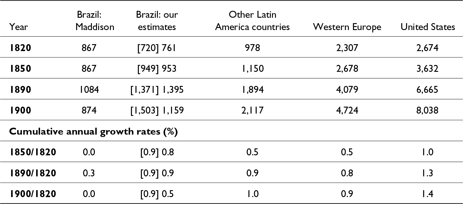
In Table 2, we compare the evolution of Brazil’s per-capita GDP with other countries/regions in the 19th century. For Brazil, we list the MPD estimates and our own—the latter converted into 2011 U.S. dollars with the per-capita GDP value of the MPD in 1900 corrected according to Bacha, Tombolo and Versiani (Reference Versiani, Bielschowsky, Boianovsky and Coutinho2023) (henceforth, BTV).Footnote 24
Per-capita output in the 1800s: Brazil and other countries (2011 USD)

Source: Brazil/Maddison, W. Europe, and US: MPD (Maddison Project Database (MPD), 2020). Other L.A., estimated from L.A.’s and Brazil’s GDP per capita and population in MPD (Maddison Project Database (MPD), 2020). Brazil/Our estimates: in 1900, $874 from MPD (Maddison Project Database (MPD), 2020) plus 32.6%; in brackets: trend values according to the Theil-Sen estimator.
According to the MPD, the value of Brazil’s per capita GDP (in 2011 USD) was $1,585 in 1980. Taking this value as given and using the yearly growth rate from 1900 to 1980 calculated by BTV, we conclude that Brazil’s per capita GDP (in 2011 USD) was $1,159 in 1900, a value 32.6% higher than the MPD’s estimate of $874.
The countries/regions of comparison are other Latin American countries, Western Europe, and the United States—with data from the MPD.Footnote 25 The table lists estimates for 1820, 1850, 1890, and 1900. In the case of our estimates for Brazil, we list both our point estimates and, in brackets, the values along the trendline, according to the Theil–Sen estimator. The last three rows present the cumulative annual growth rates for relevant subperiods.
The figures in the table confirm the exceptionalism of U.S. growth, particularly in the second half of the 19th century. According to our estimates, Brazil’s performance is on par with other Latin American countries and Western Europe before 1890. That is, our series of real per-capita output is consistent with the performance of Latin America in the 19th century, according to the Maddison Project database. Our economic history arguments suggest that it is implausible that Brazil’s economy performed so differently from the rest of Latin America, as the Maddison Project indicates.
According to our proposed figures, Brazil performed slightly worse than the United States in the period from 1820 to 1850. This finding contrasts with previous studies asserting that Brazil’s economy stagnated in the first half of the century. However, our figures align with regional economic trends in the U.S.: economic historians agree that the South’s slave-based economy grew at a similar rate to the rest of the country in the 19th century, before the Civil War.Footnote 26 In both these slave-based societies—Brazil’s and the U.S. South’s—the robust economic growth in the early 19th century seems related to the interplay between the vigour of world demand and the sluggishness of alternative supply sources for the agricultural goods they produced. In the U.S. South, productivity growth was closely tied to innovations in cotton production and processing technologies. In Brazil, we believe productivity growth has been driven by the shift from sugar to coffee production.
Brazil was subject to a perfect storm in the last decade of the 19th century. First, there was an inflation burst, a consequence of the erratic monetary policies adopted in the first years of the Republican period, which began in November 1889. A sharp fall in the exchange rate followed, aggravated by the sudden stop of capital inflow caused by the international Panic of 1890; the average sterling value of the mil-réis in 1892 was less than half what it had been in 1889 (IBGE—Fundação Instituto Brasileiro De Geografia E Estatística, 1990: pp. 592–3). This increased the burden of external debt payments on government expenditures; the federal budget was further burdened by heavy military expenses related to rebellions in Rio Grande do Sul (1893–95) and Bahia (1896–97). The government’s difficulties and the collapse of the coffee market in 1896 led to a foreign debt restructuring in 1898, followed by the highly contractionary monetary policies of Finance Minister Joaquim Murtinho in the last two years of the century (cf. Franco, Reference Franco and Abreu2014).
This perfect storm generated a sharp aggregate demand shortfall; however, there are various indications that the real economy was expanding fast in the period. In 1894, after the end of the speculative bubble, it was already noted “the obvious disparity between the poor situation of the Treasury and monetary management, and the economic situation of the country […]. Despite all wild speculation in the stock exchange, Brazilian productive activities kept progressing” (Calógeras, Reference Calógeras1960[Reference Calógeras1910], p. 279, our translation). And the factors that favoured Brazilian economic growth in the second half of the nineteenth century were conspicuously present in the last decade: from 1891 to 1900, 1.1 million immigrants entered the country (Merrick and Graham, Reference Merrick and Graham1979, p. 37); the extension of the railroad network increased 45% (IBGE—Fundação Instituto Brasileiro De Geografia E Estatística, 1986, p. 41); industrial machinery imports were 61% greater than in the previous decade (Suzigan, Reference Suzigan1986, app. 1); 22 new cotton textile mills were established (Versiani, Reference Versiani1979, app. A); installed capacity of the (nascent) waterpower-generated electricity increased tenfold (Dean, Reference Dean and Holanda1997, p. 255).
These are the reasons why our estimates in Table 2 display a marked difference in 1900 between the trend (or potential) per-capita GDP of US$1,503 and the actual per-capita GDP of US$1,159. Brazil’s sharp acceleration in the subsequent decades suggests that the trend estimate is not a statistical artefact (cf. Haddad, Reference Haddad and Neuhaus1980).
6. Conclusions
“I tried to trace the history in quantitative terms, whenever possible, and I hope that many proxy estimates that I had to use will be improved by Brazilian specialists”. These were the words of Raymond W. Goldsmith in the preface to his solitary tour de force to provide a year-by-year quantitative analysis of Brazil’s economic growth since 1850 (Goldsmith, Reference Goldsmith1986, Preface; our translation). Goldsmith’s estimates became the basic reference for estimating Brazil’s GDP growth in the second half of the 19th century and were adopted by the MPD.
For 1800, 1820, and 1850, the Maddison Project continued to adopt a proposal by Prados De La Escosura (Reference Prados De La Escosura2009, p. 301, Table 6), which suggests that Brazil’s per-capita income was constant in the first half of the 19th century. This stagnation hypothesis has become consensual in the literature, as exemplified by Abreu, Lago, and Villela (Abreu et al, Reference Abreu, Lago and Villela2022, p. 21).
This paper builds on Tombolo (Reference Tombolo2013), summarized in Tombolo and Sampaio (Reference Tombolo and Sampaio2013), to provide new estimates for Brazil’s per-capita GDP growth from 1820 to 1900. The basic method follows that of Goldsmith (Reference Goldsmith1986): lacking information on production volumes, the alternative is to aggregate yearly monetary series related to nominal per-capita GDP (namely, money supply, government income and expenditure, exports and imports of goods) and deflate the aggregate by available price indices, to obtain proxies for real per-capita GDP.
Our series are similar to those used by Goldsmith. The primary difference in our monetary series is that it extends back to 1820. They are newer—particularly for exports and imports of goods (from Absell and Tena-Junguito, Reference Absell and Tena-Junguito2016, Reference Absell and Tena-Junguito2018), as well as central government income and spending (from Carrara, Reference Carrara2022). Furthermore, they are aggregated according to a methodology developed by Tombolo, which respects their relationships with nominal GDP in the 20th century.
Our price deflator series also used a new and only truly reliable price index for the latter part of the 19th century (Catão, Reference Catão1992), while estimating the inflation rate for the rest of the century with a combination of the two next-best indices (Lobo et al, Reference Lobo, Canavarros, Feres, Gonçalves and Madureira1971; Buescu, Reference Buescu1973), which is respectful of their relationships with the Catão index in the 1871–1897 period.
The alternative that we consider best for Brazil’s real per-capita GDP from 1820 to 1900 has two characteristics. First, the trend is clearly positive. Second, the series is quite volatile, with periods of expansion alternating with periods of contraction of varying magnitude and duration. This volatility makes it difficult to distinguish signal from noise on a year-to-year basis, which is why we focus on the trend line. This line has a slope indicating an annual growth rate of 0.9% for Brazil’s per-capita GDP between 1820 and 1900, with a 95% confidence interval ranging from 0.6% to 1.2%. We identified no structural breaks in the series, indicating that the same trend growth rate applies for both the 1820–1850 and 1850–1900 periods.
Our results are less surprising for the second half of the 19th century than they are for the century’s first half, for Furtado (Reference Furtado, Aguiar and Drysdale1963, Ch. 25) had long claimed that Brazil grew handsomely from 1850 onward. In the paper, we show that it was only because of the choice of inappropriate price deflators that Goldsmith found lower growth rates for this period than our own estimates. For the first half of the century, however, Furtado assumed that the country’s economy stagnated, if not actually shrank, in absolute terms. We argue that Furtado inferred GDP’s growth from the stagnant behavior of per-capita exports, a series that has recently been subject to substantial upward revision (Absell and Tena-Junguito, Reference Absell and Tena-Junguito2016).
To support our proposed estimate for Brazil’s per-capita GDP growth rate in the first half of the 19th century, we provide historical evidence of not only substantial export-oriented growth but also of domestic commerce as a significant source of income growth during the period. There was heavy investment in the African slave trade, and a sizable proportion of the net increase of the enslaved labor force was linked to production for the domestic market.
The paper concludes by comparing Brazil’s economic performance in the 19th century with that of other Latin American countries, Western Europe, and the United States. The figures confirm the exceptionalism of US growth, particularly in the second half of the century. However, Brazil’s per-capita GDP growth was on par with other Latin American countries and Western Europe up to 1890. It was only a sharp, albeit temporary, contraction in the late 1890s that dulled Brazil’s performance at the century’s end.
Did Brazil stagnate in the 19th century? Our proposed answer is No, it did not. Brazil’s per-capita GDP growth rhythm was apparently quite normal for the general pattern of the century.
We reiterate that this is far from a perfect proposal; it is the result of a reasoned exploration of alternatives, based on which we offer the best option according to our research. We consider our new series crucial because it indicates positive economic growth, particularly during the period up to 1850, in better agreement than previous studies with the economic history of the period. With this approach, we hope to contribute to enhancing our existing knowledge and exploring novel avenues of research on Brazil’s economy in the 19th century.
Supplementary material
The supplementary material for this article can be found at https://doi.org/10.1017/S021261092510058X.
Appendix
A1. Nominal per-capita GDP
To estimate nominal per-capita GDP for the 19th century, we ran a regression for the 1900–1947 period, with the log of the nominal per-capita output (from Haddad, Reference Haddad1978) as the dependent variable. As independent variables the logs of an arithmetic mean of exports and imports of goods in national currency (which we denominate as “foreign trade index”), the arithmetic mean of central government revenues and expenditures (which we denominate as “government budget”), and a money-supply index, all expressed in per-capita terms.
Haddad’s nominal output is available only from 1908 onwards. To obtain a nominal GDP series for the entire 1900–1947 period, we multiplied Haddad’s real output series by the Catão (Reference Catão1992) wholesale price index and linked the results to Haddad’s nominal output in 1908. The variables used in the model are expressed in current prices with base year 1900 = 100.
Our estimates of the Brazilian population for 1820-1915 are from Mortara (Reference Mortara1941), and for 1916–1947, from Ipeadata (2022). We use Mortara’s data through 1915, taking into consideration the author’s observation that the 1900 Census, used by Ipeadata, underestimated the population in residence.
For the period 1821–1913, we use the exports and imports series of Absell and Tena-Junguito (Reference Absell and Tena-Junguito2018, online appendix), converted from British Pounds to mil-réis using the official exchange rate in Brazil (1917, p. 243). We used Menezes’ (Reference Menezes2010) series of Brazil’s exports and imports, chained to Absell and Tena-Junguito, for 1820. For the period 1914–1947, we utilised the official series of exports and imports in local currency provided by IBGE (1990, pp. 570–571). The official series was linked to the Absell and Tena-Junguito series in 1913.
The series of the central government’s revenues and expenditures is the revised series of Carrara (Reference Carrara2022) for 1820–1898. In a personal communication, Carrara kindly provided us with the data for 1899 and 1900. By official decree of October 8, 1828, the fiscal year began on July 1 and ran through June 20 of the following year. The equivalence between the calendar and the fiscal year was reestablished in 1888. We calculated the arithmetic mean between two consecutive fiscal years to align the calendar and fiscal year. The series of central government’s revenues and expenditures for the 1901–1947 period is from IBGE (1990, pp. 533–539).
The monetary series is from Peláez and Suzigan (Reference PelÁez and Suzigan1981), as reproduced without moving average adjustments in IBGE (1990, pp. 533–539). This money supply series was constructed as follows: currency issued from 1820 to 1838, M1 plus demand and term deposits at Banco do Brasil from 1839 to 1851, and the M2 monetary aggregate from 1852 to 1947. We joined the currency issued series to that of M1 plus demand and term deposits at Banco do Brasil in 1839.
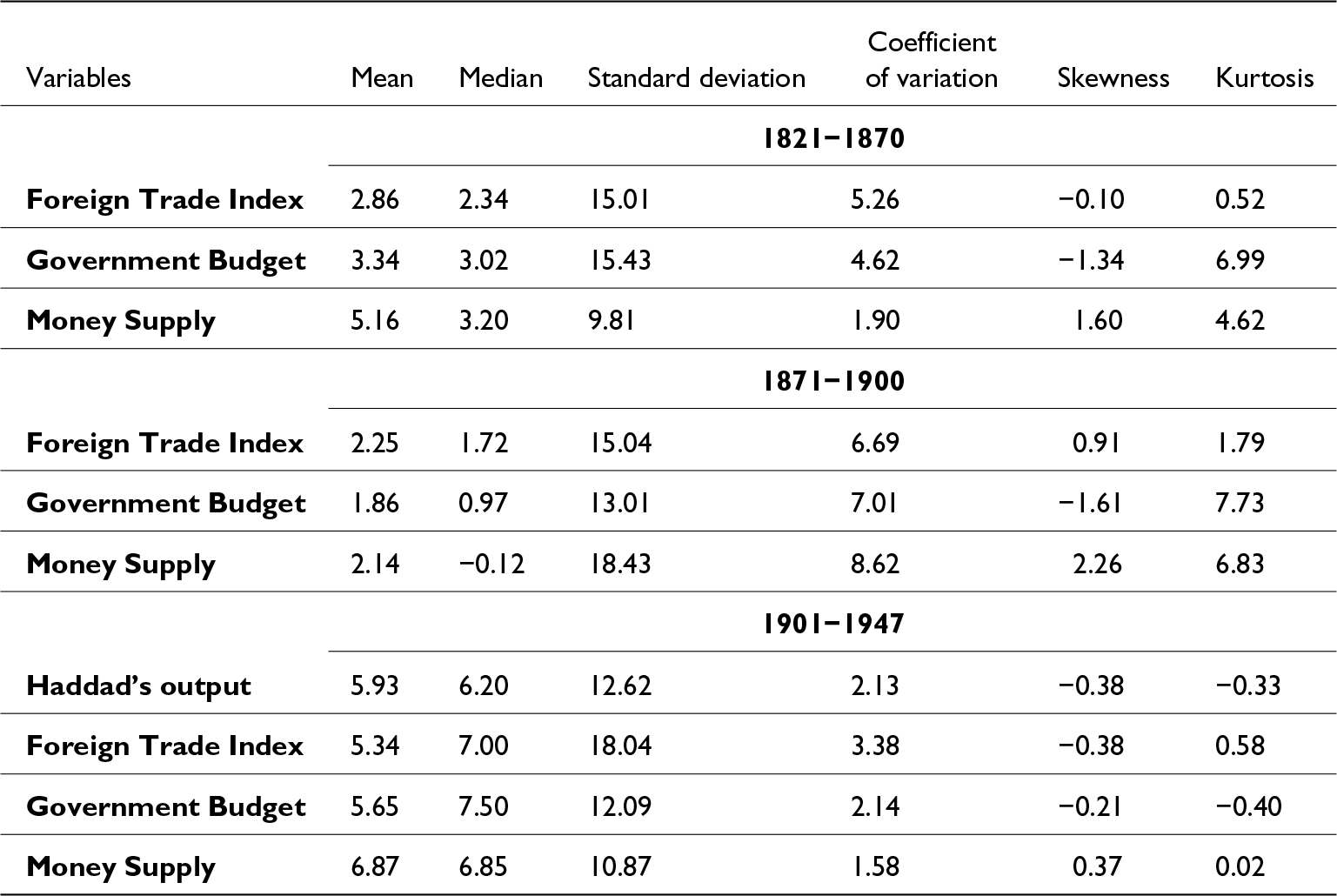
In Table A1, we present the descriptive statistics of the variables expressed as annual percentage changes (log differences). We divided the sample into three parts: 1821–1870, the period of Independence until the end of the Paraguayan War; 1871–1900, the period after the War until the end of the 19th century; and 1900–1947, which was the sample used in the regression of nominal output per capita.
Descriptive statistics of the variables - annual percentage changes*

Note: *percentage changes measured in log differences.
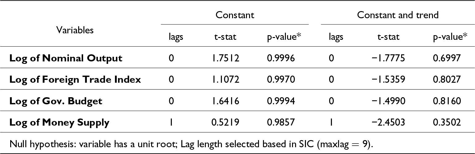
In Table A2, we apply an augmented Dickey–Fuller test (ADF) to the series to test the null hypothesis that a unit root is present in the time series samples. The high p-values obtained confirm that all series have a unit root.
Augmented ADF test, variables in levels in per capita terms: 1900-1947

Note: MacKinnon (Reference Mackinnon1996) p-values.
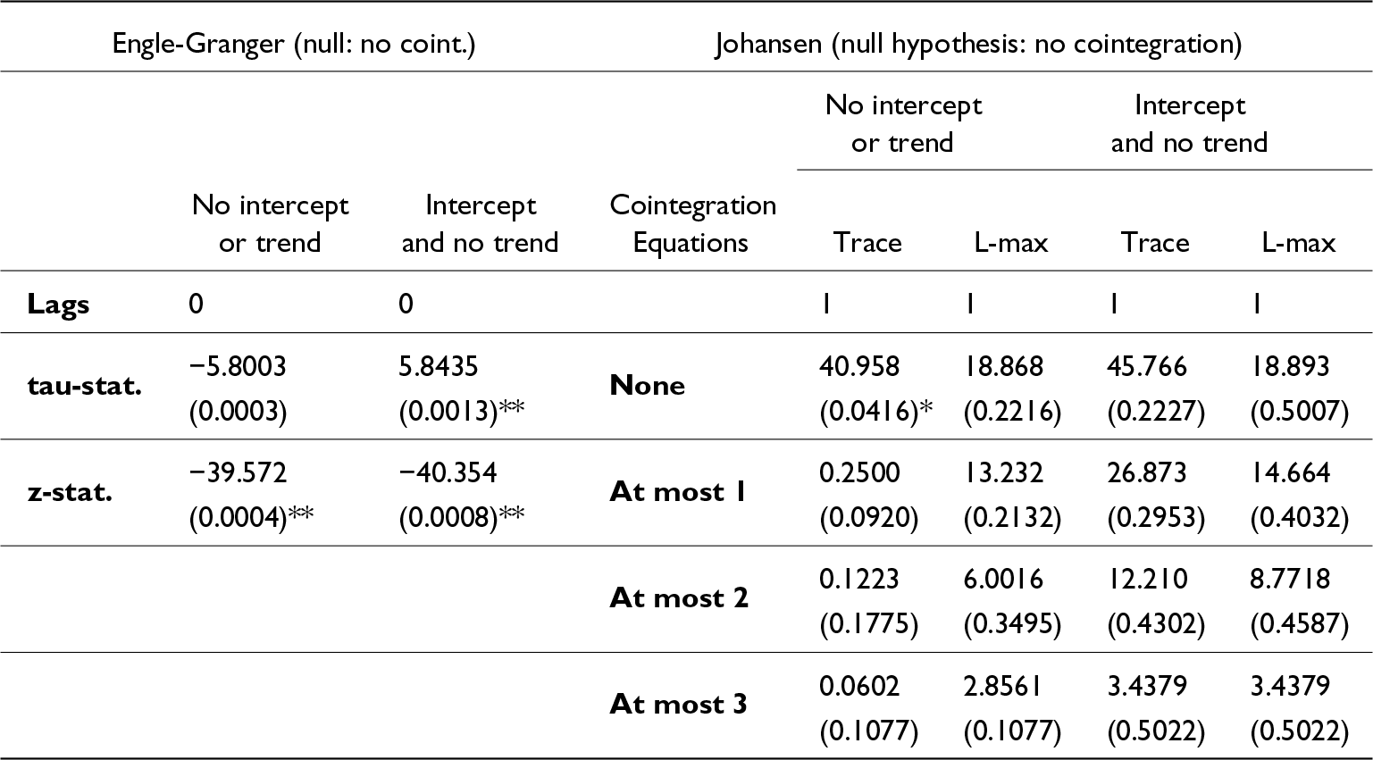
In Table A3, we present cointegration tests. The Engle-Granger test consists of a unit root test on the residuals of the cointegrating regression shown in Table A4. The Engle-Granger test rejects the null hypothesis of a unit root in the residuals (in both variants, with and without an intercept). It therefore indicates the possible presence of cointegration among the variables. Johansen’s test rejects the null hypothesis of no cointegrating equations in the no-intercept-no-trend specification. In the estimated equation in Table A4, the intercept is statistically insignificant, consistent with the Johansen test in the no-intercept-no-trend specification.
Cointegration tests of Engle-Granger and Johansen: 1900-1947***

Notes: * Denotes rejection of the hypothesis at the 5% level and ** at the 1% level. *** p-values in brackets, MacKinnon (Reference Mackinnon1996) p-values in the Engle-Granger test and MacKinnon, Haug and Michelis (Reference Mackinnon, Haug and Michelis1999) in the Johansen test.
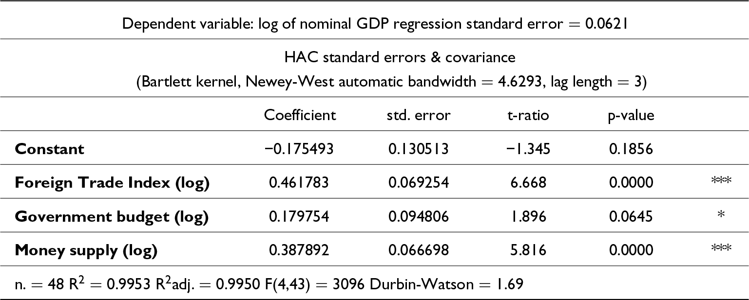
Nominal per-capita output regression: 1900–1947

Note: * Indicates significance at 10%, ** at 5%, and *** at 1%.
Results of the nominal per-capita output regression are presented in Table A4.
As expected in a cointegrating regression, R2 is high, and all the coefficients of the regression are significant. They add up to just greater than one (1.0294), and a restriction that they must add up to one (1.00) is not rejected by a Wald F test with a p-value of 30.73% (F-statistic = 1.0667, degree of freedom = 1,44). Using the coefficients of the regression in Table A4, we distribute them by the pro rata method so that the variables weights add up to exactly 1. Using the calculated weights, we construct a Laspeyres index for nominal per-capita product with 1900 as the base year, ranging from 1820 to 1900:
 \begin{equation*}\mathit{Y_t^n} = 100 \times \left( {0.448582 \times {{\widehat {\mathit{FT}}}_t} + 0.174615 \times {{\widehat {{\mathit{GB}}}}_t} + 0.376803 \times {{\widehat{\mathit{M}}}_t}} \right)\end{equation*}
where the hats on top of the variables indicate the (gross) percentage change between year  $t$ and year 1900;
 $\mathit{Y}_t^n$ is the nominal output;
 $\mathit{F{T}_t}$ is the foreign trade index obtained by the arithmetic mean of exports and imports;
 $\mathit{G{B}_t}$is the “government budget” obtained by the arithmetic mean of government expenditures and revenues; and
 ${\mathit{M}_t}$ refers to a series of money supply. All variables are in per-capita terms. In the interval between 1890 and 1892, we excluded the money supply from the construction of the nominal per-capita product index to avoid the distorting effects of the huge monetary expansion that occurred in the transition from monarchy to republic.
A2. Output deflator
The most rigorous Brazilian price index for the latter part of the 19th century is Catão (Reference Catão1992). This author presented “a new wholesale price index based on a much broader basket of goods and a macroeconomically representative weighting system derived from the first national production census in 1919” (Catão, p. 519). Catão’s main source of data was Brazil’s most important newspaper at the time—the Jornal do Commercio—where he obtained price estimates for 30 products: beans, beer, Brazilian brandy (aguardente), butter, candles, cement, cod fish, coffee, corn, dried meat, lard, ham, Italian pasta, linseed oil, kerosene, manioc flour, matches, olive oil, pinewood, rice, salt, sugar, tallow, tar, tea, tobacco, turpentine, vinegar, wheat flour, and wine.
Although the price quotations are for the city of Rio de Janeiro, Catão believed there were strong reasons to accept such prices as representative at the national level. First, he argued that Rio was the most important Brazilian economic centre in the 19th century, supplanted by São Paulo only after the second decade of the 20th century. Second, “a rough comparison between the indices of Lobo et al. (Reference Lobo, Canavarros, Feres, Gonçalves and Madureira1971) for Rio and those of Mattoso (Reference Mattoso1978) for Salvador and Eisenberg (Reference Eisenberg1974) for Recife showed that price trends were very similar across these state capitals” (Catão, p. 521). Third, some commodities sold in Rio were, in fact, imported from other Brazilian regions. The only problem with Catão’s index was that it is available only from 1870, hence it needed to be linked to others to cover the 19th century.
Lobo et al. (Reference Lobo, Canavarros, Feres, Gonçalves and Madureira1971) is a widely used source for domestic price indices in the 19th century. She estimated three price indices based on nine food products in the city of Rio de Janeiro between 1820 and 1930: Footnote 1 sugar, rice, cod, coffee, dry meat, wheat flour, manioc flour, beans, and butter. Each index contains the same goods differing only in terms of the weights: the first index has 1856 as base-year and its weights are inferred from information in Diários da Companhia de Luz Stearica on the amounts (in Mil-réis) spent on food by workers, enslaved people, and settlers. The second index has 1919 as its base year, and the weights were borrowed from Affonseca (Reference Affonseca1919), who built a cost-of-living index for Rio de Janeiro based on his own domestic budget, a household composed of seven individuals. The third weight structure has 1949 as its base year and is derived from the Getúlio Vargas Foundation’s consumer price index.
Buescu (Reference Buescu1973, p. 233) presented an alternative price index, with a thorough investigation of price changes from 1826 to 1887. Between 1826 and 1880, he primarily determined his index through a detailed price search of classified ads in Brazil’s leading newspaper of the time, the Jornal do Comércio. For 1880 to 1887, his sources were the annual Reports of the Finance Ministry and the yearly Retrospects of Jornal do Commercio. For this last period, he collected annual price changes, whereas for 1826 to 1880, his observations are for selected years (1826, 1830, 1835, 1838, 1842, 1847, 1850, 1853, 1856, 1862, and 1870). The number and nature of products in his index changed throughout the period. On average, he collected prices for 17 products in 1826–1838; 90 in 1838–1850; 44 in 1850–1870; 24 in 1870–1875; 12 in 1875–1880; and 50 in 1880–1887. One weakness of his index is the lack of a weighting structure, as noted by Haddad and Versiani (Reference Haddad and Versiani1990, p. 135). However, he attempted to address this deficiency by indirectly weighting each product according to the number of times it appears in his samples.
Buescu’s index for Brazil begins in 1826, while his index for Rio de Janeiro spans from 1772 to 1819. It was thus necessary to link the two indices. For this, we extended the inflation rate (2.5% per year) that Buescu conjectured for Rio between 1807 and 1819 from 1819 to 1824. For 1825 and 1826, we used the rate of 7% per year that Buescu estimated for Brazil’s inflation between 1826 and 1830.
In each chapter of his book, Buescu compares his results with those of other price indexes for the respective period. Of particular interest are the comparisons he makes with the price indexes of Lobo. In general, he finds that his index shows lower inflation rates than Lobo’s. He attributes this to the fact that Lobo’s indexes are restricted to a limited number of food products, the prices of which may have risen by more than the tradable products included in his index. The larger discrepancy is in the 1850–1870 period, for which his accumulated inflation rate is 84%, whereas Lobo’s varies from 274% to 308%, depending on the weighting structure. This large discrepancy does not appear in Mattoso’s (Reference Mattoso1978) food price index for Bahia, which, according to Buescu (p. 176), rose by 90% during the period.
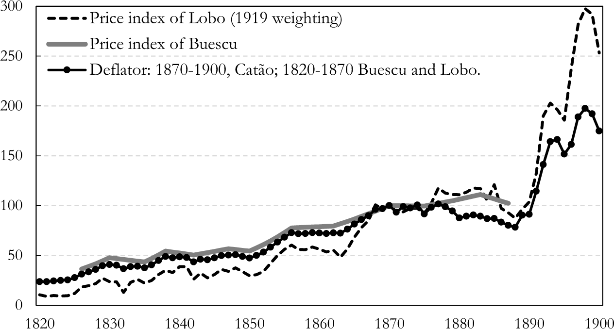
Figure A1 displays the price indices of Buescu, Catão and Lobo from 1820 to 1913 with base year 1880 = 100. From 1820 to 1845, the Lobo price index (1919 weighting) indicates a yearly inflation rate of 4.4%, and an annual rate of 4.8% between 1845 and 1870. Between 1820 and 1845, the Buescu price index shows an annual inflation rate of 2.6%; and 2.5% yearly between 1845 and 1870.
– Price indexes of Buescu, Catão and Lobo, 1820-1913 (1870 = 100)

Comparing the indices for 1870–1887, a period for which the three indices have data, the Buescu price index shows a yearly inflation rate of 0.1%, the Lobo index -0.4% and the Catão index -1.3%. The Catão index exhibits a stronger deflation in the 1870–1888 period that is not fully captured by the other indices. This fact plays a key role in explaining the paradoxical result obtained by Goldsmith which shows a negative trend in the growth of Brazilian real per-capita output between 1869 and 1900.
The Catão wholesale price index is available from 1870 to 1913, so we used it as the GDP deflator from 1870 to 1900. One could use the Lobo index to extend the Catão index backwards; however, this is a food-cost index that relies only on the prices of nine or fewer commodities. The Buescu price index, on the other hand, does not have a weighting structure but is composed of a larger sample of goods.
We adopt a compromise solution of combining the price indices of Buescu and Lobo—the latter with weights from 1919—to extend Catão’s index back to 1870. To do this, we first regress the log first differences of the Catão price index on the log first differences of the price indices of Buescu and Lobo for the 1871–1887 period. We impose the restriction that the sum of the two coefficients is equal to one to obtain appropriate weights. We also run the model imposing a zero constant to ensure the consistency of the resulting index.
Deflator regression: 1871–1887

Note: ** Indicates significance at 5% and *** at 1%.
Thus, our deflator for the 1870–1900 period is the wholesale price index of Catão (Reference Catão1992). For the 1820–1870 period, our deflator is a Laspeyres index, based on 1870, built on the price indices of Buescu (Reference Buescu1973) and Lobo et al. (Reference Lobo, Canavarros, Feres, Gonçalves and Madureira1971)—the latter with 1919 weights—linked to Catão’s wholesale price index in 1870:
 \begin{equation*}{\mathit{P}}_t = 100 \times \left( {0.716484 \times {\hat {\mathit{B}}}_t + 0.283516 \times {\hat{\mathit{L}}}}_t \right)\end{equation*}
where the hats on top of the variables indicate the (gross) percentage change between year  $t$ and year 1870;
 ${\mathit{P}_t}$ is our proposed output deflator,
 ${\mathit{B}_t}$ is the Buescu price index and
 ${\mathit{L}_t}$ is the Lobo price index. This Laspeyres index is then spliced into the Catão index in 1870 to extend it back to 1820. This is the price index that we use as a deflator of nominal per-capita GDP in the 19th century.
Goldsmith constructed his deflator based on the average of four price indices: Buescu (Reference Buescu1973), Lobo et al. (Reference Lobo, Canavarros, Feres, Gonçalves and Madureira1971), Onody (Reference Onody1960), and Vieira (Reference Vieira1947). We did not consider either Onody’s or Vieira’s price indices because they suffer from serious shortcomings. Onody’s price index is made of 18 imported goods retrieved from the government’s customs tariff schedules (for some years, the number of goods is reduced to 10). It is available only for selected years scattered through the 19th century (1829, 1834, 1844, 1857, 1860, 1874, 1881, 1887, 1896, 1900). According to Versiani (Reference Versiani, Bielschowsky, Boianovsky and Coutinho2023), another major weakness of Onody’s price index is that the prices in the government tariff schedules were updated with lags to market prices, in addition to frequent tariff reforms, which made tracking prices difficult. Moreover, the construction of official prices was heavily influenced by importers’ lobbies and, in the last decades of the century, by protectionist interests. That is, the relationship between official and market prices was precarious.
Vieira’s price aggregate is also problematic. It consists of a weighted mean of yearly unit values (total exports in Mil-réis divided by export volumes) of Brazil’s nine most important export commodities, from 1821 to 1940. As such, it cannot be classified as an accurate price index, since it is not composed of homogeneous products and suffers from a quality bias. Moreover, the underlying official export prices were challenged by Absell and Tena-Junguito (2018), who reported dramatic changes in their estimated values.
A3. Real per-capita output: structural break tests
To search for possible multiple breakpoints in the series, we apply the Bai-Perron (Reference Bai and Perron2003) tests, as shown in Table A6. The “Sequential” Bai-Perron test begins by testing the null hypothesis of zero versus one breakpoint (0 vs. 1). If the null hypothesis is not rejected, the following hypothesis tested is one vs. 2, and so on, up to the maximum number of breaks allowed. Already at the beginning, the test does not reject the null of 0 vs. 1 breakpoint at a significance of 5%, and the Scaled F-statistic, 4.76, is smaller than the 5% critical value of 11.47.
Multiple breakpoint tests, sample = 1820-1900, n = 81

Notes: * Significant at the 0.05 level; ** Bai-Perron (Reference Bai and Perron2003) critical values; *** minimum information criterion values displayed with shading.
Likewise, we perform a Bai-Perron of L globally optimised breaks against the null of no structural breaks (L vs. 0 breaks). The test identifies two possible sets of breaks at a 5% significance level. A sequence of three breaks: 1847, 1864 and 1878; and another sequence of five breaks: 1832, 1844, 1857, 1870 and 1889. The five-break-point hypothesis has the largest F-scaled statistic among the Bai-Perron tests and could be chosen. To test the two variants of the Bai-Perron test, we use the Schwarz and the Liu-Wu-Zidek information criteria to select the number of breaks. In Table A5, both the Schwarz and the LWZ information criteria select zero breaks (at 5% of significance) as done by the Bai-Perron sequential test.