


1. Introduction
The timing of retirement is a major determinant of lifetime earnings and a crucial factor in financial security at older ages. However, people face uncertainty about the timing of their retirement and make consumption and savings decisions based on their expectations. One prominent source of uncertainty relates to the evolution of health. While declines in health may decrease work capacity and prevent people from working as long as they had planned, some health conditions may lead to greater medical expenses, generating an incentive to work longer (especially when health insurance is tied to employment). Of course, the relative strength of these competing forces is likely to depend on the specific nature of the health condition. Therefore, an important task for empirical work is to provide evidence on how changes in health influence retirement expectations and to document how the magnitudes of the effects vary across different types of health risks.
Yet, providing causal evidence on how health affects retirement expectations is difficult. There are two key challenges. One is identification. Correlations between health and expectations may not reflect causal relationships because of concerns like omitted variable bias. For example, unobserved preferences for leisure can influence how long people plan to work, but also health behaviors and investments. The other challenge is data availability. The Health and Retirement Study has served as a dominant source of data on retirement expectations for decades, but early waves of the survey collected information on these expectations only for people currently working, which is a selected sample. This data limitation prevented researchers from analyzing expectations for an important group, those whose health prevented them from working when they were surveyed.
In this paper, we use an event study framework and updated data to overcome these challenges, providing new causal evidence on how health impacts retirement expectations. For identification, we leverage the quasi-random timing of various health shocks. For each health shock of interest, we focus on a group of people who all experience the same shock and then track the evolution of retirement expectations around the timing of the shock. Our approach thus avoids potentially problematic comparisons between people who experience declines in health and people who do not. Moreover, recent waves of the Health and Retirement Study ask both current workers and non-workers about their retirement expectations. We avoid sample selection concerns by conducting our event study analysis using these updated data.
We study several different analysis samples, one for each health shock of interest. Our data allow us to study shocks defined using both subjective and objective health measures. For each shock, we define a sample of people between the ages of 50 and 60 who experience the shock and analyze how their self-assessed probabilities of working past older ages evolve before and after the shock. Our primary outcome variables are the self-assessed probabilities of working past 62 and 65, but we also study the probability of working past 70 when possible. The first two outcomes are especially relevant for policy because they correspond to eligibility ages for Social Security retirement benefits and Medicare, respectively.
We begin by studying declines in subjective health. Specifically, we estimate the effects of a decline in self-reported health status from excellent, very good, or good to fair or poor. The event study estimates reveal flat pre-shock trends in expectations before the health status decline and large decreases in the likelihood of working past 62 and 65 after the shock. Our preferred specification indicates that a decline in health status reduces the likelihood of (i) working past 62 by 4.1 percentage points, an 8.9 percent decrease from the baseline mean of 46 percent, and (ii) working past 65 by 4.5 percentage points, a 13.6 percent decrease.
Next, we study declines in objective health, focusing on two main measures. First, we estimate the effects of overnight hospitalizations. The signs of the estimates suggest that hospitalizations lead people to expect to retire earlier, but the estimates are not statistically different from zero. Second, we estimate the effects of a newly diagnosed health condition. In the spirit of Hosseini et al. (Reference Hosseini, Kopecky and Zhao2022), we construct a summary measure equal to the total number of conditions a person has ever experienced, using variables for diagnoses of arthritis, cancer, diabetes, heart attacks or heart disease, high blood pressure, lung disease, psychiatric conditions, and strokes. We then define a new diagnosis shock as an increase in this summary measure. We find that new diagnoses lead to statistically significant decreases in the likelihood of working past 62 and 65 that amount to 2.8 and 1.7 percentage points, respectively, which are decreases of 6.7 and 5.9 percent when compared to the means.
We then unpack this result on new diagnoses by studying separate events for each of the eight health conditions in our summary measure. Some, but not all, of these conditions significantly impact retirement expectations. For example, we find clear evidence of decreases in the likelihood of working past 65 after diagnoses of cancer and strokes. The point estimates for these shocks indicate sizable reductions in the probability of working of 20.0 and 44.6 percent when compared to the means. In contrast, we find little to no evidence that new diagnoses of diabetes and high blood pressure lead to changes in retirement expectations.
Our study relates most closely to papers that analyze health and retirement expectations (Dwyer and Mitchell, Reference Dwyer and Mitchell1999; McGarry, Reference McGarry2004; Gupta and Larsen, Reference Gupta and Larsen2010; Munnell et al., Reference Munnell, Sanzenbacher and Rutledge2018; Caliendo et al., Reference Caliendo, Casanova, Gorry and Slavov2023; Giustinelli and Shapiro, Reference Giustinelli and Shapiro2024). Two of these papers, Dwyer and Mitchell (Reference Dwyer and Mitchell1999) and McGarry (Reference McGarry2004), stand out as the most similar to ours.Footnote 1 They use the initial HRS survey waves and regression analyses to establish important links between several health measures and retirement expectations for workers. But causal interpretations of the estimates in these earlier studies could be threatened by sample selection because the expectations variables only exist for workers in the earlier survey waves. McGarry (Reference McGarry2004) summarizes the sample selection problem by noting that the ‘drawback of this methodology is that because the expected probability of full-time work is available only for those still in the labor force, the sample is a selected one’.
Our main contribution is to use a quasi-experimental framework and updated data to produce new causal evidence on how health shocks affect retirement expectations. Two features of our study allow us to advance the literature in this way. First, we avoid sample selection problems by using only the more recent waves of HRS data that include well-defined outcomes, even for non-workers. Specifically, beginning with wave 8, the survey consistently asks everyone – not just workers – about the likelihood that they work past 62 and 65. The newer data thus allow us to track changes in expectations for a crucial group of people absent from data covering only workers: those who (temporarily or permanently) stop working because of their health. If health shocks cause some people to (i) stop working immediately and (ii) believe they are less likely to work past 62 and 65, then non-workers dropping out of the data after health shocks would bias estimates upwards. Consistent with this idea, when we conduct our analysis on a selected sample of workers, we find no statistically significant evidence that health shocks cause workers to expect to retire earlier. Second, our event study framework allows us to leverage the quasi-random timing of shocks, cleanly isolate the effects of different shocks, and produce graphical evidence that allows for transparent assessments of the key identification assumptions.
In addition to these methodological advancements, we provide estimates for additional outcomes (the probabilities of working past 65 and 70) and for birth cohorts approaching retirement during the more recent period, which is important because the effects of health on retirement expectations are likely to depend on setting. For instance, increasing capacity to work at older ages, greater opportunities to work from home, and changes to the retirement policy landscape (e.g., the decline of defined benefit pensions) may influence how people respond to health shocks.
Our paper also naturally connects to a much broader literature on the effects of health on retirement and labor supply at older ages (e.g., McClellan, Reference McClellan1998; Bound et al., Reference Bound, Schoenbaum, Stinebrickner and Waidmann1999; Blau and Gilleskie, Reference Blau and Gilleskie2001; Coile, Reference Coile2004; Disney et al., Reference Disney, Emmerson and Wakefield2006; García-Gómez et al., Reference García-Gómez, Van Kippersluis, O’Donnell and Van Doorslaer2013; Seligman, Reference Seligman2014; Gustman and Steinmeier, Reference Gustman and Steinmeier2018; Blundell et al., Reference Blundell, Britton, Dias and French2023; Hsu et al., Reference Hsu, Morrill and Pathak2024). Several papers provide reviews on this longstanding question (e.g., Currie and Madrian, Reference Currie and Madrian1999; O’Donnell et al., Reference O’Donnell, Van Doorslaer and Van Ourti2015; Blundell et al., Reference Blundell, French and Tetlow2016; Coile, Reference Coile2016; French and Jones, Reference French and Jones2017).Footnote 2 While the methods and data vary across studies, most of the related reduced form papers show that declining health leads to declines in employment.
To the extent that one can interpret changes in expectations after health events as changes in the timing of future retirements, our analysis suggests that people who experience health shocks in their 50s ultimately retire earlier than they otherwise would have. Importantly, earlier evaluations of the HRS expectations data indicate that, on average, people have rational expectations about retirement timing (Benitez-Silva and Dwyer, Reference Benitez-Silva and Dwyer2005) and that expectations strongly predict future retirements (Haider and Stephens Jr., Reference Haider and Stephens2007). Moreover, recent evidence confirms these ideas and highlights how the subjective probabilities of working past older ages are especially useful unbiased predictors of actual retirement behavior on average (Kézdi and Shapiro, Reference Kézdi and Shapiro2023).
With this interpretation, our findings on specific diagnoses connect to research on health and income inequality. O’Donnell et al. (Reference O’Donnell, Van Doorslaer and Van Ourti2015) highlight that poor health influences individual income through employment, and Hosseini et al. (Reference Hosseini, Kopecky and Zhao2024) show that differences in health measured using a frailty index account for about a quarter of the variation in lifetime earnings. Our results highlight which conditions appear to induce earlier retirements, demonstrating which conditions may be the most important contributors to shorter careers and earnings inequality. Still, our outcome variables are not realized retirements, so we caution against strict interpretations of our results as changes in retirement.
2. Data
We use data from the Health and Retirement Study (HRS). The HRS is a longitudinal, biennial survey covering Americans over 50 and their spouses. It consists of seven sample cohorts based on the date of their first interview. The first of these ‘HRS cohorts’ was initially interviewed in 1992; the most recent cohort was initially interviewed in 2016. To access the data, we use the RAND HRS Longitudinal File 2022 (v1) dataset (Bugliari et al., Reference Bugliari, Birnbaum, Carroll, Hayes, Hollister, Hurd, Lee, Main, Meijer, Pantoja and Rohwedder2025), which is a cleaned and streamlined HRS product from the RAND Center for the Study of Aging that includes key information on all survey cohorts and every person interviewed.
These data are well-suited for our analysis for two reasons. First, the breadth of the survey allows for a thorough analysis. Crucially, the data contain information on retirement expectations and also detailed information on health. Second, the survey’s focus on older people produces a sizable sample of individuals approaching retirement age.
2.1. Outcome variables: retirement expectations
The outcomes in our analysis capture expectations about retirement timing. Specifically, we study self-assessed probabilities of working past older ages. The HRS contains variables for the probabilities of working full-time after 62, 65, and 70. The values are recorded on a scale from 0 (‘absolutely no chance’ of working past that age) to 100 (‘absolutely certain’ about working past that age), and the values for working past 65 and 70 are set to 0 if the person said that there was no chance they were going to work full-time past one of the earlier ages. We divide the values by 100 to reflect probabilities.
We focus mostly on the probabilities of working past 62 and 65 because these variables are available in all survey waves.Footnote 3 They are also especially relevant because they correspond to eligibility ages for important government programs; age 62 is when people become eligible to claim old-age benefits from Social Security, and age 65 is when people become eligible for health insurance through Medicare. In contrast, while we also study the probability of working past 70, this variable is available only from wave 11 onward, which limits its use.
Figure 1 presents histograms of these outcome variables. The underlying data contain people between ages 50 and 60 in the later survey waves (8 through 16), who form the basis of our analysis samples. For the probabilities of working past 62 and 65, the most common responses are 0, 50, and 100 percent, although there is mass throughout the distribution. The graph for the probability of working past 70 looks different (and is on a different scale). About 60 percent of people report no chance of working full-time past 70, and only 1 percent report that they will work past this advanced age with certainty.
Histograms of retirement expectation outcome variables. (a) Prob. of Working Past 62. (b) Prob. of Working Past 65. (c) Prob. of Working Past 70.

An advantage of these probability-based outcomes is that they capture different types of changes in retirement expectations. For example, consider a person who originally plans to retire at 65 and who then experiences a health shock. One possibility is that this person updates their plans to retire at a different age. Another possibility is that this person continues to plan to retire at 65, but they may be less confident in their ability to do so. Our outcomes should capture each of these important types of changes.
The main disadvantage of these variables used to be that there were many missing values. The underlying survey questions were only asked to workers in earlier waves. However, starting with wave 8 (corresponding to 2006), the questions were asked regardless of work status. Appendix Figure A.1 illustrates this point by plotting the fraction of observations missing values for each of the outcomes by work status across waves. For the two main outcomes, values are mechanically missing for non-workers in waves 1 and 3 through 7. From wave 8 onward, the rates of missing values are similar for workers and non-workers.Footnote 4
However, in wave 15, which corresponds to 2020, there is a notable increase in missing values for workers, most prominently for the probabilities of working past 65 and 70. This increase is due to a skip pattern error in the survey that meant that respondents interviewed in early months (especially March, April, and May) erroneously skipped the questions if they were between 62 and 64 or if they were currently working. While these missing values could potentially be problematic because it introduces a sample selection concern, few people in our shock-specific analysis samples, who, importantly, are all 60 or younger, were interviewed during these months. Nonetheless, we conduct a robustness check later that excludes all observations of individuals interviewed during these months and find similar results.
There is still other missing data. For example, consider the probability of working past 62. About 5 percent of these values are missing for people between 50 and 60 in the later survey waves. Some values are missing due to proxy interviews (about 2.5% of observations). For survey participants unable or unwilling to do an interview, the HRS offers the opportunity to use a proxy respondent (usually a family member like a spouse or adult child). In these cases, the expectations section of the questionnaire is skipped. Other values are missing because the questions are skipped for people who had difficulty with other probability questions asked earlier in the survey (0.6% of observations), because the respondent did not know the answer to the question (1%), or because of some ‘other’ reason (1%).
In our baseline analysis, we use all available person-wave observations with non-missing values, but we check the sensitivity of our estimates to missing data in the robustness section in three ways. First, we limit our analysis to only people who have no missing values for the outcomes. Second, we limit our analysis to a balanced panel. Third, we set the probabilities of working past 62, 65, and 70 to zero when they are missing because of a proxy interview. The idea is to address the largest source of missing data and to account for the fact that these missing expectations are for people who experience a health shock that is severe enough to lead to a proxy interview, making continued work less likely.
2.2. Health variables used to define health shocks
We use several health variables to define the health shocks we study and their corresponding analysis samples, which we detail in the next subsection. To study subjective health, we use a categorical variable that captures whether the individual considers their health to be poor, fair, good, very good, or excellent. This variable has known limitations. It measures health using an ordinal, but otherwise qualitative, scale, which can limit comparisons across people or even within people over time (if, for example, people judge their health status differently when they are younger versus older). We acknowledge that this health measure is far from perfect. Still, it is commonly used in the broader literature, and it has the advantage of being able to detect meaningful changes in health that are not accompanied by objective diagnoses or other verifiable information.
To study objective health, we use one indicator variable that captures whether the individual has been hospitalized overnight since their last interview, and another set of indicator variables that capture whether a doctor has ever told the individual that they have a specified health condition. We use variables for diagnoses of (i) arthritis, (ii) cancer, (iii) diabetes, (iv) heart attacks or heart disease, (v) high blood pressure, (vi) lung disease, (vii) strokes, and (viii) psychiatric problems.Footnote 5 One advantage of these objective measures is that they should reflect verifiable conditions and are thus not limited by the same set of concerns as the subjective measure of health status. Of course, we are using survey data, so the objective conditions that we study are still self-reported. Receiving an official diagnosis also requires seeking medical care, which means that these measures are not well-suited for detecting changes in health for people who choose not to undergo medical tests.
In our main analysis, we combine these diagnosis indicators into an index by summing them to create one measure that captures the total number of diagnosed health conditions that a person has. We use this measure, which is similar to frailty indices used in gerontology (e.g., Searle et al., Reference Searle, Mitnitski, Gahbauer, Gill and Rockwood2008) and recently in economics (Hosseini et al., Reference Hosseini, Kopecky and Zhao2022), to study a general shock defined as a new diagnosis. Using a summary measure like this has advantages. It is a useful way to aggregate information, allowing us to pool data on individuals who all experience a new diagnosis. The tradeoff is that by including all conditions in the index, the sample of people who experience a new diagnosis can develop different health conditions that could generate different responses. Therefore, we also analyze each condition-specific diagnosis separately.
2.3. Constructing analysis samples
We construct several analysis samples based on the shocks that we study. We begin with the RAND Longitudinal File, which includes everyone interviewed in the HRS, and implement three basic sample restrictions. First, we keep only people who are alive and who responded to the survey. Second, we keep people between ages 50 and 60, who are approaching typical retirement ages and have not yet reached the specific ages referenced for the probability-based retirement expectations outcomes. Third, we only keep observations from survey waves 8 through 16 (2006 through 2022). In these waves, the retirement expectations questions are asked of all people, not just workers, which allows us to avoid the concern about sample selection.
Next, we define the analysis sample for each health event we consider. We study three main health shocks: (i) declines in health status, (ii) new diagnoses of health conditions, and (iii) hospitalizations. The health status events reflect changes in a subjective measure of health, and we define a health status event to capture new and meaningful declines in overall health. Specifically, we define a person as experiencing a health status event in survey wave  $w$ if they report their health status as either fair or poor in wave
 $w$ and as either excellent, very good, or good in the two prior consecutive waves,
 $w-1$ and
 $w-2$.
Our main definition of this health shock is consistent with prior work and is intended to (i) capture significant changes in health and (ii) lessen measurement concerns with how people may use the qualitative health scale differently. However, this definition might miss less severe shocks that are still relevant for retirement expectations. We therefore also analyze alternative health status events in the appendix that are designed to capture any downgrade in health status. We define a person as experiencing one of these alternative events if they have lower health status in wave  $w$ compared to the prior wave, and to be consistent, we require that they were observed two waves prior as well.
In contrast, diagnoses of health conditions and hospitalizations reflect changes in objective health measures. We define a person as experiencing a new diagnosis event in wave  $w$ if they report more diagnosed health conditions in wave
 $w$ than in wave
 $w-1$ and
 $w-2$. Finally, we define a person as experiencing a hospitalization event in wave
 $w$ if they report in wave
 $w$ that they were hospitalized overnight since their last interview and report no such hospitalizations in waves
 $w-1$ and
 $w-2$.
These events constitute our main health shocks of interest, but the detailed nature of our data also allows us to study separate events for each of the eight underlying diagnosis variables. For each diagnosis, we define a person as experiencing the event in wave  $w$ if they report having the condition in wave
 $w$ and not in waves
 $w-1$ and
 $w-2$.
The analysis samples for each event consist of only people experiencing the shock. If a person experiences the shock more than once, we study the first instance. To focus on the evolution of outcomes around the timing of the shock, we limit the analysis samples to observations of people up to three waves before and up to one wave after the event.
Our approach to structuring the data means that our analysis samples contain people who experience health shocks in different survey waves. Appendix Figure A.2 illustrates how many people in each of our main analysis samples experience the corresponding health shock in each survey wave. Because our data consist of waves 8 through 16 and our event definitions require that we observe the person in two pre-shock periods, wave 10 is the earliest event wave. We do not require that we observe people in waves after the shock, so we are able to include people who experience the shocks in wave 16. Note that the frequencies should in general decrease over time as individuals age out of potential inclusion in the sample, which is restricted to people between 50 and 60; however, the HRS added new survey cohorts in waves 10 and 13, which leads to increases in frequencies in waves 12 and 15, respectively, as these are the first waves for which individuals in these newly-added cohorts can experience a shock and be included in our sample.
Table 1 presents summary statistics for our three main analysis samples. For each analysis sample, the statistics in the table correspond to observations in the survey wave before the shock. On average, people report roughly a 45 percent chance of working past 62, a 30 percent chance of working past 65, and a 12 percent chance of working past 70. The observation counts reflect some missing data for the outcomes. Between about 3.5 and 6.5 percent of values are missing for the probabilities of working past 62 and 65, whereas the fraction missing is greater for the probability of working past 70 because the underlying survey question is not asked until wave 11. The table also highlights differences in sample sizes. We have roughly three times as many observations on new diagnosis events compared to the events for declines in subjective health status. Studying separate samples for each health event allows us to cleanly isolate the effects of different shocks, but differences in our estimates (and their precision) across shocks can reflect differences in the health conditions, as well as differences in the composition and size of the analysis samples.
Summary statistics in the survey wave before each main health shock

Table 1 Long description
Summary statistics are reported as mean and observations for three groups labeled health status, new diagnosis, and hospitalization, for the survey wave before the shock. Age means are 55.73 with 974 observations for health status, 55.59 with 2,904 observations for new diagnosis, and 55.83 with 1,370 observations for hospitalization. Male means are 0.43 with 974 observations, 0.39 with 2,904 observations, and 0.43 with 1,370 observations, respectively. White means are 0.56 with 974 observations, 0.58 with 2,904 observations, and 0.63 with 1,370 observations. Married means are 0.64 with 974 observations, 0.66 with 2,904 observations, and 0.67 with 1,370 observations, and any college means are 0.48 with 974 observations, 0.52 with 2,904 observations, and 0.53 with 1,370 observations. Probability of working past 62 has means of 0.46 with 921 observations, 0.42 with 2,784 observations, and 0.45 with 1,324 observations; probability of working past 65 has means of 0.33 with 910 observations, 0.29 with 2,745 observations, and 0.31 with 1,304 observations. Probability of working past 70 has means of 0.13 with 727 observations, 0.11 with 2,153 observations, and 0.12 with 968 observations.
Note: This table reports summary statistics for the samples of people who experience our main health shocks of interest. For each analysis sample, the underlying data consist of observations of people between ages 50 and 60 in survey waves 8 through 16 who experience the corresponding health shock. The sample means and observations presented in the table are for the survey wave before the shock.
3. Identification strategy
We use an event study framework to analyze the effects of health shocks on retirement expectations. For each shock of interest, we exploit the timing of the shock by limiting our attention to people who experience the shock and comparing the evolution of retirement expectations before and after the shock occurs. One advantage of this approach is that we do not rely on comparisons of people who experience the shocks of interest to those who do not. By focusing on groups in which everyone experiences the same shock, we avoid identification concerns centered on the idea that people who experience a given shock may differ in unobservable ways from people who do not experience the shock. We take this ‘timing-based’ event study approach (Miller, Reference Miller2023) because we prefer the assumption that the timing of health shocks is as good as random for those who experience them over the assumption that a control group of people who do not experience health shocks provides the correct counterfactual for over-time changes in retirement expectations.
Our focus on only people who experience health shocks also means that our estimates should be interpreted as treatment effects for this group. Our estimates may not apply to the broader population. It could be that people who experience the health shocks that we study are different from the population in observable and unobservable ways. However, we argue that the group of people who do experience these shocks is a key population of interest, as these may be people who face more uncertainty about the evolution of their health.
To implement our event study analysis, we use two regression models that follow Dobkin et al. (Reference Dobkin, Finkelstein, Kluender and Notowidigdo2018), who use administrative and HRS data to study the effects of hospitalizations on financial outcomes. We begin by using a nonparametric event study framework to graphically analyze the evolution of outcomes around the timing of each shock. For each analysis sample, we estimate equations of the following form:
 \begin{equation}
y_{ict}=\alpha + \sum_{\tau=-3}^{-2} \delta_{\tau} + \sum_{\tau=0}^{1}\delta_{\tau}+\lambda_{ct}+\varepsilon_{ict},
\end{equation}
where  $y_{ict}$ is an outcome variable (such as the probability of working past 65) for individual
 $i$ in HRS cohort
 $c$ during survey wave
 $t$,
 $\lambda_{ct}$ is an HRS-cohort-by-wave fixed effect,
 $\delta_{\tau}$ is a coefficient on an event time indicator for a survey wave relative to the wave during which the shock occurs. As in Dobkin et al. (Reference Dobkin, Finkelstein, Kluender and Notowidigdo2018), we include HRS-cohort-by-wave fixed effects instead of simply survey wave fixed effects to account for changes in the composition of the HRS sample as cohorts are added to the survey. Our event window includes three survey waves before the shock, the wave of the shock, and one wave after the shock. The
 $\delta_{\tau}$s are the coefficients of interest and capture the average difference in the outcome at event time
 $\tau$ relative to the omitted period,
 $\tau=-1$, the survey wave before the event occurs.
Note that the regression model is not a two-way fixed effects model because we do not include individual-specific fixed effects in our baseline specification. Borusyak et al. (Reference Borusyak, Jaravel and Spiess2024) point out identification issues with two-way fixed effects event study models where all units are treated at different times. The basic idea is that the full set of event time indicators is collinear with unit and time fixed effects. Their earlier working paper (Borusyak and Jaravel, Reference Borusyak and Jaravel2018) highlights how dropping the unit fixed effects is an immediate and easy-to-implement solution. We take this very simple approach in our baseline analysis.
The identification assumption underlying regression model (1) is that conditional on experiencing a given shock, the timing of the shock is uncorrelated with the outcomes. For each shock that we study, the threat to identification is thus that there is some unobserved factor that influences both the timing of the shock and retirement expectations. One concern might relate to changes in job characteristics or employment opportunities. For instance, a threat to our design is if increases in physical labor at work or increases in stress about future employment (i) cause people to update their retirement expectations but also (ii) cause people to be more likely to experience a health shock.
The ex-ante plausibility of the identification assumption may vary across shocks. For example, some health conditions may be sudden and unpredictable, whereas others may be expected based on previous conditions or gradually deteriorating health. In general, we can provide an assessment of the validity of the identifying assumption for each shock by analyzing the estimated  $\delta_{\tau}$s for
 $\tau \lt 0$. The patterns of these pre-period estimates provide evidence on whether outcomes were trending before the shock of interest.
We often find little to no evidence of problematic pre-trends in outcomes, but there is some evidence of pre-period trends in some cases. Therefore, to consistently account for the possibility of underlying trends when analyzing the effects of different shocks, we move away from the nonparametric regression model and instead use a parametric specification.
Specifically, we estimate
 \begin{equation}
y_{ict} = \alpha + \beta \tau + \sum_{\tau=0}^{1} \delta_{\tau} + \lambda_{ct} + \varepsilon_{ict}.
\end{equation}
The key difference here is the inclusion of  $\tau$, a linear time trend. The coefficient
 $\beta$ corresponds to the pre-shock linear trend in the outcome variable. The parameters of interest are the
 $\delta_{\tau}$s, which now capture the average difference in the outcome at event time
 $\tau$ compared to its linear pre-trend. The identification assumption underlying regression model (2) is that, conditional on experiencing a given shock, the timing of the shock is uncorrelated with deviations in the outcome variable from its pre-period linear trend.
When estimating the parametric event study regressions, we focus on  $\delta_{0}$, the effect of the shock on the outcome in the survey wave the shock is reported. We focus on this point estimate instead of
 $\delta_{1}$, which corresponds to the subsequent wave, because our definition of each shock requires that we observe the individual in the data during the wave of the shock (and the two previous waves) but not afterward.
We rely on this baseline parametric specification to quantify magnitudes and assess the statistical significance of the results. Later, we assess the robustness of the estimates to changes in the regression specification and the composition of the analysis samples. Specifically, we report estimates from alternative specifications where we (i) include demographic control variables, (ii) include wave fixed effects instead of cohort-by-wave fixed effects, (iii) include individual fixed effects, (iv) use survey weights, (v) use survey weights and individual fixed effects, (vi) use only the subsample of people who are never missing values for the outcomes, (vii) use only the subsample of observations that form a balanced panel, (viii) impute values for proxy interviews, (ix) exclude observations from early 2020 survey interviews, and (x) exclude observations from waves 15 and 16, which could in general be influenced by Covid. We also assess the robustness of our estimates to using recently developed two-way fixed effects specifications that address issues with those models when treatment effects are heterogeneous (Sun and Abraham, Reference Sun and Abraham2021).
4. The effects of health shocks on retirement expectations
In this section, we present our results. For each health shock, the sign and magnitude of the effects are theoretically ambiguous. Health shocks might lead workers to update their expectations toward retiring earlier if they lead to declines in work capacity or longevity. Of course, the amount of updating in this direction is likely to depend on the extent to which the specific health shock is debilitating. On the other hand, it is at least theoretically possible that some health shocks lead workers to update their expectations toward retiring later, perhaps if they lead to increased medical expenses or temporary earnings declines. These sources of ambiguity are important to note when looking at retirement expectations rather than contemporaneous labor supply responses because some health shocks could induce immediate exits from the labor market, but people then might expect to work longer once they return to work.
4.1. The effects of health status declines, new diagnoses, and hospitalizations
We begin with an analysis of our three main health shocks: (i) a decline in subjective health status, (ii) a new diagnosis of a health condition, and (iii) a hospitalization. Figure 2 displays the nonparametric event study results. Each graph corresponds to one of the shocks and one of the main outcomes, either the probability of working past 62 or the probability of working past 65. The point estimates in the graphs are the  $\delta_{\tau}$ coefficients from estimating equation (1).
Effects of main health shocks on retirement expectations. (a) Health Status: Prob. of Working Past 62. (b) Health Status: Prob. of Working Past 65. (c) New Diagnosis: Prob. of Working Past 62. (d) New Diagnosis: Prob. of Working Past 65. (e) Hospitalization: Prob. of Working Past 62. (f) Hospitalization: Prob. of Working Past 65.

Figure 2 Long description
Health Status: Prob. of Working Past 62. The x-axis label is Waves Relative to Shock, with ticks at minus 3, minus 2, minus 1, 0, 1. The y-axis shows values from minus 0.15 to 0.15 with ticks at minus 0.15, minus 0.10, minus 0.05, 0, 0.05, 0.10, 0.15. A vertical dashed line is between minus 1 and 0. A horizontal line is at 0. Text reads, Pre-shock mean: 0.46. A line with point markers and vertical error bars passes through approximately: minus 3 at 0; minus 2 slightly below 0; minus 1 at 0; 0 near minus 0.04; 1 near minus 0.05. Health Status: Prob. of Working Past 65. The x-axis label is Waves Relative to Shock, with ticks at minus 3, minus 2, minus 1, 0, 1. The y-axis shows values from minus 0.15 to 0.15 with ticks at minus 0.15, minus 0.10, minus 0.05, 0, 0.05, 0.10, 0.15. A vertical dashed line is between minus 1 and 0. A horizontal line is at 0. Text reads, Pre-shock mean: 0.33. A line with point markers and vertical error bars passes through approximately: minus 3 slightly above 0; minus 2 slightly above 0; minus 1 at 0; 0 near minus 0.05; 1 near minus 0.05. New Diagnosis: Prob. of Working Past 62. The x-axis label is Waves Relative to Shock, with ticks at minus 3, minus 2, minus 1, 0, 1. The y-axis shows values from minus 0.15 to 0.15 with ticks at minus 0.15, minus 0.10, minus 0.05, 0, 0.05, 0.10, 0.15. A vertical dashed line is between minus 1 and 0. A horizontal line is at 0. Text reads, Pre-shock mean: 0.42. A line with point markers and vertical error bars passes through approximately: minus 3 near 0.02; minus 2 at 0; minus 1 at 0; 0 near minus 0.04; 1 near minus 0.04. New Diagnosis: Prob. of Working Past 65. The x-axis label is Waves Relative to Shock, with ticks at minus 3, minus 2, minus 1, 0, 1. The y-axis shows values from minus 0.15 to 0.15 with ticks at minus 0.15, minus 0.10, minus 0.05, 0, 0.05, 0.10, 0.15. A vertical dashed line is between minus 1 and 0. A horizontal line is at 0. Text reads, Pre-shock mean: 0.29. A line with point markers and vertical error bars passes through approximately: minus 3 near 0.02; minus 2 near 0.01; minus 1 at 0; 0 near minus 0.03; 1 near minus 0.03. Hospitalization: Prob. of Working Past 62. The x-axis label is Waves Relative to Shock, with ticks at minus 3, minus 2, minus 1, 0, 1. The y-axis shows values from minus 0.15 to 0.15 with ticks at minus 0.15, minus 0.10, minus 0.05, 0, 0.05, 0.10, 0.15. A vertical dashed line is between minus 1 and 0. A horizontal line is at 0. Text reads, Pre-shock mean: 0.45. A line with point markers and vertical error bars passes through approximately: minus 3 slightly above 0; minus 2 near minus 0.02; minus 1 at 0; 0 near minus 0.02; 1 near minus 0.01. Hospitalization: Prob. of Working Past 65. The x-axis label is Waves Relative to Shock, with ticks at minus 3, minus 2, minus 1, 0, 1. The y-axis shows values from minus 0.15 to 0.15 with ticks at minus 0.15, minus 0.10, minus 0.05, 0, 0.05, 0.10, 0.15. A vertical dashed line is between minus 1 and 0. A horizontal line is at 0. Text reads, Pre-shock mean: 0.31. A line with point markers and vertical error bars passes through approximately: minus 3 slightly above 0; minus 2 near minus 0.01; minus 1 at 0; 0 near minus 0.03; 1 near minus 0.04.
First, consider panels (a) and (b), which present the results for a decline in subjective health status. The pre-shock period point estimates indicate a lack of significant trends in the probabilities of working past key ages before a decline in health status, consistent with the interpretation that the underlying causes of the declines in health may occur suddenly. The post-shock period estimates show a sharp and clear decline in the average probability of working past 62 and 65. These two panels indicate that declines in subjective health status cause workers to update their expectations toward retiring earlier.
Next, consider panels (c) and (d), which present the results for a new diagnosis of a health condition. Here, we also find pre-shock period point estimates that are not statistically distinguishable from zero, although there is more of a visible downward trend before the shock. Still, the post-shock period estimates reveal a sharp and greater decline in retirement expectations after people are diagnosed with a new health condition. Finally, consider panels (e) and (f), which present the results for a hospitalization. There is some visual evidence of a decline in the likelihood of working past 65, but not past 62.
To quantify these findings, Table 2 presents the results from the parametric event study analysis. The parametric approach summarizes the effects by comparing the evolution of the outcome variables to their pre-period trends (which were relatively flat for declines in health status and hospitalizations but were more noticeable for new diagnoses). Panel A of the table presents results for each of the main shocks. The first four columns present results for the probability of working past 62. Column (1) displays the point estimate for  $\delta_{0}$ from estimating equation (2) for this outcome, and the subsequent columns display the dependent variable mean in the survey wave preceding the shock, the number of clusters (unique individuals), and the number of observations in the analysis sample. The next four columns present the corresponding results for the probability of working past 65.
The effect of health shocks on retirement expectations

Table 2 Long description
Two outcome blocks report probability of working past 62 and probability of working past 65, each with columns for Estimate, Mean, Clusters, and Obs. Panel A lists main shocks: health status decline has estimate minus 0.041 with standard error 0.018, mean 0.46, 966 clusters, and 3,635 observations for working past 62; and estimate minus 0.045 with standard error 0.016, mean 0.33, 966 clusters, and 3,589 observations for working past 65. New diagnosis has estimate minus 0.028 with standard error 0.010, mean 0.42, 2,879 clusters, and 10,758 observations for working past 62; and estimate minus 0.017 with standard error 0.010, mean 0.29, 2,880 clusters, and 10,643 observations for working past 65. Hospitalization has estimate minus 0.012 with standard error 0.014, mean 0.45, 1,359 clusters, and 5,118 observations for working past 62; and estimate minus 0.019 with standard error 0.013, mean 0.31, 1,359 clusters, and 5,070 observations for working past 65. Panel B lists specific diagnoses: arthritis minus 0.049 with standard error 0.019 and minus 0.024 with standard error 0.017; cancer minus 0.070 with standard error 0.033 and minus 0.060 with standard error 0.030; diabetes 0.024 with standard error 0.021 and 0.036 with standard error 0.020; heart disease 0.046 with standard error 0.026 and 0.002 with standard error 0.025; high blood pressure minus 0.023 with standard error 0.020 and 0.008 with standard error 0.019; lung disease minus 0.051 with standard error 0.035 and minus 0.045 with standard error 0.028; psychiatric minus 0.043 with standard error 0.032 and minus 0.030 with standard error 0.030; stroke minus 0.072 with standard error 0.045 and minus 0.107 with standard error 0.043. For Panel B, means range from 0.29 to 0.46 for working past 62 and from 0.19 to 0.30 for working past 65, with clusters from 145 to 901 and observations from 506 to 3,402 depending on diagnosis. Significance markers appear next to some estimates, including for health status decline, new diagnosis, arthritis, cancer, diabetes for working past 65, heart disease for working past 62, and stroke for working past 65.
Note: This table reports the parametric event study estimates for the probabilities of working past 62 and 65. Panel A presents estimates for our main health shocks of interest (declines in health status, new diagnoses, and hospitalizations). Panel B presents estimates for specific health conditions. Columns (1) and (5) present estimates of  $\delta_{0}$ from estimating equation (2). Standard errors clustered at the individual level are in parentheses. Columns (2) and (6) present the dependent variable mean in the survey wave before the health shock. Columns (3) and (7) present the number of clusters. Columns (4) and (8) present the number of observations.
***  $p \lt 0.01$, **
 $p \lt 0.05$, *
 $p \lt 0.1$.
On average, a decline in health status causes a statistically significant 4.1 percentage point decline in the self-assessed probability of working past 62 and a statistically significant 4.5 percentage point decline in the probability of working past 65. These declines translate to meaningful reductions in the likelihood of working by 8.9 and 13.6 percent, respectively, compared to the baseline means. On the one hand, the pattern of the estimates, which suggests larger declines in the probability of working past 65 compared to 62, is consistent with the idea that people believe they are increasingly less likely to work as they age because of the health shock. On the other hand, the estimates are not statistically different from one another in absolute, percentage point terms (p-value = 0.781) or when we rescale the outcomes by their pre-period means and re-estimate our regressions so that the estimates reflect percent changes (p-value = 0.224).
Recall that these health status events are defined as a person declining from either excellent, very good, or good health to fair or poor health. Appendix Table A.1 and Appendix Figure A.3 present results for the alternative definition defined as any downgrade in health status, which is intended to capture less severe but potentially relevant declines in health. Consistent with this idea, the point estimates for the probabilities of working past 62 and 65 are economically and statistically significant, but smaller than the above estimates, both in absolute magnitude and when compared to the baseline means. These results support the idea that more substantial shocks translate to greater changes in retirement expectations.
New diagnoses of health conditions also lead to statistically significant declines in the probabilities of working past older ages. The point estimates in Table 2 indicate a 2.8 percentage point decline in the likelihood of working past 62, which is a 6.7 percent decline compared to the baseline mean, and a 1.7 percentage point decline in the likelihood of working past 65, which is a 5.9 percent decline compared to the baseline mean. These results are also not statistically different from one another; we cannot reject the null hypothesis that the baseline point estimates in percentage point terms are the same (p-value = 0.195), nor can we reject that the estimates in percent terms are the same (p-value = 0.761).
In contrast, we find no evidence that hospitalizations lead to changes in the probabilities of working past 62 or 65. The estimates are smaller in magnitude than those for the other health shocks, and they are not statistically significant. It could be that this lack of evidence is explained by the fact that hospitalization events may capture conditions, injuries, or medical procedures that are less debilitating or that are not expected to have long-lasting impacts on work capacity. We also find little to no evidence that any of the main health shocks impact the likelihood of working past 70 (see Appendix Figure A.4 and Appendix Table A.2), which could be due to the lower likelihoods of working past 70 to begin with; the means for this outcome range from 11 to 13 percent. However, recall that our analysis of working past 70 is also more limited due to smaller sample sizes because it is only available for waves 11 onward.Footnote 6
To help contextualize these results on expectations, we compare them to changes in current labor supply. Appendix Figure A.5 and Appendix Table A.3 present the results from estimating our event study regressions using an indicator variable that takes the value of one if the respondent is currently working full-time as the outcome. The results for health status declines and new diagnoses indicate that current labor supply and expectations about future labor supply move together. For health status declines, we find strong, clear evidence of an 8.1 percentage point decline in labor supply. For new diagnoses, the graph is less clear because of pre-trends, but the parametric estimate indicates a 3.0 percentage point decline. However, the results for hospitalizations show current labor supply responses that differ from expectations. We find a large, 5.3 percentage point decline in current labor supply, which is generally consistent with the findings in Dobkin et al. (Reference Dobkin, Finkelstein, Kluender and Notowidigdo2018). However, the lack of a strong effect on expectations after hospitalizations in our main results suggests that people may not expect these contemporaneous declines to be so permanent.
4.2. The effects of specific health conditions
Next, we unpack the findings on new diagnoses by studying the underlying conditions that make up the summary measure separately. For each specific condition, we analyze the impact of the shock on the probabilities of working past 62, 65, and 70. This exercise allows us to provide evidence on which diagnoses could be driving the overall effect. A disadvantage is that the sample sizes become (sometimes substantially) smaller.
We present graphs of the nonparametric event study results in Figure 3 for the probability of working past 65. We present results for 62 and 70 in Appendix Figures A.6 and A.7. Each graph corresponds to a different diagnosis. There are almost no pre-shock period estimates that are statistically different from zero. Indeed, for many of the diagnoses, the pattern of the pre-shock period estimates reveals encouragingly flat trends. However, there are a few shocks for which the pattern of the estimates suggests that the outcomes were trending downward even before the shock. For example, the probabilities of working past 62 and 65 appear to exhibit downward trends before heart disease diagnoses. Recall that the parametric event study regressions will account for these trends when quantifying the overall effects.
Effects of specific health conditions on the probability of working past 65. (a) Arthritis. (b) Cancer. (c) Diabetes. (d) Heart Disease. (e) High Blood Pressure. (f) Lung Disease. (g) Psychiatric. (h) Strokes.

Figure 3 Long description
The graphs illustrate the effects of various health conditions on the probability of working past 65. Each graph has the horizontal axis labeled ′Waves Relative to Shock′ ranging from negative 3 to 1. The vertical axis represents changes in probability, with values from negative 3 to 3. A vertical dashed line marks the shock at wave 0. Graph A (Arthritis): The line remains relatively stable around the pre-shock mean of 0.30, showing minimal change post-shock. Graph B (Cancer): The line shows a slight decline post-shock, with a pre-shock mean of 0.30. Graph C (Diabetes): The line is stable with minor fluctuations, pre-shock mean at 0.27. Graph D (Heart Disease): A downward trend is visible, with a pre-shock mean of 0.24. Graph E (High Blood Pressure): The line remains stable, pre-shock mean at 0.30. Graph F (Lung Disease): A slight decline is observed, pre-shock mean at 0.19. Graph G (Psychiatric): The line shows a gradual decline, pre-shock mean at 0.28. Graph H (Strokes): A noticeable decline post-shock, pre-shock mean at 0.24. Error bars indicate variability, but specific values are not provided. The graphs collectively show varying impacts of health conditions on work probability, with heart disease and strokes showing more pronounced declines.
Some health conditions impact expectations about future work, whereas others appear to have little to no effect. For example, the graphs for arthritis, cancer, lung disease, and strokes in Figure 3 and Appendix Figure A.6 show some visually apparent declines in the likelihood of working past older ages after the diagnoses. In contrast, the graphs for diabetes, heart disease, and high blood pressure show point estimates that appear to evolve more smoothly. The results for psychiatric problems are perhaps less clear; the post-shock estimates are negative but they also appear to move more in accordance with the pre-shock trends.
Panel B of Table 2 presents the results from the parametric event study regressions. We find statistically significant declines in the likelihood of working past 62 for arthritis and cancer, and we find statistically significant declines in the likelihood of working past 65 for cancer and strokes. The estimates for lung disease suggest large declines, but they are not statistically different from zero at conventional levels; the p-values for the estimates for working past 62 and 65 are 0.145 and 0.110, respectively. The estimates for high blood pressure and psychiatric problems are negative but are not statistically different from zero. In contrast, the point estimates for diabetes and heart disease would, at face value, suggest, if anything, weak evidence of updating expectations toward working longer. We emphasize that while some of the estimates that are not statistically significant are relatively small (like the point estimate for working past 65 after a diagnosis of high blood pressure), others are more sizable (like the estimates for psychiatric problems) but are not precisely estimated.
The magnitudes of the statistically significant estimates are large. The point estimate for the decline in the likelihood of working past 62 after an arthritis diagnosis is 4.9 percentage points, which corresponds to a 10.7 percent decrease when compared to the baseline mean. The results for cancer diagnoses indicate 7.0 and 6.0 percentage point declines in the likelihood of working past 62 and 65, which are 15.9 and 20.0 percent decreases when compared to the baseline means of 44 and 30 percent, respectively. Strikingly, the point estimate for the likelihood of working past 65 after a stroke corresponds to a 44.6 percent decline (although we note the sample size for this shock is very small).
One qualitative takeaway from these estimates is that the effects of adverse health shocks can be nuanced. Some diagnoses clearly impact retirement expectations, whereas the evidence for others is less clear. For instance, our findings highlight how arthritis, cancer, and strokes can lead to major changes in expectations about working longer. In contrast, the evidence for high blood pressure and diabetes suggests smaller, if any, effects. Of course, different health conditions may impact current work capacity, future work capacity, medical expenses, savings, and other factors differently. It could be that the often-chronic nature of arthritis contributes to larger effects for that diagnosis. Health conditions that are expected to worsen over time and last into the future may have stronger impacts on retirement expectations. It could also be that cancer has meaningful impacts on mortality expectations that cause people to update their plans toward retiring earlier. Other conditions, like diabetes, might have a less severe impact on work capacity while meaningfully increasing future medical expenses.
4.3. Robustness checks
We conduct several robustness checks. For simplicity, we focus on our main health shocks and the probabilities of working past 62 and 65, although we also assess the robustness of our estimates for the specific health conditions and for the probability of working past 70 in the appendix (see Appendix Tables A.4–A.7).
Table 3 presents the main robustness results. The columns of the table correspond to different health shocks and outcome variables. The rows of the table correspond to different robustness checks and indicate how the robustness specification differs from the baseline specification. Row A reproduces the baseline estimates for ease of comparison.
Robustness of main estimates

Table 3 Long description
Six columns report estimates for three health shocks, health status, new diagnosis, and hospitalization, each shown for outcomes at age 62 and age 65, with standard errors in parentheses and significance marked by stars. Row A baseline: health status is minus 0.041 at age 62 and minus 0.045 at age 65; new diagnosis is minus 0.028 at age 62 and minus 0.017 at age 65; hospitalization is minus 0.012 at age 62 and minus 0.019 at age 65. Row B include control variables: minus 0.038 and minus 0.041 for health status; minus 0.029 and minus 0.018 for new diagnosis; minus 0.014 and minus 0.020 for hospitalization. Row C include wave fixed effects: minus 0.054 and minus 0.058 for health status; minus 0.028 and minus 0.018 for new diagnosis; minus 0.026 and minus 0.030 for hospitalization. Row D include individual fixed effects: minus 0.047 and minus 0.041 for health status; minus 0.033 and minus 0.020 for new diagnosis; minus 0.033 and minus 0.032 for hospitalization. Row E use survey weights: minus 0.025 and minus 0.039 for health status; minus 0.012 and 0.002 for new diagnosis; 0.001 and 0.010 for hospitalization. Row F survey weights plus individual fixed effects: minus 0.039 and minus 0.040 for health status; minus 0.026 and minus 0.006 for new diagnosis; minus 0.028 and minus 0.008 for hospitalization. Row G subsample no missing values: minus 0.037 and minus 0.041 for health status; minus 0.027 and minus 0.018 for new diagnosis; minus 0.016 and minus 0.019 for hospitalization. Row H subsample balanced panel: minus 0.046 and minus 0.032 for health status; minus 0.038 and minus 0.017 for new diagnosis; minus 0.028 and minus 0.025 for hospitalization. Row I impute proxy interview values: minus 0.044 and minus 0.047 for health status; minus 0.030 and minus 0.018 for new diagnosis; minus 0.018 and minus 0.022 for hospitalization. Row J exclude early 2020 interviews: minus 0.040 and minus 0.044 for health status; minus 0.021 and minus 0.013 for new diagnosis; minus 0.012 and minus 0.020 for hospitalization. Row K exclude covid waves: minus 0.028 and minus 0.032 for health status; minus 0.021 and minus 0.021 for new diagnosis; minus 0.005 and minus 0.018 for hospitalization.
Note: This table reports results from assessing the robustness of our main estimates, which correspond to our main health shocks (declining health status, new diagnoses, and hospitalizations) and our main outcome variables (the probabilities of working past 62 and 65). The estimates presented are the  $\delta_{0}$s from estimating equation (2). Each column corresponds to a different health shock and outcome variable. Each row corresponds to a different robustness check. Row A reproduces the baseline estimates for ease of comparison. Row B adds control variables to the regressions. Row C uses wave fixed effects instead of HRS-cohort-by-wave fixed effects. Row D uses individual fixed effects and multi-wave fixed effects. Row E uses survey weights when estimating the regressions. Row F uses survey weights and includes individual fixed effects and multi-wave fixed effects. Row G focuses on a subsample of people who never have missing values for any of the outcome variables. Row H focuses on the balanced panel of observations of individuals without missing values in survey waves corresponding to event times between
 $\tau=-2$ and
 $\tau=0$. Row I includes observations from proxy interviews by replacing the missing values with zeros. Row J excludes observations of people interviewed in March, April, or May of 2020. Row K excludes all observations in survey waves 15 and 16.
***  $p \lt 0.01$, **
 $p \lt 0.05$, *
 $p \lt 0.1$.
First, we assess the robustness of our results to standard regression specification checks in rows B through F. Row B includes control variables in the regression specification. Specifically, we include a variable for age and indicator variables for being female, for being white, for having attended college, and for being married. This change has little effect on our estimates. The magnitudes of the estimates are similar, and the estimates that are statistically significant in the baseline specification remain statistically significant. Row C includes wave fixed effects instead of cohort-by-wave fixed effects. This change results in (i) estimates for health status declines that are larger than the baseline estimates and that are statistically significant at the 1-percent level, (ii) estimates for new diagnoses that are similar to the baseline estimates, and (iii) estimates for hospitalizations that are meaningfully larger than their baseline level.
Row D includes individual fixed effects. To include these fixed effects, we need to address the identification problem that arises because of the collinearity between individual fixed effects (which subsume time-of-shock fixed effects), time fixed effects, and time-relative-to-shock fixed effects, which are our parameters of interest (Dobkin et al., Reference Dobkin, Finkelstein, Kluender and Notowidigdo2018; Borusyak et al., Reference Borusyak, Jaravel and Spiess2024). To address this issue and obtain identification, we include individual fixed effects and multi-wave fixed effects instead of wave fixed effects, which effectively assumes that the macroeconomic conditions controlled for by time fixed effects evolve slowly.Footnote 7 The results for health status declines and new diagnoses are similar to their baseline estimates. In contrast, the estimates for hospitalizations from this specification are larger in magnitude than their baseline counterparts, and they are statistically significant. In general, this approach also leads to more precise estimates.
Rows E and F assess the sensitivity of our estimates to the use of person-level sample weights. We do not use survey weights in our baseline specification because our goal is not to produce population-level statistics but rather to provide causal estimates of health shocks for the subsample of people who experience the shocks. In this type of analysis, it is less clear whether one should use sample weights, although one practical reason to do so is to increase the precision of estimation (Solon et al., Reference Solon, Haider and Wooldridge2015). Row E simply adds sample weights to the baseline specification. Our estimates are more sensitive to this choice than the other specification checks and are no longer statistically significant at conventional levels. The magnitudes are smaller, consistent with larger effects for people with smaller sample weights, although the estimates are also typically within the confidence intervals of the baseline estimates. Notably, the standard errors are substantially larger, in part because the procedure used to generate sample weights yields weights of zero for approximately 8 percent of our analysis samples, reducing the effective sample size. Thus, in an attempt to gain precision, Row F uses survey weights and includes individual fixed effects. The standard errors, the point estimates, and the statistical significance of the estimates from this more-controlled specification are more similar to our baseline results.
Second, we assess the robustness of our results to sample construction choices and missing data in rows G through K. Because our sample sizes are not especially large, our baseline specification includes as much non-missing data as possible; we include all usable person-wave observations in the analysis samples between three waves before the shock and one wave after the shock. Row G takes a different approach by limiting the people in the analysis sample to only those who experience the shock of interest and have no missing values for any outcomes. The takeaways do not change when we look at this subsample. Row H takes an even more restrictive approach by focusing on a shorter, balanced panel. This analysis is limited to subsamples of observations that (i) are for people with non-missing values for all outcomes and (ii) are for survey waves corresponding to event times between  $\tau=-2$ and
 $\tau=0$, which are the waves for which everyone appears in the data by construction. The advantage of the balanced panels is that the sample composition is the same at all relative time periods. The disadvantage is that sample sizes are smaller. The magnitudes of the estimates are fairly similar to their baseline counterparts, and the standard errors are larger.
Row I addresses missing data due to proxy interviews by setting the missing values to zero.Footnote 8 We are effectively assuming that people who use a proxy respondent are unable to do the survey interview and also unable to work past later ages. The advantage of imputing these values is that it allows us to use more information contained in the data. The disadvantage is that it could overstate the effects of health shocks if experiencing a health shock causes more proxy interviews and the actual probabilities of working past older ages are greater than zero. The resulting point estimates are similar to our baseline estimates, but slightly larger in magnitude.
Rows J and K address concerns related to Covid. For example, Covid introduced complexities in data collection efforts and led to disruptions in labor markets that may have influenced expectations about future work. First, Row J drops observations of individuals interviewed in March, April, and May of 2020 to mitigate the missing data concerns from skip pattern errors discussed earlier. The estimates are very similar, as few people in our analysis samples were interviewed during these months. Second, Row K drops all observations from waves 15 and 16, both of which could have been influenced by Covid in general. The results are reasonably similar to those from our baseline specification, although the estimates have larger standard errors, consistent with reduced sample sizes. The most notable difference is that the estimate for the probability of working past 62 after a decline in health status is smaller and is no longer statistically significant at conventional levels.
Finally, we assess the robustness of our main estimates to using a two-way fixed effects specification and one of the recently developed methods that addresses issues with these models when treatment effects are heterogeneous (Callaway and Sant’Anna, Reference Callaway and Sant’Anna2021; Sun and Abraham, Reference Sun and Abraham2021). We use the interaction weighted (IW) estimator developed by Sun and Abraham (Reference Sun and Abraham2021) because they revisit a two-way fixed effects specification in Dobkin et al. (Reference Dobkin, Finkelstein, Kluender and Notowidigdo2018). We can therefore follow the implementation in their illustrative application closely. The basic idea is to estimate overall treatment effects by calculating the appropriately weighted average of the underlying effects for each ‘cohort’ of treated people (defined by the survey wave in which the person experiences the health shock of interest).Footnote 9
Appendix Figure A.8 presents the IW estimates. The patterns are broadly similar to our main nonparametric estimates, although the pre-trends for working past 62 in the health status declines sample appear noisier and the pre-trends for both outcomes in the new diagnoses sample appear flatter. Each graph also displays the point estimate and standard error for the survey wave of the shock, which is the closest analog to our parametric estimates. Both of the key, wave-of-shock estimates for health status declines are statistically significant; the estimate for working past 62 is larger than the corresponding main estimate, whereas the estimate for working past 65 is quite similar to the main estimate. The results for new diagnoses are also similar to the main results. The magnitudes of both key estimates are slightly larger than their corresponding estimates in the main analysis, and the estimate for working past 62 is statistically different from zero. Finally, the lack of evidence for a response after hospitalizations is also similar to that in our main analysis.
Overall, these robustness checks bolster our confidence in our empirical approach and the baseline estimates. The size and statistical significance of the estimates for health status declines and new diagnoses are reasonably stable across specifications, samples, and approaches to estimation. The estimates for hospitalizations are more sensitive to specification choices; our baseline specification indicates a lack of evidence of responses, but some of the alternative specifications produce estimates that are larger in magnitude and statistically significant.
4.4. Assessing the importance of avoiding sample selection issues
An important feature of our study that supports causal interpretations of the estimates is the more recent survey data. The earlier waves of the HRS contain retirement expectations outcomes only for workers. In contrast, we leverage updated data that contain these outcomes even for non-workers. We take two approaches to assess the importance of overcoming the sample selection issues that the earlier waves of the data presented.
First, we redo our analysis using only the earlier waves instead of only the later waves. Specifically, in our main analysis, one of our initial sample construction steps involves limiting the underlying data to only waves 8 through 16. Here, we limit the underlying data to only waves 1 through 7. We then define the main health shocks of interest, construct the analysis samples, and estimate regressions in the same way as our main analysis.
Appendix Figure A.9 presents the nonparametric event study results, and panel A of Table 4 presents the parametric results. These results from the earlier sample waves starkly contrast with our main results. Overall, the patterns of the nonparametric estimates indicate either a lack of evidence of a response or, if anything, an increase in the likelihood of working at later ages. Indeed, the parametric estimates indicate no statistically significant evidence of an effect for health status declines or hospitalizations but strong evidence of an increase in the likelihood of working longer after a new diagnosis.
Assessing the importance of avoiding sample selection issues

Table 4 Long description
Parametric event study estimates are reported for the probability of working past 62 and the probability of working past 65, with columns for estimate, mean, clusters, and observations. Panel A, Earlier Waves: Health Status Decline has estimate 0.000 with standard error 0.026 for past 62 and minus 0.019 with standard error 0.021 for past 65; New Diagnosis has 0.043 with three stars and standard error 0.015 for past 62 and 0.016 with standard error 0.013 for past 65; Hospitalization has 0.010 with standard error 0.019 for past 62 and 0.005 with standard error 0.015 for past 65. Panel B, Workers in Later Waves: Health Status Decline is minus 0.022 with standard error 0.024 for past 62 and minus 0.029 with standard error 0.023 for past 65; New Diagnosis is 0.004 with standard error 0.014 for past 62 and 0.012 with standard error 0.014 for past 65; Hospitalization is 0.019 with standard error 0.020 for past 62 and minus 0.009 with standard error 0.020 for past 65. Panel C, Full Time Workers in Later Waves: Health Status Decline is minus 0.011 with standard error 0.027 for past 62 and minus 0.033 with standard error 0.027 for past 65; New Diagnosis is minus 0.004 with standard error 0.016 for past 62 and 0.009 with standard error 0.015 for past 65; Hospitalization is 0.012 with standard error 0.022 for past 62 and minus 0.023 with standard error 0.022 for past 65. Means for working past 62 range from 0.57 to 0.64 across rows, and means for working past 65 range from 0.22 to 0.43. Clusters range from 674 to 2,218 and observations range from 1,797 to 6,523, depending on panel and outcome.
Note: This table reports the parametric event study estimates for the probabilities of working past 62 and 65 when we study our main health shocks using alternative samples that are subject to sample selection concerns. Panel A presents estimates for our main health shocks of interest when we use earlier survey waves instead of later survey waves. Panel B presents estimates for our main health shocks of interest when we restrict our main analysis samples to workers instead of studying workers and non-workers. Panel C presents estimates for our main health shocks of interest when we restrict our main analysis samples to full-time workers only. Columns (1) through (4) correspond to the probability of working past 62, and columns (5) through (8) correspond to the probability of working past 65. Columns (1) and (5) present estimates of  $\delta_{0}$ from estimating equation (2). Standard errors clustered at the individual level are in parentheses. Columns (2) and (6) present the dependent variable means in the survey wave before the health shock. Columns (3) and (7) present the number of clusters. Columns (4) and (8) present the number of observations.
***  $p \lt 0.01$, **
 $p \lt 0.05$, *
 $p \lt 0.1$.
Second, we redo our analysis using the later survey waves but restrict the sample to include only workers. Specifically, we use the same underlying samples of people in our main analysis, but we keep only the person-wave observations for which the person reports working full time or part time. In contrast to the first approach, which generates a different sample of people (those who experience the health shocks of interest in earlier waves), this second approach has the advantage of keeping the people in our sample fixed while still allowing us to look at the impact that selection would have on our estimates if the survey did not begin recording responses for non-workers.
Appendix Figure A.10 presents the nonparametric event study results, and panel B of Table 4 presents the parametric results. When we use this selected sample, we find no evidence that health shocks impact retirement expectations. Because the outcome variables ask about the probability of working full time, we also conduct the same analysis, but where we keep only person-wave observations of full-time workers. Panel C of the table presents these estimates, which are similar to those for all workers.
Overall, the results from both approaches are consistent with the idea that people who drop out of the selected sample because they (temporarily or permanently) stop working also believe they are less likely to work past 62 and 65. This evidence is thus consistent with upward bias in prior studies limited to only the restricted sample of people who are still working, who are likely to be healthier and to have greater work capacity than the full sample. This upward bias would lead to estimates that understate the true declines in expectations from health shocks. Avoiding sample selection is thus important for assessing the impact of health on retirement expectations, as we would have reached different conclusions if we could not use the updated data that cover workers and non-workers.
5. Discussion and conclusion
This paper provides new causal evidence on how health shocks affect retirement expectations. The results are relevant for policymakers and practitioners concerned with assessing the retirement income security of older Americans.
First, our results highlight how health risks can cause people to expect to retire earlier than they otherwise would have. This type of earlier retirement may lead to greater reliance on social insurance programs and public assistance in general. To the extent that public systems do not adequately insure against these health risks, there could be important implications for financial security in retirement. For example, Social Security and Medicare are two of the largest public programs in the U.S. and provide access to old-age benefits and health insurance starting at 62 and 65, respectively. Declines in health status can reduce overall lifetime earnings and lead individuals to retire before becoming eligible for benefits, highlighting a potentially important role for the Disability Insurance program. Moreover, reductions in lifetime earnings often reduce the benefits that individuals receive.
Second, our results are informative for retirement plan design and the administration of tax-advantaged retirement savings accounts. The expected retirement date is a key input into optimal strategies within a savings plan. Indeed, target date funds explicitly anchor investments to expected retirement dates and are an increasingly important part of savings portfolios (Shoven and Walton, Reference Shoven and Walton2021). Our results highlight the importance of health in shaping retirement timing uncertainty and suggest that people may value flexibility in savings schemes, such as the ability to update their elected expected retirement age. Additionally, our analysis points to specific shocks that may require changes to savings plans.
Finally, our analysis advances our understanding of how people manage uncertain events in preparation for retirement. People may modify their plans by, for instance, working longer, changing the amount they work while working, saving more, or consuming less. While Bronshtein et al. (Reference Bronshtein, Scott, Shoven and Slavov2019) highlight the power of working longer for retirement readiness, our analysis implies that extending employment may not always be an available option. In these cases, savings responses may be critical. However, evidence shows that retirement savings often evolve passively (Madrian and Shea, Reference Madrian and Shea2001; Chetty et al., Reference Chetty, Friedman, Leth-Petersen, Nielsen and Olsen2014) and that retirement savings decisions are strongly linked to labor supply decisions (García-Miralles and Leganza, Reference García-Miralles and Leganza2024). This passivity raises concerns that many may not optimally update savings in response to events that change expected retirement dates. While assessing optimal savings responses to health shocks is beyond the goal of this paper, studying changes in retirement expectations is an essential first step in understanding whether people should adjust savings, the extent to which they should do so, and how financially secure they will be in retirement.
Supplementary material
The supplementary material for this article can be found at https://doi.org/10.1017/S1474747226100195.
Acknowledgements
We thank Brent Davis, Leora Friedberg, Jason Seligman, seminar participants at the Investment Company Institute, participants at the 2024 National Tax Association Annual Conference on Taxation, and participants at the public economics workshop at Clemson University for helpful comments and conversations. The content, findings, and conclusions are the responsibility of the authors and do not necessarily represent the views of TIAA or the TIAA Institute.
Funding statement
This research was supported by funding from the TIAA Institute.
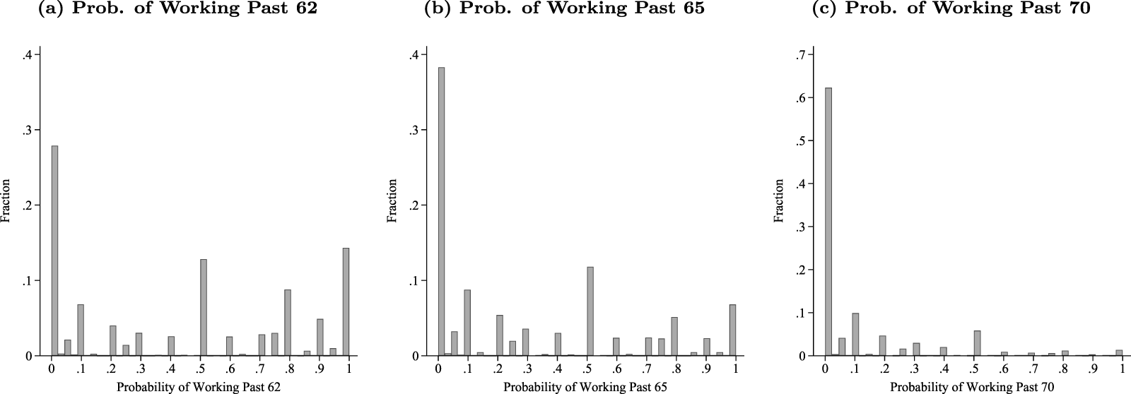

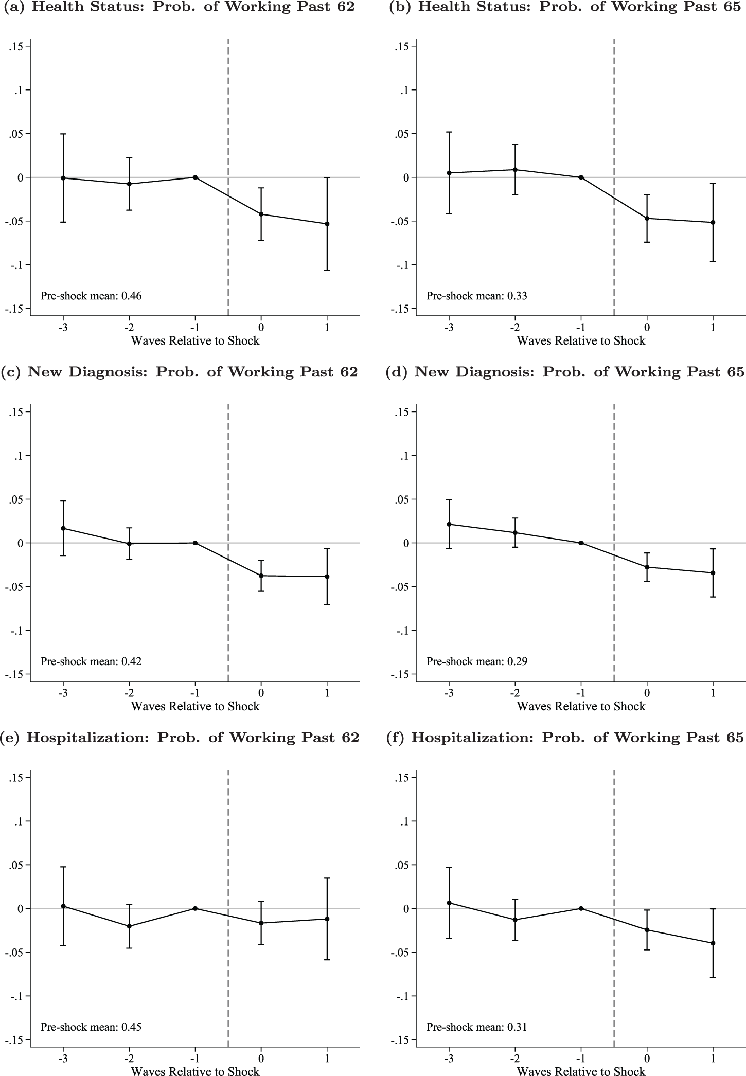

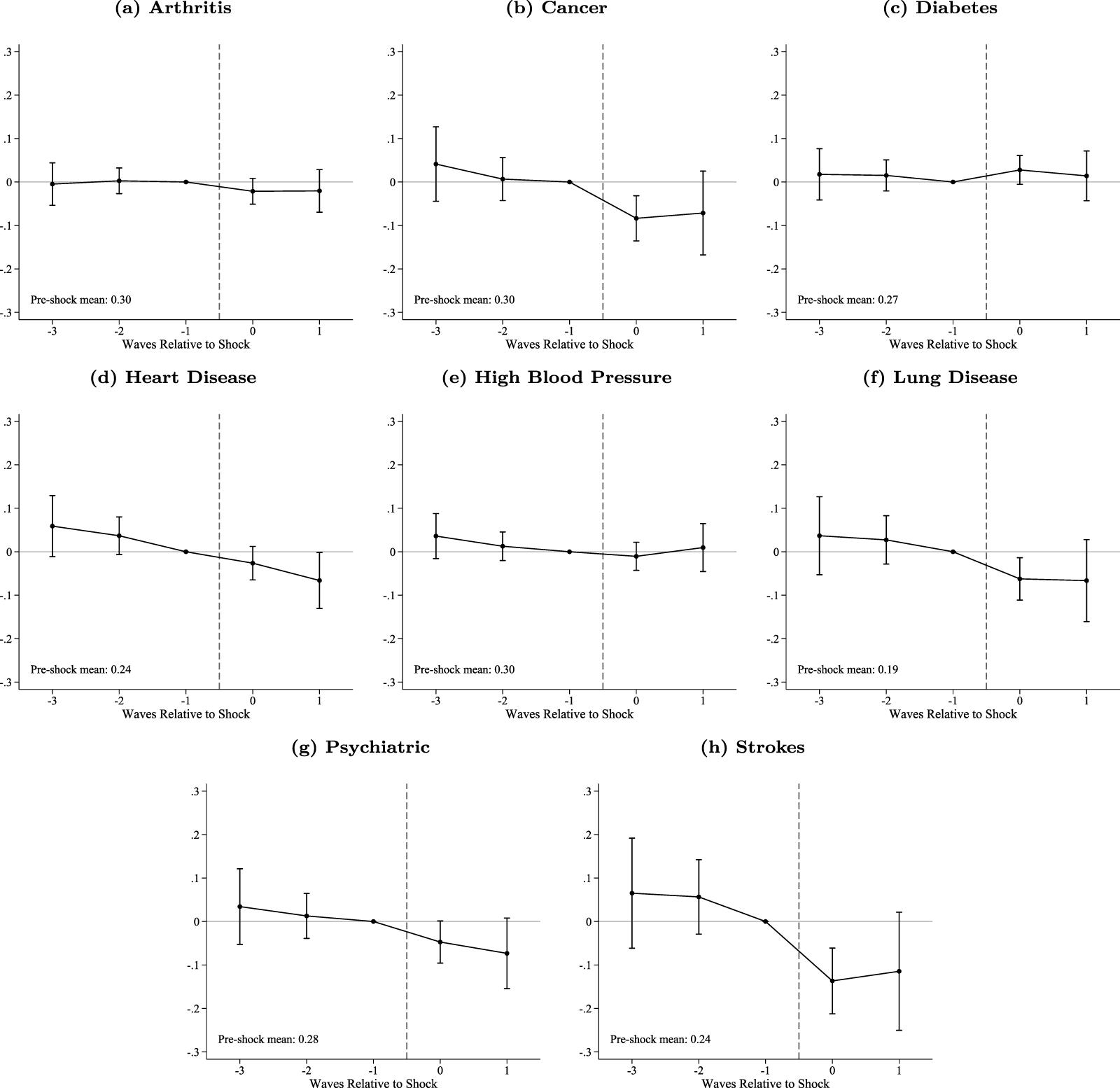


 Open access

