2.1. Equivalent back-pressure $\bar {\bar {p}}$ for over-expansion flow

Previous work (see Wang et al. Reference Wang, Xue and Cheng2018) suggests that MEP is helpful for understanding the asymmetry of shock wave interactions induced by separation. The MEP method predicts shock wave interactions by identifying the configuration that minimises entropy production among the multiple patterns satisfying the same flow conditions. The key to predicting asymmetry in over-expansion flow using MEP lies in establishing the relationship between the geometric configuration of shock wave interaction and flow conditions.

Over-expansion flow is sensitive to downstream pressure, which plays a crucial role in shock–shock interaction. The influence of downstream pressure on the flow configuration can be described by an equivalent back-pressure $\bar {\bar {p}}$ (see Wang et al. Reference Wang, Xue and Cheng2018), defined as the average pressure near the shock wave based on the mass flow rate. For a single curved shock, as shown in figure 6(a), $\bar {\bar {p}}$ is expressed as

(2.1) \begin{equation} \bar {\bar {p}} = \frac {\int \rho v p \, {\mathrm d}L'}{\int \rho v \, {\mathrm d}L'}, \end{equation}

where $\rho$ , $v$ and $p$ represent the local density, the velocity normal to the shock, and the pressure behind the shock wave $L$ , respectively, and $L'$ is a line close to shock $L$ . For RR in an over-expansion flow, as shown in figure 6(b), the equivalent pressure $\bar {\bar {p}}_{\textit{RR}}$ behind the leading shock waves can be written as

(2.2) \begin{equation} \bar {\bar {p}}_{\textit{RR}} = \frac {\int \rho _1 v_1 p_1 \, {\mathrm d}L_1 + \int \rho _2 v_2 p_2 \, {\mathrm d}L_2}{\int \rho _1 v_1 \, {\mathrm d}L_1 + \int \rho _2 v_2 \, {\mathrm d}L_2}, \end{equation}

where subscripts 1 and 2 denote the separation shocks induced from the top and bottom, respectively. Because the total mass flow rate passing through the leading shock waves is equal to that passing through the throat, and assuming that the throat flow is sonic (see Jaunet & Lehnasch Reference Jaunet and Lehnasch2025), (2.2) can be derived as

Figure 6.

Schematic illustrations of shock waves: (a) a curved shock, (b) shock interaction for over-expansion flow, and (c) definitions of flow conditions.

(2.3) \begin{equation} \bar {\bar {p}}_{\textit{RR}} = \frac {\int \rho _1 M_1 \sqrt {T_1}\, p_1 \sin (\beta _1 - \alpha _1) \, {\mathrm d}L_1 + \int \rho _2 M_2 \sqrt {T_2}\, p_2 \sin (\beta _2 - \alpha _2) \, {\mathrm d}L_2}{\rho _{\textit{th}} \sqrt {T_{\textit{th}}}\, L_{\textit{th}}}, \end{equation}

where the subscript th denotes the flow condition at the throat position, with $L_{\textit{th}}$ the throat height, and $\beta$ and $\alpha$ representing the local shock angle and flow deflection angle, respectively. To connect the shock wave configuration with flow conditions, (2.3) can be rewritten as

(2.4) \begin{equation} \begin{aligned} \bar {\bar {p}}_{\textit{RR}} = & \frac {1}{L_{\textit{th}}} \int \left ( \frac {\rho _1}{\rho _{i1}} \frac {\rho _{i1}}{\rho _{\textit{th}}} \frac {\sqrt {T_1}}{\sqrt {T_{i1}}} \frac {\sqrt {T_{i1}}}{\sqrt {T_{\textit{th}}}} p_1 M_1 \sin (\beta _1 - \alpha _1) \, {\mathrm d}L_1 \right ) \\ & {}+ \frac {1}{L_{\textit{th}}} \int \left ( \frac {\rho _2}{\rho _{i2}} \frac {\rho _{i2}}{\rho _{\textit{th}}} \frac {\sqrt {T_2}}{\sqrt {T_{i2}}} \frac {\sqrt {T_{i2}}}{\sqrt {T_{\textit{th}}}} p_2 M_2 \sin (\beta _2 - \alpha _2) \, {\mathrm d}L_2 \right ). \end{aligned} \end{equation}

Here, the subscript $i$ denotes the flow condition ahead of incident shock wave, and the aforementioned fractions can be expressed as the following functions:

(2.5) \begin{align} \frac {\rho _i}{\rho _{\textit{th}}} &= f_\rho (M_i) = \frac {\left (1 + \dfrac {\gamma - 1}{2}\right )^{\tfrac{1}{(\gamma - 1)}}}{\left (1 + \dfrac {\gamma - 1}{2} M_i^2\right )^{\tfrac{1}{(\gamma - 1)}}},\\[-7pt]\nonumber\end{align}

(2.6) \begin{align} \frac {\sqrt {T_i}}{\sqrt {T_{\textit{th}}}}& = f_T(M_i) = \sqrt {\frac {1 + \dfrac {\gamma - 1}{2}}{1 + \dfrac {\gamma - 1}{2} M_i^2}},\\[-7pt]\nonumber\end{align}

(2.7) \begin{align} \frac {p}{p_i} & = g_p(M_i, \beta ) = \frac {2\gamma }{\gamma + 1} M_i^2 \sin ^2 \beta - \frac {\gamma - 1}{\gamma + 1},\\[-7pt]\nonumber\end{align}

(2.8) \begin{align} \frac {\rho }{\rho _i} & = g_\rho (M_i, \beta ) = \frac {(\gamma + 1) M_i^2 \sin ^2 \beta }{2 + (\gamma - 1) M_i^2 \sin ^2 \beta },\\[-7pt]\nonumber \end{align}

(2.9) \begin{align} \frac {\sqrt {T}}{\sqrt {T_i}} &= g_T(M_i, \beta ) = \sqrt {\frac {(1 - \gamma + 2\gamma M_i^2 \sin ^2 \beta )\left [2 + (\gamma - 1) M_i^2 \sin ^2 \beta \right ]}{(\gamma + 1) M_i \sin \beta }},\\[-7pt]\nonumber\end{align}

(2.10) \begin{align} M & = g_M(M_i, \beta ) = \sqrt {\frac {2 + (\gamma - 1) M_i^2 \sin ^2 \beta }{(2\gamma M_i^2 \sin ^2 \beta - \gamma + 1) \sin ^2(\beta - \alpha )}} .\end{align}

Therefore, all the fractions can be treated as functions of $M_i$ and $\beta$ . According to the FIT method, $p / p_i$ can be obtained using (1.1), thus $\beta$ is also a function of $M_i$ , expressed as

(2.11) \begin{equation} \beta = f_\beta (M_i) = \sin ^{-1} \left ( \sqrt {\frac {1}{M_i^2} + (\gamma + 1)\, F(\bar {x})\, \sqrt {\frac {C_{f0}}{8\left(M_i^2 - 1\right)^{0.5}}}} \right ). \end{equation}

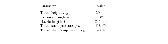
According to the conditions given in table 1, the Reynolds number Re at the throat is approximately $6.39\times {10^5}$ , and the Reynolds number increases monotonically along the flow direction. If the flow expands completely, then Re at the exit is approximately ${9.6}\times {10^5}$ . Therefore, the flow is turbulent and $ F(\bar {x})_{\textit{turp}} \approx 6$ . The $C_{f0}$ value is related to $M_i$ and Re, with detailed derivation given by Matheis & Hickel (Reference Matheis and Hickel2015). Equations (2.5)–(2.11) indicate that $\bar {\bar {p}}_{\textit{RR}}$ can be considered as a function of $M_i$ , which is expressed by

(2.12) \begin{equation} \bar {\bar {p}}_{\textit{RR}} = h_{p_{\textit{RR}}}(M_{i1}, M_{i2}). \end{equation}

The expanded duct forms an expansion region ahead of the shock waves, resulting in non-uniform flow parameters and curved shock waves, as shown in figure 6(c). The local Mach numbers $M_{i1}$ and $M_{i2}$ ahead of the leading shock waves are determined by the nozzle contour, which are related to positions $x_{1}$ and $x_{2}$ . Consequently, the relationship among the equivalent pressure $\bar {\bar {p}}_{\textit{RR}}$ and the separation positions on top ( $x_1$ ) and bottom ( $x_2$ ) is established (with $x=0$ defined at the position of the throat):

(2.13) \begin{equation} \bar {\bar {p}}_{\textit{RR}} = h_{p_{\textit{RR}}}(x_1, x_2). \end{equation}

Table 1.

Key parameters of the nozzle.

A flow field of MR is depicted schematically in figure 10(b) below. Since a Mach stem $L_5$ takes part in the shock configuration, the function $\bar {\bar {p}}_{MR}$ should become

(2.14) \begin{equation} \bar {\bar {p}}_{\textit{MR}} = \frac {\int \rho _1 v_1 p_1 \, {\mathrm d}L_1 + \int \rho _2 v_2 p_2 \, {\mathrm d}L_2+\int \rho _5 v_5 p_5 \, {\mathrm d}L_5}{\int \rho _1 v_1 \, {\mathrm d}L_1 + \int \rho _2 v_2 \, {\mathrm d}L_2 +\int \rho _5 v_5 \, {\mathrm d}L_5}, \end{equation}

where the subscript 5 denotes the flow condition behind the Mach stem. The Mach stem is a strongly curved shock, the pressure change of which is close to that of a normal shock (see Bai & Wu Reference Bai and Wu2017), hence it may be treated as a section of a normal shock (see Wang et al. Reference Wang, Xue and Cheng2018) in the current study. Here, a new parameter $l$ , the height of the Mach stem, is added to the expression for $\bar {\bar {p}}_{\textit{MR}}$ :

(2.15) \begin{equation} \bar {\bar {p}}_{\textit{MR}} = h_{p_{\textit{MR}}}(x_1, x_2, l). \end{equation}

Additionally, there is a maximum value for the flow deflection angle $\alpha$ , beyond which the reflected shock becomes a normal shock, as shown in figure 7(a). As the shock separation point moves upstream, the pressure–deflection polar line of the incident shock changes from $IS_1$ to $IS_3$ , while the reflected shock changes from $\textit{RS}_1$ to $\textit{RS}_3$ , resulting in a decrease in the maximum flow deflection angle. Consequently, a critical position $x^*$ exists, and for $x \lt x^*$ , the reflected shock does not exist, as shown in figure 7(b). For better understanding, several key parameters of the nozzle contour shown in figure 6(b) are provided in table 1, and the corresponding relation curves based on $\bar {\bar {p}}$ are illustrated in figure 8, where $x^*$ corresponds to ${\bar {\bar {p}}}/{p_{\textit{th}}} = 0.73$ .

Figure 7.

Diagrams illustrating the maximum of $\bar {\bar {p}}$ : (a) pressure–deflection polar lines illustrating the maximum deflection angle $\alpha$ of the separated shock waves; (b) comparison between the maximum separation shock angle $\beta _{max}$ and the separation shock angle based on FIT.

Figure 8.

Diagrams illustrating solution domains of separation positions and shock angles: (a) relation among $x_1$ , $x_2$ and $\bar {\bar {p}}$ ; (b) relation among $\beta _1$ , $\beta _2$ and $\bar {\bar {p}}$ .

Figure 9.

Possible configurations based on different solution domains: (a) symmetric RR in S, (b) RR in B $_2$ , (c) RR in B $_1$ , (d) asymmetric RR in domain I, (e) asymmetric RR in domain II, ( f) symmetric MR in S, (g) MR in B $_2$ , (h) MR in B $_1$ , (i) asymmetric MR in domain III, (j) asymmetric MR in domain IV.

As shown in figure 8(a), the separation positions on the top and bottom walls ( $x_1$ and $x_2$ ) at a constant $\bar {\bar {p}}$ lie on a curve that is symmetrically distributed around the diagonal S, with the curves moving upstream as $\bar {\bar {p}}$ increases. Similarly, the separation shock angles near the interaction point ( $\beta _1$ and $\beta _2$ ), as shown in figure 8(b), also form symmetric curves along S, and gradually increase with the rise in $\bar {\bar {p}}$ . The possible flow patterns are illustrated in figure 9 according to the solution domain. Figure 9(a) shows a symmetric interaction, which corresponds to solutions where ( $x_1$ , $x_2$ ) or ( $\beta _1$ , $\beta _2$ ) meet at S, as shown in figure 8. Figure 8 shows boundaries B $_1$ and B $_2$ , where the leading shock waves degenerate into one oblique shock and one reflected shock, as shown in figures 9(b) and 9(c). Line C is an important critical line for RR and MR, marked in red in figure 8. When RR-to-MR transition occurs, the Mach stem appears and grows gradually (see Shimshi et al. Reference Shimshi, Ben-Dor and Levy2009). Here, to clearly show the boundary between RR and MR, the equivalent back-pressure $\bar {\bar {p}}$ for MR is calculated with $l=0$ ; the effect of $l$ will be discussed in detail in the next subsection. Lines C and S divide the overall solution space into four regions, denoted as domains I to IV, which correspond to multiple configurations shown in figure 9(d–j). The critical line C will be discussed in the following paragraphs.

Figure 10.

Schematic illustrations of shock reflections in over-expansion flow: (a) RR, (b) MR.

The RR configuration, as shown in figure 10(a), consists of two incident shocks, denoted by $I_1$ on the top wall and $I_2$ on the bottom wall, and double asymmetrical reflected shocks, denoted by $R_1$ and $R_2$ . An overall RR boundary condition requires that all the incident and reflected shocks meet at a single node, denoted by $O$ . The overall MR, as shown in figure 10(b), is more complicated than the overall RR, where a very strong curved shock, known as the Mach stem, is added to the configuration. As a result, the incident shocks and reflected shocks cannot meet at a single node, and are instead replaced by two endpoints of the Mach stem, denoted by $O_1$ and $O_2$ , respectively.

The possible solutions for asymmetric shock reflection are described by pressure–deflection polar lines, as illustrated in figure 11(a). Here, $I_1$ and $I_2$ are the incident shock polar lines on the top and bottom walls, respectively, along which the pressures satisfy the oblique shock wave equations (see Li et al. Reference Li, Chpoun and Ben-Dor1999). In a uniform flow, the possible solutions for the reflected shock waves (denoted as $R_1$ and $R_2A$ to $R_2E$ ) are indicated by the intersections (denoted as points $A$ to $E$ ). Two classical criteria (see von Neumann Reference von Neumann1943, Reference von Neumann1945) – the von Neumann criterion and the detachment criterion, denoted as $\alpha ^{vN}$ and $\alpha ^D$ respectively – divide the solution domain into three portions: RR exists in flows where $\alpha _2\lt \alpha ^{vN}$ , such as $R_2A$ ; MR exists in flows where $\alpha _2\gt \alpha ^D$ , such as $R_2E$ ; and both RR and MR could exist in flows where $\alpha ^{vN} \leqslant \alpha _2 \leqslant \alpha ^D$ , such as $R_2C$ . In addition, the minimum valid Mach number for the von Neumann criterion is $M \approx 2.2$ .

Figure 11.

Pressure–deflection polar lines illustrating various possible solutions: (a) interaction in a uniform flow, (b) symmetric interaction in a non-uniform flow, and (c) asymmetric interaction in a non-uniform flow.

In the current study, the expansion flow is non-uniform as shown in figure 10, meaning that the Mach number $M_i$ and pressure $p_i$ ahead of the interaction point may change as the interaction point moves. Therefore, we employ $p/p_{\textit{th}}$ to measure the pressure rise when the flow passes through a shock wave. The pressure–deflection polar lines, which correspond to the solutions from $a$ to $f$ given in figure 8, are illustrated in figures 11(b) and 11(c). For the symmetric configuration, the solutions moving from $a$ to $c$ are shown in figure 11(b), where the double polar lines of reflected shocks move away from each other, and point $b$ represents the detachment criterion where reflected lines are tangent. Similarly, in asymmetric interaction, the solutions moving from $d$ to $f$ also experience a detachment criterion at point $e$ , as shown in figure 11(c). Accordingly, all the detachment criterion points form a critical line C, marked in red in figure 8, and the RR configurations shown in figure 9(a–e) each correspond to an MR mode, as shown in figure 9( f–j), respectively.

2.2. Prediction of flow pattern based on MEP

In § 2.1, ten possible configurations of the over-expansion flow are discussed, while the actual flow with the highest likelihood requires a prediction method, which is proposed based on MEP in this subsection. The entropy production (denoted by $\dot {S}$ ) of flow passing through a shock wave, as shown in figure 6(a), can be expressed as follows (see Li & Ben-Dor Reference Li and Ben-Dor1996a , Reference Li and Ben-Dor1997):

(2.16) \begin{equation} \dot {S} = \int \rho v\, \Delta s \, {\mathrm d}L, \end{equation}

where $\Delta s$ is the entropy change across the shock wave $L$ , given by

(2.17) \begin{equation} \Delta s = -C_v (\gamma - 1) \ln \left ( \frac {p_0}{p_{0i}} \right ). \end{equation}

Here, $ p_{0i}$ and $ p_0$ represent the total pressures ahead of and behind the shock wave, respectively. For the RR configuration shown in figure 6(b), the total entropy production $\dot {S}_{\textit{RR}}$ generated by incident and reflected shocks can be written as

(2.18) \begin{equation} \dot {S}_{\textit{RR}} = \int \rho _1 v_1\, \Delta s_1 \, {\mathrm d}L_1 + \int \rho _2 v_2\, \Delta s_2 \, {\mathrm d}L_2 + \int \rho _3 v_3\, \Delta s_3 \, {\mathrm d}L_3 + \int \rho _4 v_4\, \Delta s_4 \, {\mathrm d}L_4 \end{equation}

for computational convenience. Then $\dot {S}_{\textit{RR}}$ is non-dimensionalised as $\ddot {S}_{\textit{RR}}$ :

(2.19) \begin{equation} \ddot {S}_{\textit{RR}} = \frac {\dot {S}}{C_v (\gamma - 1) \rho _{\textit{th}} L_{\textit{th}} \sqrt {\gamma R T_{\textit{th}}}}. \end{equation}

Then (2.19) is derived as

(2.20) \begin{equation} \ddot {S}_{\textit{RR}} = -\frac {1}{\rho _{\textit{th}} L_{\textit{th}} \sqrt {T_{\textit{th}}}} \sum _{n=1}^4 \int \rho _n M_n \sqrt {T_n} \ln \left ( \frac {p_{0n}}{p_{0in}} \right ) \sin (\beta _n - \alpha _n) \, {\mathrm d}L_n, \end{equation}

where $n = 1$ and $n = 2$ represent the double incident shocks, and $n = 3$ and $n = 4$ represent the double reflected shocks. The fraction ${p_0}/{p_{0i}}$ can be written as a function of $M_i$ and $\beta$ :

(2.21) \begin{equation} \frac {p_0}{p_{0i}} = g_{p_0}(M_i, \beta ) = \big [g_p(M_i, \beta )\big ]^{\tfrac{-1}{(\gamma -1)}} \big [g_\rho (M_i, \beta )\big ]^{\tfrac {\gamma }{(\gamma -1)}}. \end{equation}

Reflected shocks are determined by incident shocks, and all the variables can be derived from the functions of $ f$ and $ g$ given in (2.5)–(2.11) and (2.21). Thus $ \ddot {S}_{\textit{RR}}$ is also a function of $ (M_i, \beta )$ . Since the distribution of $ (M_i, \beta )$ depends on $ (x_1, x_2)$ , similar to the derivation of $ \bar {\bar {p}}_{\textit{RR}}$ in (2.13), $ \ddot {S}_{\textit{RR}}$ can be expressed as

(2.22) \begin{equation} \ddot {S}_{\textit{RR}} = {f_{S}}_{\textit{RR}}(x_1, x_2). \end{equation}

Figure 12.

Diagram illustrating entropy production distribution: (a) based on $(x_1,x_2)$ , and (b) based on $(\beta _1,\beta_2)$ .

In § 2.1, the relationship between $ x_1$ , $ x_2$ and $ \bar {\bar {p}}$ has been discussed, and there is a series of combinations of $ x_1$ and $ x_2$ at a constant $ \bar {\bar {p}}$ , as shown in figure 8. It has been proved above that any one of $ x_1$ , $ x_2$ and $ \bar {\bar {p}}$ can be obtained from the other two (see 2.13). Hence, inserting $x_2 = h_{{p_{\textit{RR}}}}^{-1}(x_1, \bar {\bar {p}})$ into (2.22), the total entropy production factor also can be written as

(2.23) \begin{equation} \ddot {S}_{\textit{RR}} = {f_{S}}_{\textit{RR}}(x_1, \bar {\bar {p}}). \end{equation}

For given downstream equivalent back-pressure $\bar {\bar {p}}_{\textit{RR}}$ , $ \ddot {S}_{\textit{RR}}$ is related to $ x_1$ (or $ x_2$ ). Therefore, according to MEP, the configuration is determined by the local minima of $ \ddot {S}_{\textit{RR}}$ . For better understanding, figure 12(a) provides an example to illustrate the relation among $ \ddot {S}_{\textit{RR}}$ and separation positions on top ( $ x_1$ ) and bottom ( $ x_2$ ), when ${\bar {\bar {p}}}/{p_{\textit{th}}} = 0.35$ . Two points satisfy the minima conditions:

(2.24) \begin{equation} \left . \begin{array}{c} \dfrac {\partial {f_{S}}_{\textit{RR}}}{\partial x_1} = 0, \\[8pt] \dfrac {\partial ^2 {f_{S}}_{\textit{RR}}}{\partial x_1^2} \geqslant 0. \end{array} \right \} \end{equation}

This results in ${x_1}/{L_{\textit{th}}} = 6.7$ and ${x_2}/{L_{\textit{th}}} = 7.4$ , or ${x_1}/{L_{\textit{th}}} = 7.4$ and ${x_2}/{L_{\textit{th}}} = 6.7$ , which correspond to two asymmetrical RR configurations that fulfil the MEP. The corresponding relationship among $\ddot {S}_{\textit{RR}}$ and the separation shock angle on top ( $\beta _1$ ) and bottom ( $\beta _2$ ) is shown in figure 12(b). These two asymmetric structures are essentially the same, with the difference being in the direction of asymmetry.

In MR, the factor $\dot {S}_{\textit{MR}}$ of total entropy production should contain the contribution of $L_5$ and results in

(2.25) \begin{equation} \dot {S}_{\textit{MR}} = \sum _{i=1}^5 \int \rho _i v_i\, \Delta s_i \, {\mathrm d}L_i. \end{equation}

Here, the Mach stem is treated as a normal shock, and the contribution of total entropy production is affected by its length $l$ . Thus $\ddot {S}_{\textit{MR}}$ can be expressed as

(2.26) \begin{equation} \ddot {S}_{\textit{MR}} = {f_{S}}_{\textit{MR}}(x_1, x_2,l). \end{equation}

Similarly, inserting $x_2 = h_{{p_{\textit{MR}}}}^{-1}(x_1,l, \bar {\bar {p}})$ into (2.26), the total entropy production factor also can be written as

(2.27) \begin{equation} \ddot {S}_{\textit{MR}} = {f_{S}}_{\textit{MR}}(x_1,l, \bar {\bar {p}}). \end{equation}

The relations among $\ddot {S}_{\textit{MR}}$ , $\bar {\bar {p}}_{\textit{MR}}$ , $l$ , $x_1$ and $x_2$ are depicted schematically in figure 13. When ${\bar {\bar {p}}}/{p_{\textit{th}}} = 0.5$ , changes in $l$ lead to different solutions for MEP. There exists a critical length $l^*$ (with $ {l^*}/{L_{\textit{th}}} \approx 0.25 $ ), such that when $l \lt l^*$ , the entropy production curve exhibits two minimum points, as shown in figure 14(a), corresponding to asymmetric MR, and when $l \geqslant l^*$ , the entropy production curve has only one minimum point, as shown in figure 14(b), corresponding to symmetric MR. The value of $l^*$ depends on $\bar {\bar {p}}$ and increases as $\bar {\bar {p}}$ increases.

Figure 13.

Diagram illustrating entropy production distribution based on $x_1$ , $x_2$ and $l$ at ${\bar {\bar {p}}}/{p_{\textit{th}}} = 0.5$ .

Figure 14.

Diagram illustrating entropy production distribution at ${\bar {\bar {p}}}/{p_{\textit{th}}} = 0.5$ based on $(x_1,x_2)$ with different Mach stem lengths: (a) ${l}/{L_{\textit{th}}} = 0.1$ and (b) ${l}/{L_{\textit{th}}} = 0.4$ .

Therefore, as $\bar {\bar {p}}$ changes, the flow configuration that fulfils the MEP also changes. Figure 15 shows the separation positions of the MEP structure with the change of $\bar {\bar {p}}$ . In this figure, the red solid line L $_1$ represents the criterion for the transition between RR and MR, and RR resides in the domain above L $_1$ , while MR is below L $_1$ . The purple and cyan solid lines L $_2$ and L $_3$ represent two MEP solutions for RR, suggesting that shock waves may form two asymmetric structures. The yellow and blue solid lines L $_4$ and L $_5$ represent two MEP solutions for MR when the Mach stem length $l$ is close to zero, indicating two asymmetric structures. The green solid line L $_6$ represents the MEP solution for MR when the Mach stem length exceeds $l^*$ , indicating that the shock wave interaction is more likely to be a symmetric configuration. Domains I and II are possible solutions for $0 \lt l \lt l^*$ . The black dashed line L $_7$ denotes ${\bar {\bar {p}}}/{p_{\textit{th}}} = 0.73$ , corresponding to the solution boundary, and when ${\bar {\bar {p}}}/{p_{\textit{th}}} \gt0.73$ , the reflected shock may become a normal shock. The black dash-dotted line L $_8$ represents the physical boundary of walls, and the effective separation points must exist in the region enclosed by the boundary. The black solid line L $_9$ is another boundary at ${\bar {\bar {p}}}/{p_{\textit{th}}} = 0.3$ , and when ${\bar {\bar {p}}}/{p_{\textit{th}}} \lt 0.3$ , the separation positions will move out of the expansion section. Finally, the orange solid line in the inset represents the variation of $l^*$ with the change of $\bar {\bar {p}}$ . The theoretical results are validated and analysed in the next section.

Figure 15.

Diagram illustrating the relations between $\bar {\bar {p}}$ and $(x_1, x_2)$ that fulfil the MEP.

Figure 16.

The experimental set-up: (a) physical diagrams of the model; (b) schematic diagram of the model; (c) Mach number along the central line; and (d) optical diagnostics.

3.1. Test model and apparatus

The experiments were conducted in a blow-down type wind tunnel at Nanjing University of Aeronautics and Astronautics. The test model consists of a converging–diverging nozzle, as shown in figure 16(a), with a straight duct containing a throttling device mounted downstream of the expansion section. The main dimensions of the model are indicated in figure 16(b). The divergent section has length 215 mm with expansion angles $4^\circ$ on both sides. The throat (inlet of the divergent section) has height 20 mm, while the outlet matches the straight duct height 50 mm. The convergent section is 60 mm long with inlet height 60 mm. The contraction curve follows the Witoszynski profile (see Kuz‘Min & Khazhuev Reference Kuz‘Min and Khazhuev1993), which can be represented by

(3.1) \begin{equation} y = \frac {y^*}{\sqrt {1 - \Psi }}, \quad \Psi = \frac {\big [1 - \left ({y^*}/{y_0}\right )^2\big ]\big[1 - (x/L)^2\big]^2}{\big[1 + (x/L)^2/3\big]^3}, \quad x \in [0,60]. \end{equation}

Here, $y^*$ and $y_0$ represent the half-heights at the throat and at the entrance, respectively, while $x$ denotes the axial coordinate measured from the convergent entrance, and $L$ is the convergent portion length. These parameters are specified as $y^*= 30$ , $y_0= 10$ , $L= 60$ and $x \in [0, {60}\ \textrm {mm} ]$ . The width of the model remains 50 mm. The Mach number distribution, ranging from 1 to 2.4 along the centreline of the expansion section, is shown in figure 16(c). A throttling device driven by a step motor (see Wang et al. Reference Wang, Xue and Cheng2018) was employed to guide the downstream pressure disturbance.

Six pressure transducers, labelled T $_1$ to T $_6$ , were mounted on the top and bottom walls of the expansion section, and two transducers, labelled T $_{\textrm{B}1}$ and T $_{\textrm{B}2}$ , were mounted at the end of the straight section, as shown in figure 16(b). A dedicated stagnation pressure probe was installed upstream of the converging section, aligned with the freestream flow direction to measure total pressure $ p_c$ . All transducers are Kulite XTEL-190SM, operated at rate 10 kHz using data acquisition cards with a 20 s sampling time. There are two optical glasses respectively embedded into sidewalls for the schlieren system, as shown in figure 16(d). An NAC (NAC Image Technology) Hotshot high-speed camera, which operated at frame rate 5 kHz with a 5.8 s sampling time and resolution 768 $\times$ 544 pixels, was used to capture the evolution of the shock wave configuration.

Figure 17.

Time histories of pressure during one test.

Figure 17 shows the time histories during one test. The wind tunnel starts at $ t_{w1}$ ; after the flow field is established (the total pressure $ p_c$ is stable), the schlieren camera shooting starts at $ t_{s1}$ and stops at $ t_{s2}$ ; the downstream throttling starts at $ t_{t1}$ and stops at $ t_{t2}$ ( $ t_{s1}$ is earlier than $ t_{t1}$ , and $ t_{t2}$ is earlier than $ t_{s2}$ ); and finally, the wind tunnel stops at $ t_{w2}$ . The experimental data captured from $ t_{t1}$ to $ t_{t2}$ are mainly analysed in the next subsection.

3.2. Results and discussion

The shock wave moves upstream as the NPR decreases, with the changes in wall pressure illustrated in figure 18(a). Since throttling starts at $ t_{t1} = 5.6 \, \text{s}$ , T $_{\textrm{B}1}$ and T $_{\textrm{B}2}$ , which are located on the same vertical plane near downstream throttling, increase smoothly and nearly overlap, indicating that the downstream pressure disturbance is symmetric. Although incoming flow is also symmetric, pressures acquired in the expansion section fluctuate inconsistently. Here, T $_3$ and T $_6$ are located on the same vertical plane, while T $_3$ first senses pressure fluctuation, and T $_6$ lags behind T $_3$ . Then a similar process can be seen in T $_2$ and T $_5$ , meaning that the shock wave interaction is asymmetric. The motion of separation points on top ( $ x_1$ ) and bottom ( $ x_2$ ), based on statistics from 20 000 schlieren images, is shown in figure 18(b), demonstrating that the interaction maintains an asymmetric pattern and moves upstream with NPR decreasing from 2.7 to 1.6, as shown in figure 18(c). Additionally, both RR and MR configurations are observed during this process, with the RR-to-MR transition occurring at $ t = 7.8 \ \text{s}$ , when the Mach stem appears. Figure 18(d–h) show the flow patterns of shock wave motion. As can be seen, the main flow deflects downwards, with a large separation region on top, and a local separation region on the bottom. The Mach stem is not distinct initially, as shown in figure 18( f), but at $ t = 9.4 \ \text{s}$ in figure 18(h), the Mach stem has a significant growth.

Figure 18.

Experimental characteristics of flow configuration: (a) dynamic wall pressures, (b) separation positions, (c) NPR, and (d–h) schlieren images at different times.

The separation shock strength near the boundary layer can be analysed using FIT. For an expansion flow, the local Mach number varies with position, so the separation strength predicted by the FIT is influenced by the Mach number ahead of the shock wave (see Aghababaie & Theunissen Reference Aghababaie and Theunissen2015). In the current study, both separation shock waves on the top and bottom walls, based on 20 000 images, are statistically analysed and summarised in figure 19(a), where the black solid lines are theoretical results of FIT, the red dots correspond to the experimental values of the bottom separation shock angles, and the green dots represent the top separation shock angles (where clockwise is positive). As can be seen, the experimental results on both the top and bottom agree well with FIT. It should be noted that the theoretical lines are symmetric about the centreline, which does not imply that the flow patterns in the experiment are symmetric. Therefore, FIT cannot explain the asymmetry of shock wave interactions. Figure 19(b) illustrates a comparison between experimental results and MEP, where the definitions of the theoretical lines have been described by figure 15. As shown in figure 19(b), the separation points $(x_1, x_2)$ are distributed around L $_2$ and L $_4$ , which respectively represent asymmetric RR and asymmetric MR. As NPR decreases, the flow pattern transitions from RR to MR, with the asymmetric structure being the dominant phenomenon. Here, L $_4$ is the line where the Mach stem length is close to zero, while the actual Mach stem grows with the upstream motion of the shock wave. The region between L $_4$ and L $_6$ represents the possible MR pattern when $0 \lt l \lt l^*$ . Therefore, during the MR stage (the domain below L $_1$ ), the experimental data initially agree well with L $_4$ , and the locations of points tend to move closer to the centreline as the Mach stem gradually grows. Since the Mach stem length $l$ is always shorter than $l^*$ , the flow pattern maintains an asymmetric configuration over a wide range, and very few symmetric points are found in the area close to L $_7$ , which is the boundary ${\bar {\bar {p}}}/{p_{\textit{th}}} = 0.73$ .

Figure 19.

Comparison between experimental results and theoretical values: (a) the separation strengths based on FIT; (b) the separation positions based on MEP.

To capture the transition between symmetric MR (SMR) and asymmetric MR (AMR), a secondary test was conducted. As shown in figure 20(a), T $_1$ and T $_4$ , which are located on the same vertical plane near the throat, recorded the key time histories of wall pressures with NPR increasing from 1 to 1.7, shown in figure 20(b), during which typical schlieren images are shown in figure 20(c–h). When $t \lt t_1$ (4.3 s) and $\text{NPR} \lt 1.1$ , corresponding to ${\bar {\bar {p}}}/{p_{\textit{th}}} \gt 0.73$ , the MR is not shaped, and the shock wave is mostly like a normal shock, as shown in figure 20(c). At $t_2$ = 4.5 s, ${\bar {\bar {p}}}/{p_{\textit{th}}}\approx 0.72$ , MR can be identified, and it is a symmetric pattern, as shown in figure 20(d). An interesting phenomenon occurs at approximately 4.7 s, where ${\bar {\bar {p}}}/{p_{\textit{th}}}$ at both $t_3= 4.7$ s and $t_4= 4.75$ s is approximately 0.71, with a sudden reduction in Mach stem length ( ${l}/{L_{\textit{th}}}$ changes from 0.6 to 0.19), while the former one is SMR shown in figure 20(e), and the latter is AMR shown in figure 20( f), indicating that the SMR-to-AMR transition is closely related to the Mach stem. At $t_5= 5.0$ s and $t_6= 5.2$ s, the AMR structure gradually moves downstream as shown in figures 20(g) and 20(h).

Figure 20.

Experimental characteristics of flow configuration in secondary test: (a) the pressure changes recorded by $\text{T}_1$ and $\text{T}_4$ ; (b) the NPR; and (c–h) schlieren images at different times.

The entropy production curves at ${\bar {\bar {p}}}/{p_{\textit{th}}} = 0.71$ with two different Mach stem lengths are illustrated in figure 21(a). Apparently, there is only one MEP solution with ${l}/{L_{\textit{th}}} = 0.6$ , which represents an SMR pattern where $x_1 = x_2$ , while there are two solutions with ${l}/{L_{\textit{th}}} = 0.19$ , which represents an AMR pattern where $x_1 \neq x_2$ , demonstrating good agreement between the experiment and MEP. The experimental results of Mach stem lengths containing both SMR and AMR are summarised in figure 21(b), where the solid line is the theoretical prediction of $l^*$ based on MEP. As can be seen, SMR resides in the domain of relatively high ${\bar {\bar {p}}}/{p_{\textit{th}}}$ , and $l$ is mostly larger than $l^*$ . With the decrease of ${\bar {\bar {p}}}/{p_{\textit{th}}}$ , $l^*$ also reduces smoothly, and $l$ has a distinct reduction that is much lower than $l^*$ , accompanying the SMR-to-AMR transition. This process demonstrates that the shock wave interaction in such an expansion duct strives to find a pattern with low total pressure loss, and the asymmetric interaction is a way by which flow can reach a more efficient thermodynamic balance, where the entropy production tends to be minimised.

Figure 21.

Diagrams illustrating the MEP solutions for MR: (a) at ${\bar {\bar {p}}}/{p_{\textit{th}}} = 0.71$ with different Mach stem lengths; (b) comparison between $l^*$ and Mach stem length in secondary experiment as $\bar {\bar {p}}$ decreases.

Figure 22.

Flow patterns based on schlieren images captured by Verma & Manisankar (Reference Verma and Manisankar2014): (a) SMR, (b) AMR, (c) the MEP solution corresponding to SMR, and (d) the MEP solutions corresponding to AMR.

Figure 23.

Flow patterns based on schlieren images captured by Bourgoing & Reijasse (Reference Bourgoing and Reijasse2005): (a) SMR, (b) AMR, (c) the MEP solution corresponding to SMR, and (d) the MEP solutions corresponding to AMR.

The results discussed above prove the effectiveness of applying MEP to the asymmetry of over-expansion flow. Further analyses on other works are conducted to confirm the universality of the MEP method. Verma & Manisankar (Reference Verma and Manisankar2014) experimentally investigated the expansion flows in supersonic nozzles, and both SMR and AMR were observed by schlieren images, as shown in figures 22(a) and 22(b), respectively. Based on the analytical method proposed in the current work, the theoretical curves corresponding to figures 22(a) and 22(b) are illustrated in figures 22(c) and 22(d), respectively, where the relationships among $\ddot {S}$ , $x_1$ and $x_2$ are clearly described. In the case $\text{NPR} = 1.4$ , the theoretical curves indicate a single MEP solution shown in figure 22(c), demonstrating an SMR pattern and that $x_1/{L_{\textit{th}}} = x_2/{L_{\textit{th}}} = 1.2$ , which agrees well with the SMR in the schlieren image and both separation positions of $1.2L_{\textit{th}}$ shown in figure 22(a). Similarly, good agreement can be found between figures 22(b) and 22(d), where two MEP solutions indicate AMR patterns with $x_1 \neq x_2$ . It is noted that the Mach stem of AMR was much shorter than that of SMR, which fulfils the rule predicted by MEP. Another experimental study was conducted by Bourgoing & Reijasse (Reference Bourgoing and Reijasse2005), who also observed both SMR and AMR, as shown in figures 23(a) and 23(b), respectively. Accordingly, figures 23(c) and 23(d) give the corresponding analyses, which also show good agreement between experiments and MEP solutions. Therefore, the asymmetry of over-expansion flow in other works can also be well explained. The FIT is a classical theory for analysing supersonic separation flow, while it cannot explain the asymmetry of over-expansion flow. The MEP overcomes the limitation of FIT, and the combined MEP-FIT framework provides a more comprehensive description of shock structures and separation behaviours in over-expansion flows. Consequently, it can be concluded that the MEP has provided excellent supplements and extensions to the classical FIT method.