2.1 Numerical method

Throughout this paper, instantaneous, mean and fluctuating velocity fields are denoted as $u_{i}^{\ast }$ , $U_{i}$ and $u_{i}$ respectively (where $i=1,2,3$ ), and the corresponding variables for pressure and temperature are $p^{\ast }$ , $P$ , $p$ and $T^{\ast }$ , $\langle T\rangle$ , $T$ respectively. Close to the cylinder, the velocity vector is decomposed into radial, azimuthal and spanwise components which are represented with the subscripts $r,\unicode[STIX]{x1D703}$ and $z$ respectively. Following the above notation, the instantaneous velocities are represented as $u_{r}^{\ast }$ , $u_{\unicode[STIX]{x1D703}}^{\ast }$ , $u_{z}^{\ast }$ , the mean velocities as $U_{r}$ , $U_{\unicode[STIX]{x1D703}}$ , $U_{z}$ and the fluctuating components as $u_{r}$ , $u_{\unicode[STIX]{x1D703}}$ and $u_{z}$ . The continuity, momentum and temperature conservation equations are written for an incompressible flow as

(2.1) $$\begin{eqnarray}\displaystyle & \displaystyle \frac{\unicode[STIX]{x2202}u_{i}^{\ast }}{\unicode[STIX]{x2202}x_{i}}=0, & \displaystyle\end{eqnarray}$$

(2.2) $$\begin{eqnarray}\displaystyle & \displaystyle \frac{\unicode[STIX]{x2202}u_{i}^{\ast }}{\unicode[STIX]{x2202}t}+u_{j}^{\ast }\frac{\unicode[STIX]{x2202}u_{i}^{\ast }}{\unicode[STIX]{x2202}x_{j}}=-\frac{1}{\unicode[STIX]{x1D70C}}\frac{\unicode[STIX]{x2202}p^{\ast }}{\unicode[STIX]{x2202}x_{i}}+\unicode[STIX]{x1D708}\frac{\unicode[STIX]{x2202}^{2}u_{i}^{\ast }}{\unicode[STIX]{x2202}x_{j}\unicode[STIX]{x2202}x_{j}}, & \displaystyle\end{eqnarray}$$

(2.3) $$\begin{eqnarray}\displaystyle & \displaystyle \frac{\unicode[STIX]{x2202}T^{\ast }}{\unicode[STIX]{x2202}t}+u_{j}^{\ast }\frac{\unicode[STIX]{x2202}T^{\ast }}{\unicode[STIX]{x2202}x_{j}}=\unicode[STIX]{x1D6FC}\frac{\unicode[STIX]{x2202}^{2}T^{\ast }}{\unicode[STIX]{x2202}x_{j}\unicode[STIX]{x2202}x_{j}}, & \displaystyle\end{eqnarray}$$

where $\unicode[STIX]{x1D70C}$ , $\unicode[STIX]{x1D708}$ and $\unicode[STIX]{x1D6FC}$ are the density, kinematic viscosity and thermal diffusivity respectively.

These governing equations are solved using an in-house parallel code named ‘Pantarhei’. It is an unstructured finite volume solver in collocated variable arrangement. The convective and diffusion terms are discretised by a second-order central differencing scheme, while the transient term is discretised by a second-order backward scheme. The code is parallelised using the PETSc libraries (Balay et al. Reference Balay, Abhyankar, Adams, Brown, Brune, Buschelman, Eijkhout, Gropp, Kaushik and Knepley2014). Details of the solver have been reported in previous studies (Paul Reference Paul2017; Paul et al. Reference Paul, Papadakis and Vassilicos2017; Paul, Papadakis & Vassilicos Reference Paul, Papadakis and Vassilicos2018), and are not repeated here.

2.2 Numerical challenges

This study presents DNS results of heat transfer from a circular cylinder immersed in the turbulent wake generated by a single square grid-element. A study of this kind is numerically challenging due to several factors. Firstly, the surfaces of the grid-element require fine resolution to capture the correct dynamics of the turbulent flow it generates, while the flow close to the surface of the cylinder also has to be resolved well in order to predict the correct heat transfer. Such requirements increase the number of cells significantly, in particular for high Reynolds numbers. To the best of authors’ knowledge, only the semi-DNS studies of Venema et al. (Reference Venema, Von Terzi, Bauer and Rodi2011, Reference Venema, Von Terzi, Bauer and Rodi2014) included the turbulence-generating body in the computational domain. Nonetheless, the flow around the body was not fully resolved and these studies are, therefore, only semi-DNS studies. In the studies of Wissink & Rodi (Reference Wissink and Rodi2011a ,Reference Wissink and Rodi b ), the inlet fluctuations were obtained from a separate precursor simulation.

Secondly, the spanwise length of the grid-element is larger compared to the standard spanwise size used to compute the flow around a single cylinder. For example, the study of Venema et al. (Reference Venema, Von Terzi, Bauer and Rodi2011) had a spanwise length of $2.5D$ , while Wissink & Rodi (Reference Wissink and Rodi2011a ,Reference Wissink and Rodi b ) had $2D$ and $0.6D$ respectively. The presence of the grid-element increases this size by a factor of 7, which in turn increases the number of cells accordingly.

Thirdly, in our study the distance between the cylinder and the turbulence-generating body is larger than the typical distances used in previous works. In Wissink & Rodi (Reference Wissink and Rodi2011a ,Reference Wissink and Rodi b ) this distance is usually set to less than $2D$ , but in the present study the cylinder is placed up to a maximum of 27 $D$ from the turbulence-generating body. This increases the number of computational cells substantially.

Taking these factors into consideration, simulating heat transfer from a cylinder in the presence of a grid-element, even at a moderate Reynolds number, requires a large number of cells. As shown in Paul et al. (Reference Paul, Papadakis and Vassilicos2017), the turbulence generated by a single square element shares many similarities with the turbulence generated by regular or fractal grids. A regular or fractal grid will increase the complexities of the simulation as they have a larger wetted area compared to the grid-element. Due to these reasons, this work explores the effect of turbulence generated by a single square grid-element.

2.3 Simulation set-up

Figure 1.

Sketch of the computational domain: (a) front view, (b) sectional view at the plane $z/D=0$ , (c) sectional view at the plane $y/D=0$ . (The sketches are not to scale.)

The front view of the computational domain is shown in figure 1(a) where the dimensions of the grid-element and the cylinder are noted. The square grid-element has a lateral thickness of $t_{0}=43~\text{mm}$ , a length of $L_{0}=5.3t_{0}=229~\text{mm}$ and a streamwise thickness of $0.14t_{0}\approx 6~\text{mm}$ . Thus, the aspect ratio (defined as the ratio between streamwise to lateral thickness) of the grid-element is 0.14, and not 1.0 as in the case of classical grids. We have chosen this aspect ratio because we also want to compare with fractal grid turbulence experiments of Melina et al. (Reference Melina, Bruce, Hewitt and Vassilicos2017). Since the fractal grid has a streamwise thickness equal to the thickness of the smallest grid-element, the streamwise thickness of the current grid-element is 6 mm. The effect of grid-element aspect ratio on turbulence dynamics has already been addressed in Paul et al. (Reference Paul, Papadakis and Vassilicos2017).

The diameter of the cylinder ( $D$ ) is equal to the lateral thickness of the grid-element bar, i.e. $D=t_{0}$ . The side view of the computational domain (figure 1 b) shows that the square grid-element is placed at a distance 9.25 $D$ from the inlet. The size of the computational domain in the cross-streamwise and spanwise directions is $2L_{0}\times 2L_{0}$ . The distance between the cylinder and the outlet is kept constant at 10 $D$ for all simulations. The dimensions of our computational domain are taken from the experiments of Melina et al. (Reference Melina, Bruce, Hewitt and Vassilicos2017).

For this simulation set-up, two different variables and their corresponding length scales are used to represent the streamwise distance. The variable $x_{g}$ is used to represent the streamwise distance with origin at the grid-element as shown in figure 1(b). On the other hand, the variable $x_{c}$ , with its origin at the centroid of the cylinder (see the polar coordinates in figure 1 b), is used to represent the streamwise distance with respect to the cylinder centre. A wake-interaction length scale, defined as $x^{\ast }=L_{0}^{2}/t_{0}$ , is used to normalise $x_{g}$ . The diameter of the cylinder, $D$ , is used to normalise $x_{c}$ .

As mentioned earlier, the cylinder is placed at three different locations downstream of the turbulence-generating grid-element. The terminology of these simulations is based on the turbulent kinetic energy evolution along the grid-element centreline as shown in figure 21(a): it increases for $x_{g}/x^{\ast }<$ 0.5 (production region), it attains its maximum value around $x_{g}\approx 0.5x^{\ast }$ (peak region) and decreases for $x_{g}/x^{\ast }>0.5$ (decay region). Accordingly, the simulations are termed ‘production’, ‘peak’ and ‘decay’ and the cylinder is placed at $x_{g}=0.35x^{\ast }$ , $0.5x^{\ast }$ and $0.95x^{\ast }$ respectively. The locations are carefully chosen so as to have similar oncoming turbulence intensity values for the ‘production’ and ‘decay’ simulations, while the simulation ‘peak’ has the highest turbulence intensity value. Behind the bars of the grid-element, the turbulent kinetic energy decays monotonically (see figure 21 a).

The Reynolds number based on the inlet velocity and diameter of the cylinder (or the thickness of the grid-element) is $Re_{D}=U_{\infty }D/\unicode[STIX]{x1D708}=Re_{t_{0}}=U_{\infty }t_{0}/\unicode[STIX]{x1D708}=500$ . The blockage ratio for the grid-element is 20 %, while for the cylinder is approximately 10 %. The details of these simulations are documented in table 1. The Prandtl number (defined as $Pr=\unicode[STIX]{x1D708}/\unicode[STIX]{x1D6FC}$ ) is always 0.71.

We have performed also two baseline simulations. The first simulation is the flow past the grid-element without a cylinder. The Reynolds number $Re_{t_{0}}$ is 500. This simulation is termed ‘grid-element’ and the details were already reported in Paul et al. (Reference Paul, Papadakis and Vassilicos2017). The second baseline simulation is the heat transfer for a single cylinder at $Re_{D}=500$ with steady approaching flow (no oncoming turbulence) and this simulation is termed ‘cylinder’.

2.4 Boundary conditions and computational mesh details

Figure 2.

(a) Sectional view of an O-type mesh around the cylinder. (b) Variation of $\unicode[STIX]{x0394}r^{+}$ of the first grid point in the radial direction.

Uniform velocity and temperature profiles are prescribed at the inlet and a convective boundary condition at the outlet. No-slip condition is applied on all solid surfaces. The grid-element is insulated (corresponding to zero heat flux), while a uniform heat flux is imposed on the cylinder. All lateral boundaries are periodic.

Table 1.

Details of the simulations.

The mesh resolution for the grid-element is the same as the one reported in Paul et al. (Reference Paul, Papadakis and Vassilicos2017). The generated turbulence is resolved up to the order of the Kolmogorov length scale. The cross-sectional view of the mesh around the cylinder is shown in figure 2(a). An O-type mesh is used which allows for fine resolution of boundary layers. Figure 2(b) quantifies the resolution of the mesh in terms of wall units along the circumference of the cylinder. This figure illustrates that the boundary layer is well resolved, as the radial distance between the wall and the nearest mesh point is always less than 0.15 wall units. Mesh details for all simulations can be found in table 1. Every case is simulated approximated for 15 flow-through times or 250 vortex shedding cycles. This shows that our simulation has been run for much longer time than the previous DNS studies (Wissink & Rodi Reference Wissink and Rodi2006, Reference Wissink and Rodi2009).

2.5 Validation

Figure 3.

(a) Comparison of the skin-friction coefficient with the literature. The data for $Re_{D}=339$ are taken from Dimopoulos & Hanratty (Reference Dimopoulos and Hanratty1968), and for $Re_{D}=500$ from Son & Hanratty (Reference Son and Hanratty1969). (b) Comparison of mean Nusselt number variation with the experiments of Eckert (Reference Eckert1952).

We validate our DNS solver for flow around the grid-element as well as the cylinder. The validations pertaining to the grid-element are presented later when characterising the oncoming turbulence. There is a lack of detailed reference data for the flow around the cylinder at $Re_{D}=500$ . Since this study deals with near-wall phenomena, in figure 3 we present results for the skin-friction coefficient ( $C_{f}=(\unicode[STIX]{x1D708}\unicode[STIX]{x2202}U_{\unicode[STIX]{x1D703}}/\unicode[STIX]{x2202}r)/U_{\infty }^{2}$ ) and the time-averaged Nusselt number ( $\langle Nu\rangle$ ). The variation of $C_{f}$ along the circumference of the cylinder, shown in figure 3(a), is in good agreement with the experimental study of Dimopoulos & Hanratty (Reference Dimopoulos and Hanratty1968). Zdravkovich (Reference Zdravkovich1997) reports that the mean separation angle for $Re_{D}=500$ is approximately $90^{\circ }$ , and our study also produces a similar result. The time-averaged Nusselt number, shown in figure 3(b), is also found to be in good agreement with the experiment of Eckert (Reference Eckert1952).

Krall & Eckert (Reference Krall and Eckert1973) proposed correlations for the stagnation point Nusselt number ( $\langle Nu\rangle _{0}$ ), and for the overall Nusselt number ( $\langle Nu\rangle _{overall}$ , which is the circumferential average of $\langle Nu\rangle$ ). They are given as $\langle Nu_{0}\rangle =0.95Re_{D}^{0.5}$ , and $\langle Nu_{overall}\rangle =0.43+0.48Re_{D}^{0.5}$ . The $\langle Nu_{0}\rangle$ and $\langle Nu_{overall}\rangle$ are 21.9 and 11.5 respectively, and their percentage errors with respect to the correlations of Krall & Eckert (Reference Krall and Eckert1973) for $Re_{D}=500$ are 1.6 % and 3.19 % respectively.

This validation provides evidence that the numerical mesh resolution employed in this study is adequate to compute the correct near-wall parameters of fluid flow and heat transfer.

3.1 Mean and r.m.s. velocity profiles

Figure 5.

(a) Variation of mean velocity along the grid-element centreline. (b) Mean velocity profiles upstream of the cylinder in the plane $z/D=0$ . Note the different horizontal axes in (a) and (b).

Mean velocity profiles along the centreline of the grid-element are shown in figure 5(a) for all the cases considered. The values are normalised by the free-stream velocity ( $U_{\infty }$ ). The approaching flow reaches zero at the streamwise location where the cylinder is placed due to the no-slip boundary condition. The velocity profiles are indistinguishable for $x_{g}/x^{\ast }<0.2$ . The velocity profile exhibits a jet-like behaviour close to the grid-element, followed by a monotonic decrease further downstream. Such a mean velocity variation implies that the incident Reynolds number near the cylinder is not the same as the inlet Reynolds number. The former is defined in terms of the incident velocity ( $U_{inc}$ ) outside the boundary layer. In the cases considered, this is measured at $x_{c}/D=-1.5$ , as this location is well outside the boundary layer, and the mean and r.m.s. velocities do not vary significantly as seen in figures 5(b) and 6(b) respectively. As expected, the incident mean velocity for the production case is the largest due to the jet-like behaviour. The incident velocities of the decay and the cylinder cases are almost equal. The computed incident Reynolds numbers ( $Re_{inc}=U_{inc}D/\unicode[STIX]{x1D708}$ ) are documented in table 1. The mean velocity profiles in figure 5(a) are also compared against the experimental results of Laizet, Nedić & Vassilicos (Reference Laizet, Nedić and Vassilicos2015), and the match is good. This provides the first evidence that the mesh resolution downstream of the grid-element is similar to the mesh used in Paul et al. (Reference Paul, Papadakis and Vassilicos2017), and the grid-element and its wake are properly resolved.

Figure 6.

(a) Variation of r.m.s. velocity along the grid-element centreline, (b) r.m.s. velocity profiles upstream of the cylinder in the plane $z/D=0$ . Note the different horizontal axes in (a,b).

The r.m.s. velocity profiles along the grid-element centreline are shown in figure 6(a) together with the experimental results of Laizet et al. (Reference Laizet, Nedić and Vassilicos2015). Again, the comparison is good which further proves that the turbulent flow generated by the grid-element is indeed resolved properly. The production, peak and decay regions can be clearly identified in the r.m.s. velocity profile. Turbulence intensity is defined as in previous studies (Venema et al. Reference Venema, Von Terzi, Bauer and Rodi2011; Wissink & Rodi Reference Wissink and Rodi2011a ,Reference Wissink and Rodi b ), $Tu=\sqrt{(1/3)(\langle u_{i}u_{i}\rangle /U_{\infty }^{2})}\times 100\,\%$ . We chose to present r.m.s. velocity profiles instead of turbulence intensity profiles solely because the former can be compared against available experiments. Yet, the variation of $Tu$ is similar to that of $u_{rms}$ (see figure 21 a). Upstream of the cylinder, the $u_{rms}$ profile (as well as the $Tu$ profile) reaches a plateau at approximately the edge of the stagnation boundary layer, much like the mean velocity profile, as shown in figure 6(b). The values of $Tu$ at the edge of the boundary layer (i.e. at $x_{c}/D=-1.5$ ) for each case are reported in table 1. It is important to note that the oncoming turbulence intensities for the production and decay cases are approximately similar, but the incident Reynolds numbers differ.

Figure 7.

Development of mean velocity profiles upstream of the cylinder in the plane $z/D=0$ (red, production; green, peak; blue, decay; purple, cylinder).

The profiles of mean velocity along the cross-stream direction $y/D$ at different $x_{c}/D$ locations upstream of the cylinder are plotted in figure 7. The $x_{c}/D$ locations are chosen to be $-5$ , $-4$ , $-3$ , $-2$ , $-1$ . At $x_{c}/D=-5$ , although the profile of the cylinder case is uniform in the cross-stream direction, the profiles of other cases exhibit velocity deficits around $y/D\approx \pm 3$ due to the presence of grid-element bars. This velocity deficit is more prominent for the production and peak cases, while it is weaker for the decay case. This is expected as the production and peak regions are closer to the grid-element, while the decay region is further away. Downstream of $x_{c}/D=-5$ , the wake deficits decrease in magnitude and the profile becomes more uniform. At $x_{c}/D=-2$ , the velocity for the cylinder and decay cases almost match each other. The profiles at $x_{c}/D=-1$ clearly feel the presence of the cylinder. At the grid-element centreline, the value of mean velocity is the highest for the production case due to the jet-like behaviour discussed earlier. For the cases of cylinder and decay, the mean velocity at the grid-element centreline is observed to be similar, supporting the conclusions made earlier on the mean velocity evolution along the streamwise direction. Although the transverse average of the mean velocity profiles of the decay case is not 1, we noted the $y$ – $z$ plane-averaged velocity as 1. Therefore, mass conservation is indeed satisfied in all our simulations.

Figure 8.

Development of r.m.s. velocity profiles upstream of the cylinder in the plane $z/D=0$ (red, production; green, peak; blue, decay; purple, cylinder).

The development of $u_{rms}$ profiles upstream of the cylinder is illustrated in figure 8. The presence of grid-element bars make the turbulence in the production and peak cases highly inhomogeneous with higher values behind the bars. On the other hand, the turbulence appears to be nearly homogeneous for the decay region. Mazellier & Vassilicos (Reference Mazellier and Vassilicos2010) reported that the turbulence behind a fractal grid becomes approximately homogeneous around $x\approx x^{\ast }$ . Therefore, it is not surprising that the turbulence upstream of the cylinder in the decay region is nearly homogeneous. The values of $u_{rms}$ at $y/D=0$ are similar for the production and decay regions at $x_{c}/D=-2$ and $-1$ .

3.2 Statistical characteristics of the oncoming turbulence

Figure 9.

Variation of skewness, flatness and length scales of turbulence along the grid-element centreline: (a) skewness, (b) flatness, (c) length scale.

The oncoming turbulence is further characterised using the skewness and flatness of the streamwise fluctuating velocity. Their profiles are depicted in figure 9(a,b) respectively. For Gaussian distribution, the skewness and flatness are 0 and 3 respectively; these are shown as dashed lines in figure 9(a,b). Comparison with the experimental results of Laizet et al. (Reference Laizet, Nedić and Vassilicos2015) is good, especially for flatness. In the production region, both skewness and flatness deviate from the Gaussian values. Large negative values of skewness in the production region represent extreme decelerating turbulent events (Mazellier & Vassilicos Reference Mazellier and Vassilicos2010), while the large positive values of flatness denote intense rare events. Therefore, the production region is identified as non-Gaussian with intense rare events of decelerating turbulence. In the decay region, the values of skewness and flatness indicate that the turbulence is closer to Gaussian. It is interesting to observe that placing a cylinder in the production region further decelerates the turbulence (figure 9 a) and aids the creation of even more intense events (9 b). However, such an observation is not made for the peak region and decay region cases.

The integral length scale ( $L_{u}$ ) of the oncoming turbulence is computed using the time auto-correlation of fluctuating streamwise velocity defined as $R_{uu}(\unicode[STIX]{x1D70F})=\langle u(t)u(t+\unicode[STIX]{x1D70F})\rangle /u_{rms}^{2}$ . An integral time scale is computed as $L_{time}=\int _{0}^{R_{\unicode[STIX]{x1D713}}}R_{uu}(\unicode[STIX]{x1D70F})\,\text{d}\unicode[STIX]{x1D70F}$ , where $R_{\unicode[STIX]{x1D713}}$ is the first zero crossing of $R_{uu}(\unicode[STIX]{x1D70F})$ . This time scale is multiplied by the local mean velocity to obtain the integral length scale: $L_{u}=U_{local}L_{time}$ . $L_{u}$ normalised by the diameter of the cylinder is plotted in figure 9(c). The integral length scale profile qualitatively resembles that of Valente & Vassilicos (Reference Valente and Vassilicos2011) reported for a fractal grid.

3.3 Characterisation of oncoming turbulence intermittency

Figure 10.

(a) Calculation of vorticity magnitude threshold, (b) sensitivity of intermittency factor to vorticity magnitude threshold.

Figure 11.

(a) Visualisation of the turbulent/non-turbulent (T/NT) interface and vortical structures surrounding the centreline. The two-dimensional region plotted in this figure has the dimensions of $-5.3\leqslant z/t_{0}\leqslant 5.3$ , and $0\leqslant x_{g}/x^{\ast }\leqslant 0.5$ downstream of the grid-element. The purple lines represent the T/NT interfaces with $|\unicode[STIX]{x1D74E}^{\ast }|_{th}=0.2$ while the black lines represent the isolines of $0\leqslant |\unicode[STIX]{x1D74E}^{\ast }|\leqslant 3$ . (b) Evolution of intermittency factor along the grid-element centreline. (c) Evolution of intermittency factor along the spanwise direction at $x_{g}/x^{\ast }=0.35$ for the production case.

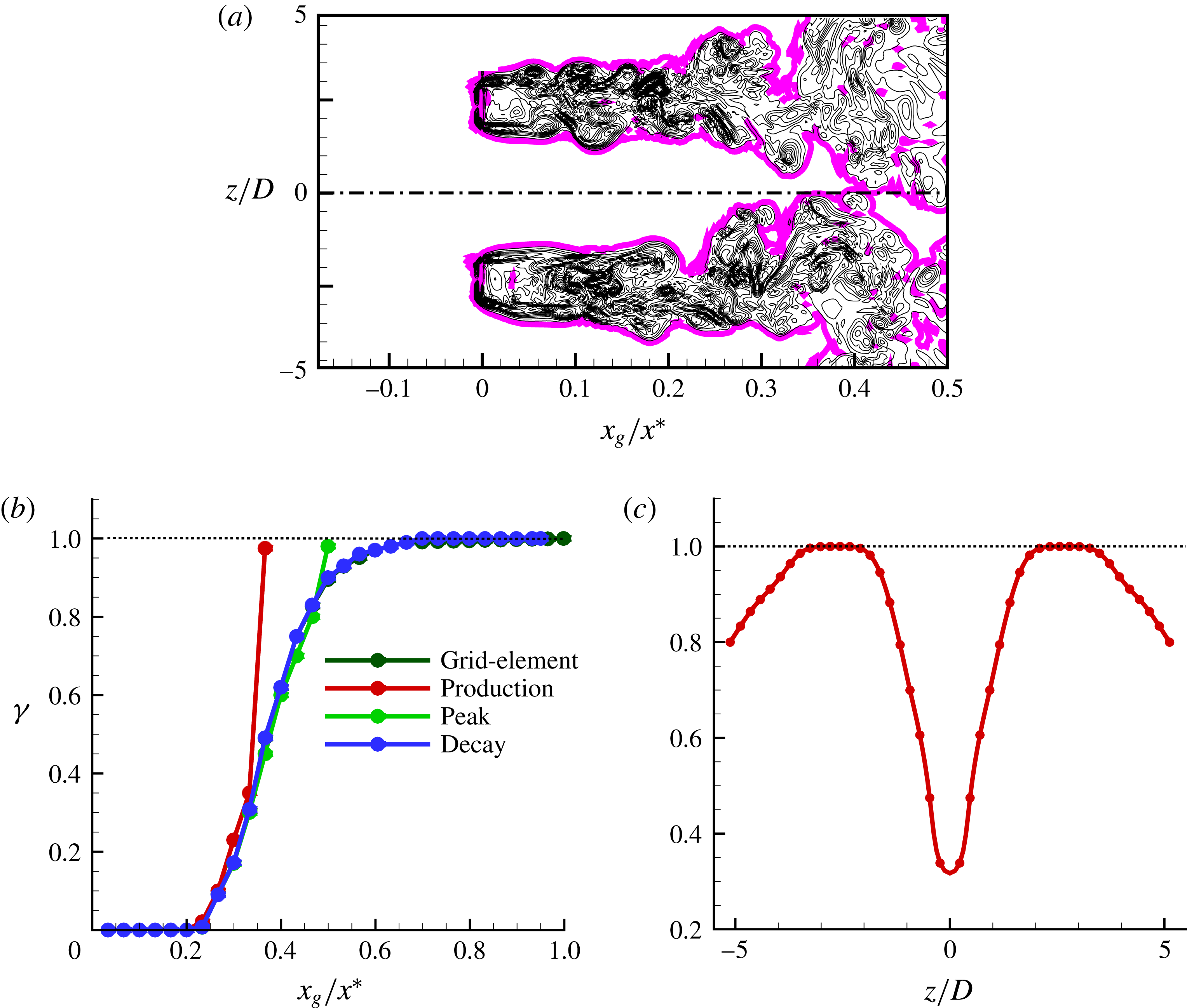
Finally, the intermittency of the oncoming turbulence is analysed. The study of intermittency is pertinent as the flatness of fluctuating streamwise velocity indicated that the production and peak regions are dominated by rare intense events. The intermittency factor ( $\unicode[STIX]{x1D6FE}$ ) is determined from the instantaneous magnitude of the vorticity vector ( $|\unicode[STIX]{x1D74E}^{\ast }|$ ), with components $\unicode[STIX]{x1D714}_{i}^{\ast }=\unicode[STIX]{x1D716}_{ijk}(\unicode[STIX]{x2202}u_{k}^{\ast }/\unicode[STIX]{x2202}x_{j})$ . Following studies on turbulent/non-turbulent interfaces (Bisset, Hunt & Rogers Reference Bisset, Hunt and Rogers2002; Taveira et al. Reference Taveira, Diogo, Lopes and da Silva2013; Watanabe et al. Reference Watanabe, Sakai, Nagata, Ito and Hayase2014; Zhou & Vassilicos Reference Zhou and Vassilicos2017), the flow is defined as turbulent when $|\unicode[STIX]{x1D74E}^{\ast }|$ is greater than a certain threshold, ${|\unicode[STIX]{x1D74E}^{\ast }|}_{th}$ . The intermittency factor is defined as $\unicode[STIX]{x1D6FE}$   $=$ probability of ( $|\unicode[STIX]{x1D74E}^{\ast }|\geqslant |\unicode[STIX]{x1D74E}^{\ast }|_{th}$ ). As can be seen from this definition, the vorticity threshold value plays a crucial role in determining the intermittency factor. The method adopted for estimating $|\unicode[STIX]{x1D74E}^{\ast }|_{th}$ in this study closely follows that of Taveira et al. (Reference Taveira, Diogo, Lopes and da Silva2013) and Zhou & Vassilicos (Reference Zhou and Vassilicos2017). Since this study focuses only on the grid-element centreline $z=0$ plane, a two-dimensional instantaneous vorticity slice with dimensions $0\leqslant x\leqslant 0.5x^{\ast }$ and $-5.3D\leqslant z\leqslant 5.3D$ is considered in this plane. A wide range of $|\unicode[STIX]{x1D74E}^{\ast }|_{th}$ values from 0 to 10 was considered. For each value of $|\unicode[STIX]{x1D74E}^{\ast }|_{th}$ , the fraction of turbulent area $A_{T}$   $=$ area of $(|\unicode[STIX]{x1D74E}^{\ast }|>|\unicode[STIX]{x1D74E}^{\ast }|_{th})/\max (A_{T})$ is computed. The variation of $A_{T}$ with $|\unicode[STIX]{x1D74E}^{\ast }|_{th}$ is depicted in figure 10(a). A plateau can be seen for a range of $|\unicode[STIX]{x1D74E}^{\ast }|_{th}$ values. It is generally believed that the intermittency factor weakly depends on $|\unicode[STIX]{x1D74E}^{\ast }|_{th}$ when the threshold is chosen to be in this plateau (Taveira et al. Reference Taveira, Diogo, Lopes and da Silva2013; Watanabe et al. Reference Watanabe, Sakai, Nagata, Ito and Hayase2014; Zhou & Vassilicos Reference Zhou and Vassilicos2017). This is checked in figure 10(b) which shows the variation of intermittency factor for various $|\unicode[STIX]{x1D74E}^{\ast }|_{th}$ . The profile of $\unicode[STIX]{x1D6FE}$ is found to be insensitive to $|\unicode[STIX]{x1D74E}^{\ast }|_{th}$ when $0.12\leqslant |\unicode[STIX]{x1D74E}^{\ast }|_{th}\leqslant 0.25$ . Therefore, we choose $|\unicode[STIX]{x1D74E}^{\ast }|_{th}=0.2$ .

The detected T/NT interface using this threshold value is visualised in figure 11(a). The figure shows that the vortical structures are enveloped by the interface. The value of $|\unicode[STIX]{x1D74E}^{\ast }|_{th}$ depends on the flow configuration. For example, Bisset et al. (Reference Bisset, Hunt and Rogers2002) reported a value of 0.7 for the far wake of a cylinder, while for a jet it is found to be 0.3 (Watanabe et al. Reference Watanabe, Sakai, Nagata, Ito and Hayase2014). The variation of intermittency factor along the grid-element centreline for all the cases is presented in figure 11(b). As can be seen, the region $0\leqslant x_{g}/x^{\ast }\leqslant 0.2$ is purely irrotational and the region $0.2\leqslant x_{g}/x^{\ast }\leqslant 0.5$ is intermittent. Note the rapid increase of $\unicode[STIX]{x1D6FE}$ for the production and peak cases in points situated inside the developing boundary layer on the surface of the cylinder. This analysis reveals that the oncoming flow is indeed highly intermittent for the production case, less intermittent for the peak case and fully turbulent for the decay case. Since the cylinder is placed at $x_{g}/x^{\ast }=0.35$ for the production case, we also need to quantify the intermittency factor along the spanwise direction for this particular case. This information is provided in figure 11(c) where one can note some intermittency of the order of $\unicode[STIX]{x1D6FE}=0.8$ in the region between $z/D=\pm 5.3$ and $z/D=\pm 4$ . As a result, we choose $z/D=\pm 5$ for further analysis in the rest of the paper besides the grid-element centreline for the production case. Therefore, we have intermittent flow both at the grid-element centreline (i.e. $z/D=0$ ) and at $z/D=\pm 5$ of the production case.

As an interim summary, the oncoming turbulence generated by the single square grid-element has the following characteristics downstream of the grid-element: in the production and peak regions, the turbulence is highly non-Gaussian, inhomogeneous and intermittent; on the other hand, at the decay region it is Gaussian, approximately homogeneous and fully turbulent.

4.1 Mean velocity and turbulent stress profiles inside the boundary layer

Figure 12.

Mean azimuthal velocity profiles inside the boundary layer in the $z/D=0$ plane (red, production; green, peak; blue, decay; purple, cylinder).

The azimuthal velocity profiles at different angles are compared in figure 12 for all cases considered. The variation in the radial direction, normal to the cylinder surface at plane $z/D=0$ , is plotted. The value of mean azimuthal velocity at the front stagnation, at $\unicode[STIX]{x1D703}=0^{\circ }$ , is zero due to symmetry. Moving clockwise, the velocity gradually increases. The boundary layer theory predicts that the thickness of the laminar boundary layer at the stagnation point ( $\unicode[STIX]{x1D6FF}$ ) has a power-law relationship with Reynolds number as $\unicode[STIX]{x1D6FF}/D=Re_{D}^{-0.5}$ (Zdravkovich Reference Zdravkovich1997). This relationship appears to be satisfied for the cases considered in this study, as the simulations indicate a boundary layer thickness of $0.05D$ at $\unicode[STIX]{x1D703}=0^{\circ }$ , a value close to the theoretical prediction. Despite being exposed to turbulent fluctuations, the boundary layer profiles of production, peak and decay cases are comparable to the cylinder case. This indicates that the boundary layer on the surface of the cylinder in all cases could be laminar. Indeed, Jones & Launder (Reference Jones and Launder1973) showed that the boundary layer remains laminar for acceleration parameter $K$ , defined as $K=(\unicode[STIX]{x1D708}/U_{\infty }^{2})(\text{d}U_{\unicode[STIX]{x1D703}}/\text{d}s)$ (where $\text{d}s$ is the circumferential distance on the surface of the cylinder) in excess of $2.5\times 10^{-6}$ . We measure $U_{\unicode[STIX]{x1D703}}$ at $r/D=0.7$ . The value of $K$ at $75^{\circ }$ is computed to be around $3.5\times 10^{-6}$ , a value close to the critical value. Therefore, the boundary layer flow in the range of $0^{\circ }\leqslant \unicode[STIX]{x1D703}\leqslant 75^{\circ }$ is not fully laminar.

Figure 13.

Hydrodynamic stress profiles inside the boundary layer in the $z/D=0$ plane: (a) radial stress, (b) azimuthal stress, (c) spanwise stress, (d) Reynolds stress (red, production; green, peak; blue, decay; purple, cylinder).

The turbulent stress profiles along the radial direction are plotted in figure 13. The stresses considered here are (i) radial stress ( $\langle u_{r}u_{r}\rangle$ ), (ii) azimuthal stress ( $\langle u_{\unicode[STIX]{x1D703}}u_{\unicode[STIX]{x1D703}}\rangle$ ), (iii) spanwise stress ( $\langle u_{z}u_{z}\rangle$ ) and (iv) Reynolds stress ( $\langle u_{r}u_{\unicode[STIX]{x1D703}}\rangle$ ). They are all normalised by $U_{\infty }^{2}$ . The effect of free-stream turbulence has penetrated inside the boundary layer, as the stress magnitudes are larger near the cylinder surface for the production, peak and decay cases while they are zero for the cylinder case. Within the boundary layer, the azimuthal and spanwise stresses are higher than the radial stress, due to the wall blocking that suppresses the latter. The magnitude of stresses gradually increases moving clockwise from the front stagnation point. The peak case exhibits the largest stress at all locations as its oncoming turbulence intensity is maximum. The radial and spanwise stress profiles collapse for the production and decay cases, especially for $\unicode[STIX]{x1D703}\geqslant 45^{\circ }$ . This is not the case however for the azimuthal as well as the Reynolds stress profiles.

Figure 14.

Variation of friction coefficient along the circumference of the cylinder in the $z/D=0$ plane.

The effect of free-stream turbulence on the skin-friction coefficient ( $C_{f}$ ) along the circumference of the cylinder is shown in figure 14. The mean separation angles, $\unicode[STIX]{x1D703}_{s}$ , for the cylinder, production, peak and the decay cases are computed to be 93.5, 100.2, 103.5 and 97 respectively. The higher values of separation angle for the production, peak and decay cases compared to that of the cylinder case signify the influence of free-stream turbulence in energising the laminar boundary layer and delaying its separation from the cylinder surface.

5.1 Mean temperature and turbulent heat-flux profiles inside the boundary layer

Figure 15.

(a) Mean temperature profiles inside the thermal boundary layer in the plane $z/D=0$ , (b) wall-normal turbulent heat-flux ( $|\langle u_{r}T\rangle |$ ) profiles inside the thermal boundary layer in the plane $z/D=0$ (red, production; green, peak; blue, decay; purple, cylinder).

Figure 15(a) shows the thermal boundary layer profiles at different angles. These profiles are normalised by $q_{w}D/k$ , where $k$ is the thermal conductivity. The thermal boundary layer is thicker than the hydrodynamic boundary layer, because $Pr<1$ and therefore the thermal diffusion is larger than the viscous diffusion. Indeed, the thickness $\unicode[STIX]{x1D6FF}_{T}$ is approximately $0.1D$ , which is twice the hydrodynamic boundary layer thickness, $\unicode[STIX]{x1D6FF}$ . The mean temperature profiles of the production, peak and decay cases exhibit larger gradients compared to the cylinder case, indicating larger heat transfer. Between production and decay cases, the former has clearly larger gradients, and therefore higher heat transfer rate is expected. These observations are verified in the time-averaged Nusselt number ( $\langle Nu\rangle$ ) profiles, presented in the following subsection.

The wall-normal heat-flux profiles ( $|\langle u_{r}T\rangle |$ ) are depicted in figure 15(b). The presence of the cylinder blocks the radial fluctuation $u_{r}$ , and therefore the heat transfer near the cylinder is mainly due to molecular diffusion (Wissink & Rodi Reference Wissink and Rodi2011a ). Moving clockwise from $\unicode[STIX]{x1D703}=0^{\circ }$ , the wall-normal region where turbulent fluctuations are active is expanding radially outwards from the surface. The maximum turbulent heat flux is observed in the peak case, as expected. Comparing the profiles of the production and decay cases, the decay case has larger turbulent heat flux than the production case.

5.2 Effect of free-stream turbulence on Nusselt number profiles

Figure 16.

Variation of mean Nusselt number along the circumference of the cylinder in the plane $z/D=0$ : (a) production, (b) peak, (c) decay.

The variation of mean Nusselt number, $\langle Nu\rangle$ , for the production, peak and decay cases is shown in figure 16(a–c) respectively. The $\langle Nu\rangle$ for the cylinder case is also plotted for comparison. The observations noted from the mean temperature and turbulent heat-flux profiles are reflected in the $\langle Nu\rangle$ . The heat transfer rate of the production, peak and decay cases is higher than that of the cylinder. The maximum increase of heat transfer at the front stagnation point occurs for the production case with a substantial $63\,\%$ rise. On the other hand, the peak case, which has a maximum oncoming turbulence intensity of 15 %, results in a $61\,\%$ increase. The decay case exhibits the smallest increase of $28\,\%$ , although the oncoming turbulence intensities of the production and decay cases are similar.

Table 2.

Effect of incident Reynolds number on stagnation point heat transfer coefficient.

It can be argued that the increase of the incident velocity for the production and peak cases can explain the observed heat transfer enhancement. Therefore, we need to account for the effect of different Reynolds numbers on the stagnation point Nusselt number, $\langle Nu_{0}\rangle$ . Table 2 compares the present $\langle Nu_{0}\rangle$ against the values predicted by theory using the correlation $\langle Nu_{0}\rangle =0.95Re_{D}^{0.5}$ (Krall & Eckert Reference Krall and Eckert1973). The cylinder case value of $\langle Nu_{0}\rangle$ is closer to that obtained by Krall & Eckert (Reference Krall and Eckert1973). The results also reveal that the effect of the present Reynolds number range is weak when there is no oncoming turbulence and, therefore, cannot explain the large increase predicted in the production region. The largest deviation from theory is observed for the peak case, and the smallest for the decay case. This observation is expected as the peak case has the highest oncoming turbulence intensity of all other cases. It is interesting, however, to note that the production case has much higher heat transfer increase than that of the decay case although both cases have a similar turbulence intensity value. Clearly, the difference in heat transfer enhancement is not due to differences in the incident Reynolds number. The reasons are explored later in this study by means of time scale separation analysis and examining the dominant frequency of the turbulent fluctuations.

The next important observation in the $\langle Nu\rangle$ profiles (figure 16) is the location of the maximum. The front stagnation point on the surface of the cylinder is expected to have the highest heat transfer rate. This is because the cold oncoming flow makes contact with the cylinder surface first on the front stagnation point. As the flow warms up, the rest of the cylinder surface is exposed to flow with higher temperature than the one that has impinged on the front stagnation point (Paul et al. Reference Paul, Prakash, Vengadesan and Pulletikurthi2016). This observation is valid only in the cylinder case, when there is no oncoming turbulence. When a turbulence-generating grid-element is introduced, figure 16(a–c) shows that the $\langle Nu\rangle _{max}$ is shifted around $45^{\circ }$ away from the front stagnation point. Similar observations have been noted in the experimental study of Magari & LaGraff (Reference Magari and LaGraff1994) and the semi-DNS study of Venema et al. (Reference Venema, Von Terzi, Bauer and Rodi2011). In those studies the cylinder was subject to wake turbulence generated by a small cylinder placed upstream. They concluded that the shift in $\langle Nu\rangle _{max}$ is due to the presence of the small cylinder which creates a wake deficit which in turn decreases the convective heat transfer at the front stagnation point. The study of Wissink & Rodi (Reference Wissink and Rodi2011a ,Reference Wissink and Rodi b ), where the wake generator was simulated in a precursor simulation and the turbulence data were imposed on the inlet of the domain, could not detect such a shift in $\langle Nu\rangle _{max}$ .

In order to gain more insight into the effect of flow on heat transfer, contour plots of $\langle Nu\rangle$ on the surface of the cylinder are shown for all the cases in figure 17. For the cylinder case, the $\langle Nu\rangle$ contour is uniform in the spanwise direction (figure 17 a) as expected. The presence of the vertical bars of the grid-element results in non-uniform distribution of $\langle Nu\rangle$ in the spanwise direction. This is attributed to the fact the local velocity, turbulence intensity and integral length scales vary drastically along the spanwise direction. As can be seen in figure 17(b), $\langle Nu\rangle$ attains its maximum value around $\unicode[STIX]{x1D703}\approx 45^{\circ }$ along the grid-element centreline. This feature is more prominent in the production case and becomes milder for the decay case. Since the grid-element centreline is not directly immersed in the wakes of the bars, there is no wake deficit, and so the argument of Venema et al. (Reference Venema, Von Terzi, Bauer and Rodi2011) cannot explain why the location of $\langle Nu\rangle _{max}$ is shifted from the front stagnation point. We propose a novel explanation for this observation in the next subsection.

Figure 17.

Contours of mean Nusselt number on the cylinder surface: (a) cylinder, (b) production, (c) peak, (d) decay. The isocontours range from 8 to 36.

Figure 17(b) also reveals yet another intriguing behaviour. We know that the oncoming flow characteristics at the grid-element centreline (i.e. $z/D=0$ ) and at $z/D=\pm 5$ of the production case are similar, meaning that both are intermittent, non-Gaussian and inhomogeneous. The only difference between these two locations (i.e. $z/D=0$ and $z/D=\pm 5$ ) is the turbulence intensity values. At $z/D=0$ , the oncoming turbulence intensity is 11 % while it is approximately 24 % at $z/D=\pm 5$ . On the other hand, $\langle Nu\rangle _{0}\approx 35.3$ at $z/D=0$ while it is only 25.1 at $z/D\pm 5$ . These values and figure 17(b) vividly reveal that neither the intermittent, non-Gaussian nature of the flow nor the turbulence intensity are the most important parameters for the heat transfer. Note also that although the turbulence intensity is very high along the bar centreline, in particular for the production case (see figure 21 a), the maximum $\langle Nu\rangle$ is not observed along the bar centreline, instead it is located at the grid-element centreline. These observations also testify that the flow along the grid-element centreline has some unique characteristics that cause higher heat transfer for a lower oncoming turbulence intensity. These unique characteristics are explored in §§ 7 and 8.

Finally, we can note that the $\langle Nu\rangle$ contour of the decay case, shown in figure 17(d), is non-uniform along the spanwise direction although the oncoming turbulence is similar to the one considered in the literature. It appears that the flow at the decay region is only approximately homogeneous and it still remembers the upstream condition. Due to this reason, non-uniformity in $\langle Nu\rangle$ is not fully vanished for the decay case. Note also that the experiments, that used regular grids to generate oncoming turbulence, placed cylinders after $x/x^{\ast }\approx 4$ from the grid. Therefore, their results cannot be compared with our result in figure 17(d) as we are still in the near field of the grid and the flow is not fully disconnected from the upstream conditions.

5.3 Factors causing the shift in the location of $\langle Nu\rangle _{max}$

Figure 18.

Probability density functions of Nusselt number at different locations along the circumference of the cylinder in the plane $z/D=0$ : (a) cylinder, (b) production, (c) peak, (d) decay.

The shift in the location of $\langle Nu\rangle _{max}$ from the front stagnation point is further explored through probability density functions (PDFs) of Nusselt number at various azimuthal locations, plotted in figure 18. The PDFs of Nusselt number for the cylinder case appear to be Gaussian with a near-perfect symmetry. The other cases exhibit an interesting behaviour. The PDF at the stagnation point appears to be near-symmetric with a Gaussian profile. Yet, for the region of $0^{\circ }<\unicode[STIX]{x1D703}\leqslant 45^{\circ }$ , the PDFs lose their symmetry with more skewness towards higher values of $Nu$ . The level of skewness increases from $\unicode[STIX]{x1D703}>0^{\circ }$ to $\unicode[STIX]{x1D703}\approx 45^{\circ }$ . After $\unicode[STIX]{x1D703}\approx 45^{\circ }$ , the PDFs again translate to a near-symmetric shape for the production, peak and decay cases. It appears that additional intense events occur in the region of $0<\unicode[STIX]{x1D703}\leqslant 45$ compared to the front stagnation point that cause the skewness of the PDFs. Such events can be more clearly seen in figure 19 where the PDFs of Nusselt number at the front stagnation point and at $\unicode[STIX]{x1D703}=45^{\circ }$ are compared. The green shaded areas in these figures represent the additional intense events occurring at $\unicode[STIX]{x1D703}=45^{\circ }$ . Note that the shaded area in these figure is largest for the production case, and progressively decreases in the peak and decay cases. These events cause the PDFs of Nusselt number to skew more towards higher values, resulting in a higher heat transfer rate at $\unicode[STIX]{x1D703}=45^{\circ }$ .

Figure 19.

Illustration of additional intense events occurring at the $\langle Nu\rangle _{max}$ point in the plane $z/D=0$ for the case of (a) circular, (b) production, (c) peak, (d) decay.

Having identified the presence of intense events at $\unicode[STIX]{x1D703}=45^{\circ }$ , the question now is what causes such events. The answer can be found in the oncoming turbulence profiles. It is known that the Nusselt number is primarily a function of Reynolds number, turbulence intensity and length scales. The length scales are not expected to change drastically in the limited range of $0\leqslant \unicode[STIX]{x1D703}<45^{\circ }$ . However, the profiles of mean velocity show that there exists a jet-like behaviour as discussed earlier. Therefore, the cylinder sees a much higher velocity at locations $0<\unicode[STIX]{x1D703}\leqslant 45$ as seen in figure 7 for $x_{c}/D=-1$ . Adding to that, the oncoming turbulence intensity is also highly inhomogeneous in the cross-stream direction with less intensity at the stagnation point and higher values away from it (see figure 8). Therefore, it is believed that the increase in local mean incident flow and its turbulence intensity at $\unicode[STIX]{x1D703}\approx 45^{\circ }$ compared to the front stagnation point is related to the additional intense events which in turn shift the $\langle Nu\rangle _{max}$ by $45^{\circ }$ from the stagnation point.