

The experimental method provides a highly efficient means for confronting theoretical models with reality in order to build and improve our understanding of nature. In an attempt to increase the scientific nature of their young discipline, psychologists adopted the experimental method as a way to systematically describe and study human behavior. For this enterprise, they needed to “measure variables objectively,” and “accurately infer that the observed pattern of results reflects what typically happens” (Mitchell & Jolley, Reference Mitchell and Jolley2007). In other words, they needed to use statistical quantitative techniques.
Statistical quantitative techniques are complex mathematical methods mainly used to draw linear relations between variables. These methods must be handled carefully in order to avoid biased conclusions and the creation of fallacious theories. However, the democratization of user-friendly software has trivialized them and created a hazardous situation, where the conditions necessary for the applied method may not be known to its users.
Three general issues are essential prerequisites for safely exploiting any statistical knowledge. First, statistical quantifying techniques themselves do not allow us to determine the causality between an independent variable and a dependent variable. They only help determine the existence of a relation between these two types of variables. It is therefore the goal of experimental designs to guarantee that results are due to systematic changes in the independent variable.
Second, statistical quantifying techniques do not allow us directly to prove that a treatment has an effect. They only help establish whether any observed difference between the experimental condition and the control condition can be due to chance (statistical significance). Based on this probabilistic estimation, researchers will decide to reject or not to reject the null hypothesis. If they do not reject the null hypothesis, they cannot draw any conclusion: a nonsignificant difference between two conditions can be due either to a treatment (Type II error) or to chance (correct decision). If they reject the null hypothesis, the researcher estimates that the chance that there was no effect is low enough to conclude that there was probably an effect (correct decision). However, it may still be possible that the researcher is mistaken in taking this decision (Type I error), and builds theoretical knowledge on an incorrect inference (there was actually no treatment effect behind the measured difference).
Third, statistical significance does not measure an effect size. Small differences in the dependent variable between experimental and control conditions might be highly significant, whereas large differences might be nonsignificant. Statistical significance tells us nothing about the size and importance of the treatment effect. It is therefore important to provide information about these features (Abelson et al., Reference Abelson, Rosenthal, Aiken, Appelbaum, Boodoo and Kenny1996).
Additional issues must also be considered to avoid creating fallacious knowledge as much as possible. In this article, we review the most salient and complex issues that are encountered when filtering the raw data, managing missing values, and analyzing the filtered data. We subsequently provide solutions and indicate references to help nonspecialists find additional guidance.
Because of text-length restrictions, we only consider the chronometric data type (reaction times [RTs]) and factorial designs,Footnote 1 both widely used in cognitive psychology, and three statistical techniques derived from the general linear model (GLM): analysis of variance (ANOVA), quasi-F, and multilevel modeling (MLM). Consequently, this article is a technical tutorial for analyzing RTs obtained through a repeated-measures factorial design.
The first section reviews issues about filtering, managing missing values, and statistical modeling. The second section provides a benchmark in which the accuracy of each statistical technique is investigated in various situations, defined by the amount of missing data, their distribution across conditions, and replacement schemes.
HOW TO PROCESS RTs OBTAINED WITH A FACTORIAL DESIGN
Raw RTs obtained experimentally contain useful information (related to the variable or variables studied), useless information (due to parasite variables), and random variations not caused by any variable. Furthermore, not all the measurements may have resulted in data, leading to a data set with missing values. Consequently, before analyzing and extracting any meaning from the data, a researcher must preprocess the raw data by appropriately treating unrelated information (filtering or robustness) and by finding a suitable way of managing the missing data.
Filtering
Filtering is a technical prerequisite imposed first by the use of the GLM to analyze Gaussian and quasi-Gaussian phenomena,Footnote 2 and second by the need to consider only the information related to the studied Gaussian phenomena (or useful information). If abnormal values (non-Gaussian values or outliers, corresponding to unrelated information) are kept, classical methods of analysis might be influenced to such an extent that they will lead to incorrect inferences. Hence, either the data must be filtered properly prior to the analysis, or one must use robust methods of analysis, which are little influenced by outliers (see the Robust Methods Section). We review various filtering procedures in the following subsections, and more will be found in Ratcliff (Reference Ratcliff1993) about the filtering of outlier RTs, and in Ulrich and Miller (Reference Ulrich and Miller1994) about the issue of data truncation.
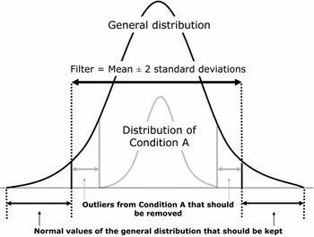
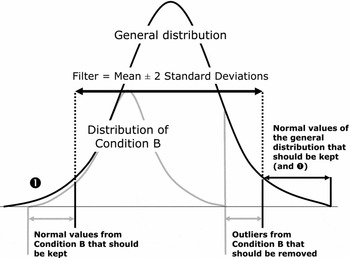
Standard filtering procedures. One of the standard filtering procedures used by psychologists consists in using all RTs and blindly eliminating values above and below the ±2 SD limits around the mean of the general distribution (grand mean). Although this filter erases some percentage of outliers, it also erases 4.66% of the Gaussian distribution. Furthermore, this type of filter can bias inferences, depending on the structure of the data, by not filtering all outliers in the distribution of a specific experimental condition, as well as by truncating the distribution of one or several condition(s). Four key scenarios are possible, depending on the one hand whether the grand mean (general distribution's mean) is similar or not to the mean of a specific condition (subdistribution's mean), and in contrast, whether the range of a specific condition's subdistribution tends to be large or small. Two out of these four scenarios are illustrated in Figure 1 (the mean of a subdistribution A equals the grand mean of the general distribution G) and Figure 2 (the mean of a subdistribution B differs from the grand mean). In both cases, subdistributions A and B have a smaller range than G.
Filtering the general distribution with a ±2 SD filter when the mean of Condition A equals the grand mean.

Filtering the general distribution with a ±2 SD filter when the mean of Condition B differs from the grand mean.

In Figure 1, filtering the overall distribution with a ±2 SD rule results in the loss of information from the general distribution (extreme left and right parts) and leaving possible outliers in the condition A subdistribution (center right part). Although the means of the general distribution and of condition A will not be modified by the filtering procedure, the variance of the overall distribution or total variance will be reduced, whereas the variance of condition A or intragroup variance will remain unchanged. Consequently, the ratio between intragroup variance and intergroup variance will be altered, and the significance of effects will be spuriously modified, probably diminished.
For situations as depicted in Figure 2, filtering the overall distribution with a ±2 SD rule will result in asymmetrically losing genuine values on the left side of the B subdistribution and asymmetrically leaving outliers on its right side. Consequences are numerous and much more serious than in the situation depicted in Figure 1: the filtering procedure not only spuriously reduces the variance of condition B but it also biases its mean toward the grand mean, turns its distribution non-Gaussian, reduces its area, and asymmetrically leaves outliers. Theoretically, each one of these five modifications is sufficient in itself to influence the inferential tests done on the filtered data. Their combined influence is highly unpredictable, and the resulting p values might be unreliable. The aforementioned biases are probably increased for the interaction terms. Because a ±2 SD blind filtering procedure applied on the overall distribution does not take into account the general distribution's composition into its subparts, thus leaving the possibility to keep outliers, eliminate information, and distort the distribution, it should be avoided or handled with great care. The minimum requirement would be to have all these points in mind and doublecheck them. A possible adjustment could be to increase the filtering precision by applying it to finer levels (each subject's distribution and item's distribution) instead of applying it to the grosser levels (whole distribution or distribution per condition). However, doing so requires a large number of measurements per item as well as per subject, in order to be able to correctly define the characteristics of the distribution and find out precisely which values must be filtered.
Because it is legitimate to wonder if results are an undesirable consequence of incorrect filtering procedures, a sensitivity analysis should be performed to check if the application of a filter is correct, necessary, or problematic. The principle of sensitivity analysis is to run the same analysis (ANOVA, regression, etc.) on the unfiltered data set as on the filtered data, for instance, with a ±2 SD rule, or preferably with a by subject and by item ±3 SD rule. If the significance tests yield similar results with the unfiltered and the filtered data sets, one can be more confident that the findings are not produced by filtering. Results should be reported for one of these analyses, mentioning that they were confirmed with a sensitivity analysis. By contrast, if results differ between analyses, one must investigate more thoroughly the reason why. Is it due to the elimination of outliers from the original data set, in which case the filter has correctly fulfilled its role, or is it because some distributions have been truncated, in which case the filter has introduced a bias? In this last situation, one should not interpret any result before a more careful analysis has been carried out, for instance through robust methods.
Robust methods
Robustness is a general term encompassing a complete methodology providing all the steps needed for an analysis: diagnostic, estimation, inference, and testing. Robust methods are procedures that are not or little influenced by outlying observations, or more generally by the misspecification of a model. They correctly describe the bulk's structure of data without requiring a prior filtering, by automatically downweighting the problematic observations (Courvoisier & Renaud Reference Courvoisier and Renaud2010; Maronna, Martin, & Yohai, Reference Maronna, Martin and Yohai2006; Wilcox, Reference Wilcox2005).
This methodology has several additional advantages. First, diagnostic plots provide subtle information showing which points were downweighted and to which extent. Second, it helps detect multidimensional outliers that are not detected by a unidimensional filter, like the ±2 SD rule (Maronna et al., Reference Maronna, Martin and Yohai2006).
A full robust methodology exists for regression, variable selection, simple, and factorial ANOVA (no repeated measure), and methods based on the variance–covariance matrix (principal component, factor analysis). It is implemented in some statistical software, like TIBCO Spotfire S+ (formerly S-Plus, TIBCO Software Inc., 2008), R (R Development Core Team, 2010) and SAS (SAS Publishing, 2000). In SPSS, there is no build-in robust procedure. However, a general SPSS plug-in to run R functions, including all robust procedures, can be downloaded from the company website. For repeated-measure and mixed-effects models, the full robust methodology is not yet available. However, robust procedures can still be used for the restricted sake of outlier detection. Actually, filtering data by using the arithmetic mean as a center estimator of a distribution and standard deviation as a measure of variability around the mean creates its own paradox: outliers have an enormous influence on the tools used to detect them, that is, mean and standard deviation. It is therefore much safer to proceed with measures of center and variability, little influenced by outliers, which are respectively known as robust estimates of center (M-estimators, e.g., the median; called rob-center here), and robust estimates of variability or scale (e.g., the median of the absolute deviation, MADFootnote 3; called rob-scale here). Research and applied work have provided estimates, called M-estimators, that keep the precision properties of the mean/variance in pure Gaussian data and the robustness of the median/MAD in the presence of outliers (Maronna et al., Reference Maronna, Martin and Yohai2006).
In a practical sense, it is recommended to use both robust and efficient M-estimators, like the Huber type and Tukey bisquare. Their only disadvantage is that a computer program is needed to handle them.
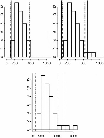
Filtering with rob-center ± 2 rob-scale or rob-center ± 3 rob-scale (global filtering or filtering by subject and by item) through a robust estimator will therefore more securely detect outliers than a classical ±2 SD or ±3 SD filter. Figure 3 illustrates this issue by comparing the outliers’ detection performance of a mean ±2 SD filter and of a rob-center ±2 rob-scale filter in three RT distributions. The left distribution is the reference data set prior to any addition of outliers, and the second and third distributions are respectively added with a small number of outliers and with a medium number of outliers.
A comparison of classical and robust filtering. Solid vertical lines = mean ±2 SD filter. Dotted lines = rob-Center ±2 rob-scale filter.

Because the initial distribution is loosely symmetric, the robust estimates (rob-center = 335.9, rob-scale = 117.5)Footnote 4 are very close to the classical estimates (mean = 336.6, SD = 111.7). Because the robust filter is less influenced by outliers than the classical filter, it rejects outliers more efficiently (second and third distributions) and is not dramatically changed between the three graphs.
For more on the general theory of robust statistics and its applications, the reader is referred to Maronna et al. (Reference Maronna, Martin and Yohai2006) and Wilcox (Reference Wilcox2005). The software described above allows for robust methods, and their user manuals, which are available on the Internet, are also good references.
Summary: How to filter data
We have shown that blindly filtering a data set can be as harmful as leaving outliers in a distribution. To strengthen the results’ reliability, a minimum requirement is to adjust the level of filtering from the whole distribution or from the distribution per condition to the distribution by item and by subject. It is even better to run a sensitivity analysis, which will let you know if filtering was necessary and if filtering did not introduce a bias. Another possibility is to use a robust method for filtering data before running the analysis. However, it is preferable to use fully robust methods, if they are available for the type of analysis that is planned (e.g., regression), for diagnosing, estimating, inferring, and testing the data set. Analyses might then be run without the need to filter extreme observations.
MANAGING MISSING VALUES
Correctly managing incomplete data sets is not an easy task. It cannot be automated because the procedure to be applied will depend on the reasons behind missing values. However, depending on these reasons and on the statistical technique chosen for analyzing the data, researchers may find themselves unable to escape this issue. They will generally need to apply a replacement procedure or use a statistical technique that allows for the given incompleteness.
Incomplete data sets are found in two situations: when the experimenter has decided not to use a complete experimental design in his study (incomplete by design: complex designs, technical constraints, inclusion of continuous independent variables), and when the researcher has planned a complete experimental design but ended up with some missing outcomes (missing values: measuring problems on some items, nonresponding of a participant on some trials, filtering). This section will focus on the management of missing values. First, the possible causes of the missing values will be presented. Second, the different replacement methods will be explored. Third, further details will be given concerning the situations where missing values can and must be replaced.
Possible causes of missingness: Missing completely at random (MCAR), missing at random (MAR), and not MAR (NMAR)
Data may be missing for various reasons, and therefore the appropriate solution will vary. Data are said to be MCAR when missingness is not systematically related to any variable (e.g., a random problem in the recording device or a momentary distraction of a participant), that is, any reason unrelated to the difficulty of the item, the experimental condition, or the quality of the participant. If a pattern exists in the distribution of missing values (i.e., more filtered values in an experimental condition or with an item), values are not MCAR and are either MARFootnote 5 or NMAR; the difference is that MAR values can be predicted from the information at one's disposal, that is, available data and covariates. For instance, if the items with the largest amount of filtered data are also the items with the longest RTs, it is likely that the probability of missingness depends on the items’ difficulty. Just as for MAR values, NMAR values are caused by some systematic process, but the missingness pattern cannot be recovered from the available data. For instance, this might be the case in a clinical survey that tests sick patients on a regular basis: it often happens that people will abruptly opt out of the testing if their health deteriorates, and thus the reason for not participating, which produces a missing value, is directly related to an unobserved increase of the dependent variable. If an additional predictor could be added to model health deterioration, the missingness mechanism would be described and therefore would become a MAR type. The seminal reference for missingness types is Little and Rubin (Reference Rubin1987; see also Schafer & Graham, Reference Schafer and Graham2002).
The suitability of a given replacement method depends on two aspects: the type of missingness (MCAR, MAR, or NMAR) and the type of analysis that will be carried out (ANOVA type or multilevel). In case of MCAR values, four solutions are valid. The first and easiest solution is to delete any subject and any item with at least one missing value in order to allow a complete-case analysis. This is, for example, the default strategy used in SPSS for repeated-measure ANOVAs. The second solution is to use an accurate replacement procedure like the expectation–maximization (EM) algorithm and the multiple imputation (MI) algorithm. Replacing missing values with a mean by subject and item, a third possible solution, will probably lead to similar results. The fourth and final solution is to work directly on the data likelihood, as in the MLM, which does not require complete designs (see the MLM Section). Note that even though all of the above solutions are correct regarding the Type I errors in case of MCAR values, some of these solutions are much more powerful regarding Type II errors. For instance, deleting subjects or items will result in a proportional loss of information, making this solution less powerful than replacement methods and MLM.
MAR encompasses a large number of situations in psychology. The complete-case analysis is not valid in these situations. For instance, in a study comparing an experimental group of cognitively impaired patients with a control group of normal individuals, the task might be slightly too difficult for the experimental group but not for the control group. Consequently, the weakest patients might be more likely to answer incorrectly more often than the healthier patients. In this situation, removing subjects with at least one missing value will result in erasing the data from the weakest patients, therefore artificially modifying the mean for this group and biasing the information of the study. In contrast, the other three solutions given for processing MCAR values are still valid for processing MAR values.
In case of NMAR values, none of the methods discussed in this article are suitable. The only correct approach is to model the probability of a nonresponse, which goes beyond the scope of this article (see Little & Rubin, Reference Little and Rubin1987).
Methods for missing values replacement
Five methods for missing values replacement are examined in this section: replacement by the grand mean of the data set, by a mean per condition, by simple extrapolation using a “by item” and “by subject” mean, by extrapolation with linear regression, and by extrapolation with EM and MI algorithms.
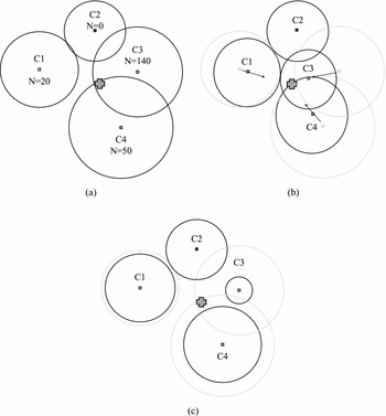
To better illustrate the impact of a replacement scheme on the results of a study, visual representations will be used in the following sections. The first type of representation (Figure 4a–c) uses abstract concepts from physics (center of gravity and area) as a metaphor of statistical concepts (respectively mean and variance), in order to give to the reader an intuitive picture of the distortions that replacement methods may cause on means and variances, therefore on statistical results.Footnote 6
The influence of replacement schemes on the mean and dispersion of conditions around the grand mean. C, conditions; N, amount of missing values per condition; crosses, grand mean; squares, means of conditions; circles, dispersion of the data around the mean of a condition. (a) Original distribution and (b) dispersion before (gray dotted circles) and after (black solid circles) the replacement of missing values by the grand mean. Arrows show the drift of the means toward the grand mean for the conditions having missing values (C1, C3, and C4). (c) Dispersion before (gray dotted circles) and after (black solid circles) the replacement of missing values by the mean per condition. Only the dispersion is modified here.

In Figure 4a, each one of the four represented conditions (C1–C4) should contain the same amount of measurements, that is, 200. However, three conditions (C1, C3, and C4) have N values missing (20, 140, and 50, respectively), as is likely to be the case in a real experimental situation. Depending on the proportion of missing values per condition, some conditions (like C3, a high proportion of missing values) are likely to be affected more than others (like C1, a small proportion of missing values) by the replacement procedure, depending on the procedure (Figure 4b and c). By contrast, the condition C2 will not be influenced by any replacement procedure because it has no missing values.
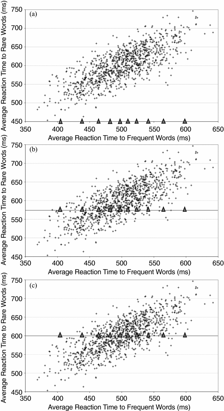
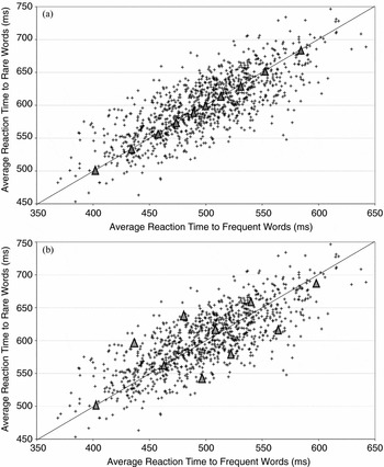
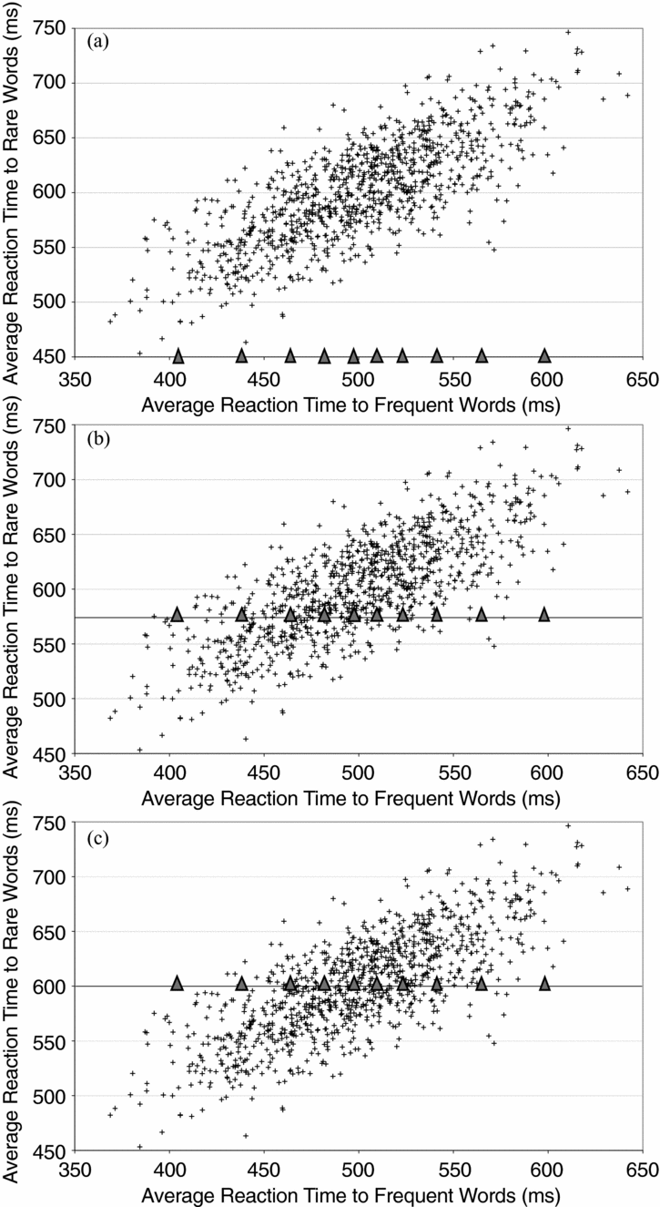
The second type of representation (Figure 5a–c and Figure 6a–b) uses a classical scatter plot to illustrate how the replacing values will modify the distribution. This representation is based on psychological data (RTs), distributed in one condition according to another.
The influence on the conditions’ distribution of simple replacement schemes. (a) Initial distribution before applying a replacement scheme, (b) replacement by the grand mean, and (c) replacement by the mean per condition. Scatterplots show the distribution of subjects’ averaged reaction times in one condition (rare words) depending on the other (frequent words). Triangles represent missing values in (a) and the replacing values in (b) and (c). To simplify the graph, values were only missing in the “rare words” condition.
The influence on the conditions’ distribution of more advanced replacement schemes. (a) Replacement by regression prediction and (b) replacement by extrapolation with the multiple imputation algorithm.

Figure 5a shows the simulated distribution of subjects’ averaged RT during the recognition of isolated words. Averages are plotted according to two conditions (RT for rare words vs. RT for frequent words), each cross-corresponding to the average performance of one subject in both conditions. In this example, missing values existed only in the Rare Words Condition. They are represented as triangles on the x axis. Figure 5b and c shows how the replaced values are distributed after applying simple replacement schemes, respectively, a replacement by the grand mean and a replacement by the mean per condition.
Replacing the missing values by the grand mean. Figure 4b shows that replacing missing values by the grand mean compresses the intragroup variances: for each condition, the dispersion around the mean (solid circles) is reduced compared to the original distribution (dotted circles). It also shows some compression of the intergroup variances: in each condition, the center of gravity has drifted toward the grand mean (arrows), distorting the relation between conditions. Therefore, replacing the missing values by the grand mean not only distorts the main effects, it also distorts interactions. Figure 5b shows that replacing missing values by the grand mean artificially lowers the correlation between conditions and introduces observations outside of the initial distribution. The consequences of this replacing scheme are an increased risk of Type II error (losing existing main effects) as well as of Type I error (nonexistent interactions become significant). Although replacing missing values by the grand mean is a common procedure, technically simple, and offers the advantage of eliminating weak main effects, we do not recommend using it, especially if the study intends to make theoretical conclusions about interactions. See the benchmark section for a test of this replacement scheme.
Replacing the missing values with a mean per condition. Replacing missing values with a mean per condition compresses the intragroup variance (dispersion around means is reduced) without compressing the intergroup variances (no drifting of the means toward the grand mean; see Figure 4c). Looking at the relationship between two experimental conditions (Figure 5c), this replacement scheme allows for replaced observations that are outside the bulk of the initial distribution. Although this type of replacement may appear to be superior to a replacement by the grand mean, it is actually not the case: it can create main effects as well as interactions, and therefore lead to Type I errors; consequently, it should be disregarded as well. See the benchmark section for a test of this replacement scheme.
Extrapolating the missing values with means by subject and item. Any missing value can be replaced by a mean extrapolated from all the responses of the subject showing this specific missing value and all the responses for the item showing the same specific missing value. This extrapolation is computed according to Equation 1:
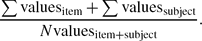
Replacing missing values by a mean will always cause variance reduction and a distortion of the original distribution. However, the distortion of information in the data set is often less important with extrapolated means than with the grand mean or the means per condition. See the benchmark section for a test of this replacement scheme.
Extrapolating the missing values with a linear regression. A more sophisticated method to extrapolate the missing values from existing observations is to use a regression analysis, in order to predict the missing values existing in one condition from the values existing in another condition. This situation is depicted in Figure 6a.
Replacing the missing values with a regression estimate artificially increases the overall correlation between two conditions. This leads to an overestimation of the effect, reducing the p value (Type I error artificially low), and finally causing the test procedure to be too liberal. Hence, another solution must be considered.
Extrapolating the missing values with the EM and MI algorithms. Two gold standards for completing data sets with missing values are based on algorithms: the EM algorithm (Dempster, Laird, & Rubin, Reference Dempster, Laird and Rubin1977) and the MI algorithm (Rubin, Reference Rubin1987). We will sketch only the principles behind each method, referring the reader to Schafer and Graham (Reference Schafer and Graham2002) for an excellent and detailed review.
The EM algorithm internally replaces the missing values and applies the analysis procedure, providing new values with optimal properties for the testing procedure (i.e., see the SPSS Missing Value add-on module, the SAS STAT base package, or the S-Plus Missing Base Library). The MI algorithm also completes data sets based on the characteristics of the existing data (mean, scale, skewness). Figure 6a showed that extrapolating the missing values based on a linear regression underestimated or overestimated their correlation with the existing data. Therefore, the missing values must be predicted by adding to the regression estimate the same amount of imprecision that exists in the real data (Figure 6b). Analyzing data sets completed with this procedure results in an optimal inferential test, that is, neither too conservative nor too liberal. Formally, the bias of the test procedure is accurate. However, the imprecision (random perturbations) artificially added to the predicted values increases the variance of the estimators. This problem is corrected with the MI procedure of the MI algorithm, which runs the same algorithm T times on the initial data set (typically T = 20). Because of the imprecision added to the predictions and the different tests at each run, an average of all runs provides a more reliable estimate by neutralizing noise. After data set completion, usual analysis procedures (like ANOVA) can be applied. All of these strategies for missing values replacement will be benchmarked in a later section, together with some methods that do not require replacing missing values, also described below.
STATISTICAL MODELING
The structure of information in factorial designs: An introduction to levels
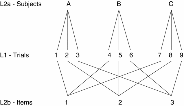
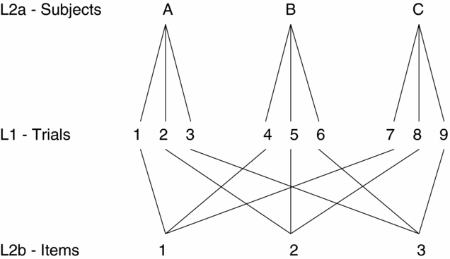
In the discussed factorial designs, the same subject will process a series of items, which are themselves presented to a set of subjects. Such a situation includes one or several fixed sources of variance: the experimental factors, and possibly additional factors that need to be controlled statistically. Usually, there are two random factors: subjects and items. These two random sources of variance can be crossed or nested. If, for example, items are words, items, and subjects can be considered as crossed because all the members of a linguistic community share the same words to communicate. In this case, one accepts the hypothesis that every subject will react the same way to the same word. The design of this cross-level structure is depicted in Figure 7: the two random factors are at the same level (2a and 2b), and their crossing is the experimental measurement or trials (Level 1, experimental factors are not represented). In this situation, the characteristics of both the subjects and the items influence the experimental measurement (trials).
The structure of information with two crossed random factors (here with three subjects [A, B, and C] and three items [1, 2, and 3]).
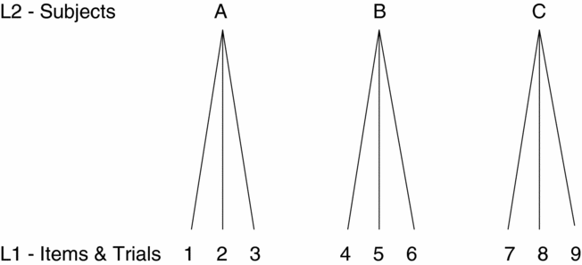
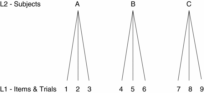
It is also possible that each individual builds his/her own mental representation of words, or has a different organization of his/her mental lexicon than any other individual, for instance, because of personal history. In this case, every subject may have a different reaction to the same word. Items, which are not words but rather mental representations of words, are nested within subjects. The design of this hierarchical-level structure is depicted in Figure 8: the experimental measurement (trials) is now confounded with the items level (Level 1), items are considered as different for each subject (nesting), and subjects compose the upper level (Level 2).
The structure of information with two hierarchical random factors (three subjects and three items).
Statistical models are approximations of reality, even for simple designs: “All models are wrong, but some are useful” (Box, Reference Box and Wilkerson1979). Therefore, in this example with words, the reality probably lies in between cross-level and hierarchical-level structures, as words are crossed with subjects whereas their representation is both crossed with subjects (universal properties) and nested within subjects (personal experience of words).
Processing levels with statistical techniques: Quasi-F and MLM
An important characteristic of factorial designs in psychology, multiple randomness, is caused by the simultaneous existence of items and subjects in the experimental situation, which will correspond to levels of random variance in the data. Analyzing data with multiple levels of random variance can be handled with the quasi-F approach or with the MLM technique. By contrast, a repeated-measure ANOVA and a classical F1 + F2 testing procedure are not directly able to handle multiple random factors in the data. Therefore, this last approach is not recommended for analyzing factorial designs. Quasi-F and MLM are presented in the following two sections. Issues with the use of ANOVA coupled with a classical F1 + F2 testing procedure will be discussed in the Quasi-F Section.
F′, F1 + F 2, and minF′ procedures. In a situation where two random factors exist, running two separate ANOVAs on the same set of data (F1 + F2 procedure), with each analysis modeling one random factor at a time, will result in conflating the variance of the remaining unmodeled random factor with the modeled random factor as well as with the fixed variance. This happens because the statistical model is underspecified. The danger in such a case, as already pointed out in the early 1970s (Clark, Reference Clark1973), is an increased risk to underestimate a Type I error, the F1 + F2 procedure not guaranteeing that the fixed effects can be generalized both to all the possible subjects and all the possible items at the same time. The only proper way to process data containing two random factors like items and subjects is to specify correctly the statistical model by including all the sources of variation in the equation.
A first way to solve the limitations of the repeated-measures ANOVA is to compute a quasi-F ratio instead of an F ratio (Clark, Reference Clark1973; Kirk, Reference Kirk1968; Winer, Brown, & Michels, Reference Winer, Brown and Michels1991). Actually, in a situation where two random factors are present simultaneously, the test for the fixed effects cannot be obtained with an exact F ratio. Equation 2 models a simple situation where subjects and items are crossed and one experimental factor is manipulated:

where i is subjects, i = 1, . . ., r; j is items, j = 1, . . ., q; k is treatments, k = 1, . . ., p; μ is the grand mean; α is the main effect of the treatment (T); βj (k) is the main effect of the word in the treatment [W(T)]; πi is the main effect of the subject (S); απjk is the Treatment × Subject (TS) interaction; πβij (k) is the Subject × Word interaction in treatment (W(T)S); and ɛ0(ijk) is the experimental error.
Computing a quasi-F ratio or F′ implies decomposing the total variance into its source components, in the form of sums of squares and mean squares (MS). In the design corresponding to Equation 2, these mean squares are MST for treatment, MSW (T) for word (embedded or nested within treatment), MSS for subject, MSTS for the Treatment × Subject interaction, and MSW (T)S for the Word × Subject interaction. No regular F test as would be computed in a factorial ANOVA with repeated measures can be built from these MSS (Clark, Reference Clark1973), precisely because two random factors (Subject and Word) are in the design. However, an F′ ratio (Equation 3) proves to be a good alternative to measure the importance of a treatment effect:
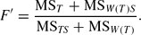
Although the distribution of F′ is not an exact F distribution because it is composed of four MS rather than two, it is close to an F distribution (hence, the term quasi-F).Footnote 7 Its degrees of freedom (df) are approximated by Equations 4 and 5.


Some authors have criticized this method as being too conservative (Wike & Church, Reference Wike and Church1976), but it seems to be an unfair statement, as shown by Forster and Dickinson (Reference Forster and Dickinson1976), Raaijmakers et al. (Reference Raaijmakers, Schrijnemakers and Gremmen1999), and our own experience (see the benchmark section). However, a first disadvantage is that this method cannot be applied directly with unbalanced designs or missing values. Inevitably, a replacement scheme must be used. A second disadvantage is that this method becomes more complex for more advanced designs, and is not available in the popular statistical packages. Renaud and Ghisletta (2007) provided a formula for all designs with more than one factor, together with an S-Plus library, to compensate for this flaw.
A significant quasi-F means that a treatment would also be significant in another experiment with both a different set of subjects and a different set of items. In other words, a significant effect obtained with quasi-F can be generalized to any group of subjects and to any set of items, which is yet the milestone of statistical tests. However, because of the two drawbacks described above, the F1 + F2 testing method was adopted as a consensual custom in some fields of psychology.Footnote 8 It consists of running two separate ANOVAs on the same set of data, each analysis considering a different random source of variance, by subjects (F1) or by items (F2). It is easy to show that this double testing procedure may not systematically lead to the correct generalization. It can only demonstrate that another experiment with a different set of subjects and the same set of items would yield the same results, and another experiment using the same set of subjects and a different set of items would yield the same results. The F1 + F2 procedure alternatively denies the existence of one random source of variance, and conserves only one random source in the analysis, instead of modeling both of them simultaneously. Note that the F1 + F2 testing procedure acknowledges the existence of two random factors but is not structured to analyze the situation appropriately.
According to Forster and Dickinson (Reference Forster and Dickinson1976, p. 135), Type I errors because of this procedure would occur more frequently than suspected in the scientific literature: “In extreme cases, the Type I error rates for F1 and F2 can exceed the desired rate by a factor of at least 10.” For technical issues and a complete discussion, see Clark (Reference Clark1973, Reference Clark1976), Raaijmakers et al. (Reference Raaijmakers, Schrijnemakers and Gremmen1999), Forster and Dickinson (Reference Forster and Dickinson1976), or Wike and Church (Reference Wike and Church1976).
Finally, Clark (Reference Clark1973) introduced a lower bound for F′, hence called minF′. It implies that if minF′ is significant, one is sure that F′ will be significant as well, however, if minF′ is not significant, one cannot infer on F′. The advantage of minF′ is that Clark (Reference Clark1973) has shown that it is easily computed:
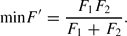
Its degrees of freedom are given by df num = p − 1 and df denom is the same as Equation 5, but it can be computed alternatively as

Therefore, if minF′ is used as a criterion, it will be more conservative than F′. Clark (Reference Clark1973) advises that it should be used only when F′ cannot be computed, and explicitly states (p. 348) that it is “far preferable” than F1 + F2.
MLM. “Multilevel analysis is a methodology for the analysis of data with complex patterns of variability, with a focus on nested sources of variability: e.g. pupils in classes, employees in firms, . . .” (Snijders & Bosker, Reference Snijders and Bosker1999). The MLM technique is an extension of the regression technique, for which the ANOVA is a particular case. Its development in the 1980s (Goldstein, Reference Goldstein2003) was mainly initiated by the need for modeling mixed effects and the influence of context in the field of social sciences. “Historically, multilevel problems have led to analysis approaches that move all variables by aggregation or disaggregation to one single level of interest, followed by an ordinary multiple regression, analysis of variance, or some other ‘standard’ analysis method. . . . Analyzing variables from different levels at one single common level creates two different sets of problems” (Hox, Reference Hox2002). These two problems are the aggregation and the disaggregation of data. From a statistical point of view, aggregating data (merging information from Level 1 in Level 2) will result in a loss of information and in a decrease of power of the analysis. Using the F1 + F2 procedure, for instance, drives to aggregate levels by averaging over items or over subjects. On the contrary, disaggregating results from ignoring the existence of a Level 2; therefore, conflating information from Level 2 with information from Level 1, for example, allocating subject variability to the measurement level (Level 1) can possibly lead to significant effects that do not exist.
MLM allows for specifying the different sources of variance in the model, for fixed factors as well as for random factors. Researchers can therefore draw a more exact schema of variance sources in the situation they are studying, from any level as well as between levels: main effects, simple and complex interactions, covariates effects. MLM offers enough flexibility to elaborate complex and realistic mathematical models and do not require balanced designs. It therefore automatically accommodates to MCAR and MAR situations by simply using all the available data. The necessary amount of data, even to analyze complex situations, is not excessive compared to other techniques like structural equation modeling. Finally, an important asset of the technique for psychologists is its ability to separate precisely and accurately the variance because of an experimental factor, from the variance due to unknown, and therefore unmodeled, parasite factors (cross-level models).
Software that models mixed effects (R, S-Plus, SAS, SPSS) and software dedicated to MLM (MLwiN) can be used; see the MLwiN manual for further information or one of the following references (Baayen, Reference Baayen2008; Goldstein et al., Reference Goldstein, Rasbash, Plewis, Draper and Yang1998; Rasbash, Steele, Browne, & Prosser, Reference Rasbash, Steele, Browne and Prosser2005; Renaud & Ghisletta, 2007; Snijders & Bosker, Reference Snijders and Bosker1999).
Comparing the structure of multilevel models: Cross-level models and hierarchical-level models
In a cross-level model with two random factors, the two random factors locate at the second level in the structure, and the first level results from the crossing of the two random factors, as shown in Figure 7. Therefore, the variance at Level 2 is caused by the differences existing between items and between subjects. The variance at Level 1 is due to measurement errors and any other source of variation not included in the model (residual error).
In a hierarchical-level model, items are located at Level 1 in the structure and are nested within subjects at Level 2, as shown in Figure 8. The variance at Level 1 is due to the differences between items, measurement errors, and residual error. The variance at Level 2 is due to the differences between subjects. Fixed factors like “Treatment” are included in these models as covariates.
While comparing the performance of cross-level and hierarchical-level models on a set of real data (taken from a lexical decision task experiment investigating the recognition of isolated spoken words) we found that the fit of a model to the data, estimated with the iterative generalized least squares algorithm (Rasbash, Reference Rasbash1992), was better with cross-level models than with hierarchical-level models. However, if enough covariates were added in the model for explaining the items, like word frequency, word length, concreteness, and so forth, the fit of the two types of models tended to converge.
Performance of the different statistical analysis methods
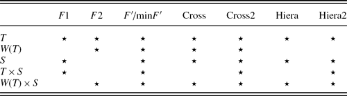
Behavioral data from a real experiment studying the perception of language according to the factorial design described in the example above (two random factors and one fixed factor) were used to compare the outputs provided by the various techniques described above: ANOVA by subjects (F1), ANOVA by items (F2), quasi-F (F′), minF′ (minF′), cross-level model (Cross), and hierarchical-level model (Hiera). It is important to note that even in this very simple design, MLM allows adding a “hybrid” term, the T × S interaction. This term, which can be understood as a random slope, is traditionally not incorporated in multilevel models, although it is incorporated in ANOVAs and quasi-F.Footnote 9 Consequently, to allow a direct comparison between MLM and quasi-F, two additional multilevel models were also tested: Cross2 and Hiera2. These two models were obtained by adding the interaction term T × S respectively to the Cross and Hiera models. Methods F′ and Cross2 are based on the same model, but they vary in their ways to test significance. Terms in the equation of each model are given in Table 1.
Terms included in each model
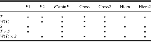
Note: W(T) × S is (confounded with) the residuals. Cross and Hiera are cross-level and hierarchical-level models. Cross2 and Hiera2 are the corresponding models including the interaction term T × S.
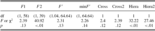
The dependent variable was the time needed to recognize a word (RT). RTs were measured from the beginning of the word's presentation. Stimuli were 60 words varying according to the factor A (fixed factor or treatment, two modalities: A1 vs. A2). Forty subjects were tested. Each item was presented once to each subject, and each subject was tested with all the items (2,400 measurements). Results obtained for each model are given in Table 2.
Results given by each model for the significance of the fixed factor
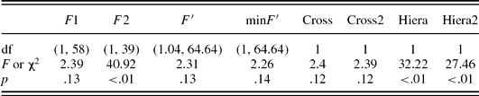
In this example, the conclusion in terms of significance of the effect derived from F′ is similar to that derived from the two cross-level models, from F1, and from minF′, whereas the conclusion derived from the hierarchical-level model is similar to that derived from F2. This similarity between models is due to the simplicity of the experimental design. Because we did not use any variable to describe the items in the hierarchical models, the variance of the items is conflated with the residual error at Level 1, as is the case with F2.
In conclusion, for this example, F1 + F2, F′, minF′ and the cross-level models reached the same and correct conclusion about the significant effect of the treatment. The benchmark study below shows however that in several cases the F1 + F2 procedure leads to an inflated Type I error.
BENCHMARKING THE TECHNIQUES
To compare the statistical accuracy of the different methods reviewed in this article and their robustness to a degradation of the data set, a benchmarking study is now presented. It is restricted to the simple design of Equation 2 and consists in estimating the real Type I error rate of each method. These benchmark results can be used for RTs as well as for other behavioral measurements following similar distribution properties.
Methodology
The simulation procedure consisted mainly of two parts: generating data sets and running the statistical analysis to evaluate Type I errors.
Generating data sets. We generated data sets according to the underlying model described in Equation 2, where both subjects and words are crossed random factors and where treatment (two modalities) is a fixed factor within subjects and between words. Standard deviation (σ) values (ms) were set to σS = 20, σTS = 17, and σW (T) = 29, and σe = 7. The recent literature argues that within a subject, RTs may be skewed, possibly ex-Gaussian; see, for example, Fagot, Dirk, Ghisletta, and de Ribaupierre (Reference Fagot, Dirk, Ghisletta and de Ribaupierre2009) for a review of the literature and several (real) data sets that support this assertion. For this reason, the last term was generated either as coming from a Gaussian distribution with the stated standard deviation (σe = 7) or as coming from an ex-Gaussian distribution with the variance shared in two equal parts between the exponential and the Gaussian component (roughly the proportion estimated in various conditions for the data analyzed in Fagot et al., Reference Fagot, Dirk, Ghisletta and de Ribaupierre2009). To estimate Type I error rates, we generated data with no mean difference between the two treatment values. We varied the total sample size by changing the number of subjects and words. We specified four total sample sizes: 10–10 (i.e., 10 subjects and 10 items), 15–15, 10–15, and 15–10. The results of the eight settings (two distributions [Gaussian or ex-Gaussian] by four sample sizes) are surprisingly highly similar. For the sake of text clarity, we present only two settings, which are those obtained for the 15–15 sample size, with the ex-Gaussian and with the Gaussian distribution.
We imitated MCAR missingness by randomly erasing values with probabilistic rules defined by two factors: the total amount of missing values in the data set (20%, 40%, or 60%), and their distribution across the two treatment conditions (balanced vs. unbalanced, respectively, half of the amount of missing values in each condition, vs. two-third and one-third). Both factors were fully crossed to define six missingness patterns (20 and 50–50, 20 and 33–67, 40 and 50–50, 40 and 33–67, 60 and 50–50, 60 and 33–67), the “experimental design” being completed with a no missing value control condition. We therefore used seven types of data sets for this investigation.
For F′, minF′, F1, F2, and F1 + F2, the incomplete data sets were first completed by applying three of the missing value replacement schemes presented in the Missing Values Section: grand mean, mean per condition, and means per subject and item. Conversely, because multilevel methods can be used with unbalanced designs, the incomplete data sets were directly tested with these methods.
Statistical analysis. For each of the 56 simulations (7 types of data sets × 8 statistical techniques), the procedure for generating data sets was repeated 10,000 times. The goal in repeating this procedure a large number of times is to obtain a more reliable estimate of the Type I error rate. The benchmarking procedure was programmed and run on S-Plus, and it produced an estimation of the true Type I error rate for each simulation, which is the expected or targeted rate of 0.05.
RESULTS
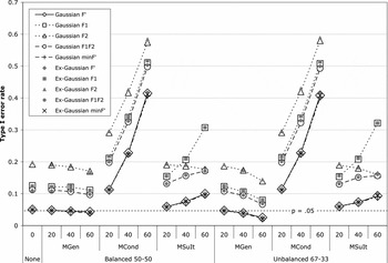
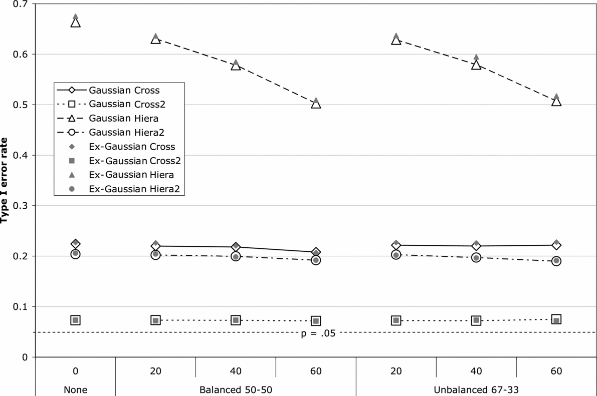
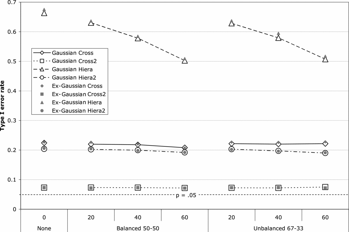
Figure 9 and Figure 10 show the percentages of null hypothesis rejection (the estimated Type I error rates) when the targeted decision criterion is α = 5% for the 15 items–15 subjects sample size. Figure 9 shows the results with F′, minF′, F1, F2, and F1 + F2. Figure 10 shows the results with the four multilevel models presented in Table 1: the cross-level model (Cross), the cross-level model with the additional interaction term T × S (Cross2), the hierarchical-level model (Hiera), and the hierarchical-level model with the additional interaction term T × S (Hiera2). The closer to the targeted 5% a method is, the more reliable it is.
Real Type I error rates depending on the F technique (F′, F1, F2, F1F2, minF′), the amount of missing values (0%, 20%, 40%, and 60%), the distribution of missing values across conditions (balanced, unbalanced), the replacement scheme applied to the data set (MGen, MCond, MSuIt), and the distribution type (Gaussian, ex-Gaussian). The percentages of missing values are indicated by 0, 20, 40, and 60; Balanced 50–50, the same number of missing values per condition; Unbalanced 67–33, two-thirds of the missing values in one condition, one-third in the other; MGen, the replacement of the missing values by the grand mean; MCond, replacement of the missing values in one condition by the mean for that condition; MSuIt, replacement of each missing value by a mean for this specific item and this specific subject; F′, quasi-F; F1, F test by subjects; F2, F test by items; F1F2, F1 + F2 procedure; minF′, lower bound for F′.

The real Type I error rates depending on the multilevel model type (Cross, Cross2, Hiera, Hiera2), the amount of missing values (0%, 20%, 40%, and 60%), the distribution of missing values across conditions (balanced, unbalanced), and the distribution type (Gaussian, ex-Gaussian). The percentages of missing values are indicated by 0, 20, 40, and 60; Balanced 50–50, the same amount of missing values per condition; Unbalanced 67–33, two-thirds of the missing values in one condition, one-third in the other; Cross, cross-level model; Cross2, cross-level model corresponding to F′; Hiera, hierarchical-level model corresponding to F1; Hiera2, hierarchical-level model Hiera augmented with the interaction term T × S.
DISCUSSION
A method is too conservative if it rejects fewer than 5% of the cases. It is too liberal if it rejects more than 5% of the cases. The estimated Type I error rate varies from simulation to simulation, depending on the different factors manipulated. For example, an estimated Type I error rate of 30% indicates that the corresponding method would yield a significant result in 30% of the cases, while 5% is expected. A correct method is neither conservative nor liberal, and will reject the null hypothesis 5 times out of 100 with the α criterion set to 0.05.
Accuracy of statistical techniques
We first note that the two simulated distributions (Gaussian and ex-Gaussian) give highly similar results. This might be attributable to the relative robustness of regression and ANOVA to skewed data, as long as the skewness is similar in all conditions (Miller, Reference Miller1997). Simulations reveal that the F′ method is the most reliable technique among those tested here. It gives the closest simulated Type I error to the expected 5% in the situation of no missing values. It has been said that F′ is too conservative, but this investigation clearly refutes such a point of view: F′ is accurate. In this study, minF′ gives almost the same results as F′. Comparatively, the F1 + F2 procedure used in psychology is always too liberal. This was expected from the theoretical aspects presented above. The MLM-crossed structure with the interaction term (Cross2) lies in between F′ and F1 + F2, offering a relatively good accuracy, although being more liberal than expected. It is however important to note that the other MLMs (Cross, Hiera, and Hiera2) are on the contrary too liberal. Because two hierarchical models are related to the model for F1 (see Table 1), and are therefore incomplete, this result was to be expected. Concerning the cross-level models, it shows the importance of modeling all terms, including the T × S interaction.
Impact of replacement scheme on the robustness of statistical techniques
These simulations show that the replacement scheme plays an important role for the accuracy of each technique. Replacing with a mean per condition will result in the poorest accuracy of Type I Error rate, followed by a replacement with means by subject and item. Replacing with the grand mean results in an excellent accuracy, which remains stable despite an augmentation of missing values, balanced as well as unbalanced. Note that accuracy refers here to the significance test, and the size effect will be affected by any replacement scheme. Combined with F′, the grand mean replacement scheme allows one to obtain the highest accuracy for the significance test. However, this conclusion is probably restricted to simple designs, such as the one we used for creating this benchmark. With two treatment factors, and with their interaction, we expect the precision, in the case of replacement by the grand mean, to deteriorate seriously, as explained in the Replacing the Missing Values by the Grand Mean Section. In such cases, the MLM approach will reveal its advantages, because it does not rely on any replacement scheme. Therefore, cross-level models with the interaction term (Cross2) can be considered as the best compromise between accuracy, performance, and ease of use. Moreover, in the case of missing values, one can argue that this method is somehow the EM algorithm version of F′. Because the underlying models for F′ and Cross2 are the same (see Table 1), using the EM algorithm with F′ or using Cross2 (with no replacement scheme) will give similar results.
Note that this benchmark is restricted to a situation where all methods apply. Multilevel models have the additional advantage of being applicable to a wider range of designs.
Finally, the results of this simulation are not restricted to chronographic data and can be applied to non-RT data, as long as the distribution is relatively close to Gaussian. We encourage researchers to use and report either F′ or cross-effect model results in all fields where they apply.
Summary and conclusion: F′ and cross-level multilevel models
In the case of no or few missing values, F′ appears to be the best statistical technique to use for its accuracy as a statistical test. This accuracy is preserved with an increasing number of missing values if missing values are replaced by the grand mean. However, the estimates provided for the experimental variables will become distorted, a drawback that is not found with MLM. Therefore, this simulation study reinforces the cross-level multilevel model as an excellent compromise: it is reasonably accurate, it does not rely on a missing value replacement scheme that can distort estimates and hamper accuracy, and it allows one to analyze more complex designs.
There are a few limitations to this simulation study. First, only one simple design (one fixed factor with two conditions) has been tested. Second, only MCAR types have been simulated. In the presence of a MAR type, some replacement schemes are expected to bias the results, as is expected with the averaging done in F1, F2, and thus F1 + F2 procedures. In this situation, MLM may even be more useful.
CONCLUSION
We have reviewed the different steps for processing RTs obtained through a repeated-measure design: filtering, missing values management, and choice of the statistical technique for significance testing. This tutorial has pointed out some common misconceptions and misuses of statistical techniques in the fields of scientific psychology. Resulting in statistical biases, these misconceptions and misuses can affect the results’ validity.
Although no universal recommendation can be made to counter these risks, F′ and cross-level models appear to fit better the experimental settings in our tests, especially in terms of statistical accuracy (Type I error rate).
Box (Reference Box and Wilkerson1979) said that “All models are wrong, but some are useful.” With today's huge computing abilities and the growing request to analyze properly each experiment, statisticians are stimulated to look for new models and approaches that will better capture data complexity. Because this process is not at its end, we hope that our article will encourage psychologists to use and investigate more efficient methods and models for analyzing their data.