1 Background

During the decomposition of the thermal protection system (TPS) of space vehicles during atmospheric entry, the gas injected into the boundary layer is a mixture of various species (Bhutta & Lewis Reference Bhutta and Lewis1992) resulting from the decomposition of the resin and the fibres. The properties of these species vary significantly from one to another, ranging from those that are overly lighter than air (such as H) to those that are much heavier (such as $\text{CO}_{2}$ or $\text{C}_{3}$). It is therefore important to understand how the transition dynamics vary when injecting gases with different characteristics.

During the 1960s and 1970s, several groups performed experimental campaigns with various gases injected through a porous surface in a slender cone in hypersonic conditions (Schneider Reference Schneider2010). An ablating TPS is typically formed of composite materials, where the resin and fibres decompose at different rates, thus having multiple porous-layer characteristics throughout the process – see Milos & Chen (Reference Milos and Chen2013). The mentioned experiments, with fixed porous-layer characteristics, therefore resemble a single instance within this process. However, many of them lacked the control of the test conditions that is necessary to come to a conclusion on the implications of such a composition modification. The most rigorous campaigns by Scott (Reference Scott1960), Marvin & Akin (Reference Marvin and Akin1970) and Stalmach et al. (Reference Stalmach, Bertin, Pope and McCloskey1971), observed that the injection of lighter gases (with a lower molar mass), such as He, moved transition upstream with respect to air injection. Heavier gases, such as $\text{CO}_{2}$ or $\text{CHClF}_{2}$, had the opposite effect. Marvin & Akin (Reference Marvin and Akin1970) developed a correlation weighing in also the molar mass of the injected gas, achieving a remarkable scaling of the experimental results. Stalmach et al. (Reference Stalmach, Bertin, Pope and McCloskey1971) then successfully tested this correlation by applying it to other injected gases, different from those employed by Marvin and Akin. These experimental efforts, however, where not followed by a corresponding theoretical analysis providing the causal link observed in the wind-tunnel tests.

More recently a joint experimental–numerical investigation (see Leyva et al. (Reference Leyva, Laurence, Beierholm, Hornung, Wagnild and Candler2009) or Jewell et al. (Reference Jewell, Wagnild, Leyva, Candler and Shepherd2013)) investigated the injection of $\text{CO}_{2}$ at the high temperatures featured in Caltech’s T5 reflected shock tunnel. In such instances, the three excited vibrational modes of the $\text{CO}_{2}$ molecule were seen to stabilize the flow and lead to a later transition. However, their research interest was focused on the mentioned vibrational-excitation transition delay, rather than on the link between the molar mass of the injected gas and the transition dynamics.

Another recent experimental–numerical study by Miró et al. (Reference Miró, Dehairs, Pinna, Gkolia, Masutti, Regert and Chazot2019) showed that discontinuous porous layers may advance transition, even when perturbations are locally stabilized above it, due to the excitation of otherwise stable perturbation frequencies. The authors also reported that the porous layer advanced transition differently in the blowing and non-blowing cases, suggesting a non-trivial coupling of the various phenomena. Surface injection was nevertheless seen to be destabilizing in all cases. Qualitatively similar results were obtained by Linn & Kloker (Reference Linn, Kloker and Glhan2008) with direct numerical simulations (DNS). However, the mentioned studies were restricted to a homogeneous gas composition, using air both as the injection and the wind-tunnel test gas.

There have also been efforts Lysenko et al. (Reference Lysenko, Gaponov, Smorodsky, Yermolaev and Kosinov2019) to explore the influence of the injection gas on transition. However, they were restricted to the supersonic regime, with Mach numbers much lower than those explored by Marvin & Akin (Reference Marvin and Akin1970) or Stalmach et al. (Reference Stalmach, Bertin, Pope and McCloskey1971), and too low to have second-mode instabilities dominate the transition process.

The present work addresses the main mechanisms by revisiting a configuration similar to that of Marvin and Akin, with a study based on linear stability theory. The following sections will separately elaborate on injection composition, surface porosity, transport modelling, and the injection profile and shocklet. The investigation is restricted to two-dimensional, second-mode waves, repeatedly reported to be the dominant instability leading to transition in noisy wind tunnels, such as the NASA Ames 3.5ft wind tunnel used in Marvin and Akin’s work – see Miró et al. (Reference Miró, Dehairs, Pinna, Gkolia, Masutti, Regert and Chazot2019) or Wagner (Reference Wagner2015).

2 Test conditions and gas modelling

Table 1.

Test conditions.

The test conditions employed for this investigation are summarized in table 1, which, for the sake of completeness, also includes the unit Reynolds number based on the boundary-layer-edge values ($Re_{1\,e}=\unicode[STIX]{x1D70C}_{e}u_{e}/\unicode[STIX]{x1D707}_{e}$) and the ratio between the isothermal wall and the recovery temperatures ($T_{w}/T_{adiab}$). The test gas is considered to be a non-reacting mixture of $\text{N}_{2}$, $\text{O}_{2}$, and an additional injected gas – He, Ne, Ar or $\text{CO}_{2}$. Due to the low test enthalpy, one can assume thermal equilibrium, with the thermal properties given by the rigid-rotor and harmonic-oscillator (RRHO) model – see Miró Miró et al. (Reference Miró Miró, Beyak, Pinna and Reed2019) and Miró Miró (Reference Miró Miró2020).

Table 2.

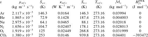
Species thermal and transport constants. Sutherland coefficients obtained from the CFD$++$ database (see Goldberg et al. Reference Goldberg, Peroomian, Chakravarthy and Sekar1997).

The Sutherland–Wilke (SW) model is employed to retrieve the mixture’s transport properties. The coefficients needed for the evaluation of Sutherland’s law for each species are obtained from the CFD$++$ database (see Goldberg et al. Reference Goldberg, Peroomian, Chakravarthy and Sekar1997), and are collected in table 2. The mixture transport properties are computed using the mixture rule proposed by Wilke (Reference Wilke1950). The diffusion fluxes are computed by employing the constant-Schmidt model with $Sc=0.7$.

The laminar base flow (denoted with an overbar: $\bar{q}$) is obtained from either solving the one-temperature multi-species boundary-layer (BL) or Navier–Stokes (NS) equations (see Miró Miró Reference Miró Miró2020) with frozen species chemical source terms ($\dot{\unicode[STIX]{x1D714}}_{s}=0$). The BL solutions are obtained with DEKAF (see Groot et al. (Reference Groot, Miró Miró, Beyak, Moyes, Pinna and Reed2018), Miró Miró et al. (Reference Miró Miró, Beyak, Mullen, Pinna and Reed2018a) or Ch. 7 in Miró Miró (Reference Miró Miró2020)), and the NS solutions with CFD$++$ (see Goldberg et al. Reference Goldberg, Peroomian, Chakravarthy and Sekar1997).

The subsequent spatial linear stability theory analyses (see Mack Reference Mack1984) on the perturbation amplitudes (denoted with a tilde: $\tilde{q}$) are performed with the VESTA toolkit (see Pinna Reference Pinna2013), exploiting the extended automatic derivation and implementation capabilities (see Pinna & Groot (Reference Pinna and Groot2014) and Ch. 8 in Miró Miró (Reference Miró Miró2020)). The base-line set of boundary conditions is the so-called homogeneous stability boundary condition (HSBC). It refers to a standard set of boundary conditions used in multi-species stability analyses (Miró Miró et al. Reference Miró Miró, Beyak, Pinna and Reed2019), featuring Dirichlet conditions ($\tilde{q}=0$) for all perturbation amplitudes, both at the free stream and wall boundaries, except for two: the species partial densities at the wall and the wall-normal velocity at the free stream. The former is accounted for by the linearized species wall-normal momentum conservation, and the latter by the linearized mixture continuity equation, evaluated at the corresponding boundary. Alternatively, one may employ the porous stability boundary condition at the wall (PSBC), obtained from generalizing the acoustic admittance treatment proposed by Gaponov (Reference Gaponov1978) and Fedorov et al. (Reference Fedorov, Malmuth, Rasheed and Hornung2001) to multi-species mixtures, as detailed in § 9.2 in Miró Miró (Reference Miró Miró2020). Similarly, one may also impose at the free stream the shock boundary condition, which is the result of linearizing the Rankine–Hugoniot relations across the shock, similarly to Stuckert & Reed (Reference Stuckert and Reed1994) or Pinna & Rambaud (Reference Pinna and Rambaud2013) – see Miró Miró (Reference Miró Miró2020). The integration of the $N$ factors for various frequencies of interest, employed in obtaining of the $N$-factor envelopes, was performed from their neutral point – see Arnal (Reference Arnal1993). Verification and validation comparisons for VESTA, DEKAF and CFD$++$ can be found in the work of Masutti et al. (Reference Masutti, Pinna, Gunaydinoglu, Sopek and Chazot2012), Grossir et al. (Reference Grossir, Pinna, Bonucci, Regert, Rambaud and Chazot2014), Martin et al. (Reference Martin, Grossir, Miró Miró, Le Quang and Chazot2019), Miró Miró et al. (Reference Miró Miró, Pinna, Beyak, Barbante and Reed2018b, Reference Miró Miró, Beyak, Pinna and Reed2019), Miró et al. (Reference Miró, Dehairs, Pinna, Gkolia, Masutti, Regert and Chazot2019) or Miró Miró (Reference Miró Miró2020).

Figure 1.

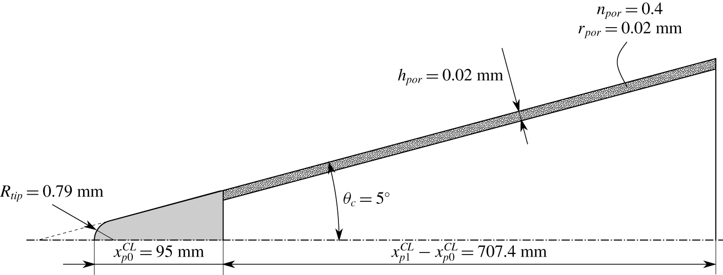
Sketch of the cone employed in the investigation, similar to Marvin & Akin (Reference Marvin and Akin1970).

Similarly to Marvin & Akin (Reference Marvin and Akin1970), the selected geometry is a 5-degree half-angle cone, with the physical characteristics summarized in figure 1. Both blunt and infinitely sharp tips are considered, with the former featuring a nose radius of 0.79 mm, equivalent to Marvin and Akin’s sharpest tested nose ($1/32~\text{in}$). When employing the PSBC, the porous layer is modelled with the characteristics reported by the authors ($n_{por}=0.4$ and $h_{por}=0.02~\text{mm}$) and assuming a pore radius of also $r_{por}=0.02~\text{mm}$. The pore radius is not reported, but Dr Marvin suggested, through private communication, that the pore size was sufficiently small, so as to have a uniformly blowing profile. It is therefore taken equal to $20~\unicode[STIX]{x03BC}\text{m}$, which, as seen in Miró Miró & Pinna (Reference Miró Miró and Pinna2018), leads to a minor modification of the stability characteristics when injecting air.

The theoretical characterization of this transpiring cone configuration has multiple aspects that must be considered:

1. (i) distinct composition of the injected gas;

2. (ii) transport modelling of a multi-species gas;

3. (iii) surface’s porous characteristics;

4. (iv) discontinuous blowing;

5. (v) nose bluntness;

6. (vi) injection shocklet.

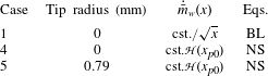
In order to effectively quantify their influence on the development of instabilities, a test matrix considering various geometries, injection profiles and equation systems is presented in table 3. It includes the Heaviside step function , which is 0 for $x<x_{0}$ and 1 for $x\geqslant x_{0}$, in order to model a discontinuous mass injection only through the porous section.

Figure 2.

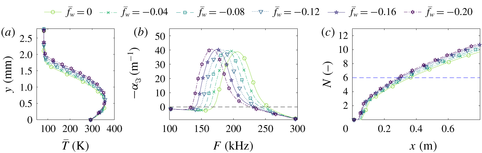
Base-flow temperature profiles at $x=508~\text{mm}$ (a), second-mode perturbation growth rates at $x=508~\text{mm}$ (b), and $N$-factor envelopes (c) for case 1 (see table 3) with air injection and various values of the self-similar injection parameter.

Table 3.

Test matrix. Suffixes ‘p’ and ‘s’ are added to the case identifier to denote the use of the PSBC and shock boundary condition, rather than the HSBC.

3 Distinct composition of the injected gas

First, the isolated effect of surface injection is explored by comparing the self-similar solution to the boundary-layer equations (case 1 in table 3), varying the blowing parameter $\bar{f}_{w}$ between 0 (no blowing) and $-0.2$ (positive blowing). Figure 2 displays the base-flow temperature profiles at $x=508~\text{mm}$ (a), together with the perturbation growth rates as a function of the perturbation frequency at that same location (b), and the envelope of the integrated $N$-factors as a function of the streamwise location (c). One can clearly observe how the larger boundary-layer thickness associated with a stronger blowing (figure 2a) leads to the well-known destabilization of the second mode and the decrease of the unstable frequency range (figure 2b) – see Johnson, Gronvall & Candler (Reference Johnson, Gronvall and Candler2009), Ghaffari et al. (Reference Ghaffari, Marxen, Iaccarino and Shaqfeh2010) or Miró Miró & Pinna (Reference Miró Miró and Pinna2018). This ultimately leads to the increase in the $N$-factor envelopes displayed in figure 2(c). The discontinuous blue line in figure 2(c) and all subsequent $N$-factor-envelope plots corresponds to an $N$ factor of 6, in the same range as that obtained by Miró et al. (Reference Miró, Dehairs, Pinna, Gkolia, Masutti, Regert and Chazot2019) in a similar outgassing investigation in the, also noisy, VKI-H3 wind tunnel. It is provided to give an estimation of where one could expect transition to occur under such conditions in an experiment.

The impact of injecting at the wall a gas different than the free stream one, air, (aspect (i) in § 2) is investigated by studying the self-similar solution to the multi-species non-reacting boundary-layer equations (case 1 in table 3). Such a solution is restricted to constant edge quantities (infinitely sharp cone) and blowing parameter $\bar{f}_{w}$ (implying an injection mass flow that scales like $x^{-1/2}$) (see Miró Miró (Reference Miró Miró2020) or White (Reference White1991)).

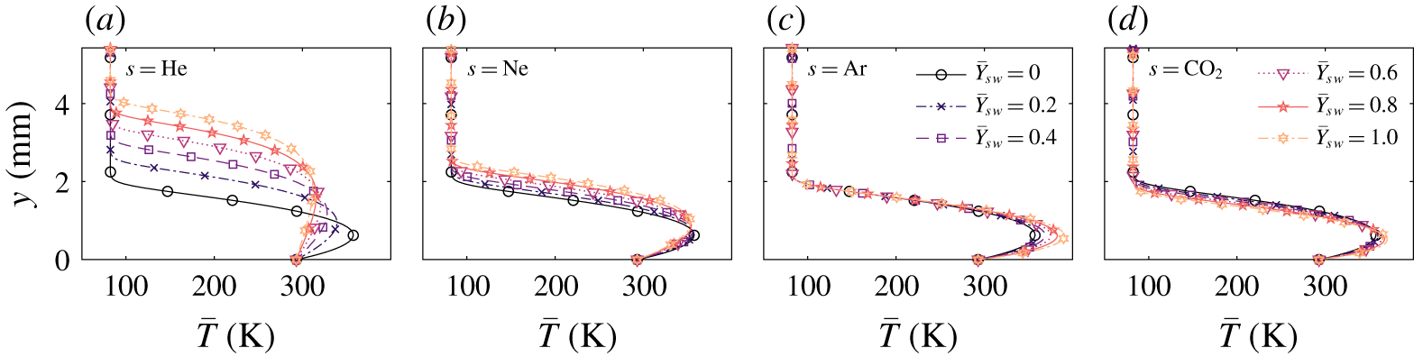
Figure 3 presents the temperature profile for six different wall concentrations of each of the four injected gases ($Y_{s\,w}$), ranging from 0 % to 100 % of the mixture. The blowing parameter $\bar{f}_{w}$ is kept constant for all cases and equal to $-0.2$, which corresponds to a positive injection velocity $v_{w}$. This implies that the injected mass flow remains constant for all the injection-gas compositions, similarly to what was done in the experiments by Marvin & Akin (Reference Marvin and Akin1970) or Stalmach et al. (Reference Stalmach, Bertin, Pope and McCloskey1971).

Figure 3.

Base-flow temperature profiles for case 1 (see table 3) at $x=508~\text{mm}$.

Figure 4.

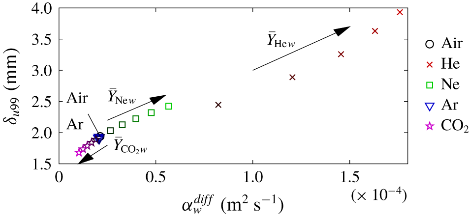
Boundary-layer thickness based on 99 % of the edge velocity, for each considered value of the thermal diffusivity at the wall. Different points for the same species correspond to 0 %, 20 %, 40 %, 60 %, 80 % and 100 % of it in the injected gas.

The comparison of the boundary-layer profiles in figure 3 suggests that the injection of gases with a higher thermal diffusivity than air (He and Ne) enlarge the boundary-layer thickness, whilst those with a similar one (Ar) do not modify it, and those with a lower one ($\text{CO}_{2}$) reduce it (see figure 4). The thermal diffusivity is defined as:

(3.1)$$\begin{eqnarray}\unicode[STIX]{x1D6FC}^{diff}=\frac{\unicode[STIX]{x1D705}}{\unicode[STIX]{x1D70C}c_{p}},\end{eqnarray}$$

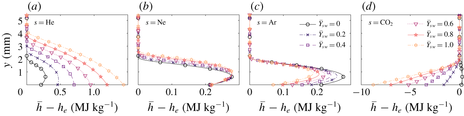
where $\unicode[STIX]{x1D705}$ is the thermal conductivity, $\unicode[STIX]{x1D70C}$ is the density and $c_{p}$ is the heat capacity. It is therefore a measure of how much energy is conducted away, with respect to the energy internally stored by a gas. For the particular problem at hand, a high thermal diffusivity implies that whatever enthalpy difference arises in the flow as a consequence of the injection of an external species, it is mostly conducted away from the wall. This increases accordingly the thermal boundary-layer thickness. Similarly, a low thermal diffusivity implies that such an enthalpy difference remains close to the surface. These traits are clearly distinguishable in the boundary-layer plots of the static-enthalpy difference for the various injection compositions, presented in figure 5. Note that the mentioned enthalpy difference may be due to a variation of the heat capacity (linked to the molar mass) or of the formation enthalpy (see table 2). A more thorough investigation on the influence of various gas properties on film cooling can be found in the work by Keller, Kloker & Olivier (Reference Keller, Kloker and Olivier2015).

Figure 5.

Base-flow profiles of the static-enthalpy difference for case 1 (see table 3).

Figure 6.

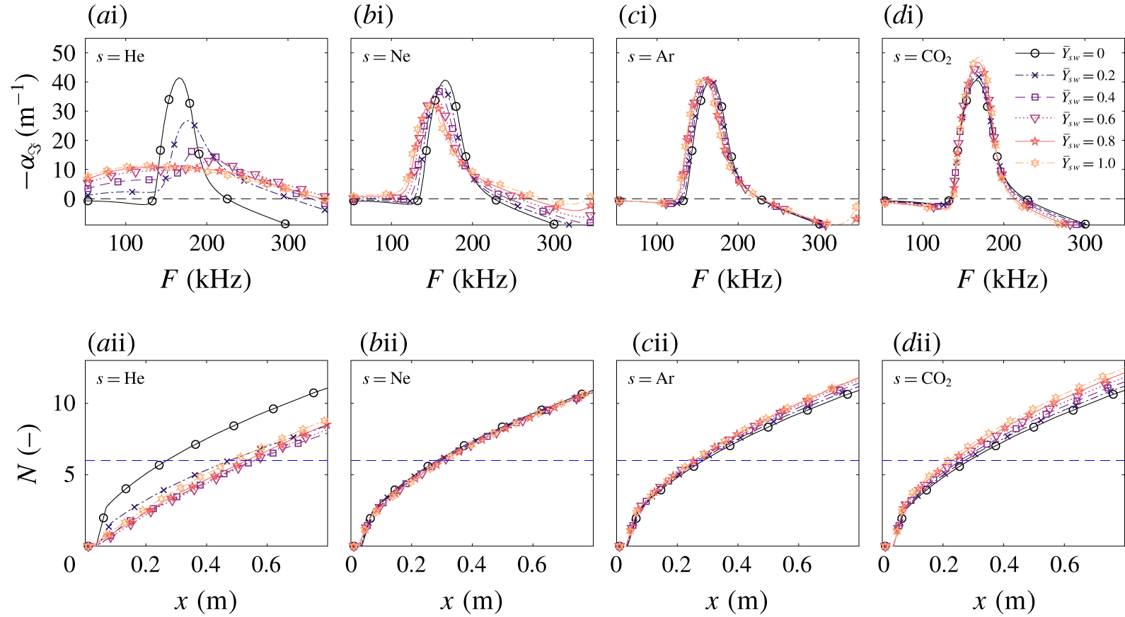
Second-mode perturbation growth rates at $x=508~\text{mm}$ (i) and $N$-factor envelopes (ii) for case 1 (see table 3).

Figure 6 displays the corresponding second-mode growth rates at $x=508~\text{mm}$ as a function of frequency (i) and the corresponding integrated $N$-factor envelopes (ii). The growth rates and $N$-factor envelopes display the opposite trend to what was obtained in the experiments. A higher concentration of lighter gases in the injected mixture leads to less unstable perturbations and lower $N$ factors, whilst a higher concentration of heavier gases has the opposite effect. Observing figure 6(a–bi), it is clear that, besides lowering the maximum amplification rate, a higher helium or neon concentration at the wall also increases the range of unstable frequencies. One could therefore expect the integration of the $N$ factors to lead to a sooner transition-onset prediction similar to that observed in the experiments. Figure 6(a–dii) indeed displays the result of the competing effect of the decrease in the maximum amplification rate (delaying transition) and the widening of the unstable frequency range (advancing transition) for the lighter-gas cases (figure 6a–bii). The variation of the wall concentration of neon (figure 6bii) displays a balance of these two effects, which ultimately leads to a negligible change of the predicted transition-onset location. The $N$-factor envelopes for scenarios injecting heavier gases (figure 6c–dii) present the same trend observed in the growth rates in figure 6(c–di): a higher concentration of heavier gases ultimately leads to a sooner predicted transition onset.

One could speculate that the dominant instability, when increasing the concentration of He, is no longer a second mode (see figure 6ai). However, varying spanwise-wavenumber analyses discarded this possibility, ensuring that second-mode waves remained dominant.

Overall, the observed trend does not coincide with the experimental findings reported by Marvin & Akin (Reference Marvin and Akin1970), Scott (Reference Scott1960) and Stalmach et al. (Reference Stalmach, Bertin, Pope and McCloskey1971), being actually opposite to them. This suggests that the advancement/delay of the transition front that they experienced when injecting lighter/heavier gases was not exclusively due to the modification of the injection composition. On the contrary, this effect delays transition for lighter gases and advances it for heavier ones.

4 Transport modelling of a multi-species gas

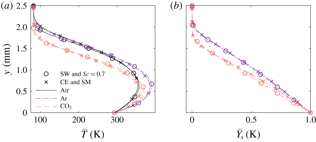
The dependency of the observed trends on the thermophysical gas modelling (aspect (ii) in § 2) is evaluated by revisiting case 1, yet modifying the transport and the diffusion models for injection mixtures with 100 % of either air, argon or $\text{CO}_{2}$. Two different sets of models are compared: SW and a constant $Sc=0.7$ (like in the rest of the article), or Chapman–Enskog (CE) transport and Stefan–Maxwell (SM) diffusion (see Miró Miró et al. Reference Miró Miró, Beyak, Pinna and Reed2019). For the latter combination, the necessary collisional data are obtained from fitting a polynomial-logarithmic expression to the data in Wright et al. (Reference Wright, Bose, Palmer and Levin2005), Wright, Hwang & Schwenke (Reference Wright, Hwang and Schwenke2007). The corresponding curve-fit coefficients are collected in Miró Miró (Reference Miró Miró2020).

One must note that for the considered temperature range (70–400 K), these curve fits are mostly an extrapolation from the original data points. Therefore, the CE and SM models do not offer the higher fidelity, with respect to the SW and the constant $Sc=0.7$ models, as for high-temperature scenarios – see Miró Miró et al. (Reference Miró Miró, Beyak, Pinna and Reed2019). The comparison displayed in this section thus serves as a metric of the sensitivity of the predictions to modelling variations, and it is not an evaluation of the accuracy achievable with the employed models.

Figure 7.

Base-flow profiles for case 1 (see table 3) at $x=508~\text{mm}$ for two sets of models and various injection gases.

Figure 8.

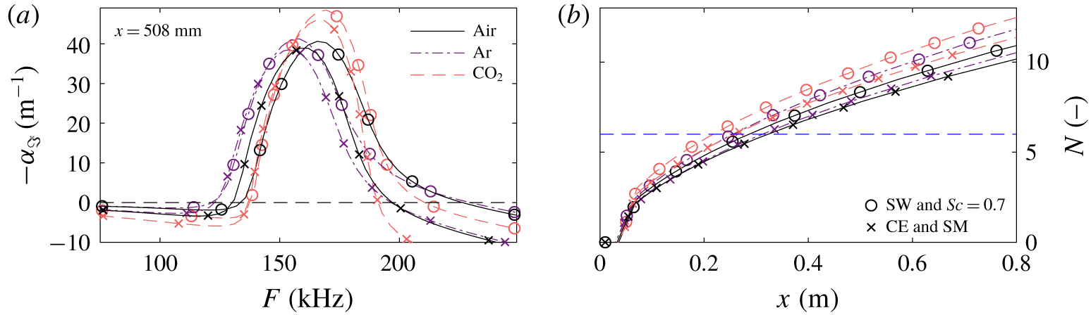
Second-mode perturbation growth rates at $x=508~\text{mm}$ (a) and $N$-factor envelopes (b) for case 1 (see table 3) for two sets of models and various injection gases.

The base-flow profiles obtained with the two sets of models are presented in figure 7. The use of one or another set is seen to have a minor impact on the boundary-layer profiles. It is, however, noteworthy that the CE and SM models predict a stronger cooling and a larger thermal boundary-layer thickness than the SW and constant $Sc=0.7$ models (figure 7a). This same trend was reported in Miró Miró et al. (Reference Miró Miró, Beyak, Pinna and Reed2019) when comparing the CE and the Blottner–Eucken–Wilke (BEW) transport models.

Figure 8 displays the second-mode growth rates as a function of frequency at $x=508~\text{mm}$ (a) and the integrated $N$-factor envelopes (b) for the laminar base flow presented in figure 7. The CE and SM models foresee lower growth rates and $N$ factors than the SW and the constant $Sc=0.7$ models. This shift, however, is consistent across all mixtures. Blowing heavier gases destabilizes the flow, regardless of the transport and diffusion models employed.

It is thus clear that the observed destabilizing effect of injecting heavier gases is independent of the transport and diffusion model.

5 Porosity, discontinuous blowing, nose bluntness, and injection shocklet

Figure 9.

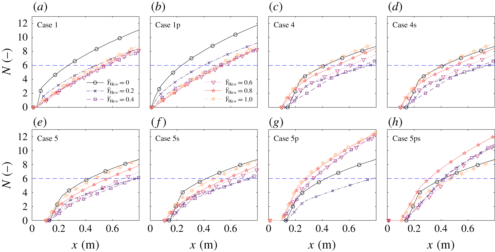
Second-mode $N$-factor envelopes for various cases (see table 3) and He concentrations in the injected mixture.

Aspects (iii)–(vi) of those listed at the end of § 2 are examined in figure 9. The influence of porosity (iii) on a continuously blowing configuration (case 1) is seen to be negligible, since the $N$-factor envelopes for cases 1 and 1p (the suffix p denotes the PSBC) do not present significant differences (figures 9a and 9b respectively). However, the combination of the porous boundary condition with a discontinuous blowing can lead to unexpected outcomes because of the competing stabilizing and destabilizing effects – see Miró et al. (Reference Miró, Dehairs, Pinna, Gkolia, Masutti, Regert and Chazot2019).

The base flows in cases 4 and 5 are obtained from solving the NS rather than the BL equations, and feature a step-wise injection profile. The mass flux is constant ($\dot{\bar{m}}_{w}=7.35~\text{g}~\text{s}^{-1}~\text{m}^{-2}$) in the injection region (see figure 1). The difference between cases 4 and 5 lies in the tip of the cone: infinitely sharp for case 4 and blunt with a nose radius of 0.79 mm for case 5 (the same as in Marvin and Akin’s sharpest cone – see figure 1).

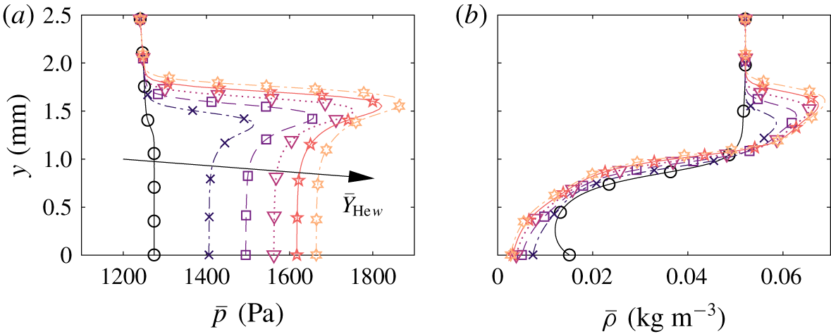
A differentiating feature of the cases with a discontinuous mass injection (cases 4 and 5) with respect to case 1 is the appearance of a density gradient at the injection point, translating into a shocklet even if the density gradient is locally negative (see figure 10). The shocklet gradually dissipates as it advances downstream, and is ultimately absorbed by the main shock. The intensity of the shocklet is proportional to the helium concentration in the injected mixture, being almost undetectable when injecting pure air. It is therefore hereinafter referred to as a ‘concentration shocklet’.

The existence of this concentration shocklet raises a question regarding its modelling in stability analyses. Since it is a weak shocklet, one could simply keep it within the computational wall-normal domain, and impose a Dirichlet condition at $y_{max}$, as done in all the other analyses in this article. Another possibility is to restrict the computational domain to the region within the concentration shocklet, and employ the shock perturbation boundary condition on it. The downside to the latter approach is that it neglects the perturbation propagation after the concentration shocklet ($y>y_{shock}$), since the shock boundary condition assumes $\tilde{q}=0$ in that wall-normal range. However, the advantage is that it does allow for shock oscillation and a coupling with the instabilities. The shock-boundary-condition approach is denoted with the suffix s on the case identifier (for instance case 5 and 5s).

Figure 10.

Pressure (a) and density (b) profiles at $x=0.1~\text{m}$ showing the injection shocklet for case 5 (see table 3) and for various helium concentrations in the injected mixture.

The discontinuous injection of mass through the surface leads to substantially different $N$-factor envelopes. Cases 4 and 5 (figure 9c and e) present lower $N$ factors for the 0 % He-injection case than cases 1 and 1p. However, more significantly, they also present a much larger advancement of the transition front than cases 1 and 1p when increasing $Y_{\text{He}\,w}$, after the initial delay. This advancement is large enough to have the $N$-factor curve for 100 % He almost coincide with that of 0 % He. This trend is also almost independent of the strategy employed to deal with the concentration shocklet, since cases 4s and 5s (figure 9d and f) present almost identical $N$-factor envelopes to cases 4 and 5 (figure 9c and e). Moreover, the similarity between the predictions of cases 4 and 5 suggests that the cone’s bluntness ($R_{tip}=0.79~\text{mm}$) is not sufficient to modify the dynamics of instability development.

The complete reversal of the trend observed for continuously blowing scenarios with the HSBC, occurs when one considers simultaneously a discontinuous blowing and a PSBC (case 5p in figure 9g). This is similar to what was observed in Miró et al. (Reference Miró, Dehairs, Pinna, Gkolia, Masutti, Regert and Chazot2019), where the porous layer was seen to affect differently the development of instabilities with and without mass injection.

It is interesting, however, to observe that case 5ps in figure 9(h) does not predict such a reversal. Case 5ps simultaneously employs the shock boundary condition, truncating the domain at the concentration shocklet, and the porous (PSBC). A possible explanation for this can be given based on the thermoacoustic interpretation of the second mode recently formulated by Kuehl (Reference Kuehl2018). According to it, the second mode must be interpreted as an acoustic wave confined by the thermoacoustic impedance that is the large density gradient at the top of the boundary layer. The concentration shocklet arising after the injection region (see figure 10) is indeed one of such thermoacoustic impedances.

This impedance is considered by case 5p but not by case 5ps. The use of the shock boundary condition (case 5ps) imposes a different impedance, coming from the linearization of the Rankine–Hugoniot relations. The thermoacoustic coupling of the porous wall and the concentration shocklet appears to increase the growth rates after the injection for lighter gases, and ultimately shifts the corresponding $N$-factor curves vertically.

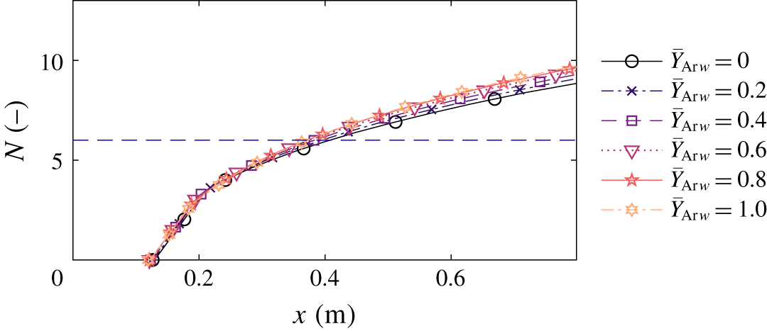
Case 5p (discontinuous blowing with a blunt nose and with the PSBC) is also investigated for argon injection, in order to assess whether it is indeed the appropriate modelling strategy or not. The mass flow per unit surface through the porous section is also kept constant and equal to $\dot{\bar{m}}_{w}=7.35~\text{g}~\text{s}^{-1}~\text{m}^{-2}$ in the injection streamwise region. The corresponding $N$-factor envelopes for six different argon concentrations are displayed in figure 11. Similarly to what was observed experimentally by Marvin & Akin (Reference Marvin and Akin1970), the injection of argon instead of air almost leaves the predicted transition-onset location unchanged. There appears to be a minor advancement associated with higher argon concentrations in the injected mixture. However, this subtle difference could have been inappreciable in the experiments due to the measurement uncertainty.

Figure 11.

Second-mode $N$-factor envelopes for various case 5p in table 3 with argon injection.