2 Problem layout

We assume the classic vortex-sheet profile of KH instability (Batchelor Reference Batchelor2000; Drazin & Reid Reference Drazin and Reid2004):

(2.1a,b ) $$\begin{eqnarray}\displaystyle \bar{u}(z)=\left\{\begin{array}{@{}ll@{}}U\quad & z>0\\ -U\quad & z<0\end{array}\right.\quad \text{and}\quad \bar{\unicode[STIX]{x1D70C}}(z)=\left\{\begin{array}{@{}ll@{}}\unicode[STIX]{x1D70C}_{1}\quad & z>0,\\ \unicode[STIX]{x1D70C}_{2}\quad & z<0,\end{array}\right. & & \displaystyle\end{eqnarray}$$

where $\bar{u}$ and $\bar{\unicode[STIX]{x1D70C}}$ , respectively, denote the streamwise ( $x$ ) background velocity and background density (with $\unicode[STIX]{x1D70C}_{2}\geqslant \unicode[STIX]{x1D70C}_{1}$ ), and $z$ points vertically upwards. The vortex sheet is perturbed by an infinitesimal sinusoidal disturbance of the form $\exp [\text{i}(kx/\unicode[STIX]{x1D6FD}+ly-\unicode[STIX]{x1D6FA}_{\unicode[STIX]{x1D6FD}}t)]$ , where $k/\unicode[STIX]{x1D6FD}\in \mathbb{R}^{+}$ and $l\in \mathbb{R}^{+}$ are, respectively, the streamwise and spanwise wavenumbers, and $\unicode[STIX]{x1D6FA}_{\unicode[STIX]{x1D6FD}}\in \mathbb{C}$ is the frequency.

Figure 2.

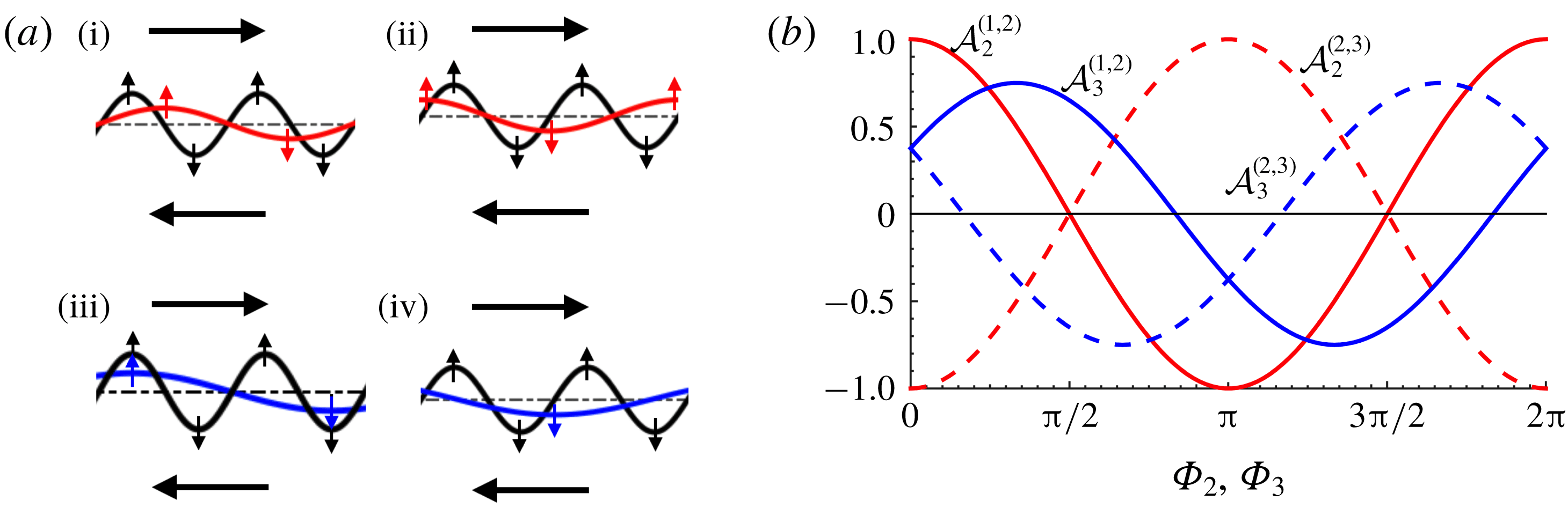
(a) Schematic showing the first two wavelengths of the primary mode of a KH instability, and its first and second subharmonic modes for different phase shifts. The horizontal (vertical) arrows represent horizontal (vertical) velocity. First subharmonic ( $\unicode[STIX]{x1D6FD}=2$ ) for (i) $\unicode[STIX]{x1D6F7}_{2}=0$ (maximum asymmetry) and (ii) $\unicode[STIX]{x1D6F7}_{2}=\unicode[STIX]{x03C0}/2$ (minimum asymmetry). Second subharmonic ( $\unicode[STIX]{x1D6FD}=3$ ) for (iii) $\unicode[STIX]{x1D6F7}_{3}=\unicode[STIX]{x03C0}/3$ (maximum asymmetry) and (iv) $\unicode[STIX]{x1D6F7}_{3}=5\unicode[STIX]{x03C0}/6$ (minimum asymmetry). (b) Variation of sample asymmetries with phase shifts. Three consecutive wavelengths of the primary wave are considered. Red and blue colour, respectively, indicate asymmetry induced by the first and the second subharmonics. While solid lines denote asymmetry between the first and the second primary waves, dashed lines denote the same between the second and the third. The coefficient $4\unicode[STIX]{x1D6FD}\unicode[STIX]{x1D6FE}_{\unicode[STIX]{x1D6FD}}\hat{\unicode[STIX]{x1D702}}_{\unicode[STIX]{x1D6FD}}(0)/(k\unicode[STIX]{x1D6FE}_{1}\hat{\unicode[STIX]{x1D702}}_{1}(0))$ of ${\mathcal{A}}_{\unicode[STIX]{x1D6FD}}^{(m,m+1)}$ is assumed to be $1$ in each case.

Although the velocities at the interface are not defined, they can be calculated by taking the arithmetic mean of the velocities just above and below the interface. The perturbation vertical velocity at the interface is obtained by exploiting the linearized kinematic condition at the interface with $\bar{u}=0$ :

(2.2) $$\begin{eqnarray}\displaystyle & \displaystyle \frac{\unicode[STIX]{x2202}\unicode[STIX]{x1D702}_{\unicode[STIX]{x1D6FD}}}{\unicode[STIX]{x2202}t}+\bar{u}\frac{\unicode[STIX]{x2202}\unicode[STIX]{x1D702}_{\unicode[STIX]{x1D6FD}}}{\unicode[STIX]{x2202}x}=w_{\unicode[STIX]{x1D6FD}}=-\text{i}\unicode[STIX]{x1D6FA}_{\unicode[STIX]{x1D6FD}}\unicode[STIX]{x1D702}_{\unicode[STIX]{x1D6FD}}, & \displaystyle\end{eqnarray}$$

where $\unicode[STIX]{x1D702}_{\unicode[STIX]{x1D6FD}}$ denotes the interface elevation. This shows that $w_{\unicode[STIX]{x1D6FD}}$ has the same phase as $\unicode[STIX]{x1D702}_{\unicode[STIX]{x1D6FD}}$ provided $\unicode[STIX]{x1D6FA}_{\unicode[STIX]{x1D6FD}}$ is purely imaginary (unstable flow with zero phase speed).

The classic dispersion relation for KH instability under the Boussinesq approximation yields (Drazin & Reid Reference Drazin and Reid2004),

(2.3) $$\begin{eqnarray}\displaystyle & \displaystyle \unicode[STIX]{x1D6FA}_{\unicode[STIX]{x1D6FD}}\equiv \text{i}\unicode[STIX]{x1D6FE}_{\unicode[STIX]{x1D6FD}}=\pm \text{i}\sqrt{\left(U\frac{k}{\unicode[STIX]{x1D6FD}}\right)^{2}-Atg\tilde{k}}, & \displaystyle\end{eqnarray}$$

where $\unicode[STIX]{x1D6FE}_{\unicode[STIX]{x1D6FD}}$ is the growth rate, $\tilde{k}=\sqrt{(k/\unicode[STIX]{x1D6FD})^{2}+l^{2}}$ , $At\equiv (\unicode[STIX]{x1D70C}_{2}-\unicode[STIX]{x1D70C}_{1})/(\unicode[STIX]{x1D70C}_{1}+\unicode[STIX]{x1D70C}_{2})$ is the Atwood number and $g$ is gravitational acceleration. Equation (2.3) shows that for instability, $\unicode[STIX]{x1D6FA}_{\unicode[STIX]{x1D6FD}}$ is purely imaginary; hence, $w_{\unicode[STIX]{x1D6FD}}$ and $\unicode[STIX]{x1D702}_{\unicode[STIX]{x1D6FD}}$ have the same phase. This fact has a very important consequence in vortex merging, which will be elaborated in the following discussions.

For now we restrict ourselves to 2-D flows ( $x{-}z$ ) with polychromatic waves in the streamwise direction (note that now $l=0$ ); $k$ is the wavenumber of the primary mode and $\unicode[STIX]{x1D6FD}$ is its $(\unicode[STIX]{x1D6FD}-1)$ th subharmonic; $\unicode[STIX]{x1D6FD}=2,3,\ldots$  . Equation (2.3) shows that the growth rate $\unicode[STIX]{x1D6FE}_{\unicode[STIX]{x1D6FD}}$ is inversely proportional to $\unicode[STIX]{x1D6FD}$ . Hence, the primary mode has the fastest growth rate, and the higher the subharmonic, the weaker is its growth rate. We first consider an interface perturbed by a dichromatic disturbance which has modes $k$ and $k/\unicode[STIX]{x1D6FD}$ . Hence, the initial disturbance has the form

(2.4) $$\begin{eqnarray}\unicode[STIX]{x1D702}(x,0)=\hat{\unicode[STIX]{x1D702}}_{1}(0)\sin (kx)+\hat{\unicode[STIX]{x1D702}}_{\unicode[STIX]{x1D6FD}}(0)\sin (kx/\unicode[STIX]{x1D6FD}+\unicode[STIX]{x1D6F7}_{\unicode[STIX]{x1D6FD}}),\end{eqnarray}$$

where $\unicode[STIX]{x1D6F7}_{\unicode[STIX]{x1D6FD}}\in [0,2\unicode[STIX]{x03C0})$ denotes the phase difference between the primary and the subharmonic modes. This initial disturbance for a short time would evolve as

(2.5) $$\begin{eqnarray}\unicode[STIX]{x1D702}(x,t)=\hat{\unicode[STIX]{x1D702}}_{1}(0)\text{e}^{\unicode[STIX]{x1D6FE}_{1}t}\sin (kx)+\hat{\unicode[STIX]{x1D702}}_{\unicode[STIX]{x1D6FD}}(0)\text{e}^{\unicode[STIX]{x1D6FE}_{\unicode[STIX]{x1D6FD}}t}\sin (kx/\unicode[STIX]{x1D6FD}+\unicode[STIX]{x1D6F7}_{\unicode[STIX]{x1D6FD}}),\end{eqnarray}$$

provided $t$ is small enough so that linearity of the system is respected.

2.1 Quantifying vortex merging from initial asymmetry

The physical mechanism behind vortex pairing is explained in figure 2. In figure 2(ai), the first subharmonic mode (in red) tends to oppositely displace consecutive wavelengths of the primary mode (in black); the first wavelength (which gives rise to the first KH billow) moves upwards while the second (which gives rise to the second KH billow) moves downwards. The horizontal velocity shear advects the centre of the billows towards each other, leading to pairing. If no asymmetry is introduced by the subharmonic mode, there would not be any pairing; see figure 2(aii). The only difference between figure 2(ai) and figure 2(aii) is the phase shift, $\unicode[STIX]{x1D6F7}_{2}$ . In a very similar manner, the second subharmonic induces pairing in figure 2(aiii) but does not in figure 2(aiv). The basis of the above argument is the fact that the interface elevation of any given mode and the corresponding vertical velocity are in phase.

Since asymmetry induced by the $w$ velocity in two neighbouring wavelengths of the primary mode leads to merging, we propose a quantitative measure that captures this effect. We consider two consecutive wavelengths of the primary mode and find the integral of the $w$ velocity in each of them. The integrated $w$ velocity due to the primary mode will always cancel out, but that due to the subharmonic mode can remain. We define a quantity ${\mathcal{A}}$ that measures the strength of the subharmonic-mode-induced asymmetry with respect to the $w$ velocity amplitude of the primary mode. Mathematically we write it as follows:

(2.6) $$\begin{eqnarray}\displaystyle \displaystyle {\mathcal{A}}_{\unicode[STIX]{x1D6FD}}^{(m,m+1)}(t) & = & \displaystyle \frac{{\hat{w}}_{\unicode[STIX]{x1D6FD}}(t)}{{\hat{w}}_{1}(t)}\left[\int _{2(m-1)\unicode[STIX]{x03C0}/k}^{2m\unicode[STIX]{x03C0}/k}\sin \left(\frac{k}{\unicode[STIX]{x1D6FD}}x+\unicode[STIX]{x1D6F7}_{\unicode[STIX]{x1D6FD}}\right)\,\text{d}x-\int _{2m\unicode[STIX]{x03C0}/k}^{2(m+1)\unicode[STIX]{x03C0}/k}\sin \left(\frac{k}{\unicode[STIX]{x1D6FD}}x+\unicode[STIX]{x1D6F7}_{\unicode[STIX]{x1D6FD}}\right)\,\text{d}x\right]\nonumber\\ \displaystyle & = & \displaystyle -\frac{4\unicode[STIX]{x1D6FD}}{k}\frac{\unicode[STIX]{x1D6FE}_{\unicode[STIX]{x1D6FD}}\hat{\unicode[STIX]{x1D702}}_{\unicode[STIX]{x1D6FD}}(0)}{\unicode[STIX]{x1D6FE}_{1}\hat{\unicode[STIX]{x1D702}}_{1}(0)}\text{e}^{(\unicode[STIX]{x1D6FE}_{\unicode[STIX]{x1D6FD}}-\unicode[STIX]{x1D6FE}_{1})t}\sin ^{2}\left(\frac{\unicode[STIX]{x03C0}}{\unicode[STIX]{x1D6FD}}\right)\cos \left(\frac{2m\unicode[STIX]{x03C0}}{\unicode[STIX]{x1D6FD}}+\unicode[STIX]{x1D6F7}_{\unicode[STIX]{x1D6FD}}\right).\end{eqnarray}$$

The prefix ‘ $m,m+1$ ’ of ${\mathcal{A}}_{\unicode[STIX]{x1D6FD}}$ signifies that we are comparing the $m$ th wavelength with the $(m+1)$ th wavelength of the primary mode, where the asymmetry is induced by the $(\unicode[STIX]{x1D6FD}-1)$ th subharmonic. The asymmetry is predicted after time $t$ based on linear theory. Unless otherwise stated, we will evaluate the asymmetry at the initial time ( $t=0$ ). ${\mathcal{A}}_{\unicode[STIX]{x1D6FD}}^{(m,m+1)}>0$ implies that two nearby vortices move towards each other and undergo merging; the higher the magnitude, the quicker is the merging. Likewise, ${\mathcal{A}}_{\unicode[STIX]{x1D6FD}}^{(m,m+1)}<0$ implies that the two neighbouring vortices move away from each other. We also note that, although the asymmetry seems directly proportional to $\unicode[STIX]{x1D6FD}$ in (2.6), it is actually the opposite, which can be quickly verified from the terms $\unicode[STIX]{x1D6FE}_{\unicode[STIX]{x1D6FD}}/\unicode[STIX]{x1D6FE}_{1}$ and $\sin ^{2}(\unicode[STIX]{x03C0}/\unicode[STIX]{x1D6FD})$ .

The phases leading to the maximum and minimum magnitudes of ${\mathcal{A}}_{\unicode[STIX]{x1D6FD}}^{(m,m+1)}$ are

(2.7) $$\begin{eqnarray}\displaystyle \left.\begin{array}{@{}c@{}}\displaystyle \unicode[STIX]{x1D6F7}_{\unicode[STIX]{x1D6FD}}^{max}=m\unicode[STIX]{x03C0}\left(1-\frac{2}{\unicode[STIX]{x1D6FD}}\right)\quad \text{and}\quad \unicode[STIX]{x03C0}\left[1+m\left(1-\frac{2}{\unicode[STIX]{x1D6FD}}\right)\right],\\[12.0pt] \displaystyle \unicode[STIX]{x1D6F7}_{\unicode[STIX]{x1D6FD}}^{min}=\unicode[STIX]{x03C0}\left[\frac{1}{2}+m\left(1-\frac{2}{\unicode[STIX]{x1D6FD}}\right)\right]\quad \text{and}\quad \unicode[STIX]{x03C0}\left[\frac{3}{2}+m\left(1-\frac{2}{\unicode[STIX]{x1D6FD}}\right)\right].\end{array}\right\} & & \displaystyle\end{eqnarray}$$

Figure 2(b) shows the variation of ${\mathcal{A}}_{\unicode[STIX]{x1D6FD}}^{(m,m+1)}$ with phase shift. The asymmetries induced by the first and the second subharmonics have been separately computed. An important observation is that asymmetries between two different subharmonics can largely add up or can largely cancel out. To elaborate this point further, let us assume that the interface is initially perturbed with the primary disturbance and its first and second subharmonics:

(2.8) $$\begin{eqnarray}\displaystyle & \displaystyle \unicode[STIX]{x1D702}(x,0)=\hat{\unicode[STIX]{x1D702}}_{1}(0)\sin \left(kx\right)+\hat{\unicode[STIX]{x1D702}}_{2}(0)\sin \left(\frac{k}{2}x+\unicode[STIX]{x1D6F7}_{2}\right)+\hat{\unicode[STIX]{x1D702}}_{3}(0)\sin \left(\frac{k}{3}x+\unicode[STIX]{x1D6F7}_{3}\right). & \displaystyle\end{eqnarray}$$

Here, six consecutive wavelengths of the primary wavelength need to be considered for observing the merging pattern (which would repeat after every six wavelengths). We do not consider any higher subharmonics ( $\unicode[STIX]{x1D6FD}>3$ ) since the growth rates of these modes fall rapidly and are therefore of little consequence. We define the total asymmetry at $t=0$ between two consecutive wavelengths (of the primary mode) as

(2.9) $$\begin{eqnarray}\displaystyle {\mathcal{A}}_{total}^{(m,m+1)}={\mathcal{A}}_{2}^{(m,m+1)}+{\mathcal{A}}_{3}^{(m,m+1)}. & & \displaystyle\end{eqnarray}$$

2.2 Predicting vortex merging from initial asymmetry

Depending on the phases $\unicode[STIX]{x1D6F7}_{2}$ and $\unicode[STIX]{x1D6F7}_{3}$ , the asymmetries induced by these two subharmonics may largely add up or may largely cancel out. For simplicity, we restrict to unstratified shear flows ( $At=0$ ). We span the entire $\unicode[STIX]{x1D6F7}_{2}{-}\unicode[STIX]{x1D6F7}_{3}$ space to see what combinations of these phase shifts lead to high or low asymmetry. We also limit our analysis to initial amplitudes satisfying

(2.10) $$\begin{eqnarray}\displaystyle (\hat{\unicode[STIX]{x1D702}}_{2}(0)/\hat{\unicode[STIX]{x1D702}}_{1}(0))^{2}+(\hat{\unicode[STIX]{x1D702}}_{3}(0)/\hat{\unicode[STIX]{x1D702}}_{1}(0))^{2}=2. & & \displaystyle\end{eqnarray}$$

In this respect three cases are considered:

1. (i) Case C1: $\hat{\unicode[STIX]{x1D702}}_{2}(0)/\hat{\unicode[STIX]{x1D702}}_{1}(0)=1.41$ and $\hat{\unicode[STIX]{x1D702}}_{3}(0)/\hat{\unicode[STIX]{x1D702}}_{1}(0)=0.11$ ,

2. (ii) Case C2: $\hat{\unicode[STIX]{x1D702}}_{2}(0)/\hat{\unicode[STIX]{x1D702}}_{1}(0)=1$ and $\hat{\unicode[STIX]{x1D702}}_{3}(0)/\hat{\unicode[STIX]{x1D702}}_{1}(0)=1$ ,

3. (iii) Case C3: $\hat{\unicode[STIX]{x1D702}}_{2}(0)/\hat{\unicode[STIX]{x1D702}}_{1}(0)=0.11$ and $\hat{\unicode[STIX]{x1D702}}_{3}(0)/\hat{\unicode[STIX]{x1D702}}_{1}(0)=1.41$ .

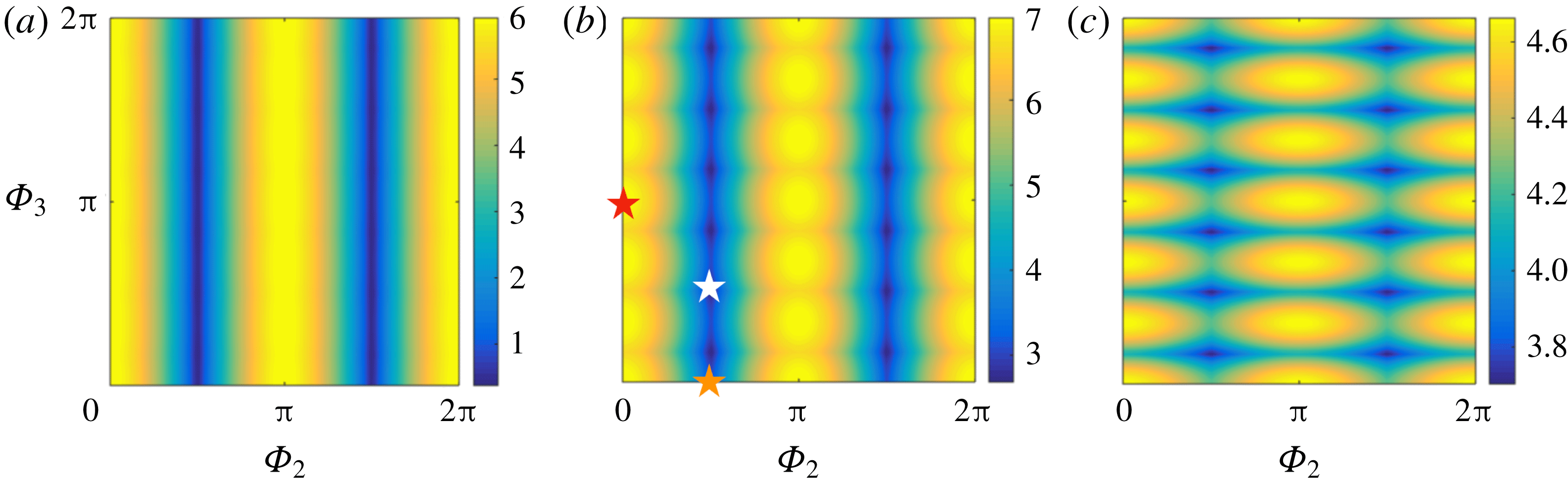
Furthermore, since asymmetry depends on the wavelength-pair ‘ $m,m+1$ ’, we consider the maximum absolute asymmetry – i.e. $\max \left(\left|A_{total}\right|\right)$ among all ‘ $m,m+1$ ’ pairs – and plot it in figure 3. We observe that when the first subharmonic is very strong (figure 3 a), $\max (|A_{total}|)$ is nearly independent of $\unicode[STIX]{x1D6F7}_{3}$ ; the asymmetry is nearly determined by $\unicode[STIX]{x1D6F7}_{2}$ . However, increasing the relative strength of the second subharmonic increases the uniformity of $\max (|A_{total}|)$ in the $\unicode[STIX]{x1D6F7}_{2}{-}\unicode[STIX]{x1D6F7}_{3}$ space, as is clearly observed in figure 3(c). Hence, a strong second subharmonic always yields moderate asymmetry, independent of the phases.

Figure 3.

Maximum absolute asymmetry $\max (|A_{total}|)$ out of six consecutive wavelengths in an unstratified KH instability. The entire initial phase-shift space ( $\unicode[STIX]{x1D6F7}_{2}{-}\unicode[STIX]{x1D6F7}_{3}$ ) is spanned. Results are shown for the following amplitude ratios: (a) Case C1, (b) Case C2 and (c) Case C3. Each subfigure has its own colourbar. Red, orange and white stars, respectively, denote cases S1, S2 and S3.

While the above analysis revealed the importance of initial phase differences and amplitude ratios in deciding the ‘global’ picture of asymmetry (using $\max (|A_{total}|)$ ), the ‘local’ asymmetry ${\mathcal{A}}_{total}^{(m,m+1)}$ (obtained from (2.9)) is the key in providing quantitative estimates of the propensity towards vortex merging. To this end we keep

(2.11) $$\begin{eqnarray}\displaystyle \hat{\unicode[STIX]{x1D702}}_{2}(0)/\hat{\unicode[STIX]{x1D702}}_{1}(0)=1\quad \text{and}\quad \hat{\unicode[STIX]{x1D702}}_{3}(0)/\hat{\unicode[STIX]{x1D702}}_{1}(0)=1, & & \displaystyle\end{eqnarray}$$

and vary the initial phase differences:

1. (i) Case S1: $\unicode[STIX]{x1D6F7}_{2}=0$ and $\unicode[STIX]{x1D6F7}_{3}=\unicode[STIX]{x03C0}$ ,

2. (ii) Case S2: $\unicode[STIX]{x1D6F7}_{2}=\unicode[STIX]{x03C0}/2$ and $\unicode[STIX]{x1D6F7}_{3}=0$ ,

3. (iii) Case S3: $\unicode[STIX]{x1D6F7}_{2}=\unicode[STIX]{x03C0}/2$ and $\unicode[STIX]{x1D6F7}_{3}=\unicode[STIX]{x03C0}/2$ .

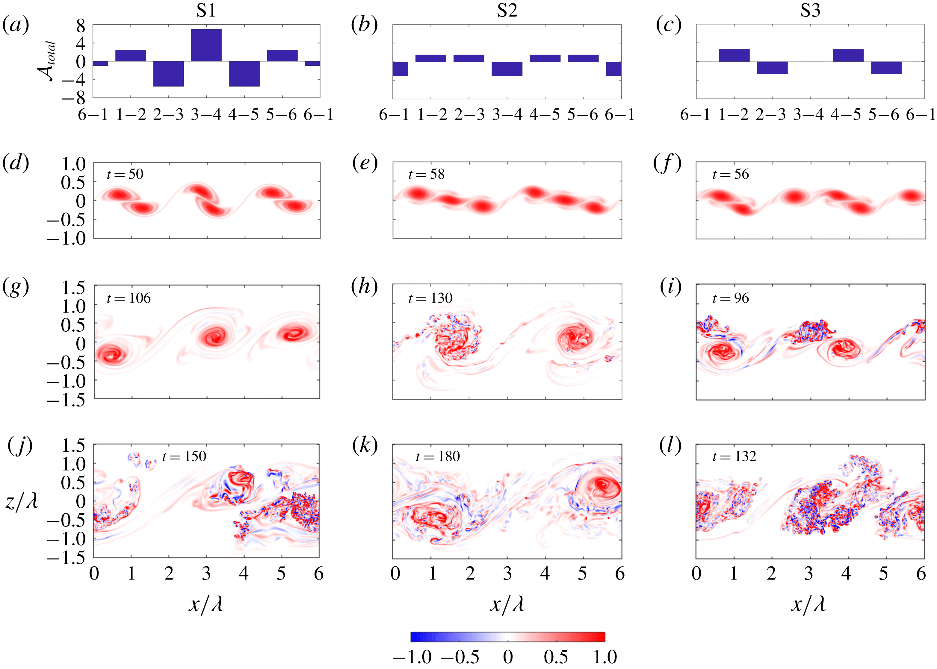
The value of $\max (|A_{total}|)$ is $7$ for S1, which is more than twice the values corresponding to S2 ( $\max (|A_{total}|)=3$ ) and S3 ( $\max (|A_{total}|)=2.6$ ). Figure 4(a) corresponds to S1, and shows a moderately positive ${\mathcal{A}}_{total}^{(1,2)}$ and ${\mathcal{A}}_{total}^{(5,6)}$ , a strongly positive ${\mathcal{A}}_{total}^{(3,4)}$ , a strongly negative ${\mathcal{A}}_{total}^{(2,3)}$ and ${\mathcal{A}}_{total}^{(4,5)}$ , and a weakly negative ${\mathcal{A}}_{total}^{(6,1)}$ . This implies vortices 1–2 and 5–6 will slowly pair, while the pairing of 3–4 would be far more rapid. Negative asymmetry implies that vortices will move away from each other, which we expect for both 2–3 and 4–5. While figure 4(a) has alternating positive and negative asymmetries (meaning the maximum extent of merging is pairing), figure 4(b) reveals a different picture – both 1–2 and 2–3 have positive asymmetries, while 3–4 has a negative one. This indicates the formation of triplets. Figure 4(c) indicates zero asymmetry for vortices 3–4 and 6–1, and are preceded by a negative asymmetry. This indicates that vortices $3$ and $6$ would not undergo pairing. The veracity of all these predictions, made solely based on initial amplitude ratios and phase shifts, needs to be substantiated using accurate numerical simulations. In fact, further late-time prediction from the initial asymmetry is also possible, and will be discussed in the following section.

Figure 4.

(a–c): Total asymmetry between consecutive wavelengths in an unstratified KH instability, inferred only from the linearized initial state. (d–f) Nonlinear evolution of KH instability using DNS during the first merging event. (g–i) Transition to turbulence in merged KH billows before the second merging event. (j–l) Turbulent phase of KH billows just before the last merging event. (a,d,g,j) Case S1, (b,e,h,k) Case S2, and (c,f,i,l) Case S3. The time $t$ is non-dimensionalized by $h_{0}/\unicode[STIX]{x0394}U$ .

3 Numerical simulations of shear instabilities and turbulence

Coherent structures appearing in transitional and turbulent shear flows can be accurately simulated using direct numerical simulations (DNS). To this end, we perform simulations using modest Reynolds number ( $Re=2000$ , where $Re\equiv \unicode[STIX]{x0394}Uh_{0}/\unicode[STIX]{x1D708}$ ; $\unicode[STIX]{x1D708}$ is the kinematic viscosity, $\unicode[STIX]{x0394}U$ and $h_{0}$ are, respectively, the shear velocity and length scales) DNS, that are more realizable in laboratory and/or industrial settings. The shear layer is initially assumed to be represented by $\bar{u}=\tanh (z)$ ; the velocity and the vertical coordinate $z$ are, respectively, non-dimensionalized by $\unicode[STIX]{x0394}U/2$ and $h_{0}/2$ . The governing 3-D incompressible, non-dimensional Navier–Stokes equations are

(3.1a,b ) $$\begin{eqnarray}\displaystyle \unicode[STIX]{x1D735}\boldsymbol{\cdot }\boldsymbol{u}=0,\quad \text{D}\boldsymbol{u}/\text{D}t=-\unicode[STIX]{x1D735}p+Re^{-1}\unicode[STIX]{x1D6FB}^{2}\boldsymbol{u}, & & \displaystyle\end{eqnarray}$$

where $\text{D}/\text{D}t$ denotes the material derivative, $\boldsymbol{u}$ denotes the dimensionless velocity vector and $p$ denotes the dimensionless pressure. These equations are solved using a pseudo-spectral code described in detail by Winters, MacKinnon & Mills (Reference Winters, MacKinnon and Mills2004) and Smyth, Nash & Moum (Reference Smyth, Nash and Moum2005). We keep the respective $x$ , $y$ and $z$ dimensions as $(L_{x},L_{y},L_{z})=(6\unicode[STIX]{x1D706},0.8\unicode[STIX]{x1D706},3\unicode[STIX]{x1D706})$ , where $\unicode[STIX]{x1D706}$ denotes the wavelength of the most unstable KH mode. Each simulation is initially perturbed with the eigenfunctions of the primary KH and its first and second subharmonics with the right phase difference. The amplitudes of the eigenfunction perturbations are sufficiently small to ensure an initial linear growth of each mode. The eigenfunction perturbations are overlaid with random perturbations (of equal or smaller order of magnitude) to trigger 3-D instabilities. The boundary conditions are periodic in both $x$ and $y$ directions and free slip at $z=0$ and $z=L_{z}$ . The number of mesh points used are: $(N_{x},N_{y},N_{z})=(1152,160,576)$ , which resolves the Kolmogorov length scale.

The DNS results for the cases S1–S3 during the first merging event are shown, respectively, in figures 4(d)–4(f). We find that the observed merging patterns are exactly as predicted by ${\mathcal{A}}_{total}^{(m,m+1)}$ , shown in figures 4(a)–4(c) – i.e. neighbouring vortices pair in the case S1, triplets form in the case S2 and alternative pairing/no-pairing occurs in the case S3. The phase relations between the primary mode and its subharmonics also have significant implications for the nonlinear evolution of the vortices in later stages and their turbulent breakdown, as shown in figures 4(g)–4(i) and 4(j)–4(l). In case S1, the merged vortices 1–2 and 5–6 undergo a second merging event; see figure 4(g). Finally, the merged vortices 3–4 coalesce with the merged vortices 1–2–5–6 to form a single vortex; this coalescence is underway in figure 4(j). The development of small-scale structures is delayed until the last merging event, since most of the energy extracted from the background shear is spent on pairing (for example, see Rahmani et al. (Reference Rahmani, Lawrence and Seymour2014)).

For case S2, during the first merging event all three vortices form a triplet. The two merged triplets are fairly symmetric and their centres are far apart; hence, they resist pairing for a relatively long time; see figure 4(h). Finally, they undergo pairing after turbulent-like structures have grown in their cores; see figure 4(k). In case S3, the unpaired vortices 3 and 6 eventually merge with vortices 4–5 and 1–2, respectively (figure 4 i). This merging event is a ‘shredding interaction’, and leads to the most vigorous disintegration of the core vortex; see figure 4(l).

Interestingly, ${\mathcal{A}}_{total}^{(m,m+1)}$ can also provide reasonable predictions of the second merging events. In other words, the large-scale 2-D patterns observed in figures 4(g)–4(i), which occur, respectively, at $t=150,\,180$ and $132$ , are predictable from the $t=0$ state (recall that ${\mathcal{A}}_{total}^{(m,m+1)}$ is always obtained from (2.9), which is the asymmetry evaluated at $t=0$ ). Considering case S1, we already found from figure 4(a) that the first merging event leads to three vortex pairs: 1–2, 3–4 and 5–6 (figure 4 d). If each primary KH billow has a circulation ${\sim}\unicode[STIX]{x1D6E4}$ , then after the first merging event, each of the merged vortices 1–2, 3–4 and 5–6 will have a circulation ${\sim}2\unicode[STIX]{x1D6E4}$ . However, ${\mathcal{A}}_{total}^{(2,3)}={\mathcal{A}}_{total}^{(4,5)}=-5.5$ , while ${\mathcal{A}}_{total}^{(6,1)}=-1$ , implying that the merged vortices 5–6 and 1–2 are expected to be far closer to each other than they are individually with 3–4; hence, the second merging would be between 1–2 and 5–6. The propensity towards this merging is observed in figure 4(g), and the merging is underway in figure 4(j), exactly as predicted.

Similar analyses can be done for the cases S2 and S3. For S2, the first merging event would lead to triplets 1–2–3 and 4–5–6; each with a circulation ${\sim}3\unicode[STIX]{x1D6E4}$ . Since ${\mathcal{A}}_{total}^{(6,1)}={\mathcal{A}}_{total}^{(3,4)}=-3$ , it implies that the two vortex triplets are far removed from each other, and hence resist second merging for a very long time; see figure 4(k). The case S3 is more interesting – the first merging produces vortex pairs 1–2 and 4–5, while vortices 3 and 6 are left out (figure 4 f). Since ${\mathcal{A}}_{total}^{(2,3)}={\mathcal{A}}_{total}^{(5,6)}=-2.6$ while ${\mathcal{A}}_{total}^{(3,4)}={\mathcal{A}}_{total}^{(6,1)}=0$ , it implies that vortex 3 would merge with 4–5, while vortex 6 would merge with 1–2. Again, this prediction is exactly found to be true in figures 4(i) and 4(l).

Figure 5.

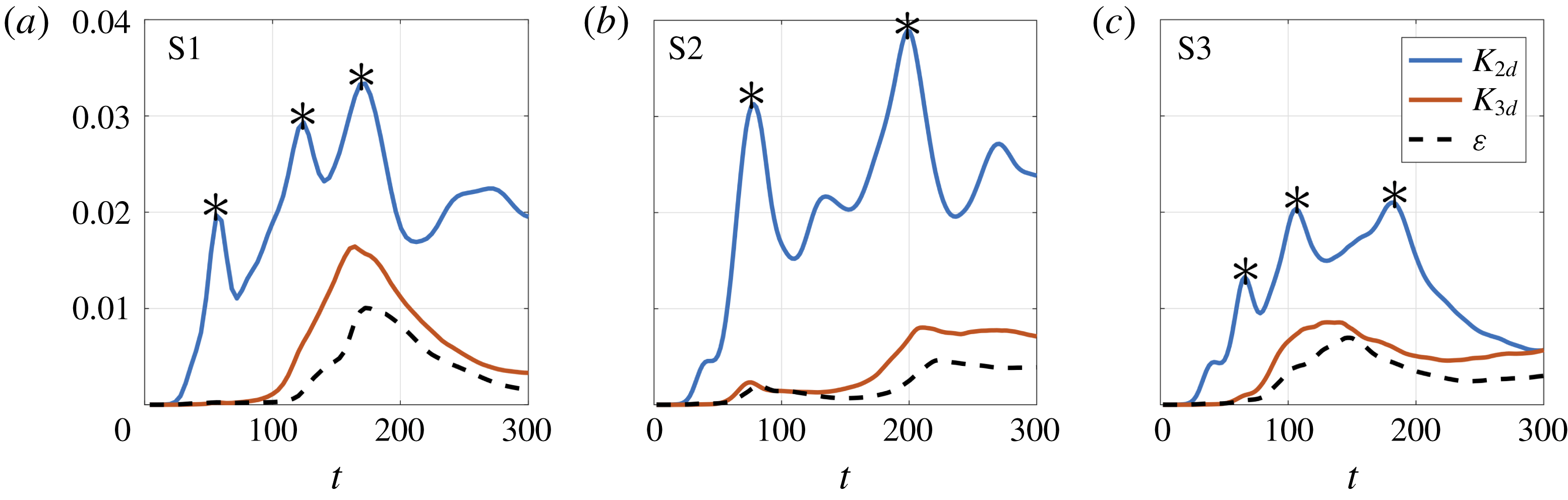
Time evolution of the dimensionless 2-D and 3-D kinetic energy, $K_{2d}$ and $K_{3d}$ , and the rate of viscous dissipation of kinetic energy, $\unicode[STIX]{x1D700}$ . The parameter $\unicode[STIX]{x1D700}$ has been multiplied by a factor of 20 for plotting. The peaks in $K_{2d}$ corresponding to merging events are marked by stars.

The growth of turbulent-like coherent structures is a consequence of 3-D motions extracting energy from the 2-D flow. To quantify the strength of the 2-D and 3-D motions, and the intensity of turbulence, we utilize the definitions of the 2-D kinetic energy: $K_{2d}=\langle \boldsymbol{u}_{2d}\boldsymbol{\cdot }\boldsymbol{u}_{2d}\rangle _{xz}$ , the 3-D kinetic energy: $K_{3d}=\langle \boldsymbol{u}_{3d}\boldsymbol{\cdot }\boldsymbol{u}_{3d}\rangle _{xyz}$ , and the rate of viscous dissipation of the total kinetic energy: $\unicode[STIX]{x1D700}=Re^{-1}\langle (\unicode[STIX]{x2202}u_{i}/\unicode[STIX]{x2202}x_{j})^{2}\rangle _{xyz}$ , with $\langle \,\rangle$ denoting the averages in the specified directions (Caulfield & Peltier Reference Caulfield and Peltier2000). In these definitions the velocity field has been partitioned into three parts: $\overline{\boldsymbol{u}}(z)=\langle \boldsymbol{u}\rangle _{xy}$ , $\boldsymbol{u}_{2d}(x,z)=\langle \boldsymbol{u}\rangle _{y}-\langle \boldsymbol{u}\rangle _{xy}$ and $\boldsymbol{u}_{3d}(x,y,z)=\boldsymbol{u}-\overline{\boldsymbol{u}}-\boldsymbol{u}_{2d}$ . The competition between $K_{2d}$ and $K_{3d}$ , and the time evolution of $\unicode[STIX]{x1D700}$ , are shown in figure 5 for the cases S1–S3. Note that after the time shown (i.e. $t>300$ ) all the motions start to decay. The intensity of the 2-D and 3-D motions and the viscous dissipation rate varies significantly between the different cases. The highest values in $K_{2d}$ correspond to the case S2, where triplets are formed and the vertical extent of the merged vortices (i.e. inertial length scale) is the largest. The major local peaks in $K_{2d}$ mark the merging events. For example, in cases S1 and S3, three merging events occur, while in the case S2, only two merging events occur. The global maxima in $K_{3d}$ and $\unicode[STIX]{x1D700}$ occur close to the last merging event in the cases S1 and S2, and close to second merging in the case S3, where the second merging involves the agglomeration of the most asymmetric vortices. The peaks in $K_{3d}$ and $\unicode[STIX]{x1D700}$ are the highest for S1, with the highest $\text{max}(|A_{total}|)$ . The values of the peaks of $K_{3d}$ are almost the same for the cases S2 and S3, which have close values of $\text{max}(|A_{total}|)$ . We therefore conclude that the initial asymmetry of the primary KH wave with respect to its subharmonic modes, given by the global measure $\text{max}(|A_{total}|)$ , has significant implications for the intensity of the ensuing turbulence. For the highest $\text{max}(|A_{total}|)$ , vortex merging occurs either earlier (as in S1 compared to S2) or more energetically (as in S1 compared to S3). In the former case, the flow has more time to develop small-scale 3-D turbulent motions before the decay starts (for example, Rahmani et al. (Reference Rahmani, Lawrence and Seymour2014)) and in the latter case, the 3-D motions can extract energy more efficiently from the 2-D flow during the active turbulent phase. In both these situations, the higher $\text{max}(|A_{total}|)$ has led to a higher intensity of turbulence.

4 Summary

In summary, we investigated the complex, multiple vortex merging patterns and ensuing turbulence characteristics in a shear layer. We have considered multiple wavelengths of the primary KH mode, and investigated the effect of higher subharmonics (and not just the first subharmonic) on the primary KH for understanding the physics of vortex merging. While related previous studies that considered vortex array (Unal & Rockwell Reference Unal and Rockwell1988; Rajagopalan & Antonia Reference Rajagopalan and Antonia2005; Baty & Keppens Reference Baty and Keppens2006; Shaabani-Ardali et al. Reference Shaabani-Ardali, Sipp and Lesshafft2019) have emphasized the role of subharmonics in vortex merging, a simple physical understanding of the underlying mechanism seems to be missing. Based on the linear theory of KH instability arising in the classic vortex-sheet profile, we have provided a mechanistic understanding of the role of subharmonics in vortex merging. We have shown that the otherwise symmetric vertical velocity field of two neighbouring wavelengths of the primary KH is rendered asymmetric by the presence of a subharmonic mode. This asymmetry, which is fully derived from the linear theory, is found to be the key in deciding the local merging patterns and their strengths. Based on the initial asymmetry of the vertical velocity profile, we have proposed an effective measure of vortex merging. Our analysis reveals that the highly nonlinear, local merging patterns in shear layers are predictable from the linearized initial state. Additionally, we show that subsequent merging patterns can also be predicted from the initial asymmetry. In fact, the highest amount of initial global asymmetry is found to yield the highest level of turbulence intensity. In summary, the main contribution of this paper is twofold – (i) to provide a simple, linear, mechanistic description of the role of subharmonics in vortex merging, and (ii) to predict nonlinear vortex merging patterns and ensuing turbulence characteristics from the linearized initial state.

In all our DNS studies reported in § 3, the primary KH and the subharmonics are overlaid with random noise of comparable amplitude, and yet our model can still accurately predict the merging patterns from linear initial conditions. Only if the random noise, that can source from other concurrent phenomena in some realistic situations, is significantly stronger (and nonlinear in nature) than the eigenfunction perturbations, do we suspect that the predictive nature of the model, which relies on the linearity of the initial state, would break down.

Our findings imply that in many realistic situations, the route to turbulence, coherent structures and turbulent characteristics are strongly dependent on the initial disturbances. Therefore, in the future, it may be possible to engineer flows to achieve optimal turbulence and mixing.