1. Introduction
Unlike annuities, in a tontine contract, longevity risk is shared among a pool of policyholders. Tontines can be attractive as they require lower safety loadings compared to annuities (e.g., Piggott et al., Reference Piggott, Valdez and Detzel2005; Sabin, Reference Sabin2010; Richter and Weber, Reference Richter and Weber2011; Newfield, Reference Newfield2014; Fullmer and Sabin, Reference Fullmer and Sabin2019). However, highly fluctuating payoffs of tontines might not be desirable for old ages (e.g., Gemmo et al., Reference Gemmo, Rogalla and Weinert2020; Weinert and Gründl, Reference Weinert and Gründl2021) and generate lower expected lifetime utilities than annuities when considering actuarially fair pricing (Milevsky and Salisbury, Reference Milevsky and Salisbury2015). Against this background, partial tontinization or combined products, such as tontines with minimum guarantees and tonuities, are proposed and have demonstrated advantages compared to annuities and tontines (e.g., Donnelly and Young, Reference Donnelly and Young2017; Chen et al., Reference Chen, Hieber and Klein2019; Chen and Rach, Reference Chen and Rach2019; Weinert and Gründl, Reference Weinert and Gründl2021).
Interestingly, despite its simple structure, the classical “tonuity” performs quite well, and policyholders do not experience significant utility losses compared to the optimal portfolio (see Chen et al. Reference Chen, Rach and Sehner2020). More concretely, the tonuity, originally proposed by Chen et al. (Reference Chen, Hieber and Klein2019), is a combination of an immediate temporary tontine and a deferred annuity, providing tontine-like payoffs till some fixed age, and annuity-like payoffs afterward. However, its current design exhibits some potential flaws and disadvantages which are to be explained in the following. First, the switching time is fixed at the moment the contract is closed. Nevertheless, the COVID-19 pandemic and medical advancements raise the question of how an unanticipated mortality/longevity shock affects policyholders’ decision on the optimal switching time ex-post. In such a changing circumstance, where the unforeseen mortality/longevity shock results in significant deviations in the predicted survival probabilities, the policyholder may suffer a loss in utility. Note that, in this paper, the terms “mortality shock” and “longevity shock” are used in a narrow sense to denote instances of mortality worsening and mortality improvement, respectively. The second possible drawback of the regular tonuity is that it requires policyholders to choose a switching time according to their risk preferences at the beginning. However, they might not possess the requisite financial knowledge to make informed decisions or may simply lack the time needed to make sound judgments. Of course, the insurance company can help policyholders make the decision. Then another question relevant to transparency pops up: How can policyholders validate whether the insurance company’s choice of switching time is optimal for them or not? In most fields of financial regulation, customer protection emphasizes the importance of transparency, including the insurance market regulation (Schwarcz, Reference Schwarcz2013). This calls for insurance products to be designed in a more transparent way.
Recognizing these limitations, this paper explores whether a more flexible design of the tonuity product can enhance its performance. We propose a modified design, termed the dynamic tonuity, which transitions from tontine-style payoffs to annuity-style payoffs upon meeting specific switching conditions based on mortality trends within a reference population (e.g., a national population). This design ensures that the switching time automatically adjusts to changes in mortality happening after the beginning of the contract. Furthermore, we can make the switching condition observable to policyholders. As an example, the switching might occur when the one-year survival probability of a reference population at some age passes a certain threshold index. The one-year survival probability is accessible in public sources, and the threshold index is specified on the contract by the insurer at the outset, ensuring transparency.
Assuming that the policyholder’s utility on the product payoffs is described by a constant relative risk aversion (CRRA) utility function, we solve the maximization problems and obtain analytic expressions for the optimal payoff structures of the dynamic tonuity. Applying a two-population mortality model, together with mortality data from UK Continuous Mortality Investigation (CMI) and Human Mortality Database (HMD), we estimate and simulate the correlated mortality rates for two populations, that is the reference population and the book population. The book population can be referred as the insurer’s annuitant pool, which is smaller than the reference population. Here, we distinguish among different cases: (i) The base case, where mortality rates develop as expected and (ii) The stress case, where after the contract is made under the base-case assumptions, some unforeseen mortality/longevity shock strikes. To illustrate the unexpected mortality shock, we use a dataset containing data from some pandemic years to estimate and project the mortality rates; while for the base case, we use a subset of the data that does not include the pandemic years’ data to obtain the mortality rates. As for the unanticipated longevity shock, it cannot be generated in a similar way as the unexpected mortality shock due to the data limitation. Instead, we create a fictional stress case with the longevity shock. Drawing insights from the mortality data and our analytical findings, we make a comprehensive discussion and comparative analysis of various tonuity products, considering them from the standpoint of the policyholder.
Our numerical results show that a well-structured dynamic tonuity can be more advantageous than a standard tonuity in a fluctuating environment. The policyholder’s degree of risk aversion plays a key role in determining contract preference, particularly in stress scenarios. Specifically, when the policyholder’s risk aversion coefficient surpasses 1 in these scenarios, those with lower risk aversion are more likely to favor the dynamic tonuity contract, as they are better able to tolerate its higher payoff volatility.
When the policyholder’s risk aversion coefficient lies within the interval (0, 1), the results concerning an unforeseen mortality shock remain unchanged. However, in the case of an unforeseen longevity shock, the effect of
 $\gamma$
on the dynamic tonuity contract’s attractiveness is not monotone. As noted by previous studies (e.g., Morin and Suárez, Reference Morin and Suárez1983; Halek and Eisenhauer, Reference Halek and Eisenhauer2001; Albert and Duffy, Reference Albert and Duffy2012), retirees generally display higher levels of risk aversion compared to younger adults. In particular, the risk aversion coefficient for individuals aged over 60 years is estimated to exceed 4 (Barsky et al., Reference Barsky, Juster, Kimball and Shapiro1997). Consequently, for the target groups of our proposed product, our findings related to relative risk aversion values greater than 1 are more relevant.
Since individuals often find it difficult to understand even basic annuity products (e.g., Brown et al., Reference Brown, Kling, Mullainathan and Wrobel2008; Lambregts and Schut, Reference Lambregts and Schut2020), the dynamic tonuity introduced in this paper may present additional complexity for policyholders. To address this challenge, we propose an approach to effectively communicate the product’s design, functionality, risks, and potential benefits. This approach leverages the key information documents (KIDs) required by European regulations for all packaged retail and insurance-based investment products (PRIIPs) (European Commission, 2014). These documents can help policyholders better understand the various risks associated with dynamic tonuity products.
The remainder of this paper is structured as follows: Section 2 demonstrates the disadvantage of a regular tonuity with numerical exercises. Section 3 gives the model setup for the dynamic tonuity. Moreover, we derive the premium and optimal payoffs of the dynamic tonuity. In Section 4, with reference to some thresholds, we provide numerical illustrations of the dynamic switching time and optimal payoffs of the dynamic tonuity. Afterward, we compare it with the regular one in different cases. Section 5 provides key information on the dynamic tonuity. In the last section, we conclude the main findings and implications of this paper. Additionally, several proofs, mortality models, and an exemplified key information document for the dynamic tonuity are available in the Supplementary Material available online.
2. Disadvantage(s) of a regular tonuity
The tonuity is originally introduced by Chen et al. (Reference Chen, Hieber and Klein2019), which works as a tontine before a fixed switching time (
 $\tau$
) and becomes an annuity after
 $\tau$
. In such a typical regular tonuity arrangement,
 $\tau$
is fixed at contract initiation and is determined based on the mortality assumptions established at the outset. Nevertheless, unexpected mortality shocks (such as the COVID-19 pandemic), or unexpected longevity shocks (e.g., a medical treatment breakthrough) can significantly impact human lives. If the tonuity contract is initiated before the onset of the shock, the predetermined switching time may no longer be ideal for the policyholders. Below, we analyze different cases to determine the utility losses experienced by individual policyholders when they enter into a standard regular tonuity contract, particularly in the presence of unforeseen mortality/longevity shocks.
2.1. Assumptions
Before presenting the cases, we first outline our model assumptions. We consider n identical policyholders, each endowed with an initial wealth amounting to
 $v \gt 0$
, who use their entire wealth to purchase some retirement plan. We assume that the insurers design regular tonuity contracts based on mortality rates of their policyholder pool, that is, the book population. We use
 $T^{(b)}$
for the random remaining lifetime of an individual in the book population, and
 $\mu_{x,h}^{(b)}$
to denote the corresponding stochastic force of mortality of an x-year old in year h. Correspondingly,
 $\mathbb{E}^{\mathbb{P}} \left[e^{-\int_0^t \mu_{x+s,h+s}^{(b)} ds}\right]$
is the best-estimate t-year survival probability of an x-year-old in calendar year h under the real-world measure
 $\mathbb{P}$
. In addition, we assume that at the moment when the insurance contract is initiated, the insurer prices the retirement plan by some chosen risk-neutral probability measure
 $\mathbb{Q}$
, which takes both unsystematic and systematic mortality risk into account. In order to be prudent, it is reasonable to assume that survival probabilities under the pricing measure
 $\mathbb{Q}$
are larger than under the real world measure
 $\mathbb{P}$
. Specifically,
 $\mathbb{E}^{\mathbb{P}}\left[e^{-\int_0^t \mu_{x+s,h+s}^{(b)} ds} \right]\lt \mathbb{E}^{\mathbb{Q}}\left[e^{-\int_0^t \mu_{x+s,h+s}^{(b,\mathbb{Q})} ds}\right]$
for all
 $t \gt 0$
, where
 $\mu_{x,h}^{(b,\mathbb{Q})}$
denotes the stochastic force of mortality of an x-year old in year h under the measure
 $\mathbb{Q}$
. Furthermore, throughout this paper, we assume the absence of financial market risks to focus exclusively on mortality risks.
To evaluate payoffs, policyholders are assumed to be risk-averse toward the uncertain lifetime. With reference to Yaari (Reference Yaari1965), the policyholder’s expected discounted lifetime utility is introduced as
 \begin{align}U(\{b(t)\}_{t\geq 0}) :\!= \mathbb{E}^{\mathbb{P}} \left[\int_{0}^{\infty} e^{-\eta t} u(b(t)) \mathbb{1}_{\{T^{(b)}\unicode{x003E}t\}} \mathrm{d}t \right], \end{align}
where
 $\eta$
denotes the subjective discount rate of the policyholder,
 $u(\cdot)$
is a utility function and b(t) represents the product payoff to a living policyholder. In this paper, we adopt the CRRA utility function, which is typically used in the life cycle literature (e.g., Gomes et al., Reference Gomes, Kotlikoff and Viceira2008; Kim et al., Reference Kim, Maurer and Mitchell2016). That is, we assume
 \begin{align} u(y)=\frac{y^{1-\gamma}}{1-\gamma},\end{align}
with a payoff stream
 $y \geq 0$
, and a constant relative risk aversion coefficient
 $\gamma \in (0,\infty)$
adhering to
 $\gamma \neq 1$
.
2.2 A brief overview of the regular tonuity framework
Construction and Payoff. Following Chen et al. (Reference Chen, Hieber and Klein2019), a regular tonuity behaves like a tontine until a fixed switching time
 $\tau$
and switches to an annuity afterward. Formally, the time-t payoff is
 \begin{align*} b_{[\tau]}(t) =\,&\mathbb{1}_{\{0\le t \unicode{x003C} \min\{\tau,T^{(b)}\}\}}\,\frac{n}{N^{(b)}(t)}\,d_{[\tau]}(t) \;+\;\mathbb{1}_{\{\tau \le t \unicode{x003C} T^{(b)}\}}\,c_{[\tau]}(t),\end{align*}
where
 $d_{[\tau]}(t)$
and
 $c_{[\tau]}(t)$
are the tontine- and annuity-specific payoffs, respectively.
Optimal Payoff Functions and Expected Utility. Under a CRRA utility function over an uncertain lifetime (cf. (2.1) and (2.2), the policyholder’s objective is to maximize the expected discounted utility of
 $\{d_{[\tau]}(t),c_{[\tau]}(t) \}_{t\ge0}$
subject to a premium constraint. In the Supplementary Material, we show that the optimal payoff streams
 $d_{[\tau]}^*(t)$
and
 $c_{[\tau]}^*(t)$
can be expressed in closed form via Lagrangian methods. The corresponding optimal expected utility is
 \[EU_{[\tau]} \;=\;\frac{\lambda_{[\tau]}}{1-\gamma}\,\cdot v,\]
where v is the premium and
 $\lambda_{[\tau]}$
is the Lagrange multiplier associated with the premium constraint.
Choosing the Switching Time. Although the optimal payoff profiles admit closed-form solutions given
 $\tau$
, one cannot solve analytically for the switching time itself (Chen et al., Reference Chen, Hieber and Klein2019; Chen et al., Reference Chen, Rach and Sehner2020). Instead, one evaluates and compares the resulting expected utilities across different
 $\tau$
-values, selecting the value
 $\tau^{*}$
that maximizes the utility.
2.3. Base and stress cases
Next, we describe different cases involving unforeseen shocks.
-
(i) The base case, where mortality assumptions do not change and there is no reassessment of the contract. The contract is optimized at the beginning. Meanwhile, the optimal switching time (
 $\tau^*$
) as well as the corresponding tontine- and annuity-specific payoffs (
$d^*_{[\tau^*]}(t)$
and
$c^*_{[\tau^*]}(t)$
) are determined and fixed.
-
(ii) The stress case, when an unforeseen mortality or longevity shock is assumed to occur in 5 years (
$t=5$
) after the contract is made (at time
$t=0$
). Below, we elaborate on the construction of the stress cases.


-
(ii-M) The stress case (M). As we know the pandemic takes away more lives than expected, especially the elderly (Yanez et al., Reference Yanez, Weiss, Romand and Treggiari2020), and mortality rates of elderly policyholders are expected to increase. In the process of generating mortality rates for the base case and the stress case, the stressed mortality rates are estimated and projected using a dataset encompassing calendar years that include some pandemic years; while the base case mortality rates are derived from a subset of data that excludes the years affected by the pandemic.
-
(ii-L) The stress case (L). In contrast to the unexpected mortality shock, we create a stress case in terms of an unexpected longevity shock. Due to data limitations, we are not able to create such a case using real mortality data. Instead, we generate a fictitious case by introducing a safety buffer to the mortality trends derived from the base-case mortality model (calibrated using the subset of data excluding pandemic years). Given that mortality improvements tend to occur gradually, driven by factors such as medical advancements, the unexpected longevity shock is constructed to be less pronounced compared to the unforeseen mortality shock.
We apply the Age-Period-Cohort model with reference to Currie (Reference Currie2006) to estimate and forecast the mortality rates for our book population under the real-world measure
 $\mathbb{P}$
. The relevant data are sourced from the CMI and HMD. To maintain focus on our primary research question, the detailed methodology is provided in the Supplementary Material available online. Figure 1 depicts the expected t-year survival probabilities of 65-year-old policyholders in the book population in (i), (ii-M), and (ii-L). Since the unforeseen shock occurs at time
 $t=5$
(i.e. when these policyholders turn 70), the expected t-year survival probabilities in the first five years are the same across different cases. As explained earlier, the expected t-year book survival probabilities in the stress case (M) are lower than those in the base case. Not surprisingly, the survival probabilities under the stress case (L) are the highest among these three cases.
Expected t-year survival probabilities of the 65-year-old in the book population under different cases. The red, green, and blue curves represent the expected t-year book survival probabilities in the base case, stress case (M), and stress case (L), respectively. The x-axis represents the year(s) after age 65.

Then, an individual’s expected utility at time
 $t=5$
is given by
 \begin{align} EU_{\{bookstr,\tau^*\}}= \begin{cases} \mathbb{E}^{\mathbb{P}}\left[\int_{5}^{\tau^*} \mathbb{1}_{\{\widehat{T}^{(b)}\unicode{x003E}t\}} e^{- \eta (t-5)} u\left(\frac{n d^*_{[\tau^*]}(t) }{\widehat{N}^{(b)}(t)}\right) \mathrm{d}t \mid\widehat{T}^{(b)}\unicode{x003E}5 \right] & \\ + \mathbb{E}^{\mathbb{P}}\left[\int_{\tau^*}^\infty \mathbb{1}_{\{\widehat{T}^{(b)}\unicode{x003E}t \}} e^{- \eta (t-5)} u\left( c^*_{[\tau^*]}(t) \right)\mathrm{d}t\mid \widehat{T}^{(b)}\unicode{x003E}5 \right],& \text{ if}\; \tau^*\geq 5 \\ \mathbb{E}^{\mathbb{P}}\left[\int_{5}^\infty \mathbb{1}_{\{\widehat{T}^{(b)}\unicode{x003E}t \}} e^{- \eta (t-5)} u\left( c^*_{[\tau^*]}(t) \right)\mathrm{d}t\mid \widehat{T}^{(b)}\unicode{x003E}5 \right], & \text{if}\; \tau^* \unicode{x003C} 5, \end{cases}\end{align}
where
 $\widehat{N}^{(b)}(t)$
is the number of pool members in case (ii-M or ii-L), and
 $\widehat{T}^{(b)}$
is the corresponding remaining lifetime. We estimate
 $\widehat{N}^{(b)}(5)$
using the best-estimate book survival probabilities of the first 5 years when no shock exists.
Expected utility of the re-optimized contract in the stress case. Given the stress cases (ii-M) and (ii-L) described above, where mortality rates increase in case of an unexpected mortality shock (or decrease with an unexpected longevity shock), at time
 $t=5$
, policyholders reassess their contract immediately. Unlike (2.3), they now alter their payoffs and the switching time according to the shock. The recomputed optimal switching time
 $\widehat{\tau}$
is given by maximizing the expected utility of the policyholder given the information of the shock. And we mark the corresponding optimal payoff streams as
 $\widehat{d}_{[\widehat{\tau}]}(t)$
and
 $\widehat{c}_{[\widehat{\tau}]}(t)$
. Then the expected utility at
 $t=5$
can be calculated by
 \begin{align}EU_{\{bookreopt,\widehat{\tau} \}}&=\mathbb{E}^{\mathbb{P}}\left[\int_5^{\widehat{\tau}} \mathbb{1}_{\{\widehat{T}^{(b)}\unicode{x003E}t \}} e^{- \eta (t-5)} u\left(\frac{n \widehat{d}_{[\widehat{\tau}]}(t) }{\widehat{N}^{(b)}(t)}\right)\mathrm{d}t \mid \widehat{T}^{(b)}\unicode{x003E}5 \right] \notag \\&\quad + \mathbb{E}^{\mathbb{P}}\left[\int_{\widehat{\tau}}^\infty \mathbb{1}_{\{\widehat{T}^{(b)}\unicode{x003E}t \}} e^{- \eta (t-5)} u\left( \widehat{c}_{[\widehat{\tau}]}(t) \right)\mathrm{d}t \mid \widehat{T}^{(b)}\unicode{x003E}5 \right].\end{align}
Numerical Example
To keep the example straightforward and simple, as mentioned above, we assume that the unexpected mortality/longevity shock takes place 5 years after the contract is made, and is instantly noticed by the policyholder.
Our model is calibrated such that a plausible set of benchmark parameters is obtained. Let us consider 1000 male policyholders of the same age who join the regular tonuity plan at the beginning of 2014 (at age 65). The pool size of 1000 is based on the findings of Qiao and Sherris (Reference Qiao and Sherris2013), where a minimum pool size of 1000 is recommended to be used in group self-annuitization schemes. Each of them invests their initial wealth of 10,000 to this plan and is assumed to have a risk aversion coefficient of
 $\gamma=8$
. Since different values of
 $\gamma$
are used in the literature (e.g., Blake et al. Reference Blake, Cairns and Dowd2003; Steinorth and Mitchell Reference Steinorth and Mitchell2015; Chen et al. Reference Chen, Hieber and Klein2019), we will carry out sensitivity analyses with respect to different
 $\gamma$
and choose a relatively high value as a benchmark for illustrative purposes. The risk-free rate
 $r_f$
used for premium calculation is chosen to be 2% according to the average annual interest rate of the United Kingdom during the last five years (from 2019 to 2023) (Bank of England 2024). The subjective discount rate
 $\eta$
is assumed to be equal to the risk-free rate. In particular, this choice results in an annual subjective discount factor in the benchmark being
 $e^{-0.02} \approx 0.98$
, which is equal to the value chosen in Cocco and Gomes (Reference Cocco and Gomes2012).Footnote 1 Furthermore, we use the Sharpe ratio approach to calibrate probabilities under
 $\mathbb{Q}$
.Footnote 2 Referring to Bauer et al. (Reference Bauer, Börger and Ruß2010), who have found that the Sharpe ratio of the UK pension annuities is between 4% and 12%, we set the Sharpe ratio as 8% and different values will be examined later in sensitivity analyses. Applying the risk-neutral pricing measure
 $\mathbb{Q}$
to the optimal regular tonuity, the resulting safety loading for the optimal tontine (when
 $\tau \rightarrow \infty$
) and for the optimal annuity (when
 $\tau=0$
) are 0.018%, and 1.31%, respectively. Here we see that, using a prudent life table, the optimal tontine requires a much lower safety loading than the optimal annuity, which implies that the optimal tontine contains less longevity risk from the insurer’s perspective. The assumed parameters are summarized in Table 1.
Benchmark parameters.

Applying the projected mortality rates and the parameters from Table 1, we find the optimal switching point that maximizes the policyholder’s expected utility,
 $\tau^*=14$
. This means that, in the base case, the policyholder should optimally switch from tontine-like payoffs to annuity-like payoffs 14 years after the initial age of 65 – at the age of 79. However, with an unforeseen mortality shock such as the COVID-19 pandemic occurring at
 $t=5$
, we find that the re-optimized switching time (
 $\widehat{\tau}$
) is 31 years after the age of 70. In other words, the policyholder optimally switches from tontine-like payoffs to annuity-like payoffs at age 101, instead of 79. In addition, the re-optimized switching time with an unforeseen longevity shock is at age 70, that is switching immediately after knowing the shock. The reason for this is that when an unforeseen mortality/longevity shock occurs, resulting in mortality worsening/improving, the tontine/annuity component of the regular tonuity will be preferable.Footnote 3
Additionally, we calculate the expected utilities using Equations (2.3) and (2.4) as outlined earlier. It is observed that in the event of an unforeseen COVID-19 pandemic occurring 5 years after the contract’s effective date (ii-M), the certainty equivalence quantityFootnote 4 of the reoptimized contract’s expected utility (2.4) to the original contract’s expected utility (2.3) is 1.272. The certainty equivalence quantity is 1.236 for the case with an unexpected longevity shock (ii-L). These represent that policyholders suffer significant utility losses if they keep to the original contract under stress cases.
3. Dynamic tonuity
As mentioned before, the regular tonuity has some drawbacks. On the one hand, the predetermined “optimal” switching time for the regular tonuity, established using initial information, may not be advantageous for the policyholder when faced with evolving circumstances. On the other hand, some policyholders may find it challenging to determine the optimal switching time. To address these problems, we propose a dynamic tonuity, which relates the insurer’s portfolio (i.e., the book population) to some “bigger” portfolio (i.e. the reference population). In this case, the switching time is not fixed at the beginning. Instead, the product switches automatically from tontine to annuity after the event that triggers the switch concerning the reference population takes place. In the following, we will define the switching criterion and payoff structure, calculate the premium, and determine the optimal payoff streams of the dynamic tonuity.
3.1. The dynamic switching time and payoff structure
As mentioned before, the proposed dynamic tonuity involves two populations. Consistent with notations of the regular tonuity, we use
 $T^{(b)}$
to mark the random remaining lifetime, and
 $\mu_{x,h}^{(b)}$
to denote the stochastic forces of mortality for the insurer’s portfolio, that is the book population. Additionally, we introduce
 $T^{(r)}$
and
 $\mu_{x,h}^{(r)}$
for the reference population to set up the automatic switching criterion. In particular,
 $\mu_{x,h}^{(b)}$
and
 $\mu_{x,h}^{(r)}$
are stochastic and correlated.
In our design of the dynamic tonuity, the switch from tontine to annuity occurs when the one-year survival probability among the reference population goes over a certain threshold index. Here, we use
 $e^{-\int_0^1 \mu_{x+t+s,h+t+s}^{(r)} ds}$
to represent the one-year realized survival curve of an
 $(x+t)$
-year-old policyholder of the cohort
 $h-x$
among the reference population. The retirement payments of the dynamic tonuity switch at the random switching time
 \begin{align}\Lambda :\!= \inf \left\{t \geq 0: e^{-\int_0^1 \mu_{x+t+s,h+t+s}^{(r)} ds} \unicode{x003E} p_{x+t,h+t}^{thr} \right \},\end{align}
where
 $\{p_{x+t,h+t}^{thr}\}_{t\geq 0}$
is a threshold vector. It can be set based on, for example, the latest officially published survival probabilities. This switching condition is fully observable to the policyholders. When the survival probability of the reference population exceeds the predetermined threshold
 $\{p_{x+t,h+t}^{thr}\}_{t\geq 0}$
for the first time, the payment structure transits from tontine-like to annuity-like payments. When varying the threshold values for
 $\{p_{x+t,h+t}^{thr}\}_{t\geq 0}$
, the switching time
 $\Lambda$
can have values of 0,
 $\infty$
, or other sensible options. Establishing an exceedingly high threshold makes it almost unattainable, thereby converting the dynamic tonuity into a tontine-like arrangement. Conversely, an excessively low threshold triggers the switch right from the beginning, transforming the dynamic tonuity into an annuity-like arrangement. It is of vital importance to make a judicious choice of the threshold to ensure the emergence of reasonable values for
 $\Lambda$
. Numerical illustrations of the dynamic switching time can be found in Subsection 4.1.
Note that the random variable
 $\Lambda$
represents the realized switching time in the future. Standing at presence, we can only make predictions to get possible realizations of
 $\Lambda$
. Subsequently, we can write down the random payoff of the dynamic tonuity given a realized switching time
 $\Lambda$
as follows:
 \begin{align}\widetilde{b}_{[\Lambda]}(t)=\mathbb{1}_{\{0\leq t \unicode{x003C} \min\{\Lambda,T^{(b)}\}\}}\frac{n}{N^{(b)}(t)}d_{[\bar{\Lambda}]}(t)+\mathbb{1}_{\{\Lambda \leq t \unicode{x003C} T^{(b)}\}}c_{[\bar{\Lambda}]}(t),\end{align}
where
 $d_{[\bar{\Lambda}]}(t)$
and
 $c_{[\bar{\Lambda}]}(t)$
, respectively, represent the deterministic tontine-like payoff and the annuity-like payoff, which are determined by maximizing the policyholder’s expected lifetime utility. In this way, these payoffs depend on expectations of functions of
 $\Lambda$
(cf. Theorem 3.1).
3.2. Premium calculation and optimal payoff streams
We obtain the premium of the dynamic tonuity as the expected present value under the risk-neutral measure
 $\mathbb{Q}$
. Different from Chen et al. (Reference Chen, Hieber and Klein2019, Reference Chen, Rach and Sehner2020) where the safety loading is a fixed proportion of the fair premium, we rely on a risk-neutral pricing approach that allows the safety loading to vary with the switching time in this paper. That is, we assume that the insurer prudently selects a risk-neutral pricing measure
 $\mathbb{Q}$
that considers both unsystematic and systematic mortality risks. Thus, a safety loading is inherently incorporated into the premium of the retirement product.
More specifically, let us define
 $\mu_{x+t,h+t}^{(\mathbb{Q})} :\!= (\mu_{x+t,h+t}^{(b,\mathbb{Q})},\mu_{x+t,h+t}^{(r,\mathbb{Q})})$
, and the realized switching time under
 $\mathbb{Q}$
is given by
 \begin{align*}\Lambda^{\mathbb{Q}} :\!= \inf \left\{t \geq 0: e^{-\int_0^1 \mu_{x+t,h+t}^{(r,\mathbb{Q})} ds} \unicode{x003E} p_{x+t,h+t}^{thr} \right\}.\end{align*}
For the risk-neutral pricing, the first-hitting time which triggers the switch in the dynamic tonuity will be determined based on this measure. Accordingly, we obtain the risk-neutral price of the dynamic tonuity as follows:
 \begin{align*}P_0^{(DT,\mathbb{Q})}&=\mathbb{E}^{\mathbb{Q}}\left[\int_{0}^{\infty} e^{-r_f t} \widetilde{b}_{[\Lambda]}(t) \mathrm{d}t\right] \\&=\mathbb{E}^{\mathbb{Q}}\left[\int_{0}^{\infty} e^{-r_f t} \left( \mathbb{1}_{\{0\leq t \unicode{x003C} \min\{\Lambda^{\mathbb{Q}},T^{(b,\mathbb{Q})}\}\}} \frac{n d_{[\bar{\Lambda}]}(t)}{N^{(b,\mathbb{Q})}(t)}+\mathbb{1}_{\{\Lambda^{\mathbb{Q}} \leq t \unicode{x003C} T^{(b,\mathbb{Q})}\}}c_{[\bar{\Lambda}]}(t) \right)\mathrm{d}t \right] \\&=\int_{0}^{\infty} e^{-r_f t} \mathbb{E}^{\mathbb{Q}}\Biggl[ \mathbb{E}^{\mathbb{Q}}\Bigl[ \mathbb{1}_{\{0\leq t \unicode{x003C} \Lambda^{\mathbb{Q}}\}} \mathbb{1}_{\{0\leq t \unicode{x003C} T^{(b,\mathbb{Q})}\}} \frac{n d_{[\bar{\Lambda}]}(t)}{N^{(b,\mathbb{Q})}(t)} \\&\qquad \qquad \qquad \qquad+ \mathbb{1}_{\{\Lambda^{\mathbb{Q}} \leq t\}} \mathbb{1}_{\{ t \unicode{x003C} T^{(b,\mathbb{Q})}\}}c_{[\bar{\Lambda}]}(t) \,\, \Big \vert \,\, \{\mu_{x+t,h+t}^{(\mathbb{Q})} \}_{t \geq 0} \Bigr] \Biggr] \mathrm{d}t \\&=\int_{0}^{\infty} e^{-r_f t} \mathbb{E}^{\mathbb{Q}}\left[ \mathbb{1}_{\{0\leq t \unicode{x003C} \Lambda^{\mathbb{Q}}\}} \underbrace{\mathbb{E}^{\mathbb{Q}}\left[ \mathbb{1}_{\{0\leq t \unicode{x003C} T^{(b,\mathbb{Q})}\}} \frac{n d_{[\bar{\Lambda}]}(t)}{N^{(b,\mathbb{Q})}(t)} \,\, \Big \vert \,\, \{\mu_{x+t,h+t}^{(\mathbb{Q})} \}_{t \geq 0}\right]}_{\mathcal A} \right] \mathrm{d}t \\&\qquad + \int_{0}^{\infty} e^{-r_f t} \mathbb E^{\mathbb{Q}}\left[ \mathbb{1}_{\{\Lambda^{\mathbb{Q}} \leq t\}} \underbrace{\mathbb{E}^{\mathbb{Q}}\left[ \mathbb{1}_{\{ t \unicode{x003C} T^{(b,\mathbb{Q})}\}}c_{[\bar{\Lambda}]}(t) \,\, \Big \vert \,\, \{\mu_{x+t,h+t}^{(\mathbb{Q})} \}_{t \geq 0} \right]}_{\mathcal B} \right] \mathrm{d}t.\end{align*}
Note that the premium can be split into a tontine and an annuity part. The first conditional expectation
 $\mathcal{A}$
is given by
 \begin{align*}&\mathbb{E}^{\mathbb{Q}}\left[ \mathbb{1}_{\{0\leq t \unicode{x003C} T^{(b,\mathbb{Q})}\}} \frac{n d_{[\bar{\Lambda}]}(t)}{N^{(b,\mathbb{Q})}(t)} \,\, \Big \vert \,\, \{\mu_{x+t,h+t}^{(\mathbb{Q})} \}_{t \geq 0} \right]\\&= e^{-\int_0^t \mu_{x+s,h+s}^{(b,{\mathbb{Q}})} ds} \cdot \mathbb{E}^{\mathbb{Q}}\left[ \frac{n d_{[\bar{\Lambda}]}(t)}{N^{(b,\mathbb{Q})}(t)} \,\, \Big \vert \,\, \{\mu_{x+t,h+t}^{(\mathbb{Q})} \}_{t \geq 0},T^{(b,\mathbb{Q})}\unicode{x003E}t \right] \\&= e^{-\int_0^t \mu_{x+s,h+s}^{(b,{\mathbb{Q}})} ds} \cdot d_{[\bar{\Lambda}]}(t) \sum_{k=0}^{n-1} \frac{n }{k+1} \binom{n-1}{k} \left( e^{-\int_0^t \mu_{x+s,h+s}^{(b,{\mathbb{Q}})} ds} \right)^{k} \left( 1- e^{-\int_0^t \mu_{x+s,h+s}^{(b,{\mathbb{Q}})} ds} \right)^{n-1-k} \\&= d_{[\bar{\Lambda}]}(t) \sum_{k=1}^{n} \binom{n}{k} \left( e^{-\int_0^t \mu_{x+s,h+s}^{(b,{\mathbb{Q}})} ds} \right)^{k} \left( 1- e^{-\int_0^t \mu_{x+s,h+s}^{(b,{\mathbb{Q}})} ds} \right)^{n-k} \\&= d_{[\bar{\Lambda}]}(t) \left(1- \left( 1- e^{-\int_0^t \mu_{x+s,h+s}^{(b,{\mathbb{Q}})} ds} \right)^{n}\right).\end{align*}
The second conditional expectation
 $\mathcal{B}$
is given by
 \begin{align*}\mathbb{E}^{\mathbb{Q}}\left[ \mathbb{1}_{\{ t \unicode{x003C} T^{(b,\mathbb{Q})}\}}c_{[\bar{\Lambda}]}(t) \,\, \Big \vert \,\, \{\mu_{x+t,h+t}^{(\mathbb{Q})} \}_{t \geq 0} \right] &= c_{[\bar{\Lambda}]}(t) \mathbb{E}^{\mathbb{Q}}\left[ \mathbb{1}_{\{ t \unicode{x003C} T^{(b,\mathbb{Q})}\}}\,\, \Big \vert \,\, \{\mu_{x+t,h+t}^{(\mathbb{Q})} \}_{t \geq 0} \right]\\&= c_{[\bar{\Lambda}]}(t) e^{-\int_0^t \mu_{x+s,h+s}^{(b,{\mathbb{Q}})} ds}.\end{align*}
Putting everything together, we obtain the following expression for the premium of the dynamic tonuity under
 $\mathbb{Q}$
:
 \begin{align} P_0^{(DT,\mathbb{Q})}&= \int_{0}^{\infty} e^{-r_f t} \mathbb{E}^{\mathbb{Q}}\left[ \mathbb{1}_{\{0\leq t \unicode{x003C} \Lambda^{\mathbb{Q}}\}} d_{[\bar{\Lambda}]}(t) \left(1- \left( 1- e^{-\int_0^t \mu_{x+s,h+s}^{(b,\mathbb{Q})} ds} \right)^{n}\right) \right] \mathrm{d}t \notag \\ &\quad + \int_{0}^{\infty} e^{-r_f t} \mathbb E^{\mathbb{Q}}\left[ \mathbb{1}_{\{\Lambda^{\mathbb{Q}} \leq t\}} c_{[\bar{\Lambda}]}(t) e^{-\int_0^t \mu_{x+s,h+s}^{(b,\mathbb{Q})} ds} \right] \mathrm{d}t .\end{align}
Depending on the precise structure of
 $\mu_{x+t,h+t}^{(b,\mathbb{Q})}$
and
 $\mu_{x+t,h+t}^{(r,\mathbb{Q})}$
, the expression may be further explored. However, due to the fact that mortality rates of the book and reference population are correlated and based on our two-population stochastic mortality model (placed in the online Supplementary Material to avoid distraction), we are unable to simplify (3.3) further at this point.
The policyholder’s objective function in the framework of the dynamic tonuity can then be translated to the following mathematical expression:
 \begin{align}&\max_{d_{[\bar{\Lambda}]}(t), c_{[\bar{\Lambda}]}(t)} \mathbb{E}^{\mathbb{P}} \left[ \int_{0}^{\infty} e^{-\eta t} \left( \mathbb{1}_{\{0\leq t \unicode{x003C} \min\{\Lambda,T^{(b)}\}\}} u\left(\frac{n d_{[\bar{\Lambda}]}(t)}{N^{(b)}(t)}\right)+\mathbb{1}_{\{\Lambda \leq t \unicode{x003C} T^{(b)}\}} u \left(c_{[\bar{\Lambda}]}(t)\right) \right) \mathrm{d}t \right] \notag \\&\qquad s.t. \quad P_0^{(DT,\mathbb{Q})}=v.\end{align}
Theorem 3.1. The solution to problem (3.4) is given by
 \begin{align} d_{[\bar{\Lambda}]}^*(t)&= \left(\lambda_{[\bar{\Lambda}]} e^{(\eta-r_f) t} \frac{ \mathbb{E}^{\mathbb{Q}}\left[ \mathbb{1}_{\{0\leq t \unicode{x003C} \Lambda^{\mathbb{Q}}\}} \left(1- \left( 1- e^{-\int_0^t \mu_{x+s,h+s}^{(b,\mathbb{Q})} ds} \right)^{n}\right) \right]}{\mathbb{E}^{\mathbb{P}}\left[ \mathbb{1}_{\{0\leq t \unicode{x003C} \Lambda\}} \mathcal K_{n,\gamma}\left( e^{-\int_0^t \mu_{x+s,h+s}^{(b)} ds} \right) \right]} \right)^{-\frac{1}{\gamma}}, \end{align}
 \begin{align} c_{[\bar{\Lambda}]}^*(t) &= \left( \lambda_{[\bar{\Lambda}]} e^{(\eta-r_f) t} \frac{ \mathbb{E}^{\mathbb{Q}}\left[ \mathbb{1}_{\{\Lambda^{\mathbb{Q}} \leq t\}} e^{-\int_0^t \mu_{x+s,h+s}^{(b,\mathbb{Q})} ds} \right]}{\mathbb{E}^{\mathbb{P}}\left[ \mathbb{1}_{\{\Lambda \leq t\}} e^{-\int_0^t \mu_{x+s,h+s}^{(b)} ds} \right]} \right)^{-\frac{1}{\gamma}}, \end{align}
where
 \begin{align*} \lambda_{[\bar{\Lambda}]} &= \Biggl[\frac{1}{v} \int_{0}^{\infty} e^{-r_f t} \left( e^{(\eta-r_f) t} \frac{ \mathbb{E}^{\mathbb{Q}}\left[ \mathbb{1}_{\{0\leq t \unicode{x003C} \Lambda^{\mathbb{Q}}\}} \left(1- \left( 1- e^{-\int_0^t \mu_{x+s,h+s}^{(b,\mathbb{Q})} ds} \right)^{n}\right) \right]}{\mathbb{E}^{\mathbb{P}}\left[ \mathbb{1}_{\{0\leq t \unicode{x003C} \Lambda\}} \mathcal K_{n,\gamma}\left( e^{-\int_0^t \mu_{x+s,h+s}^{(b)} ds} \right) \right]} \right)^{-\frac{1}{\gamma}} \\ & \quad \cdot \mathbb{E}^{\mathbb{Q}}\left[ \mathbb{1}_{\{0\leq t \unicode{x003C} \Lambda^{\mathbb{Q}}\}} \left(1- \left( 1- e^{-\int_0^t \mu_{x+s,h+s}^{(b,\mathbb{Q})} ds} \right)^{n}\right) \right] \mathrm{d}t \\ & \quad + \frac{1}{v} \int_{0}^{\infty} e^{-r_f t} \left( e^{(\eta-r_f) t} \frac{ \mathbb{E}^{\mathbb{Q}}\left[ \mathbb{1}_{\{\Lambda^{\mathbb{Q}} \leq t\}} e^{-\int_0^t \mu_{x+s,h+s}^{(b,\mathbb{Q})} ds} \right]}{\mathbb{E}^{\mathbb{P}}\left[ \mathbb{1}_{\{\Lambda \leq t\}} e^{-\int_0^t \mu_{x+s,h+s}^{(b)} ds} \right]}\right)^{-\frac{1}{\gamma}} \cdot \mathbb{E}^{\mathbb{Q}}\left[ \mathbb{1}_{\{\Lambda^{\mathbb{Q}} \leq t\}} e^{-\int_0^t \mu_{x+s,h+s}^{(b,\mathbb{Q})} ds} \right] \mathrm{d}t \Biggr]^{\gamma}, \end{align*}
where
 \begin{align*} \mathcal K_{n,\gamma}\left( e^{-\int_0^t \mu_{x+s,h+s}^{(b)} ds}\right) :\!= \sum_{k=1}^{n}\binom{n}{k} \left( \frac{k}{n} \right)^{\gamma} \left( e^{-\int_0^t \mu_{x+s,h+s}^{(b)} ds} \right)^{k} \left( 1- e^{-\int_0^t \mu_{x+s,h+s}^{(b)} ds} \right)^{n-k}. \end{align*}
And the optimal level of expected utility is then given by
 \begin{align*} \frac{\lambda_{[\bar{\Lambda}]}}{1-\gamma} \cdot v. \end{align*}
Proof: See Appendix A.
4. Numerical illustration
In this section, we present numerical examples to elucidate our proposed dynamic tonuity and compare it to the regular tonuity in the base and stress cases (as defined in Subsection 2.3). We start by introducing the thresholds for the dynamic switching condition, followed by the computation of optimal payoffs of the dynamic tonuity. Subsequently, we conduct a product comparison.
4.1. Threshold and optimal payoffs
For the dynamic tonuity, we assume that the switch from tontine to annuity is triggered when the one-year survival probability of the reference population becomes higher than the threshold index. Note that the threshold index should be chosen carefully. It should make sure that, when the insurer forecasts the future possibilities at the beginning (to create the contract), there are chances that the dynamic switching time
 $\Lambda$
could be equal to 0 and chances that the switching time approaches infinity. The switching times we mention here and in the following text are under the real-world measure
 $\mathbb{P}$
. In this paper, we take the 1949 cohort as an example (they turn 65 in 2014), and set the threshold index vector as the 0.99th power of the best-estimate one-year survival probability of the
 $(65+t)$
-year-old policyholder in the reference population (i.e.
 $p_{65+t,2014+t}^{thr}=\left(\mathbb{E}\left[e^{-\int_0^1 \mu_{65+t+s,2014+t+s}^{(r)} ds}\right]\right)^{0.99}$
).Footnote 5
The switch occurs when the simulated reference one-year survival probability at age 65 and older gets larger than the threshold index for the first time. To capture various possibilities in the future, we deploy Monte Carlo simulation methods to generate 10,000 mortality rate paths for both populations in the base case, where we denote the realized switching time by
 $\Lambda_{\{base\}}$
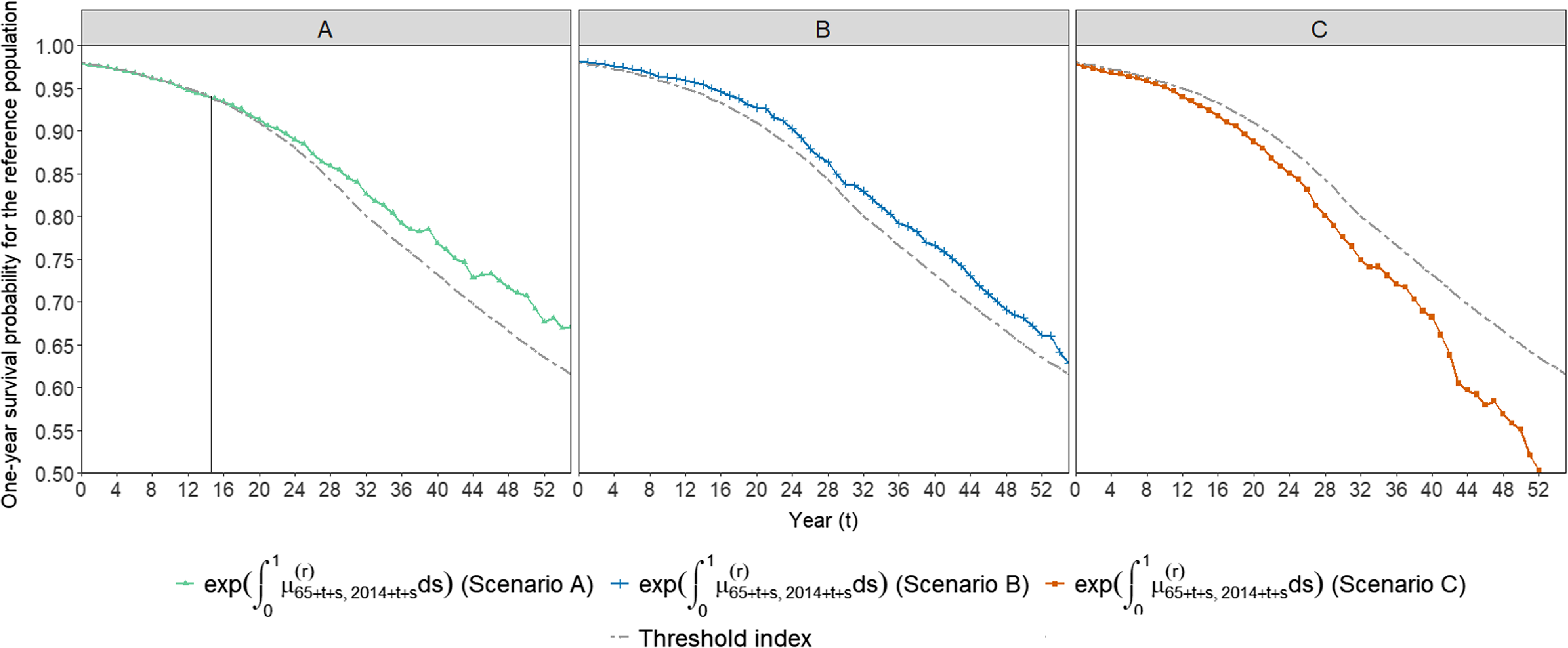
. In Figure 2, we first exhibit three situations in the base case to help us better understand the switching mechanism of the dynamic tonuity. The three situations are
-
• Situation A: The dynamic tonuity switches from tontine to annuity at age 80 (i.e.,
$\Lambda_{\{base\}}=15$
). In Panel A,
$e^{-\int_0^1 \mu_{65+t+s,2014+t+s}^{(r)} ds}$
becomes higher than the threshold index in year 15, implying
$\Lambda_{\{base\}}=15$
. -
• Situation B: The dynamic tonuity switches immediately after purchase (i.e.,
$\Lambda_{\{base\}}=0$
). Panel B displays the situation that
$e^{-\int_0^1 \mu_{65+t+s,2014+t+s}^{(r)} ds}$
is greater than the threshold index at the beginning (at age 65), such that
$\Lambda_{\{base\}}=0$
. -
• Situation C: The dynamic tonuity suggests no switching (i.e.,
$\Lambda_{\{base\}}=\infty$
). Panel C represents that
$e^{-\int_0^1 \mu_{65+t+s,2014+t+s}^{(r)} ds}$
will never hit the threshold index, thus the dynamic tonuity becomes a tontine.


Selected paths of the reference one-year survival probability for Situations A, B and C. The x-axis represents the year(s) after age 65.

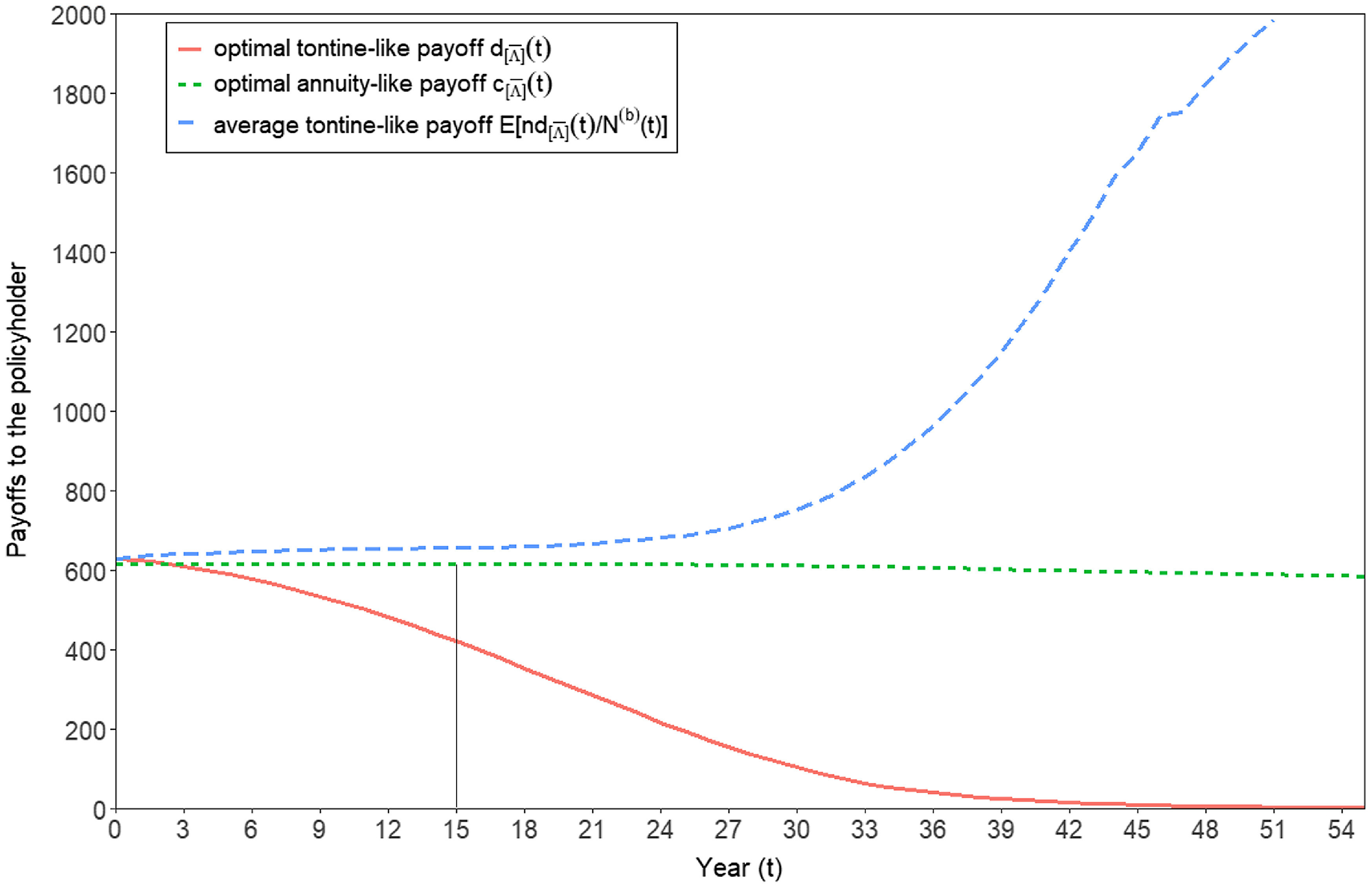
Based on the parameters stated in Table 1, we illustrate optimal payoffs for the dynamic tonuity in Figure 3. As indicated by Theorem 3.1, the optimal payoffs of the dynamic tonuity are deterministic, which depend on expectations of functions of the dynamic switching time. More specifically, for Situation A, the tontine-like payoffs (the red solid curve) are delivered to the policyholder until the 14th year, and starting from year 15, the annuity-like payoffs are provided (the green dotted curve on the right-hand side of the vertical line in Figure 3); for Situation B, since it suggests an immediate switching, the dynamic tonuity becomes an annuity and the payoffs are described completely by the green dotted curve; and for Situation C, the dynamic tonuity remains as a tontine, such that the payoffs are represented by the red solid curve.
Optimal payoffs of the dynamic tonuity in the base case. The x-axis represents the year(s) after age 65.

4.2. Product comparison
Base case
To compare the optimal dynamic tonuity with the optimal regular tonuity, we compute the certainty equivalence quantity, which signifies the quantity of optimal dynamic tonuities required to achieve an equivalent expected utility as that produced by a single optimal regular tonuity. The certainty equivalence quantity in the base case is defined by:
 \begin{align} EU_{\{bookbase, \tau^*\}}&= \int_{0}^{\infty} e^{-\eta t} \cdot \mathbb{E}^{\mathbb{P}}\left[\mathbb{1}_{\{0\leq t \unicode{x003C} \min\{\Lambda_{\{base\}},T^{(b)}\}\}} u\left(CEQ_{\{dty,base\}}\cdot \frac{n d_{[\bar{\Lambda}_{\{base\}}]}^*(t)}{N^{(b)}(t)}\right)\right] \mathrm{d}t \notag \\ &\quad + \int_{0}^{\infty} e^{-\eta t} \cdot \mathbb{E}^{\mathbb{P}}\left[ \mathbb{1}_{\{\Lambda_{\{base\}} \leq t \unicode{x003C} T^{(b)}\}} u\left(CEQ_{\{dty,base\}} \cdot c_{[\bar{\Lambda}_{\{base\}}]}^*(t) \right)\right] \mathrm{d}t \notag \\ &\quad =CEQ_{\{dty,base\}}^{1-\gamma}\cdot EU_{\{dty,base\}}, \notag \\ CEQ_{\{dyt,base\}} &=\left(\frac{EU_{\{bookbase,\tau^*\}}}{EU_{\{dyt,base\}}}\right)^{\frac{1}{1-\gamma}}. \end{align}
Here,
 $EU_{\{dyt,base\}}$
and
 $EU_{\{bookbase,\tau^*\}}$
represent the expected utilities of the optimal dynamic tonuity and the optimal regular tonuity in the base case at time
 $t=0$
, respectively.
Under the base-case assumptions, we obtain
 $CEQ_{\{dyt,base\}}=0.99901$
, which reflects that the expected utilities of the optimal dynamic tonuity and optimal regular tonuity are rather close to each other, and the former can be slightly more favorable than the latter. It is found that the optimal dynamic tonuity has a lower safety loading (0.606%) than the optimal regular tonuity (1.201%); while the payoffs provided by the optimal dynamic tonuity are more volatile over years compared to those of the optimal regular tonuity. We calculate the annual expected payoffs for these two optimal retirement products, and the volatility of the expected payoffsFootnote 6 is computed to be 30.487 for the optimal dynamic tonuity and 12.269 for the optimal regular tonuity.
Stress cases
Furthermore, we want to explore how the dynamic tonuity contract performs in a changing environment, where the survival probability decreases/increases substantially. To achieve this, we source to the “stress case” described in Subsection 2.3. In the stress case, we consider that when an unforeseen mortality/longevity shock strikes, the switching time of the dynamic tonuity may change (marked by
 $\Lambda_{\{str(M)\}}$
and
 $\Lambda_{\{str(L)\}}$
). To demonstrate the importance of an automatically adjusting switching time, we assume that all terms specified in the contract will remain unchanged. It assumes that the structure of the payoffs is optimized for long-term stability, while the switching time of the dynamic tonuity is responsive to short-term changes. For policyholders’ information, the payoffs of both regular and dynamic tonuity will be given in the contract, and thus they are considered to be fixed at the beginning.Footnote 7 The tontine-like payoffs are delivered until the new switching time (
 $\Lambda_{\{str(M)\}}$
or
 $\Lambda_{\{str(L)\}}$
), and then the annuity-like payoffs start to be provided. State differently, information on the unpredictable shocks is reflected in the new switching time, but it is not factored into the payoffs.
Let us first have a look at the dynamic switching time in the stress cases. Since we can only forecast future outcomes in the present moment, we simulate 10,000 paths as well for the stress cases resulting in 10,000 possible values of the stressed switching time. In the stress case (M), as described by Table 2, compared to the base case, the chances of no switching (
 $\infty$
) increase. This suggests that the unpredictable COVID-19 mortality shock makes the dynamic tonuity more likely to switch at a later time point or remain as a tontine. Contrarily, in the stress case (L), the suggestion of no switching is less common. As the unexpected shocks are assumed to take place at
 $t=5$
, the likelihood of switching at
 $t=0$
is not relevant for stress cases.
Chances of the extreme cases (the switching time is equal to 0 or
 $\infty$
) in 10,000 simulations in the base and stress cases. In 10,000 base case simulations, an immediate switching (
 $\Lambda_{\{base\}}=0$
results, that is dynamic tonuity becomes an annuity) for 3400 times, and no switching is obtained for 1028 times (
 $\Lambda_{\{base\}} \rightarrow \infty$
, i.e. dynamic tonuity becomes a tontine). Among the 10,000 simulations for the stress case (M), 5352 simulations suggest no switching (
 $\Lambda_{\{str(M)\}} \rightarrow \infty$
). As for the stress case (L), 902 simulations show no switching (
 $\Lambda_{\{str(L)\}} \rightarrow \infty$
). All the reported switching times are under the real-world measure
 $\mathbb{P}$
. Since the unexpected shocks occur at
 $t=5$
, the chances of switching at
 $t=0$
for stress cases are not applicable.

To make product comparisons in the stress cases, we refer to the terminologies the “dynamic tonuity contract” and “regular tonuity contract,” since the contracts are not optimal anymore now. Then the expected utility of the dynamic tonuity contract at time
 $t=5$
in the stress cases can be specified as
 \begin{align*}EU_{\{dty,str\}}&= \int_{5}^{\infty} e^{-\eta (t-5)} \mathbb{E}^{\mathbb{P}} \left[\mathbb{1}_{\{0\leq t \unicode{x003C} \min\{\Lambda_{\{str\}},\widehat{T}^{(b)}\}\}} u\left(\frac{n d_{[\bar{\Lambda}_{\{base\}}]}^*(t)}{\widehat{N}^{(b)}(t)}\right) \mid \widehat{T}^{(b)}\unicode{x003E}5 \right]\mathrm{d}t \\&\quad + \int_{5}^{\infty} e^{-\eta (t-5)} \mathbb{E}^{\mathbb{P}} \left[ \mathbb{1}_{\{\Lambda_{\{str\}} \leq t \unicode{x003C} \widehat{T}^{(b)}\}} u\left(c_{[\bar{\Lambda}_{\{base\}}]}^*(t) \right) \mid \widehat{T}^{(b)}\unicode{x003E}5 \right]\mathrm{d}t .\end{align*}
Again, we compute the corresponding certainty equivalence quantity, that is,
 \begin{align} EU_{\{bookstr, \tau^*\}}&= \left(CEQ_{\{dty,str\}}\right)^{1-\gamma} EU_{\{dty,str\}}, \end{align}
where
 $EU_{\{bookstr,\tau^*\}}$
is the expected utility of the regular tonuity contract in the stress case, which is specified in Subsection 2.3. When
 $CEQ_{\{dty,str\}}\unicode{x003C}1$
, it suggests that the dynamic tonuity contract is more favorable than the regular tonuity contract in the stress case. Further, we use
 $CEQ_{\{dty,str(M)\}}$
and
 $CEQ_{\{dty,str(L)\}}$
to denote the certainty equivalence quantity in the stress cases with an unexpected mortality shock and an unforeseen longevity shock, respectively.
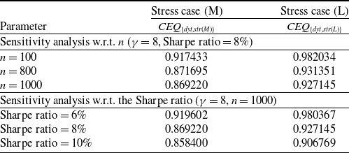
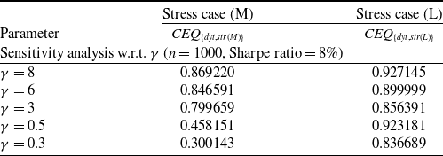
Using the parameters given in Table 1, we find that in terms of an unexpected mortality shock, the value of
 $CEQ_{\{dty,str(M)\}}$
approximates 0.869, and
 $CEQ_{\{dty,str(L)\}}$
is around 0.927 in case of an unforeseen longevity shock. This indicates that the dynamic tonuity contract can be more attractive than the regular tonuity contract in the stress cases. The reason for this is the dynamic switch of the dynamic tonuity contract, which adjusts automatically to alterations in the reference survival probabilities in stress cases.
4.3. Sensitivity analysis
In this subsection, we carry out sensitivity analyses with respect to the risk aversion coefficient
 $\gamma$
, the pool size n, and the Sharpe ratio that we have used to calibrate the probabilities under the risk-neutral measure
 $\mathbb{Q}$
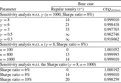
. Our results in Table 3 show that a smaller pool size n and a larger risk aversion coefficient
 $\gamma$
lead to an earlier optimal switching time of the regular tonuity, which agrees with the findings of Chen et al. (Reference Chen, Hieber and Klein2019, Reference Chen, Rach and Sehner2020). As for the product comparison, we notice that the optimal dynamic tonuity can sometimes be slightly less favorable than the optimal regular tonuity in the base case. But overall, the policyholder’s preferences for the optimal dynamic tonuity and optimal regular tonuity are rather similar. For policyholders with different risk aversion coefficients
 $\gamma$
, the optimal dynamic tonuity is more attractive to the less risk-averse ones than the optimal regular tonuity (reflected by a smaller
 $CEQ_{\{dyt,base\}}$
). It is possibly because the less risk-averse policyholders can be more tolerant of volatile payoffs than those who are more risk-averse. With respect to the pool size n, an increased pool size tends to generate slightly higher expected payoffs associated with the optimal dynamic tonuity over the years, and thus, compared to the optimal regular tonuity, the preference for the optimal dynamic tonuity intensifies. Furthermore, a higher Sharpe ratio makes the optimal dynamic tonuity more appealing than the optimal regular tonuity, potentially attributed to the increased prominence of the safety loading advantage in the dynamic version.
Sensitivity analysis of the certainty equivalence quantity with respect to different parameters (n, the Sharpe ratio and
 $\gamma$
) in the base case.

As indicated by Table 4, regarding the stress cases where an unexpected mortality or longevity shock is assumed to occur at time
 $t=5$
, with other parameters given in Table 1, variations in pool sizes and Sharpe ratios do not alter the fact that the dynamic tonuity contract remains more appealing than the regular tonuity contract (i.e.,
 $CEQ_{\{dyt,str(M)\}}\unicode{x003C}1$
and
 $CEQ_{\{dyt,str(L)\}}\unicode{x003C}1$
). A larger pool size and a higher Sharpe ratio enhance the attractiveness of the dynamic tonuity contract over the regular one in the stress cases, which are consistent with the findings in the base case.
Sensitivity analysis of the certainty equivalence quantity with respect to different parameters (n and the Sharpe ratio) in the stress cases where an unforeseen mortality or longevity shock takes place at
 $t=5$
.

We have also examined the sensitivity of results with respect to n and Sharpe ratio given
 $\gamma \in (0,1)$
. As n or Sharpe ratio increases,
 $CEQ_{\{dyt,str(M)\}}$
and
 $CEQ_{\{dyt,str(L)\}}$
increase. These results align with our observations for policyholders with risk aversion coefficients greater than 1.
According to the results presented in Table 5, when an unexpected mortality shock strikes, the dynamic tonuity contract is particularly appealing to policyholders with lower risk aversion, indicating a greater willingness to accept fluctuating payoffs. However, under an unforeseen longevity shock, the impact of
 $\gamma$
on the dynamic tonuity contract’s attractiveness is not linear. More concretely, when the policyholder’s risk aversion coefficient decreases from 3 to 0.5,
 $CEQ_{\{dyt,str(L)\}}$
gets larger instead of smaller.
Sensitivity analysis of the certainty equivalence quantity with respect to
 $\gamma$
in the stress cases where an unforeseen mortality or longevity shock takes place at
 $t=5$
.

We note that when the policyholder’s risk aversion coefficient lies in the interval of (0,1), the regular tonuity contract collapses to a tontine contract (due to an infinite switching time). This kind of policyholders may be attracted by a tontine contract initially, anticipating the entire premium allocation to be directed toward the tontine component. Contrarily, the dynamic tonuity contract takes into account the probability of various switching points. In essence, the switching time of the dynamic contract is not determined by policyholders’ preferences but is externally contingent on the trigger condition. This may affect how premiums are distributed between the annuity and tontine components. When an unexpected longevity shock occurs, the switching time is moved earlier, resulting in a shorter period of tontine-specific payoffs and a longer period of annuity-specific payoffs. This adjustment might slightly reduce the dynamic tonuity contract’s attractiveness. It is worth noting, however, that despite this, an unanticipated shock could also change the policyholder’s preferences. Since the switching time in a dynamic tonuity contract can adapt to changing conditions, it may remain the preferable option over a regular tonuity contract in the face of an unexpected longevity shock.
4.4. Discussion on further considerations
The attractiveness of retirement products can be affected by different factors as well as various interactions among them. Pre-existing income, subjective mortality beliefs, age, health risks, bequest motives, and others will generally impact the demand for annuities and tontines. The existing guaranteed income or endowed wealth serves as a financial safety net, which can reduce the need for additional stable income sources such as traditional annuities (e.g., Vidal-Meliá and Lejárraga-Garca, Reference Vidal-Meliá and Lejárraga-Garca2006; Horneff et al., Reference Horneff, Maurer and Mitchell2023; Moenig and Zhu, Reference Moenig and Zhu2024). Individuals who underestimate the life expectancy of the average tontine participants may find tontines to be more favorable according to the findings of Chen et al. (Reference Chen, Hieber and Rach2021) and Moenig and Zhu (Reference Moenig and Zhu2024).
In the context of the tonuity, which combines annuities and tontines, policyholders with pre-annuitization or optimistic subjective mortality beliefs regarding themselves might be more willing to tolerate or even prefer the more volatile payments associated with the tontine component. For policyholders with a regular tonuity, a later switching point can be an optimal choice. However, in the case of a dynamic tonuity, the switching mechanism is triggered by an objective condition, which may slightly reduce its appeal compared to a regular tonuity, where policyholders can choose their optimal switching time.
Further, policyholders’ age and health status can also influence their preference for the tontine or annuity component. Younger policyholders (with lower mortality risk) are more inclined to prefer annuities over tontines as annuities offer a secure payoff structure, which appeals more to younger individuals who may live longer and thus value guaranteed income (Moenig and Zhu Reference Moenig and Zhu2024). And healthier policyholders are likelier to prefer tontines over annuities as tontines provide benefits tied to survival, making them more appealing for individuals who perceive their survival probability as higher than average (Moenig and Zhu, Reference Moenig and Zhu2024). These may ultimately impact the relative attractiveness of the dynamic tonuity compared to the regular tonuity in the base case.
In terms of the bequest motives, Chen and Rach (Reference Chen and Rach2022) found that incorporating bequests directly into retirement products like annuities and tontines increases their attractiveness to both policyholders and insurers. Since tonuities blend elements of both tontines and annuities, we expect similar results when the bequest motive is considered, consistent with Chen and Rach (Reference Chen and Rach2022)’s findings.
Last but not least, this paper aims to emphasize that, in the face of unforeseen shocks, a well-designed dynamic tonuity may outperform a regular tonuity, particularly regarding its predetermined switching time. The dynamic tonuity, featuring an embedded dynamic switching mechanism, can excel in these stress scenarios. In the absence of such shocks, our numerical examples suggest that the performance of both the regular and dynamic tonuities is relatively similar, regardless of the factors discussed.
5. Key information of dynamic tonuities
Product complexity seems to be a barrier to annuity take-up (e.g., Brown et al., Reference Brown, Kapteyn, Luttmer, Mitchell and Samek2021) and people have a hard time understanding plain vanilla annuities (e.g., Brown et al., Reference Brown, Kling, Mullainathan and Wrobel2008; Lambregts and Schut, Reference Lambregts and Schut2020). This naturally raises the question of whether the dynamic tonuity described in this paper might perhaps be too complex for policyholders to understand. Therefore, we dedicate this section to describing one approach to how policyholders can be informed about the design and functioning as well as the risks and chances involved in the product. For this, we build upon the key information documents (KIDs) prescribed by European legislation for all packaged retail and insurance-based investment products (PRIIPs) (European Commission 2014). A template of these key information documents is available at European Commission (2017).
Apart from qualitative information on the product, its provider, and the intended investor, PRIIP-KIDs provide a summary risk indicator (SRI), a number ranging from 1 to 7, where 1 represents the lowest and 7 is the highest risk category. This SRI is calculated from a market risk value (MRV) and a credit risk value (CRV), where the MRV is determined from the distance of the 2.5%-value-at-risk (VaR) to the mean of the probability density function of the policyholder’s return and the CRV is determined using credit ratings from certified rating agencies. Naturally, dynamic tonuities contain both sources of risk, but additionally carry mortality risk, requiring the introduction of a mortality risk value, as already pointed out in Chen et al. (Reference Chen, Daskal and Rach2024). However, measuring all three sources of risk is beyond the scope of this article, especially since we are omitting the first two sources. Additionally, developing a universally applicable method for determining the mortality risk value would deserve a paper on its own.
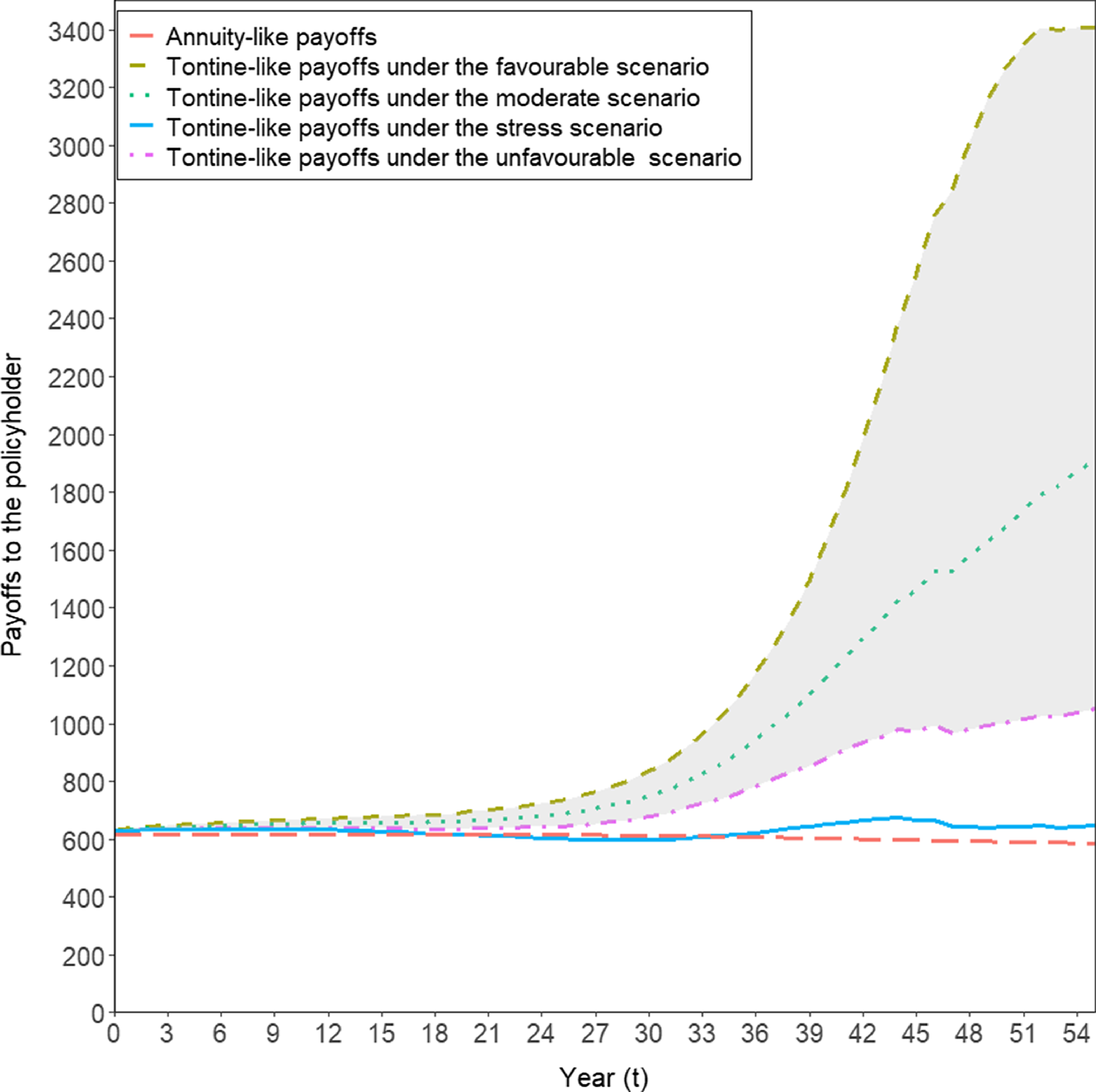
Performance scenario analysis for the policyholder’s payoffs. The red long dashed line, green short dashed line, blue dotted line, purple dotted-dashed line, and blue solid line, respectively, represent the annuity-specified and tontine-specified payoffs in the favorable, moderate, unfavorable, and stress scenarios. The grey area is the interdecile range of tontine payoffs.

In addition to the SRI, PRIIP-KIDs show four performance scenarios of the policyholder’s payoffs (European Commission 2017):
-
• “a favorable scenario” (corresponding to the 90%-VaR of the policyholder’s payoffs)
-
• “a moderate scenario” (corresponding to the 50%-VaR of the policyholder’s payoffs)
-
• “an unfavorable scenario” (corresponding to the 10%-VaR of the policyholder’s payoffs)
-
• “a stress scenario” (corresponding to the 5%-VaR of the policyholder’s payoffs under stressed assumptions)
While the above scenarios refer to the policyholder’s return at maturity, we extend the existing approach to showing confidence intervals of retirement benefits over time. For the first three scenarios, we rely on the base case. For the stress scenario, dealing with longevity risk, we rely on the longevity shock case.
Figure 4 exhibits the performance scenario analysis for the policyholder’s payoffs. The tontine-specified payoffs are shown in different scenarios. These payoffs are distributed among the policyholder pool. The distribution of payoffs to an individual surviving policyholder is provided. The blue dotted line represents the payoffs under the moderate scenario, and the gray area represents the interdecile range of these payoffs. At any given time
 $t\in[0,55]$
, the green short dashed line and purple dotted-dashed line indicate the 90% and 10% quantiles, respectively, of the payoffs to the policyholder, that is the tontine-specified payoffs under the favorable and unfavorable scenarios, respectively, as mentioned above. By age 95 (i.e.
 $t = 30$
), this range is around [680.09, 835.28], which might disappoint the risk-averse policyholders at this stage as they would prefer more stable payoffs, that is, the annuity-specified payoffs (see the red long dashed line).
For further information, we have additionally provided an exemplified Key Information Document in the Supplementary Material.
6. Conclusion
While the tonuity introduced by Chen et al. (Reference Chen, Hieber and Klein2019) has turned out to be a sound retirement product combining the advantages of annuities and tontines (Chen et al., Reference Chen, Rach and Sehner2020), it does exhibit some drawbacks in the light of an unexpected mortality shock (e.g., the recent COVID-19 pandemic) or an unanticipated longevity shock (e.g., medical advancements). Most importantly, the switching time has to be chosen at contract initiation, requiring policyholders to make a decision for the entire retirement phase based on information on mortality available at time 0. We suggest a modified version of the tonuity that contains an automatic switching time depending on the mortality experienced in a reference population, which we call dynamic tonuity. We derive the utility-maximizing payoff structures of this product for a general (random) switching time and demonstrate numerically how a properly designed dynamic tonuity can lead to higher levels of expected utility than a regular tonuity in a changing environment with mortality or longevity shocks. To improve policyholders’ understanding of our proposed product, we rely on the PRIIP-KIDs required by European legislation and show the key performance scenarios for dynamic tonuities.
While we disregard any kind of financial market risks in this paper, a question for future research could be whether unit-linked versions of tonuities might be attractive retirement plans. For example, we could combine the unit-linked tontine design introduced in Chen et al. (Reference Chen, Nguyen and Sehner2022) with some unit-linked annuity design, such as the one considered in Chen and Rach (Reference Chen and Rach2023), for example, to form a unit-linked tonuity. This unit-linked tonuity could then operate either with a fixed switching time (as in Chen et al. Reference Chen, Hieber and Klein2019) or with a random switching time as in the present paper.
In this paper, we focus exclusively on regular and dynamic tonuities, as our aim is to demonstrate how a dynamic switching mechanism can be incorporated into tonuities, enabling them to adapt and perform better in a changing environment, rather than to identify one optimal product solution. The broader retirement landscape includes a variety of other products. Retirement plans like variable annuities, which account for financial market risk, may even surpass the products discussed in the current paper. These are also potential areas to be explored in the future research.
Supplementary material
The supplementary material for this article can be found at https://doi.org/10.1017/asb.2025.5.
Acknowledgments
We want to thank the participants of the MAF conference, taking place in Le Havre from April 4 to April 6, 2024, for fruitful discussions and comments that helped us improve earlier versions of this manuscript.
Appendix
A Proof of Theorem 3.1
Let
 $\mu_{x+t,h+t} :\!= (\mu_{x+t,h+t}^{(b)},\mu_{x+t,h+t}^{(r)})$
. The expected utility of the dynamic tonuity can be written as
 \begin{align*} &\mathbb{E}^{\mathbb{P}}\left[\int_{0}^{\infty} e^{-\eta t} \left( \mathbb{1}_{\{0\leq t \unicode{x003C} \min\{\Lambda,T^{(b)}\}\}} u\left(\frac{n d_{[\bar{\Lambda}]}(t)}{N^{(b)}(t)} \right)+\mathbb{1}_{\{\Lambda \leq t \unicode{x003C} T^{(b)}\}} u\left( c_{[\bar{\Lambda}]}(t) \right) \right)\mathrm{d}t \right] \\ & = \int_{0}^{\infty} e^{-\eta t} \mathbb{E}^{\mathbb{P}}\left[ \mathbb{1}_{\{0\leq t \unicode{x003C} \min\{\Lambda,T^{(b)}\}\}} u\left(\frac{n d_{[\bar{\Lambda}]}(t)}{N^{(b)}(t)} \right)+\mathbb{1}_{\{\Lambda \leq t \unicode{x003C} T^{(b)}\}} u\left( c_{[\bar{\Lambda}]}(t) \right) \right]\mathrm{d}t \\ &=\int_{0}^{\infty} e^{-\eta t} \mathbb{E}^{\mathbb{P}}\left[ \mathbb{1}_{\{0\leq t \unicode{x003C} \Lambda\}} \mathbb{1}_{\{0\leq t \unicode{x003C} T^{(b)}\}} u\left(\frac{n d_{[\bar{\Lambda}]}(t)}{N^{(b)}(t)} \right)+ \mathbb{1}_{\{\Lambda \leq t\}} \mathbb{1}_{\{ t \unicode{x003C} T^{(b)}\}}u\left( c_{[\bar{\Lambda}]}(t) \right) \right] \mathrm{d}t \\ &=\int_{0}^{\infty} e^{-\eta t} \mathbb{E}^{\mathbb{P}}\left[ \mathbb{E}^{\mathbb{P}}\left[ \mathbb{1}_{\{0\leq t \unicode{x003C} \Lambda\}} \mathbb{1}_{\{0\leq t \unicode{x003C} T^{(b)}\}} u\left(\frac{n d_{[\bar{\Lambda}]}(t)}{N^{(b)}(t)} \right)+ \mathbb{1}_{\{\Lambda \leq t\}} \mathbb{1}_{\{ t \unicode{x003C} T^{(b)}\}}u\left( c_{[\bar{\Lambda}]}(t) \right) \,\, \Big \vert \,\, \{\mu_{x+t,h+t} \}_{t \geq 0} \right] \right] \mathrm{d}t \\ &=\int_{0}^{\infty} e^{-\eta t} \mathbb{E}^{\mathbb{P}}\left[ \mathbb{E}^{\mathbb{P}}\left[ \mathbb{1}_{\{0\leq t \unicode{x003C} \Lambda\}} \mathbb{1}_{\{0\leq t \unicode{x003C} T^{(b)}\}} u\left(\frac{n d_{[\bar{\Lambda}]}(t)}{N^{(b)}(t)} \right) \,\, \Big \vert \,\, \{\mu_{x+t,h+t} \}_{t \geq 0} \right] \right. \\ &\quad\left. + \mathbb{E}^{\mathbb{P}}\left[ \mathbb{1}_{\{\Lambda \leq t\}} \mathbb{1}_{\{ t \unicode{x003C} T^{(b)}\}}u\left( c_{[\bar{\Lambda}]}(t) \right) \,\, \Big \vert \,\, \{\mu_{x+t,h+t} \}_{t \geq 0} \right] \right] \mathrm{d}t \\ &=\int_{0}^{\infty} e^{-\eta t} \mathbb{E}^{\mathbb{P}}\left[ \mathbb{1}_{\{0\leq t \unicode{x003C} \Lambda\}} \mathbb{E}^{\mathbb{P}}\left[ \mathbb{1}_{\{0\leq t \unicode{x003C} T^{(b)}\}} u\left(\frac{n d_{[\bar{\Lambda}]}(t)}{N^{(b)}(t)} \right) \,\, \Big \vert \,\, \{\mu_{x+t,h+t} \}_{t \geq 0} \right] \right. \\ &\quad\left. + \mathbb{1}_{\{\Lambda \leq t\}} \mathbb{E}^{\mathbb{P}}\left[ \mathbb{1}_{\{ t \unicode{x003C} T^{(b)}\}}u\left( c_{[\bar{\Lambda}]}(t) \right) \,\, \Big \vert \,\, \{\mu_{x+t,h+t} \}_{t \geq 0} \right] \right] \mathrm{d}t \\ &=\int_{0}^{\infty} e^{-\eta t} \mathbb{E}^{\mathbb{P}}\left[ \mathbb{1}_{\{0\leq t \unicode{x003C} \Lambda\}} \underbrace{\mathbb{E}^{\mathbb{P}}\left[ \mathbb{1}_{\{0\leq t \unicode{x003C} T^{(b)}\}} u\left(\frac{n d_{[\bar{\Lambda}]}(t)}{N^{(b)}(t)} \right) \,\, \Big \vert \,\, \{\mu_{x+t,h+t} \}_{t \geq 0} \right]}_{\mathcal{C}} \right] \mathrm{d}t \\ &\quad + \int_{0}^{\infty} e^{-\eta t} \mathbb{E}^{\mathbb{P}}\left[ \mathbb{1}_{\{\Lambda \leq t\}} \underbrace{\mathbb{E}^{\mathbb{P}}\left[ \mathbb{1}_{\{ t \unicode{x003C} T^{(b)}\}}u\left( c_{[\bar{\Lambda}]}(t) \right) \,\, \Big \vert \,\, \{\mu_{x+t,h+t} \}_{t \geq 0} \right]}_{\mathcal{D}} \right] \mathrm{d}t. \end{align*}
Recall
 $N^{(b)}(t)-1 \sim Bin(n-1,e^{-\int_0^t \mu_{x+s,h+s}^{(b)} ds})$
, the first conditional expectation
 $\mathcal{C}$
is given by
 \begin{align*} &\mathbb{E}^{\mathbb{P}}\left[ \mathbb{1}_{\{0\leq t \unicode{x003C} T^{(b)}\}} u\left(\frac{n d_{[\bar{\Lambda}]}(t)}{N^{(b)}(t)}\right) \,\, \Big \vert \,\, \{\mu_{x+t,h+t} \}_{t \geq 0} \right]\\ &= \mathbb{E}^{\mathbb{P}}\left[ e^{-\int_0^t \mu_{x+s,h+s}^{(b)} ds} \cdot u\left(\frac{n d_{[\bar{\Lambda}]}(t)}{N^{(b)}(t)}\right) \,\, \Big \vert \,\, \{\mu_{x+t,h+t} \}_{t \geq 0}, T^{(b)} \unicode{x003E} t \right] \\ &= e^{-\int_0^t \mu_{x+s,h+s}^{(b)} ds} \cdot \mathbb{E}^{\mathbb{P}}\left[ u\left(\frac{n d_{[\bar{\Lambda}]}(t)}{N^{(b)}(t)}\right) \,\, \Big \vert \,\, \{\mu_{x+t,h+t} \}_{t \geq 0}, T^{(b)} \unicode{x003E} t \right]\\ &= e^{-\int_0^t \mu_{x+s,h+s}^{(b)} ds} \cdot u\left(d_{[\bar{\Lambda}]}(t) \right) \sum_{k=0}^{n-1} \left(\frac{n }{k+1}\right)^{1-\gamma} \binom{n-1}{k} \left( e^{-\int_0^t \mu_{x+s,h+s}^{(b)} ds} \right)^{k} \left( 1- e^{-\int_0^t \mu_{x+s,h+s}^{(b)} ds} \right)^{n-1-k}\end{align*}
 \begin{align*} &= u\left(d_{[\bar{\Lambda}]}(t) \right) \sum_{k=0}^{n-1} \left( \frac{k+1}{n} \right)^{\gamma} \binom{n}{k+1} \left( e^{-\int_0^t \mu_{x+s,h+s}^{(b)} ds} \right)^{k+1} \left( 1- e^{-\int_0^t \mu_{x+s,h+s}^{(b)} ds} \right)^{n-1-k} \\ &= u\left(d_{[\bar{\Lambda}]}(t) \right) \sum_{k=1}^{n} \left( \frac{k}{n} \right)^{\gamma} \binom{n}{k} \left( e^{-\int_0^t \mu_{x+s,h+s}^{(b)} ds} \right)^{k} \left( 1- e^{-\int_0^t \mu_{x+s,h+s}^{(b)} ds} \right)^{n-k} \\ &=: u\left(d_{[\bar{\Lambda}]}(t) \right) \mathcal K_{n,\gamma}\left( e^{-\int_0^t \mu_{x+s,h+s}^{(b)} ds} \right). \end{align*}
The second conditional expectation
 $\mathcal{D}$
is given by
 \begin{align*} \mathbb{E}^{\mathbb{P}}\left[ \mathbb{1}_{\{ t \unicode{x003C} T^{(b)}\}} u \left(c_{[\bar{\Lambda}]}(t) \right) \,\, \Big \vert \,\, \{\mu_{x+t,h+t} \}_{t \geq 0} \right] &= u \left(c_{[\bar{\Lambda}]}(t) \right) \mathbb{E}^{\mathbb{P}}\left[ \mathbb{1}_{\{ t \unicode{x003C} T^{(b)}\}}\,\, \Big \vert \,\, \{\mu_{x+t,h+t} \}_{t \geq 0} \right] \\ &= u \left(c_{[\bar{\Lambda}]}(t) \right) e^{-\int_0^t \mu_{x+s,h+s}^{(b)} ds}. \end{align*}
Putting everything together, we obtain the following expression for the expected lifetime utility of the dynamic tonuity:
 \begin{align*} &\int_{0}^{\infty} e^{-\eta t} \mathbb{E}^{\mathbb{P}}\left[ \mathbb{1}_{\{0\leq t \unicode{x003C} \Lambda\}} u\left(d_{[\bar{\Lambda}]}(t) \right) \mathcal K_{n,\gamma}\left( e^{-\int_0^t \mu_{x+s,h+s}^{(b)} ds} \right) \right] \mathrm{d}t \\ &\quad + \int_{0}^{\infty} e^{-\eta t} \mathbb{E}^{\mathbb{P}} \left[ \mathbb{1}_{\{\Lambda \leq t\}} u \left(c_{[\bar{\Lambda}]}(t) \right) e^{-\int_0^t \mu_{x+s,h+s}^{(b)} ds} \right] \mathrm{d}t \\ &= \int_{0}^{\infty} e^{-\eta t} u\left(d_{[\bar{\Lambda}]}(t) \right) \mathbb{E}^{\mathbb{P}}\left[ \mathbb{1}_{\{0\leq t \unicode{x003C} \Lambda\}} \mathcal K_{n,\gamma}\left( e^{-\int_0^t \mu_{x+s,h+s}^{(b)} ds} \right) \right] \mathrm{d}t \\ &\quad + \int_{0}^{\infty} e^{-\eta t} u \left(c_{[\bar{\Lambda}]}(t) \right) \mathbb{E}^{\mathbb{P}}\left[ \mathbb{1}_{\{\Lambda \leq t\}} e^{-\int_0^t \mu_{x+s,h+s}^{(b)} ds} \right] \mathrm{d}t. \end{align*}
A policyholder starting with an initial wealth v then faces the following optimization problem:
 \begin{align*} \max_{c_{[\bar{\Lambda}]}(t),d_{[\bar{\Lambda}]}(t)} &\int_{0}^{\infty} e^{-\eta t} u\left(d_{[\bar{\Lambda}]}(t) \right) \mathbb{E}^{\mathbb{P}}\left[ \mathbb{1}_{\{0\leq t \unicode{x003C} \Lambda\}} \mathcal K_{n,\gamma}\left( e^{-\int_0^t \mu_{x+s,h+s}^{(b)} ds} \right) \right] \mathrm{d}t \\ & + \int_{0}^{\infty} e^{-\eta t} u \left(c_{[\bar{\Lambda}]}(t) \right) \mathbb{E}^{\mathbb{P}}\left[ \mathbb{1}_{\{\Lambda \leq t\}} e^{-\int_0^t \mu_{x+s,h+s}^{(b)} ds} \right] \mathrm{d}t \end{align*}
subject to
 \begin{align*} v &= \int_{0}^{\infty} e^{-r_f t} d_{[\bar{\Lambda}]}(t) \mathbb{E}^{\mathbb{Q}}\left[ \mathbb{1}_{\{0\leq t \unicode{x003C} \Lambda\}} \left(1- \left( 1- e^{-\int_0^t \mu_{x+s,h+s}^{(b,\mathbb{Q})} ds} \right)^{n}\right) \right] \mathrm{d}t \\ &\qquad + \int_{0}^{\infty} e^{-r_f t} c_{[\bar{\Lambda}]}(t) \mathbb{E}^{\mathbb{Q}}\left[ \mathbb{1}_{\{\Lambda \leq t\}} e^{-\int_0^t \mu_{x+s,h+s}^{(b,\mathbb{Q})} ds} \right] \mathrm{d}t. \end{align*}
The first-order conditions are given by
 \begin{align*} e^{-\eta t} u'\left(d_{[\bar{\Lambda}]}(t) \right) \mathbb{E}^{\mathbb{P}}\left[ \mathbb{1}_{\{0\leq t \unicode{x003C} \Lambda\}} \mathcal K_{n,\gamma}\left( e^{-\int_0^t \mu_{x+s,h+s}^{(b)} ds} \right) \right] &= \lambda e^{-r_f t} \mathbb{E}^{\mathbb{Q}}\left[ \mathbb{1}_{\{0\leq t \unicode{x003C} \Lambda\}} \left(1- \left( 1- e^{-\int_0^t \mu_{x+s,h+s}^{(b,\mathbb{Q})} ds} \right)^{n}\right) \right] \\ e^{-\eta t} u' \left(c_{[\bar{\Lambda}]}(t) \right) \mathbb{E}^{\mathbb{P}}\left[ \mathbb{1}_{\{\Lambda \leq t\}} e^{-\int_0^t \mu_{x+s,h+s}^{(b)} ds} \right] &= \lambda e^{-r_f t} \mathbb{E}^{\mathbb{Q}}\left[ \mathbb{1}_{\{\Lambda \leq t\}} e^{-\int_0^t \mu_{x+s,h+s}^{(b,\mathbb{Q})} ds} \right]. \end{align*}
These deliver the optimal payoff functions:
 \begin{align*} d_{[\bar{\Lambda}]}^*(t) &= \left(\lambda e^{(\eta-r_f) t} \frac{ \mathbb{E}^{\mathbb{Q}}\left[ \mathbb{1}_{\{0\leq t \unicode{x003C} \Lambda\}} \left(1- \left( 1- e^{-\int_0^t \mu_{x+s,h+s}^{(b,\mathbb{Q})} ds} \right)^{n}\right) \right]}{\mathbb{E}^{\mathbb{P}}\left[ \mathbb{1}_{\{0\leq t \unicode{x003C} \Lambda\}} \mathcal K_{n,\gamma}\left( e^{-\int_0^t \mu_{x+s,h+s}^{(b)} ds} \right) \right]} \right)^{-\frac{1}{\gamma}} \\ c_{[\bar{\Lambda}]}^*(t) &= \left( \lambda e^{(\eta-r_f) t} \frac{ \mathbb{E}^{\mathbb{Q}}\left[ \mathbb{1}_{\{\Lambda \leq t\}} e^{-\int_0^t \mu_{x+s,h+s}^{(b,\mathbb{Q})} ds} \right]}{\mathbb{E}^{\mathbb{P}}\left[ \mathbb{1}_{\{\Lambda \leq t\}} e^{-\int_0^t \mu_{x+s,h+s}^{(b)} ds} \right]} \right)^{-\frac{1}{\gamma}}. \end{align*}
Plugging these expressions back into the budget constraint delivers an expression for the Lagrangian multiplier
 $\lambda$
:
 \begin{align*} \lambda^{\frac{1}{\gamma}} &= \frac{1}{v} \int_{0}^{\infty} e^{-r_f t} \left( e^{(\eta-r_f) t} \frac{ \mathbb{E}^{\mathbb{Q}}\left[ \mathbb{1}_{\{0\leq t \unicode{x003C} \Lambda\}} \left(1- \left( 1- e^{-\int_0^t \mu_{x+s,h+s}^{(b,\mathbb{Q})} ds} \right)^{n}\right) \right]}{\mathbb{E}^{\mathbb{P}}\left[ \mathbb{1}_{\{0\leq t \unicode{x003C} \Lambda\}} \mathcal K_{n,\gamma}\left( e^{-\int_0^t \mu_{x+s,h+s}^{(b)} ds} \right) \right]} \right)^{-\frac{1}{\gamma}} \\ & \quad \cdot \mathbb{E}^{\mathbb{Q}}\left[ \mathbb{1}_{\{0\leq t \unicode{x003C} \Lambda\}} \left(1- \left( 1- e^{-\int_0^t \mu_{x+s,h+s}^{(b,\mathbb{Q})} ds} \right)^{n}\right) \right] \mathrm{d}t \\ & \quad + \frac{1}{v} \int_{0}^{\infty} e^{-r_f t} \left( e^{(\eta-r_f) t} \frac{ \mathbb{E}^{\mathbb{Q}}\left[ \mathbb{1}_{\{\Lambda \leq t\}} e^{-\int_0^t \mu_{x+s,h+s}^{(b,\mathbb{Q})} ds} \right]}{\mathbb{E}^{\mathbb{P}}\left[ \mathbb{1}_{\{\Lambda \leq t\}} e^{-\int_0^t \mu_{x+s,h+s}^{(b)} ds} \right]}\right)^{-\frac{1}{\gamma}} \cdot \mathbb{E}^{\mathbb{Q}}\left[ \mathbb{1}_{\{\Lambda \leq t\}} e^{-\int_0^t \mu_{x+s,h+s}^{(b,\mathbb{Q})} ds} \right] \mathrm{d}t. \end{align*}
For the optimal level of expected utility, we obtain
 \begin{align*} &\int_{0}^{\infty} e^{-\eta t} u\left( \left(\lambda e^{(\eta-r_f) t} \frac{ \mathbb{E}^{\mathbb{Q}}\left[ \mathbb{1}_{\{0\leq t \unicode{x003C} \Lambda\}} \left(1- \left( 1- e^{-\int_0^t \mu_{x+s,h+s}^{(b,\mathbb{Q})} ds} \right)^{n}\right) \right]}{\mathbb{E}^{\mathbb{P}}\left[ \mathbb{1}_{\{0\leq t \unicode{x003C} \Lambda\}} \mathcal K_{n,\gamma}\left( e^{-\int_0^t \mu_{x+s,h+s}^{(b)} ds} \right) \right]} \right)^{-\frac{1}{\gamma}} \right) \\ &\quad\cdot \mathbb{E}^{\mathbb{P}}\left[ \mathbb{1}_{\{0\leq t \unicode{x003C} \Lambda\}} \mathcal K_{n,\gamma}\left( e^{-\int_0^t \mu_{x+s,h+s}^{(b)} ds} \right) \right] \mathrm{d}t \\ &\quad+ \int_{0}^{\infty} e^{-\eta t} u \left(\left( \lambda e^{(\eta-r_f) t} \frac{ \mathbb{E}^{\mathbb{Q}}\left[ \mathbb{1}_{\{\Lambda \leq t\}} e^{-\int_0^t \mu_{x+s,h+s}^{(b,\mathbb{Q})} ds} \right]}{\mathbb{E}^{\mathbb{P}}\left[ \mathbb{1}_{\{\Lambda \leq t\}} e^{-\int_0^t \mu_{x+s,h+s}^{(b)} ds} \right]} \right)^{-\frac{1}{\gamma}} \right) \mathbb{E}^{\mathbb{P}}\left[ \mathbb{1}_{\{\Lambda \leq t\}} e^{-\int_0^t \mu_{x+s,h+s}^{(b)} ds} \right] \mathrm{d}t \\ &= \frac{\lambda^{1-\frac{1}{\gamma}}}{1-\gamma} \Biggl[ \int_{0}^{\infty} e^{-\eta t} \left( \left( e^{(\eta-r_f) t} \frac{ \mathbb{E}^{\mathbb{Q}}\left[ \mathbb{1}_{\{0\leq t \unicode{x003C} \Lambda\}} \left(1- \left( 1- e^{-\int_0^t \mu_{x+s,h+s}^{(b,\mathbb{Q})} ds} \right)^{n}\right) \right]}{\mathbb{E}^{\mathbb{P}}\left[ \mathbb{1}_{\{0\leq t \unicode{x003C} \Lambda\}} \mathcal K_{n,\gamma}\left( e^{-\int_0^t \mu_{x+s,h+s}^{(b)} ds} \right) \right]} \right)^{-\frac{1}{\gamma}} \right)^{1-\gamma} \\ & \quad\cdot \mathbb{E}^{\mathbb{P}}\left[ \mathbb{1}_{\{0\leq t \unicode{x003C} \Lambda\}} \mathcal K_{n,\gamma}\left( e^{-\int_0^t \mu_{x+s,h+s}^{(b)} ds} \right) \right] \mathrm{d}t \\ &\quad+ \int_{0}^{\infty} e^{-\eta t} \left(\left( e^{(\eta-r_f) t} \frac{ \mathbb{E}^{\mathbb{Q}}\left[ \mathbb{1}_{\{\Lambda \leq t\}} e^{-\int_0^t \mu_{x+s,h+s}^{(b,\mathbb{Q})} ds} \right]}{\mathbb{E}^{\mathbb{P}}\left[ \mathbb{1}_{\{\Lambda \leq t\}} e^{-\int_0^t \mu_{x+s,h+s}^{(b)} ds} \right]}\right)^{-\frac{1}{\gamma}} \right)^{1-\gamma} \mathbb{E}^{\mathbb{P}}\left[ \mathbb{1}_{\{\Lambda \leq t\}} e^{-\int_0^t \mu_{x+s,h+s}^{(b)} ds} \right] \mathrm{d}t \Biggr]\\ &= \frac{\lambda^{1-\frac{1}{\gamma}}}{1-\gamma} \Biggl[ \int_{0}^{\infty} e^{-\eta t} \left( e^{(\eta-r_f) t} \frac{ \mathbb{E}^{\mathbb{Q}}\left[ \mathbb{1}_{\{0\leq t \unicode{x003C} \Lambda\}} \left(1- \left( 1- e^{-\int_0^t \mu_{x+s,h+s}^{(b,\mathbb{Q})} ds} \right)^{n}\right) \right]}{\mathbb{E}^{\mathbb{P}}\left[ \mathbb{1}_{\{0\leq t \unicode{x003C} \Lambda\}} \mathcal K_{n,\gamma}\left( e^{-\int_0^t \mu_{x+s,h+s}^{(b)} ds} \right) \right]} \right)^{1-\frac{1}{\gamma}} \\ & \quad\cdot \mathbb{E}^{\mathbb{P}}\left[ \mathbb{1}_{\{0\leq t \unicode{x003C} \Lambda\}} \mathcal K_{n,\gamma}\left( e^{-\int_0^t \mu_{x+s,h+s}^{(b)} ds} \right) \right] \mathrm{d}t \\ &\quad+ \int_{0}^{\infty} e^{-\eta t} \left( e^{(\eta-r_f) t} \frac{ \mathbb{E}^{\mathbb{Q}}\left[ \mathbb{1}_{\{\Lambda \leq t\}} e^{-\int_0^t \mu_{x+s,h+s}^{(b,\mathbb{Q})} ds} \right]}{\mathbb{E}^{\mathbb{P}}\left[ \mathbb{1}_{\{\Lambda \leq t\}} e^{-\int_0^t \mu_{x+s,h+s}^{(b)} ds} \right]}\right)^{1-\frac{1}{\gamma}} \mathbb{E}^{\mathbb{P}}\left[ \mathbb{1}_{\{\Lambda \leq t\}} e^{-\int_0^t \mu_{x+s,h+s}^{(b)} ds} \right] \mathrm{d}t \Biggr] \\ & = \frac{\lambda^{1-\frac{1}{\gamma}}}{1-\gamma} \cdot \lambda^{\frac{1}{\gamma}} \cdot v = \frac{\lambda}{1-\gamma} \cdot v. \end{align*}