





1. Introduction
In magnetic confinement fusion modelling of the wave–particle interaction underlying ion cyclotron resonance heating, it is standard to separate the time scales to come up with distinct equations describing the (fast time scale) electric field pattern associated with a given set of distribution functions of the species the plasma is composed of, and the (slow time scale) evolution of those distribution functions under the net influence of the radio frequency electric fields. These 2 aspects are intimately connected and should strictly be treated on the same footing. In practice, the assumptions made differ so the obtained solutions of the 2 equations are not fully self-consistent; most typically, it is only the integrated power density on each magnetic surface that is shared. To properly account for finite temperature and parallel as well as perpendicular gradient effects, it is customary to rely on Fourier transformation of the unknown electric field, to find appropriate expressions accounting as realistically as possible for the particle orbits and the local wave–particle interaction and finally to calculate the inverse Fourier transform to get back to physical space. That inverse transformation quickly becomes tedious, however. Hence, finding alternative means to solve the actual integro-differential wave equation is of key importance. Correctly modelling finite Larmor radius effects for modes that break the assumption that the wave phase varies only modestly over a Larmor gyration (
 $k_\perp \rho _{Larmor} \lt \lt 1$
, where
 $k_\perp$
is the perpendicular wavenumber and
 $\rho _{Larmor}$
is the Larmor radius) is a necessity since that assumption is frequently violated: the very reason for applying Ion Cyclotron Resonance Heating (ICRH) in magnetic confinement fusion machines is to create fast particle populations that do not satisfy this condition, and fusion-born populations – again at the very heart of fusion research – typically violate it as well. But rigorously describing the wave–particle interaction quickly leads to expressions containing higher-order derivatives – the treatment of which becomes cumbersome when going beyond one-dimensional application – or even forces to tackle the integro-differential wave equation ‘as is’. Inspired by the work of Jaeger (Reference Jaeger2001), some recent efforts omit that last step and simply propose to replace the continuous Fourier-space integral by a sufficiently dense discrete set of modes covering the region of
 $\boldsymbol{k}$
-space where modes are admitted. Opposite to what Jaeger did (which is to retain all possible couplings between Fourier modes, yielding a dense linear equation system matrix to be inverted), the computation effort needed can be reduced by only retaining the truly important couplings (Van Eester & Lerche Reference Van Eester and Lerche2024): as Wentzel-Kramers-Brillouin theory illustrates, interaction between wave modes requires their wave vectors locally to be close to each other. Rather than a dense matrix, the system matrix then (partly) becomes sparse. Although the absolute CPU memory and time needs increase, the relative benefit is more and more significant the more spatial dimensions are accounted for: if only
 $20\,\%$
of the couplings need to be retained in each direction, then only
 $4\,\%$
of the needs required for brute-force evaluation are needed in two dimensions and less than
 $2\,$
‰ in three dimensions; the absolute computational effort increases and quickly becomes cumbersome as the computational work essentially scales with the number of dimensions. Another classical technique relies on the use of local – rather than global – basis functions: the finite element method. For a suitable grid of points and set of local basis functions, a development in ‘quasimodes’ defined via these functions was proposed (Van Eester Reference Van Eester2026a
,
Reference Van Eesterb
) to bridge the two. This method combines the possibilities (i) to write a system in a form completely identical to that obtained when using finite elements (except for the way the coefficients of the equation are assembled), (ii) to account for the intricate
 $\boldsymbol{k}$
-space expressions already proposed decades ago to describe the impact of the confining magnetic field on the charged particles’ orbits and thereby its effect on the wave–particle interaction and (iii) allows us to cut out weak couplings to speed up the computation. Closer to the more traditional approach is what Budé proposed: when it is preferred to study the wave equation solely in physical space, he proposed to solve the integro-differential wave equation as a high-order partial differential equation by making a high-order polynomial fit of the dielectric response in
 $\boldsymbol{k}$
-space so that the inverse Fourier transform becomes trivial (see Budé Reference Budé2019; Van Eester & Lerche Reference Van Eester and Lerche2021, Reference Van Eester and Lerche2023).
Opposite to what is done in the present paper – in which well-known classical results are exploited to solve the wave equation and Fokker–Planck equation self-consistently while no new physics is presented and the burden is maximally put on the computer but analytical development is kept to a strict minimum – there is a lot of recent effort either taking a fresh look at the equations at hand and pushing the analytical treatment further or exploring alternative philosophies. Svidzinski (Reference Svidzinski2016) formulated the hot plasma dielectric response in configuration space avoiding approximations by numerically computing the plasma conductivity kernel based on the solution of the linearised Vlasov equation in a non-uniform magnetic field. By carrying out needed expressions analytically, Machielsen, Lamalle and Fukuyama proposed a method seeking to speed up this kernel approach while aiming at keeping the physics description as general as possible (Lamalle Reference Lamalle2020, Reference Lamalle2026; Machielsen Reference Machielsen2023; Fukuyama & Khan Reference Fukuyama and Khan2026). In these works an exact solution for the conductivity kernel is derived in configuration space. Machielsen’s expressions are valid to all orders in Larmor radius, and up to arbitrary cyclotron harmonic. Lamalle puts the accent on treating the parallel gradients accurately but combined with his earlier work (Lamalle Reference Lamalle1997) Larmor radius corrections can be included. Practical implementation of the most recent findings with the kernel approach is ongoing (Reman Reference Reman2026). Also seeking solutions for the coupled wave and Fokker–Planck equations is not new. Various authors have interfaced wave and Fokker–Planck equation solvers. A few examples are the coupled TORIC and SSFPQL codes by Brambilla & Bilato (Reference Bilato and Brambilla2014), the EVE-AQL suite by Dumont (Reference Dumont2009) and the combined AORSA and CQL3D codes by Jaeger & Berry (Reference Jaeger2005) and Petrov (Reference Petrov2026). An example of the exploitation of the CYRANO wave code (Lamalle Reference Lamalle1994) providing the radio frequency (RF) power depositions to solve a set of coupled Fokker–Planck equations for various beam and wave heated populations is the ICRH package in the EUROfusion European Transport Solver (see e.g. Kalupin Reference Kalupin2012; Huynh Reference Huynh2021).
Accounting for finite orbit width effects in the Fokker–Planck equation allows us to capture RF induced transport across magnetic surfaces. When doing so the Fokker–Planck takes over the role of transport equations and even generalises them: Transport equations typically describe the interaction between Maxwellian subpopulations while the (then three-dimensional) Fokker–Planck equation allows us to study transport for any population and in much more detail, making a distinction between the thermal and higher energy subpopulations. A key advantage of including the radial variation is that the description becomes more realistic: For example, omitting cross-talk between magnetic surfaces when solving sets of coupled Fokker–Planck equations has the drawback that an artificial sink term needs to be introduced when modelling neutral beam injection aside from ICRH: without a loss term, a steady state regime cannot be reached as the sum of all Coulomb collisional interactions between populations is zero (the collision operator does not create nor lose particles but just reshuffles them). In reality, accounting for the cross-talk across magnetic surfaces allows us to realistically describe the local and global particle and energy balances i.e. including the third constant of motion, energy and particles can drift in- or outwards across magnetic surfaces in the description, representing a net source or loss term. As in the actual experiment, the terms describing the net in- and outflow across the last close flux surface decide on whether reaching a steady state is even possible. But, as was shown when including ICRH in the European Transport Solver (Kalupin Reference Kalupin2012; Huynh Reference Huynh2021), accounting for the Coulomb collisional interaction between various particle populations solving coupled Fokker–Planck equations quickly becomes CPU time intensive even when somewhat simplified expressions are used. So treating the transport equations separately will likely stay the norm for at least a few years to come.
The combination of the linearised Maxwell-Vlasov equations with the quasilinear Fokker–Planck equation naturally and importantly leads us to consider non-Maxwellian velocity-space distribution functions. The idea of the present paper is to offer a fully self-consistent approach, based on common building blocks needed in the wave and Fokker–Planck equations. As a result, part of the focus is on the computation of the dielectric response for arbitrary distribution functions and its practical implementation. With the availability of increasingly powerful finite element software (examples are the finite element method (FEM) packages NGsolve (2026) and MFEM (2026)), there are also efforts exploiting such packages. Examples are the works of Vallejos (Reference Vallejos2019), Zhang (Reference Zhang2025), Maquet (Reference Maquet2026), and Zhao (Reference Zhao2026). The present paper offers a self-contained account of existing, important results pertaining to the self-consistent modelling of wave heating (wave propagation and damping + quasilinear diffusion) in the ion cyclotron resonance frequency domain in fusion plasmas. It intends to help pave the way for making use of current and next generation freewares as powerful numerical tools to combine multiscale modelling of plasmas, thereby allowing us to concentrate on the underlying physics while exploiting the present-day know-how in computer science. We underline that the paper does – up to details – not propose any new physics, nor new equations. It merely proposes a scheme allowing us to gradually upgrade the physics while guaranteeing self-consistency.
The paper is structured as follows: some basic expressions are recalled in § 2. Section 3 is devoted to discussing the case where drifts away from the magnetic surface are neglected. Section 4 generalises to the case of the axisymmetric tokamak retaining drifts. Section 5 discusses the 2 types of contributions to the basic integrals: it describes the wave–particle interaction on the slow and the fast time scales. Section 6 provides 2 examples of computations of the typical building blocks necessary to assemble the wave and Fokker–Planck equations. Section 7 is devoted to a brief summary and a minimum of discussion of the road ahead.
2. Reminder of basic expressions
In the present paper we rely on the quasilinear approach. This approach consists of making the assumption that the RF electromagnetic field oscillates rapidly at a prescribed driver frequency
 $\omega$
but represents a modest amplitude correction to the dynamics imposed by the strong, static confining magnetic field on the charged particles the plasma consists of. The distribution function
 $F$
of each of the charged particle populations can then be written as a sum of a slowly varying distribution
 $F_{\kern-1pt o}$
and a small but rapidly varying distribution function
 $f_{\textit{RF}}$
, undergoing a driven oscillation at the RF generator’s frequency. Separating the rate of change into a contribution due to the dynamics imposed by the static magnetic field
 ${\rm d}\ldots /{\rm d}t|_o$
and one at the driver frequency
 ${\rm d}\ldots /{\rm d}t|_{\textit{RF}}$
, the rate of change
 ${\rm d}F/{\rm d}t$
of
 $F$
as a function of time can then be split into 4 subparts
 \begin{align} \frac {{\rm d}F}{{\rm d}t}=\frac {{\rm d} (F_{\kern-1pt o}+f_{\textit{RF}})}{{\rm d}t}=\frac {{\rm d}F_{\kern-1pt o}}{{\rm d}t}\bigg|_o+\frac {{\rm d}\kern-2pt f_{\textit{RF}}}{{\rm d}t}\bigg|_o+\frac {{\rm d}\kern-0.5pt F_{\kern-1pt o}}{{\rm d}t}\bigg|_{\textit{RF}}+\frac {{\rm d}\kern-2pt f_{\textit{RF}}}{{\rm d}t}\bigg|_{\textit{RF}}=\ldots, \end{align}
in which the right-hand side describes the slower time scale dynamics (typically Coulomb collisions, particle injection and losses). Following the quasilinear approach and separating zero-order, linear and quadratic terms one can then isolate the linear contribution – oscillating at frequency
 $\omega$
− and find the perturbed distribution function
 \begin{align} \frac {{\rm d}\kern-1pt f_{\textit{RF}}}{{\rm d}t}\bigg|_o+\frac {{\rm d}F_{\kern-1pt o}}{{\rm d}t}\bigg|_{\textit{RF}}=0, \end{align}
or
 \begin{align} f_{\textit{RF}}=-\int {\rm d}t \frac {{\rm d}F_{\kern-1pt o}}{{\rm d}t}\bigg|_{\textit{RF}} , \end{align}
where
 \begin{align} \frac {{\rm d}\ldots }{{\rm d}t}\bigg|_{o}=\bigg[ \frac {\partial }{\partial t}+\boldsymbol{v}.\boldsymbol{\nabla} _{\boldsymbol{x}}+ \frac {q}{m}\boldsymbol{v}\times \boldsymbol{B}_o.\boldsymbol{\nabla} _{\boldsymbol{v}} \bigg] \ldots \end{align}
– in which
 ${\boldsymbol{v}}$
is the velocity,
 ${\boldsymbol{B}}_o$
the magnetic field,
 $q$
the charge and
 $m$
the mass – so the integral is along the zero-order orbit imposed by the strong, static magnetic field and the symbol
 ${\rm d}\ldots /{\rm d}t|_{\textit{RF}}$
refers to the operator
 \begin{align} \frac {{\rm d}\ldots }{{\rm d}t}\bigg|_{\textit{RF}}=\frac {q}{m}[\boldsymbol{E}+\boldsymbol{v}\times \boldsymbol{B}].\boldsymbol{\nabla} _{\boldsymbol{v}}\ldots , \end{align}
in which
 $\boldsymbol{E}$
and
 $\boldsymbol{B}$
are the RF electric and RF magnetic fields, respectively. Inserting the result in the quadratic term and integrating over all types of fast variation yields a small nonlinear net correction to the equation governing the evolution of the zero-order slowly varying distribution
 $F_{\kern-1pt o}$
. The motion of charged particles in an axisymmetric tokamak has 3 periodic aspects (Kaufman Reference Kaufman1972): the Larmor gyration, the poloidal bounce motion and the toroidal precession. The motion also has 3 constants of the motion; some detail is provided later in the text. To separate the slow variation from all oscillatory aspects of the dynamics, an integration over a full cycle is performed over the 3 corresponding angles as well as over time; we will denote the averaging by the symbol ‘
 $\lt \ldots \gt$
’. The slowly varying distribution
 $F_{\kern-1pt o}$
depends on time as well as on the quantities that are constants of the motion on the fast time scales. Moving the convective derivatives in physical and velocity space in the equation describing the distribution’s evolution to the right-hand side, yields the Fokker–Planck equation
 \begin{align} \frac {\partial F_{\kern-1pt o}}{\partial t}=Q(F_{\kern-1pt o})+C(F_{\kern-1pt o})+S-L(F_{\kern-1pt o}) , \end{align}
in which
 $Q$
,
 $C$
and
 $L$
are the RF quasilinear diffusion operator, the collision operator and the loss operator, respectively. The
 $S$
term represents the particle injection source. Filling in the expression for
 $f_{\textit{RF}}$
yields
 \begin{align} Q(F_{\kern-1pt o})=\frac {\partial F_{\kern-1pt o}}{\partial t}|_{\textit{RF}}=\frac {1}{2}Re \bigg [ \bigg\langle \boldsymbol{\nabla} _{\boldsymbol{v}}.\frac {q}{m}[\boldsymbol{E}+\boldsymbol{v}\times \boldsymbol{B}]^*\int _{-\infty }^{t}{\rm d}t' \frac {q}{m}[\boldsymbol{E}+\boldsymbol{v}\times \boldsymbol{B}].\boldsymbol{\nabla} _{\boldsymbol{v}} \bigg\rangle \bigg ] F_{\kern-1pt o}. \end{align}
All fast variation has been removed from
 $F_{\kern-1pt o}$
i.e. it only varies slowly as a function of time, either explicitly or via the 3 constants of the zero-order motion (imposed by the Lorentz force
 $q[\boldsymbol{v}\times \boldsymbol{B}_o]$
due to the static magnetic field) that vary slowly as a function of time themselves e.g. as a result of Coulomb collisions. Combining Faraday’s and Ampère’s law, the wave equation takes the form
 \begin{align} \boldsymbol{\nabla }\times \boldsymbol{\nabla }\times \boldsymbol{E} -k_o^2\boldsymbol{E}=i\omega \mu _o\bigg[\boldsymbol{J}_{\kern-2pt antenna}+q\int {\rm d}\boldsymbol{v} \boldsymbol{v} f_{\textit{RF}}\bigg] , \end{align}
where
 $k_o=\omega /c$
, with
 $c$
the speed of light,
 $\mu _o$
is the vacuum permeability and
 $\boldsymbol{J}_{\kern-2pt antenna}$
the current density on the antenna straps.
The basic philosophy exploited is to rely on variational techniques and to write the unknown electric field vector
 $\boldsymbol{E}$
in terms of a test function vector
 $\boldsymbol{F}$
locally in physical space, while equally writing the unknown distribution function
 $F_{\kern-1pt o}$
in terms of a test function
 $G$
locally in constant-of-motion space. Both equations then require us to integrate products of test functions, a procedure that can be performed once and for all. The RF magnetic field
 $\boldsymbol{B}$
can be expressed in terms of
 $\boldsymbol{E}$
and no longer explicitly appears. The equation of motion imposed by the static magnetic field can be integrated analytically (be it locally and approximately, so in a ‘patchwork’ fashion, strictly speaking) and an expression for the RF acceleration can be written based on classical results. This gives rise to the Kennel–Engelman operator acting on the electric field
 $\boldsymbol{E}$
or the test function vector
 $\boldsymbol{F}$
(Kennel & Engelman Reference Kennel and Engelman1966), labelled as
 $L_N$
in this paper for each cyclotron harmonic
 $N$
. The gradient in velocity space introduces a second operator which will be labelled here as
 $ \mathcal{\tilde {L}}_N$
and which acts on the distribution
 $F_{\kern-1pt o}$
or on the test function
 $G$
. Formally, all local contributions needed can then be written based on ‘building blocks’ involving the product
 $[\mathcal{\tilde {L}}_N(G)L_N(\boldsymbol{F})]^*L_N(\boldsymbol{E})\mathcal{\tilde {L}}_N(F_{\kern-1pt o})$
– itself a sum of products of elementary contributions only involving the finite element base functions – multiplied by a factor accounting for the local orbit integration and involving local parameters. When adopting the most commonly used approach, only the end contribution of the orbit integral is retained (`adiabatic switch-on of the
 $\boldsymbol{E}$
field’ so that events in the far past are irrelevant and the net integrated effect of events in the recent past – nearly fully – cancel out when integrating over a full RF period) in which case the dielectric response is strictly local in physical space (
 $\boldsymbol{x}$
) but still requires integrating over velocity space, while the quasilinear diffusion operator is local in velocity space (
 $\boldsymbol{v}$
) but requires an integral over the bounce orbit. Since all quantities are expressed in terms of test functions, evaluating all needed integrals merely requires summing over already computed elementary locally integrated quantities. Furthermore, including non-local effects can again be done in a ‘patchwork’ way by equally including contributions from earlier times along the particle orbit which appears in both operators, hereby replacing the assumed cancellation when integrating over a full RF period by a further upgraded approximation. To ensure orbit integrals can be evaluated accurately, choosing
 $\boldsymbol{B}_o$
-field-aligned finite element volumes is to be preferred. Treating non-local effects rigorously is far from trivial, however: because the RF time scale is several orders of magnitude different from the bounce and collisional time scales, the net effect of non-locality requires following particles accurately over a very long time, which is numerically challenging unless further analytical progress is made (see e.g. the endeavours of Lamalle (Reference Lamalle2020, Reference Lamalle2026) and Reman (Reference Reman2026)).
We will adopt the notations standardly used when describing the wave dynamics in tokamaks so
 $R$
is the major radius,
 $Z$
the height above or below the midplane,
 $\theta$
is the poloidal and
 $\varphi$
the toroidal angle. The subscripts ‘//’ and ‘
 $\perp$
’ are with respect to the static magnetic field
 $\boldsymbol{B}_o$
. When wave directionality in the plane perpendicular to the magnetic field line is studied the angle
 $\psi =\tan^{-1}[k_{\perp ,2}/k_{\perp ,1}]$
is introduced, where
 $\boldsymbol{k}$
is projected on suitably chosen orthogonal unit vectors
 $\boldsymbol{e}_{\perp ,1}$
and
 $\boldsymbol{e}_{\perp ,2}$
. Finally, the subscript ‘o’ either refers to the static component (in the case of the confining magnetic field), the slowly varying component (in the case of the distribution function) or the magnetic axis (in the case of the major radius), and
 $\varTheta$
is the angle between the parallel and the toroidal direction so
 $\cos \varTheta =B_{o,\varphi }/B_o$
and
 $\sin\!\varTheta =B_{o,\theta }/B_o$
so that
 $\boldsymbol{e}_{//}=\cos \varTheta \boldsymbol{e}_\varphi + \sin\!\varTheta \boldsymbol{e}_{\theta }$
with
 $\boldsymbol{e}_\varphi =\partial \boldsymbol{x} /\partial \varphi /|\partial \boldsymbol{x} /\partial \varphi |$
and
 $\boldsymbol{e}_\theta =\partial \boldsymbol{x} /\partial \theta /|\partial \boldsymbol{x} /\partial \theta |$
. Here,
 $\rho$
is the magnetic surface labelling parameter (half the width of the magnetic surface in the midplane is a frequent choice) so
 $\boldsymbol{\nabla }\rho / |\boldsymbol{\nabla }\rho |$
is a unit vector perpendicular to a magnetic surface. Furthermore,
 $q$
is the charge,
 $m$
the mass,
 $N$
the cyclotron harmonic and
 $n$
the toroidal mode number. We adopt the symbol
 $\mathcal{N}$
for the density.
Describing the wave–particle interaction involves physical (
 $\boldsymbol{x}$
) as well as velocity (
 $\boldsymbol{v}$
) space. The wave equation is formulated in physical space so as to obtain the wave equation coefficients; an integration over velocity is required first. The Fokker–Planck equation is formulated in terms of constants of the motion while averaging out the 3 types of rapid oscillations (gyromotion, bounce motion and toroidal precession). For an axisymmetric tokamak the 3 most commonly used constants of motion are the energy
 \begin{align} {\epsilon =mv^2/2,} \end{align}
the magnetic moment
 \begin{align} {\mu =mv_\perp ^2/[2B_o]} \end{align}
and the toroidal angular momentum (see e.g. Balescu Reference Balescu1988)
 \begin{align} p_\varphi =\varPsi -2\pi\kern-1pt m\kern-1pt R v_\varphi /q=\varPsi -2\pi\kern-1pt m\kern-1pt R_o v_{//} B_{{o,\varphi }} /[qB_o] , \end{align}
in which
 $\varPsi (\rho )$
is the poloidal magnetic flux, which is sometimes used as the flux surface labelling parameter instead of the minor radius
 $\rho$
.
The absorbed power as defined in the Fokker–Planck equation and that in the wave equation must be identical. This requires the adopted models to be sufficiently sophisticated and handled using the same approximations. The RF absorbed power for a specific species can be written as
 \begin{align} P_{abs,FP}&=\frac {\partial }{\partial t} \bigg [ \int {\rm d}\boldsymbol{v}{\rm d}\boldsymbol{x} \epsilon F_0\bigg ] \bigg |_{\textit{RF}} = \int {\rm d}\boldsymbol{v}{\rm d}\boldsymbol{x} \epsilon \frac {\partial F_{\kern-1pt o}}{\partial t}_{\textit{RF}} = \int {\rm d}\boldsymbol{v}{\rm d}\boldsymbol{x} \epsilon Q(F_{\kern-1pt o}) \nonumber \\[3pt]& = \frac {1}{2} Re\bigg [ {\int } {\rm d}\boldsymbol{v}{\rm d}\boldsymbol{x} \epsilon \boldsymbol{\nabla} _{\boldsymbol{v}} . \frac {q}{m} [\boldsymbol{E}+\boldsymbol{v}\times \boldsymbol{B}]^* \int _{-\infty }^{t}{\rm d}t' \frac {q}{m}[\boldsymbol{E}+\boldsymbol{v}\times \boldsymbol{B}] .\boldsymbol{\nabla} _{\boldsymbol{v}}F_{\kern-1pt o}\bigg ]\nonumber \\[3pt]& = - \frac {1}{2} Re\bigg [ {\int } {\rm d}\boldsymbol{v}{\rm d}\boldsymbol{x} [ \boldsymbol{\nabla} _{\boldsymbol{v}}\epsilon ] .\frac {q}{m}[ \boldsymbol{E}+\boldsymbol{v}\times \boldsymbol{B}]^* \int _{-\infty }^{t}{\rm d}t' \frac {q}{m}[ \boldsymbol{E}+\boldsymbol{v}\times \boldsymbol{B}] .\boldsymbol{\nabla} _{\boldsymbol{v}}F_{\kern-1pt o}\bigg ]\nonumber \\[3pt] & = \frac {1}{2} Re\bigg [ {\int } {\rm d}\boldsymbol{v}{\rm d}\boldsymbol{x} [ \boldsymbol{\nabla} _{\boldsymbol{v}}\epsilon ] .\frac {q}{m}[ \boldsymbol{E}+\boldsymbol{v}\times \boldsymbol{B}]^* f_{\textit{RF}}\bigg ]\nonumber \\[3pt] & = \frac {q}{2} Re\bigg [ {\int }{\rm d}\boldsymbol{v}{\rm d}\boldsymbol{x}\kern-0.8pt\boldsymbol{v} .[ \boldsymbol{E}+\boldsymbol{v}\times \boldsymbol{B}]^* f_{\textit{RF}}\bigg ]\nonumber \\[3pt] & = - \frac {q}{2} Re\bigg[{\int }{\rm d}\boldsymbol{v}{\rm d}\boldsymbol{x}\boldsymbol{v} .\boldsymbol{E}^* f_{\textit{RF}}\bigg]= - \frac {1}{2} Re\bigg[{\int }{\rm d}\boldsymbol{x}\boldsymbol{J}_{\kern-1pt plasma}^* .\boldsymbol{E} \bigg]=P_{abs,WE}{.} \end{align}
A fully self-consistent description of the wave and Fokker–Planck equations becomes possible when first evaluating common elementary ‘building blocks’ representing the interaction between an orbit and the wave. At the heart of both is the expression for how the charged particle and the wave interact. To obtain the wave equation coefficients integrations over velocity space need to be performed, locally expressing the distribution function in terms of the velocity components. To obtain the Fokker–Planck coefficients requires performing the
 $\lt \ldots \gt$
integrations. Integrations over an RF period, over a toroidal circuit and over the gyroperiod are straightforward but the integration over the bounce motion requires more attention and is a key aspect determining the level of complexity accounted for in models. Many authors have contributed to formulating the wave and Fokker–Planck equations. The present paper aims at proposing a method allowing us to solve both in a self-consistent way, the advantage being that there is no longer a need for adjustment factors to interface the wave and Fokker–Planck equations which are typically built on differing assumptions. For the time being, the building blocks the method relies on are expressed in
 $\boldsymbol{k}$
-space since that allows a direct connection to known expressions. To assemble the linear system locally corresponding to the variational form of the wave equation – and to evaluate the corresponding coefficients of the quasilinear diffusion operator – one of the following methods can e.g. be used:
-
(i) the Budé technique (Budé (Reference Budé2021); Van Eester (Reference Van Eester and Lerche2021); Maquet (Reference Maquet2026)) which makes a fit in function of the
 ${\boldsymbol{k}}$
components of the electric field
${\boldsymbol{E}}$
and the
${\boldsymbol{k}}'$
components of the test function vector
${\boldsymbol{F}}$
, and subsequently executes the inverse Fourier transform to get the dielectric response in differential form;
-
(ii) the ‘fast-AORSA’ technique (Van Eester Reference Van Eester and Lerche2024) which remains in
$\boldsymbol{k}$
-space but reduces the size of the numerical system by filtering out far coupling terms which negligibly contribute (Jaeger’s AORSA code (Jaeger Reference Jaeger2001) solves the integro-differential equation by brute force, discretising
$\boldsymbol{k}$
-space but retaining all couplings); -
(iii) the quasimodes technique (Van Eester Reference Van Eester2026b ) which exploits the fast Fourier transform of the base functions to solve the wave equation and hence allows us to exploit the finite element technique while still being able to exploit expressions for the wave–particle interaction in
$\boldsymbol{k}$
-space.


All these techniques have already been exploited in one dimension to solve the all-FLR integro-differential wave equation; here, ‘FLR’ stands for finite Larmor radius effects and ‘all’ refers to the fact that all finite Larmor radius corrections were retained when describing the interaction of fields and particles while more standard modelling truncates the expressions, typically at second-order terms in
 $k_\perp \rho _{Larmor}$
(`FLR2’;
 $k_\perp$
: perpendicular wavenumber and
 $\rho _{Larmor}$
: Larmor radius). Extension to two or three dimensions requires further speed-up to allow the technique to be efficiently exploitable in practice. This search for optimisation is presently still very much ongoing.
The corresponding Fokker–Planck terms require assembling the contributions along a particle bounce. The above building blocks are especially transparent since most Fokker–Planck models do not consider the actual differential or integro-differential operators but provide ‘homogeneous plasma’ expressions so that the quasilinear diffusion operator can simply be expressed in terms of
 $\boldsymbol{k}$
. This approach is here generalised to
 $\boldsymbol{k}$
-spectra instead, allowing us to account for spatial inhomogeneity (i.e. dispersion, diffraction, wave coupling) but formally still closely resembling the homogeneous plasma expressions.
The
 $\boldsymbol{k}$
and
 $\boldsymbol{E}$
components are most elegantly expressed using a field-aligned reference frame so the unit vectors on which vectors and equations are projected have a spatial dependence. The degree of realism of the adopted model depends on how realistically the magnetic field structure and in particular the curvature of the field lines is accounted for when locally integrating the equation of motion while ensuring self-consistency, with ‘self-consistency’ meaning that the same building blocks with the same approximations are to be used in both the wave equation and the Fokker–Planck equation while the exact form of the building blocks can differ, allowing various degrees of sophistication. The typical ordering used is the classical one: ‘background’ quantities (density, temperature, magnetic field) on which the coefficients depend are assumed to have more shallow gradients than the RF fields so that an ordering in terms of relative gradients can be exploited.
Rewriting the expressions by referring to the guiding centre rather than the particle position allows us to account for the particle motion in an elegant way. It is also customary to move to
 $\boldsymbol{k}$
-space, which brings in the Kennel–Engelman operator
 $L_N$
(Kennel & Engelman Reference Kennel and Engelman1966). Assuming the generator drives oscillations at frequency
 $\omega$
, the 2 relevant Maxwell equations are
 \begin{align} \boldsymbol{\nabla }\times \boldsymbol{E}=-\frac {\partial }{\partial t} \boldsymbol{B}=i\omega \boldsymbol{B} , \end{align}
 \begin{align} \boldsymbol{\nabla }\times \boldsymbol{B}&=\mu _0(\boldsymbol{J}_{\kern-2pt plasma}+\boldsymbol{J}_{\kern-2pt antenna})\nonumber \\ &= \mu _0\frac {\partial }{\partial t} \boldsymbol{D}+\mu _0\boldsymbol{J}_{\kern-2pt antenna}=-i\omega \mu _0 \epsilon _0 \overline {\overline {K}}.\boldsymbol{E}+\mu _0\boldsymbol{J}_{\kern-2pt antenna}, \end{align}
so that
 \begin{align} \boldsymbol{\nabla }\times \boldsymbol{\nabla }\times \boldsymbol{E}=i\omega \boldsymbol{\nabla }\times \boldsymbol{B}=k_0^2 \overline {\overline {K}}.\boldsymbol{E}+i\omega \mu _0\boldsymbol{J}_{\kern-2pt antenna} , \end{align}
in which
 $ \overline {\overline {K}}$
is the dielectric tensor. In weak variational form a test function vector
 $\boldsymbol{F}$
is introduced and an integration on the domain is performed. The curl–curl term
 $\boldsymbol{F}.\boldsymbol{\nabla }\times \boldsymbol{\nabla }\times \boldsymbol{E}$
is substituted for
 $\boldsymbol{\nabla }\times \boldsymbol{E}.\boldsymbol{\nabla }\times \boldsymbol{F}^*-\boldsymbol{\nabla }. [\boldsymbol{F}^*\times \boldsymbol{\nabla }\times \boldsymbol{E}]$
in which the former is symmetric in
 $\boldsymbol{E}$
and
 $\boldsymbol{F}$
and the latter yields the divergence of the Poynting flux when substituting the test function by the electric field so that the variational form of the wave equation becomes the corresponding power balance. The explicit expression for the plasma response – as will be shown later in the paper – is equally symmetric in
 $\boldsymbol{E}$
and
 $\boldsymbol{F}$
, with differential operators acting on both. Hence it does not provide the actual dielectric tensor since that would require an expression where no operator acts on the test function so that a proper operator solely acting on the electric field can be defined. The underlying difference in philosophy is crucial: to ensure a fully self-consistent description of the wave–particle interaction as treated by the wave and Fokker–Planck equations, the natural reference position is that of the guiding centre and not that of the particle. For the wave equation to directly become the power balance that is common with the expression needed in the Fokker–Planck equation also the test function vector
 $\boldsymbol{F}$
appearing in the variational formulation of the wave equation needs to be evaluated at the guiding centre position so that the needed expression for the dielectric response is an operator acting both on
 $\boldsymbol{F}$
and
 $\boldsymbol{E}$
and not on
 $\boldsymbol{E}$
alone. This is not imperative, however: provided the necessary surface/flux terms are included, an actual dielectric tensor can be written such that the wave equation can be written in non-variational form (see e.g. Van Eester (Reference Van Eester1998), although the actual solution there is done in variational form as well). But doing so hides the symmetry that becomes apparent when treating the 2 equations on fully equal footing. To get the actual dielectric tensor, the Kennel–Engelmann operator needs to be removed from the test function, which will give rise to a supplementary flux: the kinetic flux describing the flux carried by particles in coherent motion with the wave.
It is customary to solve both the wave and Fokker–Planck equations leaning on variational techniques. The inspiration comes from the above expression for the absorbed power. We generalise the second line in (2.12) to
 \begin{align} \mathcal{P}&=\frac {1}{2} Re\bigg [ {\int } {\rm d}\boldsymbol{v}{\rm d}\boldsymbol{x}\kern-0.5pt { G \boldsymbol{\nabla} _{\boldsymbol{v}}} . \frac {q}{m}\bigg[ \boldsymbol{F}+\boldsymbol{v}\times \frac {\boldsymbol{\nabla }\times \boldsymbol{F}}{i\omega }\bigg]^* \int _{-\infty }^{t}{\rm d}t' \frac {q}{m}\bigg[ \boldsymbol{E}+\boldsymbol{v}\times \frac {\boldsymbol{\nabla }\times \boldsymbol{E}}{i\omega }\bigg] .\boldsymbol{\nabla} _{\boldsymbol{v}}F_{\kern-1pt o}\bigg ] ,\nonumber \\& \end{align}
in which
 $G$
is the test function for the Fokker–Planck equation (i.e.
 $F_{\kern-1pt o}$
will be written in terms of base functions living in the same space as the test function
 $G$
) and
 $\boldsymbol{F}$
is the test function vector for the wave equation (i.e.
 $\boldsymbol{E}$
will be written in terms of base functions living in the same space as the test function vector
 $\boldsymbol{F}$
). When the test function
 $G$
is substituted for the energy
 $\epsilon$
and likewise
 $\boldsymbol{F}$
for
 $\boldsymbol{E}$
then
 $\mathcal{P}$
is the absorbed power
 $P_{abs}$
so the adopted variational form allows us to formulate the conservation law consistent with the set of equations. Substituting
 $G$
for other functions allows formulation of other conservation laws. Ensuring
 $G$
is sufficiently continuous, a partial integration allows us to get an expression in which
 $G$
and
 $\boldsymbol{F}$
appear completely symmetrically to
 $F_{\kern-1pt o}$
and
 $\boldsymbol{E}$
 \begin{align} \mathcal{P}&=-\frac {1}{2} Re\nonumber \\&\quad \bigg [ {\int } {\rm d}\boldsymbol{v}{\rm d}\boldsymbol{x} { [\boldsymbol{\nabla} _{\boldsymbol{v}}G]} . \bigg ( \frac {q}{m}\bigg [ \boldsymbol{F}+\boldsymbol{v}\times \frac {\boldsymbol{\nabla }\times \boldsymbol{F}}{i\omega }\bigg]^* \int _{-\infty }^{t}{\rm d}t' {\frac {q}{m}\bigg [ \boldsymbol{E}+\boldsymbol{v}\times \frac {\boldsymbol{\nabla }\times \boldsymbol{E}}{i\omega }\bigg ] .\boldsymbol{\nabla} _{\boldsymbol{v}}F_{\kern-1pt o}} \bigg ) \bigg ].\nonumber \\& \end{align}
Strictly, a flux/surface term needs to be added. This can be avoided when using suitable but sufficiently continuous base functions. The Hermite base is a good example. It allows the functions and their first derivative to be smooth across elements so that the finite element representation of the flux term is continuous; a Fourier base is even more powerful since all derivatives of the base functions are continuous. The elegance of the Hermite base is that combining base functions 2 by 2 in neighbouring finite elements yields ‘hat’ functions that are finite and have a finite, continuous flux at the interface separating the 2 elements but have zero contribution and zero flux at the outer edges of the 2-element interval. ‘Sufficient’ continuity requires the flux leaving a finite element to be equal (up to a minus sign) to the flux entering the next finite element so that these terms drop out of the finite element formulation. The absence of surface contributions in the adopted finite element expressions does not mean the flux is assumed to be zero.
To arrive at practical expressions the nabla operator in velocity space is expressed in terms of a chosen set of variables, and the Lorentz force term is written in terms of guiding centre variables to more easily be able to separate the fast and slow time scales. Both the writing of the required Lorentz force expression (in which one typically uses Faraday’s law to eliminate
 $\boldsymbol{B}$
in favour of
 $\boldsymbol{E}$
) in terms of guiding centre variables and dotting the result with the gradient operator have been done by many authors (see e.g. Ichimaru Reference Ichimaru1973; Karney Reference Karney1986; Stix Reference Stix1997; Swanson Reference Swanson2012), the first expressions dating back to decades ago. The easiest way to proceed is to first write the electric field in terms of its
 $\boldsymbol{k}$
-spectrum. Strictly, this needs to be done using the same reference frame i.e. adopting Cartesian
 $\boldsymbol{k}$
components. In practice one most often adopts a suitable local frame, thereby implicitly assuming that curvature effects are of secondary importance i.e. ignoring the fact that the unit vectors on which the equations are projected are position-dependent so that a proper treatment involves corrections involving metric tensor components and their derivatives (i.e. Christoffel symbols); more often than not integrals along orbits are performed in an approximate way by ‘patching’ local or quasilocal solutions together i.e. using homogeneous or quasi-homogeneous plasma expressions. Since there is no divergence term in physical space we can fake it and adopt a six-dimensional
 $\boldsymbol{\nabla}$
operator by padding the factors multiplying
 $\boldsymbol{\nabla} _{\boldsymbol{x}}$
with zeros. Then we can transform the wave–plasma interaction term in variational form to any desired set of variables in the six-dimensional
 $(\boldsymbol{x},\boldsymbol{v})$
-space. The general expression for the divergence and gradient operators in
 $\texttt {N}$
-dimensional space is
 \begin{align} \boldsymbol{\nabla }. \boldsymbol{w}&=\frac {1}{J_{{\boldsymbol{\xi }}}} \sum _{j=1}^{\texttt {N}} \frac {\partial }{\partial \xi _j} [J_{{\boldsymbol{\xi }}} w^j]=\frac {1}{J_{{\boldsymbol{\xi }}}} \sum _{j=1}^{\texttt {N}} \frac {\partial }{\partial \xi _j} [J_{{\boldsymbol{\xi }}} \boldsymbol{w}.\boldsymbol{\nabla }\xi _j] \nonumber \\ \boldsymbol{\nabla }H&=\sum _{j=1}^{\texttt {N}} \boldsymbol{\nabla }\xi _j \frac {\partial H}{\partial \xi _j}, \end{align}
in which
 $J_{{\boldsymbol{\xi }}}$
is the Jacobian of the transformation and
 $\xi _{{j}}$
are the
N
chosen variables. So labelling the Lorentz acceleration-type vector as
 $\boldsymbol{\mathcal{H}}(\boldsymbol{w})=q/m [\boldsymbol{w}+\boldsymbol{v}\times \boldsymbol{\nabla }\times \boldsymbol{w}/[i\omega]]$
, the most general expression for
 $\mathcal{P}$
is
 \begin{align} \mathcal{P}&=\int {\rm d}\boldsymbol{\xi } J_{{\boldsymbol{\xi }}} {G} \boldsymbol{\nabla} _{{\boldsymbol{\xi }}} . \bigg [ \boldsymbol{\mathcal{H}}^*(\boldsymbol{F}) \int _{-\infty }^{t}{\rm d}t' \boldsymbol{\mathcal{H}}(\boldsymbol{E}) . \boldsymbol{\nabla} _{{\boldsymbol{\xi }}} \bigg ] F_{\kern-1pt o}\nonumber \\[2pt] & = \int {\rm d}\boldsymbol{\xi } J_{{\boldsymbol{\xi }}} \sum _{j,j'=1}^6 \frac {\partial {G}}{\partial \xi _{j}} \boldsymbol{\nabla} _{{\boldsymbol{\xi }}} \xi _{j} . \boldsymbol{\mathcal{H}}^*(\boldsymbol{F}) \int _{-\infty }^{t}{\rm d}t' \boldsymbol{\mathcal{H}}(\boldsymbol{E}). \boldsymbol{\nabla} _{{\boldsymbol{\xi }}} \xi _{j'} \frac {\partial }{\partial \xi _{j'}} F_{\kern-1pt o}, \end{align}
where the continuity of the flux and the base functions has been assumed implicitly. Surface term contributions need to be added when adopting base functions that do not guarantee this continuity. Note that, while there is a Jacobian in front as well as behind the partial derivative inside the integral in the equations in non-variational form, there is only a single Jacobian in the variational form. Note as well that the same quantity
 $\boldsymbol{\mathcal{H}}(\boldsymbol{E}). \boldsymbol{\nabla }\xi _{j}$
appears in front of as well as inside the orbit integral. In an axisymmetric tokamak there are 3 constants of motion
 $\boldsymbol{\varLambda }$
(on the RF time scale) and 3 periodic aspects that can be parametrised by a suitable angle
 $\boldsymbol{\varPhi }$
. The Fokker–Planck equation is formulated in terms of the former 3 and hence requires averaging over the latter 3. In an axisymmetric tokamak the individual toroidal modes
 $n$
are independent (uncoupled) and can be treated one by one; similarly the cyclotron harmonics
 $N$
are independent. The poloidal coupling cannot be neglected and requires a bounce average.
The move to more general coordinates and the associated gradients naturally appearing when doing so suggest it may be useful to express the electric field
 $\boldsymbol{E}$
and the base function vector
 $\boldsymbol{F}$
in terms of which
 $\boldsymbol{E}$
is expressed using co- or contravariant components rather than the actual physical variables (projections on suitably chosen unit vectors). In the present work – and the works on which it builds – that option is not preferred. Since the dynamics parallel and perpendicular to the magnetic field is very different, it is natural to use an electric field component along the magnetic field and 2 perpendicular to it. Doing so at least requires adopting a mix of co- and contravariant components. In particular, the high conductivity along the magnetic field causes the parallel RF electric field component to be small compared with the perpendicular components. Stepping away from a decent separation of the parallel and perpendicular directions risks spoiling the precision on the parallel component and hence the damping due to electrons: since
 $|E_{//}/E_{\perp }|$
is typically of order
 $10^{-2}$
or smaller, approximation errors made when using non-orthogonal components potentially result in unacceptable large errors when estimating electron Landau and transit time magnetic pumping (TTMP) damping. So at least the actual parallel electric field component itself should be one of the adopted variables.
3. Traditional treatment: neglecting drifts
3.1. Choice of variables
To stay as close as possible to standard development at the outset, we will start by omitting drift effects. This has the benefit that only well-known expressions appear and that all algebra is straightforward and has already been done by many authors in the past (see e.g. Ichimaru Reference Ichimaru1973; Karney Reference Karney1986; Stix Reference Stix1997; Swanson Reference Swanson2012). Generalisation to include drift effects will be discussed later in the text. From first principles the relevant integral is of the form
 \begin{align} \int {\rm d}\boldsymbol{\xi }\sum _{j,j'=1}^6 J_{{\boldsymbol{\xi }}} \frac {\partial G}{\partial {\xi }_{j}} \bigg [\boldsymbol{\nabla }\xi _{j} . \boldsymbol{\mathcal{H}}^*(\boldsymbol{F}) \int _{-\infty }^{t}{\rm d}t' \boldsymbol{\mathcal{H}}(\boldsymbol{E}). \boldsymbol{\nabla }\xi _{j'} \frac {\partial }{\partial \xi _{j'}} \bigg ] F_{\kern-1pt o} , \end{align}
so, using
 \begin{align} |\boldsymbol{\nabla }\varPsi | =\bigg| \frac {{\rm d}\varPsi }{{\rm d}\rho }\bigg| | \boldsymbol{\nabla }\rho | =\bigg| \frac {{\rm d}\varPsi }{{\rm d}\rho }\bigg| \bigg| \frac {\partial \boldsymbol{x}}{\partial \theta } \times \frac {\partial \boldsymbol{x}}{\partial \varphi } \Big/J_{\rho ,\theta ,\varphi }\bigg| = \bigg| \frac {{\rm d}\varPsi }{{\rm d}\rho }\bigg| \bigg| \frac {\partial \boldsymbol{x}}{\partial \theta } \times R \boldsymbol{e}_{\varphi }/J_{\rho ,\theta ,\varphi }\bigg| , \end{align}
we get
 \begin{align} |B_{o,\theta }|=\frac {|\boldsymbol{\nabla }\varPsi |}{2\pi R}. \end{align}
It is customary to make a number of transformations to suitable variables. A first transformation is in physical space, going from Cartesian to cylindrical variables
 $(R,Z,\varphi )$
;
 $R$
is the major radius,
 $Z$
is the position with respect to the midplane and
 $\varphi$
is the toroidal angle; the associated
 $\boldsymbol{x}$
-space Jacobian is simply
 $R$
. Next, we go to a frame accounting for the magnetic geometry, introducing the poloidal magnetic flux
 $\varPsi$
as the magnetic surface labelling parameter (the poloidal magnetic flux is only a function of the more widely used minor radius i.e.
 $\varPsi (\rho )$
) and the poloidal angle
 $\theta$
. Similarly, the Jacobian to go from local adequately rotated ‘Cartesian’
 $\boldsymbol{v}=(v_{\perp ,1},v_{\perp ,2},v_{//})$
to ‘cylindrical’
 $(v_\perp ,v_{//},\phi )$
is
 $v_\perp$
. Then further transforming from
 $(v_\perp ,v_{//},\phi )$
to
 $(\epsilon ,\mu ,\phi )$
we use
 \begin{align} v_\perp =[2B_o\mu /m]^{1/2}, \end{align}
 \begin{align} v_{//}=\textit{sign}(v_{//})[2(\epsilon -\mu B_o)/m]^{1/2} , \end{align}
to find the intermediate velocity-space Jacobian
 $B_o/[v_{//}v_\perp m^2]$
so that the total velocity-space Jacobian from
 $(v_{\perp ,1},v_{\perp ,2},v_{//})$
to
 $(\epsilon ,\mu ,\phi )$
is
 $J=B_o/v_{//}m^2$
. As
 $v_{//}=v_\theta B_o/B_{o,\theta }$
we can rewrite this as
 \begin{align} J=\frac {B_\theta }{[v_\theta m^2]}=\frac {1}{2\pi m^2 \dot {\theta }J_{\varPsi ,\theta ,\varphi }} , \end{align}
in which
 $J_{\varPsi ,\theta ,\varphi }$
is the Jacobian in physical space when using
 $(\varPsi ,\theta ,\varphi )$
as coordinates, and the relation
 $|\boldsymbol{\nabla }\varPsi |=|\partial \boldsymbol{x}/\partial \theta \times \partial \boldsymbol{x}/\partial \varphi |/J_{\varPsi ,\theta ,\varphi }=|\partial \boldsymbol{x}/\partial \theta |R/J_{\varPsi ,\theta ,\varphi }$
has been exploited. Hence, we can write the total coordinate transformation as
 \begin{align} {\rm d}\boldsymbol{x} {\rm d}\boldsymbol{v}={\rm d}\varPsi {\rm d}\theta {\rm d}\varphi {\rm d}\epsilon {\rm d}\mu {\rm d}\phi \frac {1}{2\pi m^2 \dot {\theta }}. \end{align}
Introducing the bounce angle that varies linearly with time
 $\varPhi _b=\omega _b t$
(with
 $\omega _b$
the bounce frequency) we can write the final Jacobian elegantly and conveniently
 \begin{align} J_{\varPsi ,\theta ,\varphi ,\epsilon ,\mu ,\phi }= \frac {1}{2\pi m^2 \omega _b}. \end{align}
Note that this Jacobian is a constant of the motion, which has the advantage that it can be moved freely across the bounce integral. In the absence of drift corrections,
 $\varPsi$
is a constant of the motion.
3.2. Concrete expressions and elementary building blocks
Many authors have derived practical expressions for the wave–particle interaction. In this section, we will follow Ichimaru’s formulation (Ichimaru Reference Ichimaru1973). A quantity
 $\boldsymbol{H}$
can be written in terms of its Fourier spectrum
 \begin{align} \boldsymbol{H}(\boldsymbol{x},t)=\int {\rm d}\boldsymbol{k}\! \exp[i(\boldsymbol{k}.\boldsymbol{x}-\omega t)] \boldsymbol{H}_{\boldsymbol{k}} , \end{align}
where
 $\boldsymbol{x}$
is the particle position. Ichimaru wrote a suitable expression for the dielectric response, evaluated in terms of the local slowly varying distribution function and evaluated at the guiding centre position
 $\boldsymbol{x}_{\kern-0.7pt\textit{GC}}$
 \begin{align} \boldsymbol{F}^*.\overline {\overline {K}}.\boldsymbol{E}&=\bigg[1-\sum _\alpha \frac {\omega ^2_\alpha }{\omega ^2}\bigg]\boldsymbol{F}^*_{\boldsymbol{k}'}.\overline {\overline {1}}.\boldsymbol{E}_{\boldsymbol{k}} -2\pi \sum _\alpha \frac {\omega ^2_\alpha }{\omega ^2} \sum _{N=-\infty }^{+\infty } \int _{-\infty }^{+\infty }{\rm d}\boldsymbol{k}' \int _{-\infty }^{+\infty }{\rm d}\boldsymbol{k}\nonumber \\[4pt] &\quad \int _0^{+\infty } {\rm d}v_\perp \int _{-\infty }^{+\infty }{\rm d}v_{//} \frac {N\varOmega _\alpha \partial F_{o,\alpha }/\partial v_\perp +k_{//}v_\perp \partial F_{o,\alpha }/\partial v_{//}}{N\varOmega +\tilde {k}_{//}v_{//}-\omega }L(\boldsymbol{F}^*_{\boldsymbol{k}'})L(\boldsymbol{E}_{\boldsymbol{k}}) ,\end{align}
in which
 $\alpha$
refers to the type of species. In the above
 $\tilde {k}_{//}$
either is the
 $k_{//}$
of the electric field or – inspired by a more complete theory (Kaufman Reference Kaufman1972) and worked out by Lamalle when isolating the dominant contributions (Lamalle Reference Lamalle1997) – the mean value of the
 $k_{//}$
values of the test function and the electric field. Moreover,
 \begin{align} L_N(\boldsymbol{H})&=v_\perp [ H_-J_{N+1}\exp[i(N+1)\psi ]+H_+J_{N-1}\exp[i(N-1)\psi ] ]/2\nonumber \\[4pt]&\quad +v_{//}H_{//}J_N\exp[\textit{iN}\psi ] , \end{align}
with
 $E_{\pm }=E_{\perp ,1}\pm iE_{\perp ,2}$
. The above involves expressing the RF Lorentz force suitably. After casting the expression in
 $\boldsymbol{k}$
-space and exploiting Faraday’s law to eliminate the RF magnetic field, the relevant Lorentz RF acceleration term is traditionally written in the form
 $\boldsymbol{\mathcal{H}}(\boldsymbol{w}_{\boldsymbol{k}})=q/[m\omega ] [\boldsymbol{w}_{\boldsymbol{k}}[\omega -\boldsymbol{v}.\boldsymbol{k}] + [\boldsymbol{v}.\boldsymbol{w}_{\boldsymbol{k}}]\boldsymbol{k}]$
. The component in the direction of
 $\boldsymbol{\nabla} _{\boldsymbol{v}}\phi =\boldsymbol{e}_\phi /v_\perp \partial /\partial \phi$
drops out inside the integral since
 $F_{\kern-1pt o}$
does not depend on it. The term in front of the time integral also drops out but for a different reason: just like for the independence of the toroidal modes
 $n$
in an axisymmetric machine, the double sum on the various test function and electric field cyclotron harmonics reduces to a single sum since the integral of
 $\exp[i(N-N')\phi ]$
(
 $N$
of the electric field and
 $N'$
of the complex conjugate of the test function vector) is only finite when
 $N=N'$
. The subscripts ‘
 $\perp ,1$
’ and ‘
 $\perp ,2$
’ underline the fact that the wave equation is written in a suitable set of field-aligned components with 1 (
 $//$
) component along the magnetic field and 2 in the plane perpendicular (
 $\perp$
) to it. Following Jaeger (Reference Jaeger2001), an elegant choice is to opt for 2 perpendicular directions, one of which is as close as possible to the unit vector in the major radius direction
 $\boldsymbol{e}_R$
so that the second is close to
 $\boldsymbol{e}_Z$
. Writing the phase in terms of the guiding centre generalises it to
 $\varPhi =\boldsymbol{k}.\boldsymbol{x}_{\kern-0.7pt\textit{GC}}(t)-N \phi _{gyro}(t)-\omega$
. The guiding centre motion is written as
 ${\rm d}\boldsymbol{x}_{\kern-0.7pt\textit{GC}}/{\rm d}t=\boldsymbol{v}_{\textit{GC}}$
, where
 $\boldsymbol{v}_{\textit{GC}}$
is the guiding centre drift velocity. The Larmor gyration is captured through
 ${\rm d}\phi _{gyro}/{\rm d}t=-\varOmega$
. Adopting the zero-banana width limit the expression for the velocity reduces to the simpler
 ${\rm d}\boldsymbol{x}_{\textit{GC},//}/{\rm d}t=\boldsymbol{v}_{//}$
. Omitting the fact that
 $\boldsymbol{e}_{//}$
is actually not a constant vector, this locally further reduces to the elementary
 ${\rm d}x_{\textit{GC},//}/{\rm d}t=v_{//}$
; upgrades are possible but require careful accounting of the changes of the adopted unit vectors on which the equations are projected. We will adopt that simplified expression so that the relevant phase can be written as
 $\varPhi =k_{//}x_{//}-N\phi -\omega$
. The corresponding finite element version of the quasilinear diffusion operator can be rewritten as (see e.g. Kennel & Engelman Reference Kennel and Engelman1966; Karney Reference Karney1986; Stix Reference Stix1997; Swanson Reference Swanson2012)
 \begin{align} \!\!Q(F_{\kern-1pt o})=\!\int\!\! {\rm d}\boldsymbol{k}\!\!\int\!\! {\rm d}\boldsymbol{k}' \pi q^2 m^2 \mathcal{L}_N(G) [ \delta (\omega -\tilde {k}_{//}v_{//}-N\varOmega ) L^*_N(F_{\boldsymbol{k}'})L_N(E_{\boldsymbol{k}}) \mathcal{L}_N(F_{\kern-1pt o}) ] , \end{align}
in which the differential operator
 $\mathcal{L}_N$
is
 \begin{align} &\mathcal{L}_N=\frac {1}{\omega m^2v_\perp }\bigg[(\omega -\tilde {k}_{//}v_{//}) \frac {\partial }{ \partial v_\perp } +\tilde {k}_{//} v_\perp \frac {\partial }{\partial v_{//}}\bigg] =\frac {1}{\omega m^2v_\perp }\bigg[N\varOmega \frac {\partial }{ \partial v_\perp } +\tilde {k}_{//} v_\perp \frac {\partial }{\partial v_{//}}\bigg]\nonumber \\&\end{align}
and where the equality stems from the fact that there is only a resonant contribution. Up to the factor
 $\omega m^2 v_\perp$
in the denominator this operator is the one appearing in Ichimaru’s expressions for the dielectric response; we will label the latter as
 $\tilde {\mathcal{L}}_{N}$
. After writing the expression given in (3.12) in variational form and after a partial integration, the RF term in the Fokker–Planck equation is
 \begin{align} - \int {\rm d}\boldsymbol{x}\kern-0.5pt{\rm d}\boldsymbol{v} \int {\rm d}\boldsymbol{k}\int {\rm d}\boldsymbol{k}' \pi q^2 m^2 \mathcal{L}_N(G) \delta (\omega -\tilde {k}_{//}v_{//}-N\varOmega ) L^*_N(F_{\boldsymbol{k}'})L_N(E_{\boldsymbol{k}}) \mathcal{L}_N(F_{\kern-1pt o}) , \end{align}
which is symmetric in the test function
 $G$
and the unknown distribution
 $F_{\kern-1pt o}$
, because the original quasilinear term already shows this symmetry.
We will show the full correspondence between the expressions relevant for the Fokker–Planck and the wave equation. The basic equations are
 \begin{align} P_{abs,WE}=\int {\rm d}\boldsymbol{x}\frac {1}{2}Re[\boldsymbol{E}^*.\boldsymbol{J}]=\int {\rm d}\boldsymbol{x}\frac {1}{2}Re \bigg[\frac {k_o^2\boldsymbol{E}^*.\overline {\overline {K}}.\boldsymbol{E}}{i\omega \mu _o}\bigg]=\int {\rm d}\boldsymbol{x}\frac {1}{2}Re [{-}i\omega \epsilon _o\boldsymbol{E}^*.\overline {\overline {K}}.\boldsymbol{E}] , \end{align}
 \begin{align} P_{abs,FP}=\int {\rm d}\boldsymbol{x}\kern-0.5pt{\rm d}\boldsymbol{v} \frac {mv^2}{2}Q(F_{\kern-1pt o}). \end{align}
We start by evaluating the absorbed power when having the quasilinear operator
 $Q(F_{\kern-1pt o})$
(3.12). Multiplying with
 $\epsilon =mv^2/2$
and integrating over velocity space yields – after a partial integration and since
 $\mathcal{L}_N(mv^2/2)=1/m$
–
 \begin{align} P_{abs,FP}&=\int {\rm d}\boldsymbol{v} \frac {mv^2}{2} Q\nonumber \\ &= -\frac {1}{2} Re \bigg [ \int {\rm d}v_\perp {\rm d}v_{//} \frac {2\pi }{m\omega } [\pi q^2 \delta (\omega -k_{//}v_{//}-N\varOmega ) L^*_N(E_{\boldsymbol{k}'})L_N(E_{\boldsymbol{k}}) \tilde {\mathcal{L}}_N(F_{\kern-1pt o})] \bigg ].\nonumber \\ & \end{align}
The expression we adopted for the dielectric response is an operator that originates from substituting the test function vector
 $\boldsymbol{F}$
by the electric field
 $\boldsymbol{E}$
. As that operator acts both on test function and on the field (as opposed to only acting on the electric field, allowing us to write the equation in non-variational form), it does not directly correspond to
 $\boldsymbol{E}^*.\boldsymbol{J}$
where the perturbed current density
 $\boldsymbol{J}$
is linked to the dielectric tensor
 $\overline {\overline {K}}$
via
 $\boldsymbol{J}=-i \omega \epsilon _o \overline {\overline {K}} . \boldsymbol{E}$
. Correcting for the needed factor
 $-i\omega \epsilon _o$
while using (3.10) we get
 \begin{align}& P_{abs,WE}\nonumber \\[3pt]&\quad =\frac {1}{2}Re \Bigg [ \frac {\omega \epsilon _o}{i}({-}2\pi ) \frac {\omega _p^2}{\omega ^2}\int\! {\rm d}v_\perp\! \int\! {\rm d}v_{//} \left[N\varOmega \frac {\partial F_{\kern-1pt o}}{\partial v_\perp } +k_{//}v_\perp \frac {\partial F_{\kern-1pt o}}{\partial v_{//}} \right] \frac {L^*_N(\boldsymbol{E}_{\boldsymbol{k}'}) L_N(\boldsymbol{E}_{\boldsymbol{k}})}{[N\varOmega + k_{//}v_{//}-\omega ]}\Bigg ]\nonumber \\[3pt] &\quad =-\frac {1}{2}Re \bigg [ \int {\rm d}v_\perp \int {\rm d}v_{//} (2\pi ) \frac {\mathcal{N}q^2}{ m \omega } \frac {L^*_N(\boldsymbol{E}_{\boldsymbol{k}'}) L_N(\boldsymbol{E}_{\boldsymbol{k}})}{i[N\varOmega + k_{//}v_{//}-\omega ]} \tilde {\mathcal{L}}_N(F_{\kern-1pt o})\bigg ] ,\end{align}
which is identical to the Fokker–Planck expression since
 $\omega _p^2=\mathcal{N}q^2/[\epsilon _om]$
in which
 $\mathcal{N}$
is the density, the distribution is normalised to
 $1$
in Ichimaru’s expressions and the delta function appears with a factor
 $\pi$
from encircling the pole.
Looking at the expressions for the absorbed power for the 2 equations, one concludes that to obtain a fully self-consistent picture one needs to evaluate the common ‘building blocks’
 \begin{align} \int {\rm d}\boldsymbol{k} {\rm d}\boldsymbol{k}' \omega _p^2 \frac {\tilde {\mathcal{L}}_N(G) L^*_N(\boldsymbol{F}_{\boldsymbol{k}'}) L_N(\boldsymbol{E}_{\boldsymbol{k}})\tilde {\mathcal{L}}_N(F_{\kern-1pt o}) }{i[N\varOmega + k_{//}v_{//}-\omega ]}. \end{align}
Replacing
 $G$
by the energy for the wave equation, and
 $\boldsymbol{F}$
by
 $\boldsymbol{E}$
for the Fokker–Planck equation one obtains the needed expression describing the wave–particle interaction.
4. Upgraded treatment: including drifts
4.1. Choice of variables including drifts
The step to retaining orbit drift effects while assuming axisymmetry requires accounting for the difference between the poloidal flux
 $\varPsi$
and the toroidal angular momentum
 $p_{\varphi }$
. This involves generalising the guiding centre motion from just having a parallel direction component to including the full drift velocity
 $\boldsymbol{v}_{\textit{GC}}$
and accounting for the dependence of
 $p_{\varphi }$
on
 $v_{//}$
. The former yields the replacement of
 $k_{//}v_{//}$
by the more general
 $\boldsymbol{k}.\boldsymbol{v}_{\textit{GC}}$
in the resonant denominator while the latter requires us to upgrade the operator
 $\tilde {\mathcal{L}}_N$
. Balescu derived the explicit expression for the drift velocity (Balescu Reference Balescu1988) and Lamalle computed the expressions for the gradients
 $\boldsymbol{\nabla }\epsilon$
,
 $\boldsymbol{\nabla }\mu$
and – in particular –
 $\boldsymbol{\nabla }p_\varphi$
(Lamalle Reference Lamalle1997) needed to find the more general expression. Following Balescu, the explicit expression of the drift velocity is
 \begin{align} \boldsymbol{v}_{\textit{GC}}=v_{//}\tilde {\boldsymbol{b}} , \end{align}
with
 \begin{align} \tilde {\boldsymbol{b}}=\boldsymbol{e}_{//}+ \frac {\boldsymbol{e}_{//}}{\varOmega } \times \bigg [ v_{//} (\boldsymbol{e}_{//}.\boldsymbol{\nabla })\boldsymbol{e}_{//} +\frac {1}{mv_{//}} [\mu \boldsymbol{\nabla }B_o]\bigg ] , \end{align}
where the extra terms – responsible for deviation from magnetic surfaces – constitute the curvature and grad B drifts, respectively, but where the contribution involving the electrostatic potential has been omitted to remain as close as possible to the earlier mentioned result. To be consistent, the time derivative of the gyrophase also has an extra contribution, equally provided by Balescu and involving derivatives of the unit vectors in the 2 adopted perpendicular directions.
The orbits can be determined by solving the actual guiding centre equation of motion
 ${\rm d}\boldsymbol{x}_{\kern-0.7pt\textit{GC}}/{\rm d}t=\boldsymbol{v}_{\textit{GC}}$
. An elegant alternative way to determine the guiding centre orbits is directly from the definition of
 $p_\varphi$
(Van Eester Reference Van Eester2005), however: for a given energy and magnetic moment, plotting the contours lines of
 $p_\varphi$
for a prescribed sign of
 $v_{//}$
produces – by definition – the corresponding orbits. Along the orbits
 $\delta p_\varphi =0$
so they require
 $\delta R$
and
 $\delta Z$
to be related to ensure
 $p_\varphi$
is conserved:
 $0=\delta R \partial p_\varphi /{\partial }R + \delta Z \partial p_\varphi /{\partial }Z$
. Hence, the orbits are found solving either of the 2 following differential equations:
 \begin{align} \frac {{\rm d} Z}{{\rm d} R}=- \frac {\partial p_\varphi /\partial\kern-1.3pt R}{\partial p_\varphi /\partial\kern-1.3pt Z} , \end{align}
or
 \begin{align} \frac {{\rm d} R}{{\rm d} Z}=- \frac {\partial p_\varphi /\partial\kern-1.3pt Z}{\partial p_\varphi /\partial\kern-1.3pt R}. \end{align}
The choice among these 2 depends on which variable is most slowly varying: at maxima or minima of
 $R$
or
 $Z$
one of the derivatives diverges while the other tends to zero.
The upgraded divergence and gradient terms in combined
 $(\boldsymbol{x},\boldsymbol{v})$
-space are
 \begin{align} \boldsymbol{\nabla} _6=\boldsymbol{\nabla} _{\boldsymbol{x}_{\kern-0.7pt\textit{GC}}} +\boldsymbol{\nabla }\mu \frac {\partial }{\partial \mu } +\boldsymbol{\nabla }\epsilon \frac {\partial }{\partial \epsilon } +\boldsymbol{\nabla }p_{\varphi } \frac {\partial }{\partial p_{\varphi }}, \end{align}
 \begin{align}& \boldsymbol{\nabla} _6.\boldsymbol{w}=\frac {1}{J_6} \bigg [ \frac {\partial }{\partial \boldsymbol{x}_{\kern-0.7pt\textit{GC}}}[ J_6 \boldsymbol{\nabla} _{\boldsymbol{x}} \boldsymbol{x}_{\kern-0.7pt\textit{GC}}.\boldsymbol{w}] + \frac {\partial }{\partial \mu }[ J_6 \boldsymbol{\nabla }\mu .\boldsymbol{w}] + \frac {\partial }{\partial \epsilon } [J_6 \boldsymbol{\nabla }\epsilon .\boldsymbol{w}] +\frac {\partial }{\partial p_{\varphi }}[ J_6\boldsymbol{\nabla }p_{\varphi } .\boldsymbol{w}] \bigg ] ,\nonumber \\& \end{align}
in which the Jacobian is still a constant of the motion as the earlier found velocity-space Jacobian
 $B_o/[v_{//}m^2]$
now generalises to
 $\tilde {B}_o/[v_{//}m^2]$
where
 $\tilde {B}_o=B_o [1+[v_{//}/\varOmega ]\boldsymbol{e}_{//}.(\boldsymbol{\nabla }\times \boldsymbol{e}_{//})]$
, a result found by Lamalle (Reference Lamalle1997) except that he uses
 $v$
and a normalised
 $\mu$
rather than
 $\epsilon$
and
 $\mu$
adopted more commonly, e.g. by Balescu. The results found by Balescu and Lamalle confirm the earlier derived (3.8)
 \begin{align} {\rm d}\boldsymbol{x}\kern-0.5pt{\rm d}\boldsymbol{v}={\rm d}\varphi {\rm d}\phi {\rm d}\varPhi _b {\rm d}\epsilon {\rm d}\mu dp_{\varphi } \frac {1}{2\pi m^2 \omega _b} \end{align}
except that this result now also holds when drift corrections are included, rigorously accounting for the distinction between
 $\boldsymbol{x}$
and
 $\boldsymbol{x}_{\kern-0.7pt\textit{GC}}$
, and between
 $p_\varphi$
and
 $\varPsi$
.
4.2. Concrete expressions and elementary building blocks
The expression showing the full equivalence of the expression for the absorbed power in the wave and Fokker–Planck equations provided at the start can now be written in an explicit elegant form (Van Eester Reference Van Eester1999)
 \begin{align} &\frac {\partial }{\partial t}\bigg[\int {\rm d}\boldsymbol{v} \epsilon F_{\kern-1pt o}\bigg]|_{\textit{RF}}\nonumber \\ &\quad = \frac {(2\pi )^3}{2}Re \bigg [ \int\! {\rm d}\boldsymbol{\varLambda } \epsilon \frac {\partial }{\partial\kern-1.5pt \boldsymbol{\varLambda }} . \bigg [ J \!\sum _{\boldsymbol{\texttt{m}}} \frac {\boldsymbol{h}_{\boldsymbol{\texttt {m}}}}{\omega }\lt \dot {\epsilon }^*_{\boldsymbol{\texttt {m}}}e^{-i(\boldsymbol{\texttt {m}}.\boldsymbol{\varPhi }-\omega t)}\int _{-\infty }^t\!{\rm d}t' \dot {\epsilon }_{\boldsymbol{\texttt {m}}} e^{+i(\boldsymbol{\texttt {m}}.\boldsymbol{\varPhi }-\omega t)} \gt \frac {\boldsymbol{h}_{\boldsymbol{\texttt {m}}}}{\omega } . \frac {\partial F_{\kern-1pt o}}{\partial\kern-1.5pt \boldsymbol{\varLambda }} \bigg ] \bigg ]\nonumber \\ & \quad = -\frac {(2\pi )^3}{2}Re \bigg [ \int {\rm d}\boldsymbol{\varLambda } J \bigg [ \sum _{\boldsymbol{\texttt {m}}} \lt \dot {\epsilon }^*_{\boldsymbol{\texttt {m}}}e^{-i(\boldsymbol{\texttt {m}}.\boldsymbol{\varPhi }-\omega t)}\int _{-\infty }^t{\rm d}t' \dot {\epsilon }_{\boldsymbol{\texttt {m}}} e^{+i(\boldsymbol{\texttt {m}}.\boldsymbol{\varPhi }-\omega t)} \gt \frac {\boldsymbol{h}_{\boldsymbol{\texttt {m}}}}{\omega } . \frac {\partial F_{\kern-1pt o}}{\partial\kern-1.5pt \boldsymbol{\varLambda }} \bigg ] \bigg ] \nonumber \\ &\quad = \frac {1}{2}Re \bigg[ \int {\rm d}\boldsymbol{x} \boldsymbol{E}^*.\boldsymbol{J}_{\textit{RF}}\bigg ], \end{align}
in which the actions
 $\boldsymbol{\varLambda }=(\epsilon /\omega ,\tilde {p}_\varphi ,-m\mu /q)$
and the associated angles
 $\boldsymbol{\varPhi }$
were adopted,
 $\dot {\epsilon }={\rm d}\epsilon /{\rm d}t=q\boldsymbol{E}.\boldsymbol{v}$
(to be evaluated along the orbit and hence containing the subtleties of the various dependencies as captured by the Kennel–Engelmann operator) and
 $\boldsymbol{h}_{\boldsymbol{\texttt {m}}}=(1,n,-N)$
, where
 $n$
is the toroidal mode number and
 $N$
the cyclotron harmonic. Although the actual action-angle variables were adopted in that earlier work, there is no need to exploit these; the set closer to the more standard variables (energy
 $\epsilon$
, magnetic moment
 $\mu$
and toroidal angular momentum
 $p_{\varphi }$
; see (2.11)) can still be exploited. For example, the tilde above the toroidal angular momentum
 $p_\varphi$
refers to the fact that the relevant quantity derived from first principles has an extra factor
 $-2\pi /q$
in its definition:
 $\tilde {p}_\varphi =-2\pi p_\varphi /q$
. This extra factor is commonly omitted since it allows for the direct identification of the coordinate
 $\varPsi$
and
 $p_\varphi$
when drifts are neglected. The non-resonant term
 $1-\sum _\alpha \omega _p^2/\omega ^2$
separated by Ichimaru appears in a natural way when exploiting the expression
 \begin{align} \frac {q}{m}[\boldsymbol{E}+\boldsymbol{v}\times \boldsymbol{B}]=\frac {i}{\omega m}\bigg[\frac {\rm d}{{\rm d}t}\boldsymbol{\nabla} _{\boldsymbol{v}} - \boldsymbol{\nabla} _{\boldsymbol{x}}\bigg] q\boldsymbol{E}.\boldsymbol{v} \end{align}
for the RF-induced Lorentz force due to Landau & Lifschitz (Landau Reference Landau and Lifshitz1960): it can readily be shown that
 $\int {\rm d}\boldsymbol{v} \dot {\epsilon }\sum _j\boldsymbol{\nabla} _{\boldsymbol{v}}\dot {\epsilon }.\boldsymbol{\nabla} _{\boldsymbol{v}}\varLambda _j \partial F_{\kern-1pt o}/\partial \varLambda _j=-\mathcal{N}q^2|\boldsymbol{E}|^2$
; recall that
 $\omega _p^2=\mathcal{N}q^2/[\epsilon _om]$
. Separating this non-resonant term associated with the total derivative in the above allowed Ichimaru to obtain expressions only requiring
 $\dot {\epsilon }$
, the quantity expressed in terms of guiding centre variables by Kennel & Engelmann. The expression of the part of the perturbed distribution function that gives rise to the resonant denominator is
 \begin{align} f_{RF,res}=-\sum _{\boldsymbol{\texttt {m}}}\int _{-\infty }^t{\rm d}t' \dot {\epsilon }_{\boldsymbol{\texttt {m}}} e^{+i(\boldsymbol{\texttt {m}}.\boldsymbol{\varPhi }-\omega t)} \frac {\boldsymbol{h}_{\boldsymbol{\texttt {m}}}}{\omega } . \frac {\partial F_{\kern-1pt o}}{\partial\kern-1.5pt \boldsymbol{\varLambda }} \end{align}
and the RF diffusion operator is
 \begin{align} Q=\frac {1}{J}\frac {\partial }{\partial\kern-1.5pt \boldsymbol{\varLambda }} . \Bigg [ J \sum _{\boldsymbol{\texttt {m}}} \frac {\boldsymbol{h}_{\boldsymbol{\texttt {m}}}}{\omega }\lt \dot {\epsilon }^*_{\boldsymbol{\texttt {m}}}e^{-i(\boldsymbol{\texttt {m}}.\boldsymbol{\varPhi }-\omega t)}\int _{-\infty }^t{\rm d}t' \dot {\epsilon }_{\boldsymbol{\texttt {m}}} e^{+i(\boldsymbol{\texttt {m}}.\boldsymbol{\varPhi }-\omega t)} \gt \frac {\boldsymbol{h}_{\boldsymbol{\texttt {m}}}}{\omega } . \frac {\partial F_{\kern-1pt o}}{\partial\kern-1.5pt \boldsymbol{\varLambda }} \Bigg ]. \end{align}
A key element to get (4.8) is that the partial derivatives of the toroidal and gyro-angles are identical to those using the earlier defined gyro
 $\phi$
and toroidal
 $\varphi$
angles since the bounce motion correction in an axisymmetric tokamak only involves the bounce angle
 $\varPhi _b$
and the constants of the motion:
 $\phi =\varPhi _g+P(\boldsymbol{\varLambda },\varPhi _b)$
and
 $\varphi =\varPhi _d+T(\boldsymbol{\varLambda },\varPhi _b)$
i.e.
 $\phi$
and
 $\varphi$
are the ‘reference’ values at the end time
 $t$
of the orbit integral with respect to which the bounce motion is described. In the above the Jacobian is
 $J=\omega /[m^3\omega _b]$
rather than the earlier obtained result in view of the slightly different variables; the subscripts ‘g’ and ‘d’ refer to the gyromotion and to the toroidal precession motion, respectively. The minus sign in
 $\varLambda _3$
makes that the associated mode number
 $m_g$
is
 $-N$
rather than
 $N$
.
The proposed procedure to arrive at a fully self-consistent description thus is composed of the following steps: (i) Use the expression of Landau & Lifshitz to write the RF Lorentz force in terms of a non-resonant term and a term that involves a gradient of the work
 $q\boldsymbol{E}.\boldsymbol{v}$
the electric field does on the particle. (ii) Use the Kennel–Engelman operator to write the latter in terms of this quantity evaluated at the guiding centre position. (iii) Use the action-angle formalism to write the time derivative and the gradient operator in its simplest possible form (Van Eester Reference Van Eester1999). Along the orbit the former is
 \begin{align} {\rm d}/{\rm d}t=\partial /\partial t +\boldsymbol{v}.\boldsymbol{\nabla} _{\boldsymbol{x}}+\boldsymbol{a}.\boldsymbol{\nabla} _{\boldsymbol{v}}=\partial / \partial t + {\rm d}\boldsymbol{\varLambda }/{\rm d}t.\partial /\partial\kern-1.5pt \boldsymbol{\varLambda }+ {\rm d}\boldsymbol{\varPhi }/{\rm d}t.\partial /\partial \boldsymbol{\varPhi }. \end{align}
Without the RF contribution we simply get
 ${\rm d}/{\rm d}t=\partial / \partial t +\boldsymbol{\omega }.\partial /\partial \boldsymbol{\varPhi }$
while including it requires
 \begin{align} {\rm d}\boldsymbol{\varLambda }/{\rm d}t={\rm d}[\ldots ]/{\rm d}t+\sum _{\boldsymbol{m}}\frac {{\rm d}\epsilon _{\boldsymbol{m}}}{{\rm d}t} \exp[ i\boldsymbol{m}.\boldsymbol{\varPhi }] \boldsymbol{h}_{\boldsymbol{m}}/\omega, \end{align}
where
 $\boldsymbol{h}_{\boldsymbol{m}}=(1,m_d,m_b)$
and the total time derivative term
 ${\rm d}[\ldots ]/{\rm d}t$
yields the non-resonant contribution isolated by Ichimaru.
Although the general treatment of the wave equation in terms of action-angle variables has already been proposed decades ago by Kaufman (Reference Kaufman1972), its practical realisation is still awaited. Obtaining the Fourier components of the work
 $\dot {\epsilon }_{\boldsymbol{\texttt {m}}}=q\boldsymbol{E}.\boldsymbol{v}$
the electric field does on the particles requires the evaluation of a very large number of bounce Fourier amplitudes, the evaluation of which is time consuming and therefore commonly avoided. Indeed, as the variation of
 $\varOmega$
is captured in terms of bounce modes, the number of bounce modes to be retained when describing cyclotron heating is of order
 $\varOmega /\omega _b$
, which is typically of order
 $10^4$
for fusion relevant parameters. The bounce and cyclotron time scales being so far apart, the obtention of
 $\dot {\epsilon }_{\boldsymbol{\texttt {m}}}$
along the orbit requires performing an accurate bounce integral, tracking the variation of the phase
 $\boldsymbol{k}.\boldsymbol{x}_{\kern-0.7pt\textit{GC}}+N\varOmega (\boldsymbol{x}_{\kern-0.7pt\textit{GC}})-\omega t$
on the RF time scale as well as on the bounce time scale. Just because the time scales are so far apart the dominant contributions to the integral are picked up near stationary phase points, which yields the usual resonant denominator away from turning points, and its upgrade close to them. In case of Landau or TTMP damping (
 $N=0$
), the most rapidly varying factor of the phase (the factor
 $N\varOmega$
) is lacking so stationary phase methods are not adequate. In that case a standard fast Fourier transform becomes the recommended approach to evaluate the integral. Original work in that respect was provided by Puri (Reference Puri1992). The interested reader can find details in Lamalle (Reference Lamalle1997); Van Eester (Reference Van Eester1995, Reference Van Eester1998, Reference Van Eester2001).
Most closely connected to the usual approach are the expressions obtained when assuming that the stationary phase method holds throughout. The relevant rapidly varying phase in the Fourier integral
 $H_{\boldsymbol{\texttt {m}}}=(2\pi )^{-3}\int {\rm d}\boldsymbol{\varPhi }\exp[{-}i\boldsymbol{\texttt {m}}.\boldsymbol{\varPhi }] H$
to obtain the Fourier modes in terms of the angles used in the action-angle formalism being
 $\boldsymbol{\texttt {m}}.\boldsymbol{\varPhi } -[ \boldsymbol{k}.\boldsymbol{x}_{\kern-0.7pt\textit{GC}}-N\phi ]$
(the Fourier modes are determined at a fixed time
 $t$
) for all 3 action angles varying linearly with time with respective frequencies
 $\boldsymbol{\omega }$
characteristic for the bounce, Larmor gyration and toroidal precession oscillatory motion, the stationary phase condition is
 \begin{align} \boldsymbol{\texttt {m}}.\boldsymbol{\omega }=\boldsymbol{k}.\boldsymbol{v}_{\textit{GC}}+N\varOmega. \end{align}
The number of bounce modes being very large, the stationary phase points form a dense set along the orbit so that the sum over the bounce modes can – as a first approximation – be replaced by a continuous bounce integral. Strictly, this is just a – luckily often reasonable – approximation, however. For example close to turning points the density of stationary phase points is insufficient to warrant that replacement to be justified.
Accepting the fact that the description is not fully complete, a first step towards a more general expression is thus to incorporate the drift terms in the resonant denominator and use the expressions provided in the previous section. Note that the resonant denominator appearing when performing the orbit integral is
 $i[\boldsymbol{\texttt {m}}.\boldsymbol{\omega }-\omega ]$
(
 $\boldsymbol{\texttt {m}}.\boldsymbol{\omega }=\omega$
is a global rather than a local condition on the orbit) which at the stationary phase point is
 $i[\boldsymbol{k}.\boldsymbol{v}_{\textit{GC}}+N\varOmega -\omega ]$
i.e. is the generalisation of the resonant denominator
 $i[k_{//}v_{//}+N\varOmega -\omega ]$
of the case ignoring drifts.
A somewhat more rigorous treatment consists in adding the supplementary velocity-space gradient arising from the distinction between
 $\varPsi$
and
 $p_\varphi$
. A subtlety arises, however: writing the earlier introduced
 $\tilde {\mathcal{L}}_N$
operator in terms of the actions, the 2 earlier given expressions provided in (3.13) respectively provide
 \begin{align} \tilde {\mathcal{L}}_N=mv_\perp \bigg [ \frac {N\varOmega +k_{//}v_{//}}{\omega }\frac {\partial }{\partial \varLambda _1}+N\frac {\partial }{\partial \varLambda _3}\bigg ], \end{align}
and
 \begin{align} \tilde {\mathcal{L}}_N=mv_\perp \bigg [ \frac {\partial }{\partial \varLambda _1}+\frac {\omega -k_{//}v_{//}}{\varOmega }\frac {\partial }{\partial \varLambda _3}\bigg ] , \end{align}
when expressed in function of the actions. These 2 expressions are only identical when the resonance condition
 $N\varOmega +k_{//}v_{//}=\omega$
is satisfied. In the Fokker–Planck equation this is the case but in the wave equation it is not. However, at the stationary phase point
 $\boldsymbol{\texttt {m}}.\boldsymbol{\omega }=\boldsymbol{k}.\boldsymbol{v}_{\textit{GC}}+N\varOmega$
holds, so very close to it the phase varies as it would when inhomogeneity is absent i.e.
 \begin{align} \boldsymbol{\texttt {m}}.\boldsymbol{\varPhi }(t)-\omega t \equiv \boldsymbol{\texttt {m}}.\boldsymbol{\omega }t -\omega t=[\boldsymbol{k}.\boldsymbol{v}_{\textit{GC}}+N\varOmega -\omega ]t \end{align}
and hence (i) the resonant denominator is of the form we recognise from uniform plasma theory but (ii) this only holds very locally near the proper stationary phase point. Provided the phase is indeed very rapidly varying, a significant simplification of the expressions is justified and yields expressions which – up to details – resemble those of homogeneous plasma. When – on the contrary – the phase varies slowly, the details of the motion along the orbit need to be accounted for differently.
The term arising from the third constant of motion adds an extra term
 $n\partial /\partial \varLambda _2$
inside the straight bracket in the expression for
 $\tilde {\mathcal{L}}_N$
. Accounting for the difference in notation this finally yields the generalisation
 \begin{align} \tilde {\mathcal{L}}_{N} \rightarrow \tilde {\mathcal{L}}_{N} -\frac {2\pi n}{\omega q}\frac {\partial }{\partial p_\varphi } \end{align}
and the associated generalisation of
 $\mathcal{L}_N$
. The obtained operator was already identified by Lamalle (Reference Lamalle1997), be it expressed in slightly different constants of motion. Similar to what was obtained for the case in which drifts were omitted, the symmetry of the original Kennel–Engelmann and differential operators yields symmetries of the ‘building blocks’
 \begin{align} \int {\rm d}\boldsymbol{k} {\rm d}\boldsymbol{k}' \omega _p^2 \frac {\tilde {\mathcal{L}}_N(G) L^*_N(\boldsymbol{F}_{\boldsymbol{k}'}) L_N(\boldsymbol{E}_{\boldsymbol{k}})\tilde {\mathcal{L}}_N(F_{\kern-1pt o}) }{i[N\varOmega + \boldsymbol{k}.\boldsymbol{v}_{\textit{GC}}-\omega ]} \end{align}
to be computed. Through
 $p_\varphi$
, the velocity gradient operator expressed in terms of the constants of motion now also has a component that describes RF-induced radial drifts.
The toroidal angular momentum
 $p_\varphi$
is only a constant of the motion in an axisymmetric machine. When modelling stellarator plasmas or tokamak plasmas accounting for the ripple, the above expressions relying on them thus are no longer rigorous. On the other hand, the choice proposed by Balescu ((4.1) and (4.2)) can still be exploited: it only relies on the fact that the energy
 $\epsilon$
and the magnetic moment
 $\mu$
are constants of the motion. In that case, the magnetic surface labelling parameter can be used just as in the driftless case and the usual Ichimaru operator can be exploited; the reference
 $\varPsi$
then merely is a label to identify the orbit, not a constant of the motion. But doing so, the slow time scale dynamics can only be correctly captured in its most general form when actually tracking the orbits on a long time scale, replacing the orbit integral by a piecewise sampling and updating the slowly varying distribution accordingly. When doing so the time integral
 $\int _{-\infty }^t$
introduced when solving Vlasov equation then has to be replaced by a time stepping procedure, requiring the perturbed distribution function to be updated gradually and likewise adapting the Fokker–Planck equation to reflect this upgrade, which is a daunting task when done fully rigorously. In the simpler case of an axisymmetric machine so that orbits close on themselves in a toroidal cut, tracking the longer time scale history almost always allows a simple separation of time scales. This is the topic of the next section.
5. Fast and slow dynamics integral
The obtained ‘building blocks’ needed to assemble the coefficients of the wave and Fokker–Planck equations contain terms of the form
 \begin{align} \exp[{-}{i}\tilde {\varPhi }(t)]\int _{-\infty }^{t}{\rm d}t' \exp[i\varPhi (t')] \end{align}
to be evaluated. Here,
 $\tilde {\varPhi }$
is the phase of the test function and
 $\varPhi$
is that of the electric field. More often than not, one relies on ‘adiabatic switch-on’ of the electric field to evaluate this integral in its simplest possible form: only retaining the end point contribution assuming the particles ‘lose memory’ of past events. In practice, however, the time evolution can be of importance. In an axisymmetric tokamak the orbits are closed poloidally but not toroidally and single magnetic field lines ergodically cover the full magnetic surface when accounting for a large number of transits. Exceptions are the discrete set of ‘rational’ surfaces where the field line upon finishing a poloidal turn has simultaneously equally finished an integer number of toroidal turns. The latter are of special importance since they allow constructive interference of successive encounters of a resonance. When formulating the wave equation it is customary to ignore the reality and importance of rational surfaces. For magnetohydrodynamics (MHD) studies, in contrast, these surfaces are the ones the focus is on. Strictly, the integrand of the orbit integral (first defined in (2.3) and present in all expressions of the wave as well as Fokker–Planck equation coefficients) depends on time not only via the rapidly varying phase; e.g.
 $v_\perp$
and
 $v_{//}$
vary along the orbit. Similarly, performing the bounce integral required to obtain the coefficients of the quasilinear RF diffusion operator is formally equivalent to a time integral as the bounce angle
 $\varPhi _b$
used to perform the bounce averaging varies linearly with time. When the phase is rapidly varying, the dominant contributions to the orbit integral are picked up at stationary phase points and the corrections due to the supplementary time variation are of secondary importance. When the phase is slowly varying, the dynamics along the whole orbit needs to be accounted for both in the ‘fast’ and ‘slow’ time integrals. In the present section, the more traditional assumption that
 $\varPhi$
is rapidly varying will be adopted and contributions from individual crossings through resonances can – if a non-local treatment is desired – be summed to determine the net long term impact of the interaction of fields and particles.
5.1. Slow time scale dynamics
We split the total time evolution in a sum of contributions, one from each poloidal ‘bounce’
 \begin{align} \exp[{-}{i}\tilde {\varPhi }(t)]\int _{-\infty }^{t}{\rm d}t' \exp[i\varPhi (t')]=\sum _{M=0}^{\infty } \exp[{-}{i}\tilde {\varPhi }(t)]\int _{t-(M+1)\tau _b}^{t-M\tau _b}{\rm d}t' \exp[i\varPhi (t')]. \end{align}
Here,
 $\tau _b$
is the time required to make a full ‘bounce’ i.e. to return to the same poloidal position. At each successive bounce – and in an axisymmetric machine – the phase changes by the same amount
 $\Delta \varPhi$
for a given orbit. So we can rewrite the above as
 \begin{align} & \exp[{-}{i}\tilde {\varPhi }(t)]\int _{-\infty }^{t}{\rm d}t' \exp[i\varPhi (t')]\nonumber \\ &\quad = \Bigg [ \sum _{M=0}^{\infty } \exp[iM \Delta \varPhi ] \Bigg ] \exp[{-}{i}\tilde {\varPhi }(t)]\int _{t-\tau _b}^{t}{\rm d}t' \exp[i \varPhi (t')]. \end{align}
If
 $\Delta \varPhi$
is not a multiple of
 $2\pi$
or a rational part of it (i.e. steering away from ‘MHD analysis’) then the relevant phase at the successive encounters will have taken all possible values between
 $0$
and
 $2\pi$
after an infinity of bounces. Hence – although particles exhibit an energy kick at every encounter with the resonance(s) along their path – there is no net interaction between the electric field and the particles in that case. In practice, however, collisions (or any other decorrelation mechanism) change the picture. Labelling
 $\nu$
to be the collision or decorrelation frequency, the phase now is
 ${\varPhi (t) = \varPhi (0)+}\boldsymbol{k}.\boldsymbol{x}_{\kern-0.7pt\textit{GC}}(t)-N \phi _{gyro}(t)-[\omega +i\nu ]t$
so we get the upgraded expression
 \begin{align} & \exp[{-}{i}\tilde {\varPhi }(t)]\int _{-\infty }^{t}{\rm d}t' \exp[i\varPhi (t')]\nonumber \\ &\quad = \Bigg [ \sum _{M=0}^{\infty } \exp[M (i\Delta \varPhi -\nu \tau _b)] \Bigg ] \exp[{-}{i}\tilde {\varPhi }(t)]\int _{t-\tau _b}^{t}{\rm d}t' \exp[i \varPhi (t')] .\end{align}
Switch-off factor for 5 different values of
 $\nu \tau _b$
; the right plot provides a detail at small
 $M$
.

Figure 1. Long description
Panel A: A line graph shows the switch-off factor as a function of the number of bounces for different values of a parameter. The x-axis represents the number of bounces, and the y-axis represents the summed gain index (GI). The graph includes multiple lines, each representing a different value of the parameter, with a legend indicating these values. The lines show different trends, with some decreasing rapidly and others stabilizing or oscillating. Panel B: Another line graph provides a detailed view of the switch-off factor at small values of the parameter. The x-axis represents the number of bounces, and the y-axis represents the summed gain index (GI). Similar to Panel A, this graph includes multiple lines, each representing a different value of the parameter, with a legend indicating these values. The lines show oscillatory behavior with varying amplitudes and frequencies.
The switch-off factor
 $G=\sum _{M=0}^{\infty } \exp[M (i\Delta \varPhi -\nu \tau _b)]$
is plotted in figure 1 for 5 different values of
 $\nu \tau _b$
. For large values, the cumulative effect of all individual crossings quickly goes to zero so that there is no net long term impact of the wave–particle interaction. For small values, the exact value of
 $\nu$
does not matter after enough bounces have been considered since a finite asymptotic value of the multiple-crossing integral is reached. The latter is very often the case: the bounce frequency and the collision frequency are typically various orders of magnitude apart. For intermediate values, some absorption remains but the net effect is diminished. Such more detailed treatment relies on full-orbit-following treatment in which the details of both the slow and fast dynamics matter.
The role of decorrelation was examined in some detail in the past by adopting simplified models for the collision operator provided by Kasilov et al. (Reference Kasilov, Pyatak and Stepanov1990). This yields correction factors in the updated Vlasov equation which take a slightly different form for different wave heating mechanisms but all have the ‘S-type’ shape and local maximum of the real and imaginary part of the Fried–Conte function in common, be it that the shape of the relevant function describing the resonant interaction differs from case to case (see e.g. Van Eester Reference Van Eester2005). Qualitatively, the integrated effect when going across the resonance is similar: a net energy ‘kick’ of the particle results. As mentioned, one can distinguish 3 regimes (Van Eester Reference Van Eester, Louis, Lamalle and Koch1996): (i) the regime where the details of the decorrelation are unimportant (so that the absorption for a given electric field and a given distribution is always the same), (ii) the intermediate regime where details of the wave–particle interaction matter to determine if and how energy is exchanged and (iii) the ‘superadiabatic’ regime (Stix Reference Stix1979) where there is no net energy exchange on the slow time scale although resonant interactions yielding acceleration or deceleration occur on a rapid time scale, the former compensating the latter in the long run. In figure 1 regimes (i) and (iii) are represented by the blue and green colours, respectively, while the other curves are characteristic for the intermediate regime (ii). Analytically or semi-analytically accounting for the full collision operator has – at least to the knowledge of the authors of the present paper – never been attempted.
5.2. Fast time scale dynamics
Next we turn to the evaluation of the fast behaviour and look at the remaining integral covering the history from
 $t'=t-\tau _b$
to
 $t'=t$
. We start by reminding the reader of the different time scales appearing in the problem. The above discussion concentrated on the difference between the collisional (or more general decorrelation) time scale and the bounce time scale. The present discussion involves the bounce and the cyclotron time scales. We use typical JET parameters and focus on core
 $H$
minority fundamental cyclotron heating at
 $B_o=3.45\,\mathrm{T}$
. The thermal velocity is
 $v_{th}=9.70\times 10^3 [T/A]^{1/2}$
, where
 $T$
is the temperature in
 $\mathrm{eV}$
and
 $A$
is the atomic mass. Assuming
 $T=10\,\mathrm{keV}$
yields typical velocities of
 $10^6\,{\rm m\,s}^{-1}$
. Adopting a circular cross-section for simplicity and concentrating on a magnetic surface
 $\rho =0.3\,\rm m$
from the magnetic axis while adopting
 $\sin\!\varTheta =B_{0,\theta }/B_o=0.3$
and
 $v_{//}/v=0.6$
yields a bounce time of
 $\tau _b=2\pi \rho /[v_{//}\sin\!\varTheta ] \approx 10^{-5}\,\mathrm{s}$
while the RF time scale is
 $\tau _{\textit{RF}}=1/f\approx 2\times 10^{-8}\,\mathrm{s}$
, so approximately
 $500$
Larmor gyrations occur during a single bounce motion. Hence, unless a more detailed picture is required the bounce time can be substituted for infinity.
We will focus on the changes close to the cyclotron resonance. To do that we need to evaluate
 $\varPhi$
more in detail. We make a Taylor series expansion of the phase around a later to be defined reference time
 $t_o$
:
 $\varPhi \approx \varPhi_o+ \varPhi _1(t-t_o)+ \varPhi _2(t-t_o)^2/2$
where
 $\Phi_o=\Phi(t_o)$
and
 \begin{align} \varPhi _1=\dot {\varPhi }=k_{//}v_{//}+N\varOmega -\omega, \end{align}
 \begin{align} \varPhi _2=\ddot {\varPhi }=k_{//}a_{//}+N\dot {\varOmega }. \end{align}
As we are just illustrating the behaviour, the variation of
 $k_{//}$
has been neglected. We get the needed quantities from the equation of motion and the conservation laws. Since the energy
 $\epsilon =mv^2/2$
and the magnetic moment
 $mv_\perp ^2/[2B_o]$
are conserved, we have
 \begin{align} v_{//}=\textit{sign}(v_{//})[v^2-CB_o]^{1/2}, \end{align}
 \begin{align} a_{//}=\frac {{\rm d}v_{//}}{{\rm d}\theta } \dot {\theta }=-C\frac {\partial B_o}{\partial \theta } \frac {\dot {\theta }}{2v_{//}} , \end{align}
where
 $C=v_\perp ^2/B_o$
at a reference point and
 $\dot {\theta }=v_\theta /|\partial \boldsymbol{x}/\partial \theta |$
;
 $v_\theta$
is obtained from
 $v_{{\theta }}=\sin\!\varTheta v_{//}$
in which
 $\varTheta$
is the angle between the static magnetic field and the toroidal direction
 $\varTheta =\cos\!^{-1}[B_{0,\varphi }/B_o]$
.
We introduce the notations
 $T=(t'+t)/2-t_o$
and
 $\tau =t'-t$
and subsequently adopt the specific choice that
 $t_o$
is the mean time
 $(t+t')/2$
i.e. that
 $T=0$
(note that that implicitly assumes the variation of e.g. the magnetic field is mild between
 $t$
and
 $t'$
). Two types of expressions are adopted in the literature: either one only makes a Taylor series development of
 $\varPhi$
(associated with the phase of the electric field
 $\boldsymbol{E}$
) or – more symmetrically and corresponding to more general theory – of both
 $\varPhi$
and
 $\tilde {\varPhi }$
(the latter being the phase associated with the test function
 $\boldsymbol{F}$
); see the relevant expression (5.1). The former yields an expression in which the electric field’s
 $k_{//}$
appears, the latter causes the mean
 $\tilde {k}_{//}$
to appear instead. We will denote either choice as
 $\mathtt {k}_{//}$
. After adopting
 $T=0$
the 2 possible options are
 \begin{align} \varPhi -\tilde {\varPhi } \approx \varPhi _0-\tilde {\varPhi }_0+ \frac {\varPhi _1}{2}\tau +\frac {\varPhi _2}{8}\tau ^2 , \end{align}
and
 \begin{align} \varPhi -\tilde {\varPhi } \approx \varPhi _0-\tilde {\varPhi }_0+\frac {\varPhi _1+\tilde {\varPhi }_1}{2}\tau +\frac {\varPhi _2-\tilde {\varPhi }_2}{8}\tau ^2. \end{align}
The factors independent of time are the
 $\boldsymbol{k}.\boldsymbol{x}$
values at the reference position. The factors that are linear in time are the usual factors
 $N\varOmega +\mathtt {k}_{//}v_{//}-\omega$
appearing in the resonant denominator in homogeneous theory. Finally, the last factor describes the acceleration or deceleration due to the change of
 $\varOmega$
and
 $v_{//}$
along the guiding centre orbit. It speaks for itself that the Taylor series expansion only holds for times and positions close to the reference time and position. Significant changes of these parameters require a piece-by-piece ‘patchwork’ evaluation of the time integral when integrating backward in time. We will henceforth adopt the notation
 $\overline {\varPhi }_0+\overline {\varPhi }_1\tau +\overline {\varPhi }_2\tau ^2$
for either of the cases.
We now make several supplementary changes of variables. First, we go to
 $\tau =t'-t$
– the integral then runs from
 $-\infty$
to
 $0$
(strictly from
 $-\tau _b$
to
 $0$
but recall that since
 $\varOmega \gt \gt \omega _b$
one can substitute
 $\tau _b$
by
 $\infty$
) – and then we flip the sign of the path variable to get
 $\tilde {\tilde {t}}=-\tau$
so that the path goes from
 $0$
to infinity. Then we further transform
 $\tilde {\tilde {t}}$
to
 $p=\alpha \tilde {\tilde {t}}+\beta$
so that we can complement the argument of the exponential to a square and write the integrand as
 $\exp[{-}p^2]$
. The value
 $\alpha \infty$
and the direction of the chosen path ensures the integral converges when approaching times in the further past. Completing the square in the exponent requires
 \begin{align} -p^2+{\beta ^2}=i\big({-}\overline {\varPhi _1} \tilde {\tilde {t}}+\overline {\varPhi _2} \tilde {\tilde {t}}^2\big) \end{align}
(note the sign change of the linear term) where
 \begin{align} \alpha =e^{-i\pi /4}\overline {\varPhi }_2^{1/2}, \end{align}
 \begin{align} \beta =i\overline {\varPhi }_1/[2 \alpha ] , \end{align}
so that the integral is
 \begin{align} \exp \big [ i[\varPhi _0-\tilde {\varPhi }_0] \big ] \frac {\pi ^{1/2}}{2\alpha } Erfc(\beta )\! \exp[\beta ^2] , \end{align}
in which
 $Erfc$
is the complementary error function
 \begin{align} Erfc(\beta )=\int _\beta ^{\alpha \infty }{\rm d}p e^{-p^2}. \end{align}
This smooth function is only varying significantly when the absolute value of its argument is below 2 and it can be considered as a constant elsewhere i.e. the wave–particle response it models is well localised near the resonance where
 $\varPhi _1$
crosses zero. However, the adopted Taylor series loses significance too far from a reference point. This e.g. means that details of what the truncated series predicts for times beyond where the Taylor series is a valid approximation have no physical meaning but that a ‘snapshot’ approach for describing the wave–particle interaction by cutting up the time history integral into tiny bits where the series holds makes sense. Consequently, just retaining the first time derivative term in the Taylor series (formally identical to the homogeneous limit) is typically sufficient. Only very close to turning points (where the first time derivative of the phase is zero so that the second time derivative needs to be retained to assess the impact of the inhomogeneity sensed along the orbit) requires an upgraded treatment. Note that the argument of the function diverges when the acceleration term vanishes. In most cases, this divergence is an artefact without consequence, however: when the quadratic term can justifiably be neglected with respect to the linear term (i.e. when
 $\beta \rightarrow \infty$
so that
 $Erfc(\beta )=1/[\pi ^{1/2} \beta \exp(\beta ^2)]$
) the expression reduces to the familiar homogenous plasma resonant denominator
 \begin{align} \frac {1}{i\varPhi _1}\exp \big [ i[\varPhi _0-\tilde {\varPhi }_0]\big ] =\exp[i(\boldsymbol{k}'-\boldsymbol{k}).\boldsymbol{x}]\frac {1}{i[N\varOmega + \mathtt {k}_{//}v_{//}-\omega {]}}. \end{align}
The latter expression completely discards past events and merely retains the contribution from the last time
 $t$
in the path integral. This is the approach most commonly adopted when assembling ICRH wave equations.
The adopted truncated Taylor series expansion of the phase suggests that the acceleration term
 $\varPhi _2$
is small with respect to the velocity term
 $\varPhi _1$
so that it can usually justifiably be dropped. But up to exceptions quite the opposite is true:
 $\ddot {\overline {\varPhi }}=[\partial \dot {\overline {\varPhi }}/\partial x_{//}] v_{//}$
so
 $\overline {\varPhi }_1/\varPhi _2\approx L_{//}/v_{//}$
where
 $L_{//}$
is the parallel gradient length, which is typically of order
 $R$
so typically the acceleration term is several orders of magnitude bigger than the velocity term; for example for a
 $5\,\mathrm{keV}$
H ion, the thermal velocity is
 $7\times 10^5\,\mathrm{m/s}$
. The value of
 $L_{//}$
only drops to zero when the guiding centre velocity goes through an extremum: at banana tips and inflection points. As a consequence, the Taylor series expansion is only a valid approximation when
 $|\overline {\varPhi }_1/\overline {\varPhi }_2|\gt \gt |\tau |$
, which is in a very tiny time interval around the reference position. At the resonance position (
 $\overline {\varPhi }_1=0$
) the complementary error function describes the net energy exchange between the electric field and the charged particle while away from it there is an increasingly fast oscillation around a mean value. This has the deep consequence that – up to few exceptions – locally adopting homogeneous plasma expressions suffices to describe the wave–particle interaction (which is extremely convenient as it justifies a ‘quasi-local’ approach in most cases) while any expansion soon loses physical meaning when going away from the reference position (which underlines that the results of more sophisticated models need to be interpreted with care).
Exact phase
 $\varPhi$
and its first and second time derivatives for a
 $H$
ion crossing the cyclotron resonance while assuming
 $\varPhi (t_{res})=0$
; the dashed line is the phase and its first 2 derivatives evaluated at the reference point (leftmost angle on the graphs’ x-axis) used to evaluate the Taylor series approximation of
 $\varPhi$
near the resonance point.

Integrand
 $\exp[i\varPhi ]$
of the ‘kick’ integral at (top) and far from the resonance (bottom).

Figure 2 depicts the phase for a passing
 $H$
particle with velocity
 $v=10^6\,\mathrm{m/s}$
and
 $v_{//}/v=0.6$
at the equatorial plane in a JET plasma with
 $f=51\,\mathrm{MHz}$
,
 $B_o=3.45\,\mathrm{T}$
,
 $B_{0,\theta }/B_o=0.3$
adopting a circular cross-section. The adopted magnetic surface minor radius is
 $\rho =0.3\,\mathrm{m}$
; JET’s major radius is
 $R_o=2.97\,\mathrm{m}$
. For the chosen parameters the duration of an oscillation period at the driver frequency is approximately
 $2\times 10^{-8}\,\mathrm{s}$
; in that time the poloidal distance covered is approximately
 $10^{-2}\,\mathrm{rad}$
. As illustrated by the sharp contrast between the full and dashed lines in figure 2 the coefficients of the Taylor series expansion change non-negligibly when deviating from the reference position. Figure 2 was made assuming
 $\varPhi (t_{res})=0$
at the resonance
 $t=t_{res}$
(leftmost angle on the graph). It can be observed that modifying the poloidal angle by just
 $0.4\,\mathrm{rad}$
the phase
 $\varPhi$
varies by
 $60\,\mathrm{rad}$
, covering multiple cycles. The subplots of the first and second derivatives much more clearly show that the Taylor series expansion poorly represents the actual function well away from the reference point; on the scale of the actual values, the derivatives as estimated using the Taylor series simply seem to be constant and negligibly small. Near the resonance the oscillation slows down, giving rise to a ‘kick’ when crossing the resonance. It can be seen in figure 3 – depicting the evolution of the integrand
 $\exp[i\varPhi ]$
in a poloidal interval – that the approximation using the Taylor series expansion gradually dephases when the position is too far from the reference position. Close to the reference point the Taylor series expansion provides a proper representation but the difference between the exponential factor with the actual or the approximated phase soon becomes visible. Close to the resonance the result is a mild dephasing but far from the resonance the behaviour is completely different. In order for the Taylor series expansion to be sufficiently accurate the contribution involving
 $\varPhi _2$
should be small with respect to the lower-order contributions. In figure 4 the integral
 $\int {\rm d}t \exp[i\varPhi ]$
is plotted, both when using the actual phase and the approximated phase. The black and blue vertical lines respectively represent the locations at which the quadratic term in
 $\varPhi$
equal the zero-order term (i.e.
 $\tau =|\varPhi _0/\varPhi _2|^{1/2}$
) and at which the quadratic term equals the first-order term (i.e.
 $\tau =|\varPhi _1/\varPhi _2|$
) in the Taylor series expansion. In order for the Taylor series approximation to be acceptably accurate one should only use
 $\tau$
values (and the corresponding poloidal angles
 $\theta =\int _0^\tau {\rm d}t \dot {\theta }$
) much smaller than these limiting values. The full lines only represent the integral in a limited interval (here
 $|\Delta \theta |\lt 0.4\,\mathrm{rad}$
). Performing the entire integral from
 $\tau =0$
to
 $\tau =\infty$
results in the green dashed and dotted lines.
Kick integral
 $\int {\rm d}t \exp[i\varPhi ]$
.

Figure 4. Long description
Panel A: A line graph titled ‘Near resonance’ with the horizontal axis labeled ‘θ - θ ref [rad]’ ranging from 0 to 0.4 and the vertical axis labeled ‘Integral exp[i∫Φ]dt’ ranging from 0 to 1.2 times 10^6. The graph includes multiple lines representing different data series: Re[Int], Im[Int], Re[Int Taylor], Im[Int Taylor], τ subscript |Φ0/Φ2|^1/2, τ subscript |Φ1/Φ2|, Re[analytical], and Im[analytical]. The lines show oscillatory behavior with varying amplitudes and phases. Panel B: A line graph titled ‘Far from resonance’ with the horizontal axis labeled ‘θ - θ ref [rad]’ ranging from 0 to 0.4 and the vertical axis labeled ‘Integral exp[i∫Φ]dt’ ranging from -2 to 1 times 10^6. Similar to Panel A, this graph includes multiple lines representing different data series: Re[Int], Im[Int], Re[Int Taylor], Im[Int Taylor], τ subscript |Φ0/Φ2|^1/2, τ subscript |Φ1/Φ2|, Re[analytical], and Im[analytical]. The lines show oscillatory behavior with varying amplitudes and phases.
The important distinction between the behaviour near and that away from the resonance is that – in the region where the Taylor series adequately represents the actual phase
 $\varPhi$
– there is a net (i.e. a finite cumulative) shift of the integral when near the resonance (top) but only an oscillation around a mean value well away from it (bottom). The limited validity of the Taylor series furthermore means that its prediction away from the reference point does not satisfactorily describe the evolution of the integral, as is clearly seen in the bottom plot of figure 4. Adopting a refined enough grid when applying the finite element technique in a natural way allows for an accurate description, using a patchwork of local treatments and exploiting the Taylor series only where it is accurate.
6. Dielectric response computation: two partial examples
6.1. Maxwellian plasmas without drifts
Performing the integral over the parallel velocity for a Maxwellian distribution function
 \begin{align} F_{o,Max}=\exp\!\big[{-}v^2/\big[2v_{{th}}^2\big]\big]/\big[2\pi v_{th}^2\big]^{3/2} \end{align}
(where
 $\int F_{o,Max}=1$
) yields the Fried–Conte function
 $\mathcal{Z}(\zeta )$
or moments of it: the Kennel–Engelman operator yields 3 flavours of terms, namely
-
(i) terms proportional to
$v_{//}^2$
in the numerator, important for the electron Landau damping term in the dielectric tensor element
$K_{//,//}$
; -
(ii) terms proportional to
$v_{//}$
(coupling the parallel and perpendicular components of the electric field); and – finally – -
(iii) terms not having
$v_{//}$
in the numerator at all (purely perpendicular dynamics).


Isolating the parallel dynamics while using the simplified expression obtained we indeed get integrals of the form
 \begin{align}& \int {\rm d}k_{//} \int {\rm d}k'_{//} \exp[i(k'_{//}-k_{//})x_{//}] I_M F^*_{\boldsymbol{k},\alpha } E_{\boldsymbol{k}',\beta }\nonumber \\[2pt] &\quad =\int {\rm d}k_{//} \int {\rm d}k'_{//} \exp[i(k'_{//}-k_{//})x_{//}]\nonumber \\[2pt]&\qquad \times \bigg [ \int {\rm d}v_{//} \frac {v_{//}^M}{i[N\varOmega + \mathtt {k}_{//}v_{//}-\omega ]} \exp \!\big [{-}v_{//}^2/\big[2v_{th}^2 \big] \big ] \bigg ] F^*_{\boldsymbol{k},\alpha } E_{\boldsymbol{k}',\beta }, \end{align}
where
 $M$
is
 $0$
,
 $1$
or maximally
 $2$
. The 3 relevant innermost integrals are
 \begin{align} I_0=\frac {\pi ^{1/2}}{i\mathtt {k}_{//}} \mathcal{Z}(\zeta ), \end{align}
 \begin{align} I_1=\frac {[2\pi ]^{1/2}v_{th}}{i\mathtt {k}_{//}} [1+ \zeta \mathcal{Z}(\zeta )], \end{align}
 \begin{align} I_2=\frac {2\pi ^{1/2}v_{th}^2}{i\mathtt {k}_{//}} \zeta [1+ \zeta \mathcal{Z}(\zeta )] , \end{align}
in which
 $\zeta =[\omega -N\varOmega ]/[\mathtt {k}_{//}2^{1/2}v_{th}]$
. When
 $\mathtt {k}_{//}\rightarrow 0$
(so
 $\zeta \rightarrow \infty$
) the
 $v_{//}$
dependence disappears from the velocity integrals and the integrals become simple moments. Taking the asymptotic expression for the Fried–Conte function
 \begin{align} \mathcal{Z}(\zeta )=-\frac {1}{\zeta } \bigg[1+\frac {1}{2\zeta ^2}+\frac {3}{4\zeta ^4}\bigg] \end{align}
allows us to find the proper expression for that limit
 \begin{align} I_0\approx - \frac {\pi ^{1/2}}{i\mathtt {k}_{//}\zeta } \approx \frac {i[2\pi ]^{1/2}v_{th}}{[\omega -N\varOmega ]}, \end{align}
 \begin{align} I_1\approx -\frac {[2\pi ]^{1/2}v_{th}}{i\mathtt {k}_{//}2\zeta ^2} \approx \frac {i[2\pi ]^{1/2}v_{th}^3}{[\omega -N\varOmega ]^2}\mathtt {k}_{//} \rightarrow 0, \end{align}
 \begin{align} I_2\approx -\frac {2\pi ^{1/2}v_{th}^2}{i\mathtt {k}_{//}2\zeta }\approx \frac {i[2\pi ]^{1/2}v_{th}^3}{[\omega -N\varOmega ]}. \end{align}
These terms seem to vanish when the temperature goes to zero but remember each direction brings an extra factor
 $1/(2\pi v_{th}^2)^{1/2}$
for each of the 3 velocity directions, ensuring the integral of the distribution is 1. So
 $I_1$
vanishes in that limit but the other 2 integrals stay finite. Exactly at the resonance the remaining expressions seem to diverge. A sharp but finite contribution emerges instead of the resonance when accounting for collisions by replacing
 $\omega$
by
 $\omega +i\nu$
, where
 $\nu \lt \lt \omega$
is the collision frequency. This procedure (
 $Im(\omega )\rightarrow 0^+$
) is already implicitly used to define the collisionless damping behaviour of the Fried–Conte function.
More general expressions can directly be found using (3.10). When wanting to include more detail the earlier introduced expressions
 \begin{align} \frac {1}{\varPhi _1} \rightarrow \frac {i\pi ^{1/2}}{2\alpha } Erfc(\beta ) \exp[\beta ^2] \end{align}
can be used to generalise. One gets
 \begin{align} & \boldsymbol{F}^*.\overline {\overline {K}}.\boldsymbol{E} \nonumber \\&\quad = \Bigg[\!1-\sum _\alpha \frac {\omega ^2_\alpha }{\omega ^2}\Bigg]\boldsymbol{F}^*_{\boldsymbol{k}'}.\overline {\overline {1}}.\boldsymbol{E}_{\boldsymbol{k}} -2\pi \!\sum _\alpha \frac {\omega ^2_\alpha }{\omega ^2} \!\sum _{N=-\infty }^{+\infty } \int _{-\infty }^{+\infty }{\rm d}\boldsymbol{k}' \int _{-\infty }^{+\infty }{\rm d}\boldsymbol{k} \int _0^{+\infty } {\rm d}v_\perp \int _{-\infty }^{+\infty }{\rm d}v_{//}\nonumber \\ &\qquad \;[N\varOmega _\alpha \partial F_{o,\alpha }/\partial v_\perp +k_{//}v_\perp N\varOmega _\alpha \partial F_{o,\alpha }/\partial v_{//}] L(\boldsymbol{F}^*_{\boldsymbol{k}'})L(\boldsymbol{E}_{\boldsymbol{k}})\frac {i\pi ^{1/2}}{2\alpha } Erfc(\beta ) \exp[\beta ^2] .\end{align}
The power balance corresponding to the wave equation merely requires us to substitute the test function vector for the electric field in the weak form of the wave equation. Only the active power (i.e. the resonant interaction) is needed. To obtain the quasilinear diffusion operator,
 $\boldsymbol{F}$
is replaced by
 $\boldsymbol{E}$
but the velocity-space integrals are performed piecewise in constants of motion space; similar to the wave equation, the Fokker–Planck equation will be solved adopting a variational form of the equation.
6.2. Arbitrary distribution plasmas without drifts
Deformed contour lines for both signs of
 $\tilde {k}_{//}$
.

The wave and Fokker–Planck equations will be solved using the finite element method so the electric field and the distribution functions will be expressed in terms of local low-order polynomials known on a (sufficiently refined) grid. In the resulting finite elements the necessary integrals can be computed by hand. Adopting the simplest possible model to find the dielectric response yields the resonant denominator
 $N\varOmega +\tilde {k}_{//}v_{//}-\omega$
and hence integrating across the resonance will locally yield a logarithmic contribution (see e.g. Koch Reference Koch1991; Van Eester Reference Van Eester1994). In Ichimaru’s expression, the relevant term to account for the presence of RF fields in the wave and Fokker–Planck equations of a species of type
 $\alpha$
is of the form
 \begin{align} &\int _0^{+\infty } {\rm d}v_\perp \int _{-\infty }^{+\infty }{\rm d}v_{//} v_\perp \nonumber \\[3pt] &\qquad \Bigg [{-}2\pi \frac {\omega ^2_\alpha }{\omega ^2} \sum _{N=-\infty }^{+\infty } \int _{-\infty }^{+\infty }{\rm d}\boldsymbol{k}' \int _{-\infty }^{+\infty }{\rm d}\boldsymbol{k} \frac {N\varOmega _\alpha / v_\perp \partial /\partial v_\perp +k_{//} \partial /\partial v_{//}}{N\varOmega +\tilde {k}_{//}v_{//}-\omega }L(\boldsymbol{E}^*_{\boldsymbol{k}'})L(\boldsymbol{E}_{\boldsymbol{k}}) \Bigg ] F_{\kern-1pt o}\nonumber \\& \end{align}
(where the first
 $\boldsymbol{E}_{\boldsymbol{k}'}$
needs to be substituted for
 $\boldsymbol{F}_{\boldsymbol{k}'}$
when writing down the wave equation) in which the integrals will be split into a sum of sub-integrals between grid points:
 $\int {\rm d}v_{\perp } {\rm d}v_{//}=\sum _{i,j}\int _{v_{\perp ,i}}^{v_{\perp ,i+1}} {\rm d}v_\perp \int _{v_{//,j}}^{v_{//,j+1}} {\rm d}v_{//}$
. Performing the integration of
 $1/[N\varOmega +\tilde {k}_{//}v_{//}-\omega ]$
over
 $v_{//}$
yields – apart from the principal contribution – a delta function contribution
 $i\pi /|\tilde {k}_{//}|$
picked up at the resonance. Indeed, the only contribution giving rise to net energy transfer between the wave and the particles is picked up when
 $N\varOmega +\tilde {k}_{//}v_{//}-\omega =0$
i.e. the RF term required in the Fokker–Planck equation is the sum of all values at the resonance crossings. Defining
 $v_{//,res}=[\omega -N\varOmega ]/\tilde {k}_{//}$
and adding a very small imaginary (collision or decorrelation frequency) correction to the driver frequency to ensure causality, we can evaluate the integral close to the resonant parallel velocity
 \begin{align} & \int {\rm d}v_{//} \frac {\mathcal{H}}{[N\varOmega +\tilde {k}_{//}v_{//}-\omega ]}\rightarrow \int {\rm d}v_{//} \frac {\mathcal{H}}{[N\varOmega +\tilde {k}_{//}v_{//}-\omega -i\nu ]}\nonumber \\[3pt] &\qquad = \frac {1}{\tilde {k}_{//}}\int {\rm d}v_{//} \frac {\mathcal{H}}{[v_{//}-v_{//,res}-i({\nu }/{\tilde {k}_{//}})]}= \frac {1}{\tilde {k}_{//}}\int {\rm d}\zeta \frac {\mathcal{H}}{[\zeta -i({\nu }/{\tilde {k}_{//}})]} \end{align}
for any function
 $\mathcal{H}(v_{//},\ldots )$
. A non-zero imaginary part represents damping or excitation; to isolate it we take the real part of
 $-i$
times the expression. That can only happen close to the pole in the integrand. The pole lies just above the real axis when
 $\tilde {k}_{//}\gt 0$
and just under it when
 $\tilde {k}_{//}\lt 0$
. Close to the pole, we now slightly deform the integral path, as illustrated in figure 5. Accordingly changing the integration variable
 $\zeta \rightarrow |\zeta | e^{[ i \alpha ]}$
where
 $|\zeta |$
is very small but finite and positive, yields the result
 $i \mathcal{H}_{res} [0-({-}\pi ) ] / \tilde {k}_{//}$
for positive and
 $i\mathcal{H}_{res} [ 0 - \pi ] / \tilde {k}_{//}$
for negative
 $\tilde {k}_{//}$
. Both results can be written as
 $i \pi \mathcal{H}_{res} / | \tilde {k}_{//} |$
.
Note that for energy to be transferred from the waves to the particles
 $[N\varOmega _\alpha / v_\perp \partial /\partial v_\perp +k_{//} \partial /\partial v_{//}]$
needs to be negative. Note also that, when
 $\tilde {k}_{//}$
is zero, there is no
 $v_{//}$
dependence in the denominator and hence there is no resonant denominator along the integration path. Consequently, there is no damping at all. Likewise, when
 $v_{//,res}$
does not lie between
 $v_{//,j}$
and
 $v_{//,j+1}$
there is no damping either since the phase has the same sign at both ends of the integration interval.
As an illustration, the dielectric response for a bi-Maxwellian is computed for a specific
 $\boldsymbol{k}$
and
 $\boldsymbol{k}'$
. The total response is to be assembled by summing over (a discrete subset of) physically relevant modes of the spectra of
 $\boldsymbol{E}$
and
 $\boldsymbol{F}$
. Figure 6 shows the dielectric response element contributions from a hydrogen minority assuming
 $\psi =\mathrm{tan}^{-1}[k_{\perp ,2}/k_{\perp ,1}]=0$
and
 $(k_{\perp },k_{//},k'_{\perp },k'_{//})=(30,7,20,4)/{\rm m}$
. The contributions from the other plasma constituents have not been included. Typical reference JET
 $(H)-D$
parameters were adopted: central electron density
 $7\times 10^{19}/{\rm m}^3$
,
 $X[H]=\mathcal{N}_H/\mathcal{N}_e=5\,\%$
. The frequency is chosen to have H fundamental cyclotron resonance heating in the centre:
 $f=51\,\mathrm{MHz}$
,
 $B_o=3.45\,\mathrm{T}$
; this places the cold cyclotron layer at
 $x\approx 0.1\,{\rm m}$
. The tensor elements are depicted for a series of
 $x=R-R_o$
in the neighbourhood of the resonance. The all-FLR dielectric tensor series has been limited to
 $|N_{harm}|\leqslant 3$
. The figure depicts all 9 elements of the partial dielectric ‘building block’ for 3 types of hydrogen minorities with the same parallel temperature of
 $T_{//}=7\,\mathrm{keV}$
: a reference thermal population with the same perpendicular temperature of
 $T_\perp =7\,\mathrm{keV}$
in the perpendicular direction, a moderate tail with
 $T_\perp =16T_{//}$
and a fast tail with
 $T_\perp =100T_{//}$
. The tensor elements of the tail of moderate temperature crudely overlap those of the thermal H minority but significant differences are observed when the H tail is highly anisotropic. Note that the imaginary part locally becomes negative. This is a consequence of the large anisotropy in velocity space, yielding what Stix labelled as ‘cyclotron overstability’ when
 $\omega T_\perp -N\varOmega (T_{\perp }-T_{//})\lt 0$
(Stix Reference Stix1997) allowing wave excitation instead of wave damping to occur.
Dielectric tensor partial building block for
 $(k_{\perp },k_{//},k'_{\perp },k'_{//})=(30,7,20,4)/m$
when studying 3 types of H minority with the same temperature in the parallel direction (
 $T_{0,//}=7\,\mathrm{keV}$
; only the contribution from H is plotted): (i) the full black line is thermal H with temperature
 $T_{0,\perp }=7\,\mathrm{keV}$
in the centre, (ii) the dashed blue line represents a moderate tail with
 $T_{0,\perp }=112\,\mathrm{keV}$
and (iii) the dotted red line represents a fast tail with
 $T_{0,\perp }=700\,\mathrm{keV}$
. The top 9 subplots depict the real part of the dielectric response. The bottom 9 show the corresponding imaginary parts.

Figure 6. Long description
Panel A: The line graph shows the real part of the dielectric response for thermal hydrogen with temperature in the center. The x-axis is labeled ‘x [m]’ and the y-axis is labeled ‘Re(K11)’. The black solid line represents thermal hydrogen. Panel B: The line graph shows the real part of the dielectric response for moderate tail hydrogen. The x-axis is labeled ‘x [m]’ and the y-axis is labeled ‘Re(K12)’. The blue dashed line represents moderate tail hydrogen. Panel C: The line graph shows the real part of the dielectric response for fast tail hydrogen. The x-axis is labeled ‘x [m]’ and the y-axis is labeled ‘Re(K13)’. The red dotted line represents fast tail hydrogen. Panel D: The line graph shows the real part of the dielectric response for thermal hydrogen with temperature in the center. The x-axis is labeled ‘x [m]’ and the y-axis is labeled ‘Re(K21)’. The black solid line represents thermal hydrogen. Panel E: The line graph shows the real part of the dielectric response for moderate tail hydrogen. The x-axis is labeled ‘x [m]’ and the y-axis is labeled ‘Re(K22)’. The blue dashed line represents moderate tail hydrogen. Panel F: The line graph shows the real part of the dielectric response for fast tail hydrogen. The x-axis is labeled ‘x [m]’ and the y-axis is labeled ‘Re(K23)’. The red dotted line represents fast tail hydrogen. Panel G: The line graph shows the real part of the dielectric response for thermal hydrogen with temperature in the center. The x-axis is labeled ‘x [m]’ and the y-axis is labeled ‘Re(K31)’. The black solid line represents thermal hydrogen. Panel H: The line graph shows the real part of the dielectric response for moderate tail hydrogen. The x-axis is labeled ‘x [m]’ and the y-axis is labeled ‘Re(K32)’. The blue dashed line represents moderate tail hydrogen. Panel I: The line graph shows the real part of the dielectric response for fast tail hydrogen. The x-axis is labeled ‘x [m]’ and the y-axis is labeled ‘Re(K33)’. The red dotted line represents fast tail hydrogen. Panel J: The line graph shows the imaginary part of the dielectric response for thermal hydrogen with temperature in the center. The x-axis is labeled ‘x [m]’ and the y-axis is labeled ‘Im(K11)’. The black solid line represents thermal hydrogen. Panel K: The line graph shows the imaginary part of the dielectric response for moderate tail hydrogen. The x-axis is labeled ‘x [m]’ and the y-axis is labeled ‘Im(K12)’. The blue dashed line represents moderate tail hydrogen. Panel L: The line graph shows the imaginary part of the dielectric response for fast tail hydrogen. The x-axis is labeled ‘x [m]’ and the y-axis is labeled ‘Im(K13)’. The red dotted line represents fast tail hydrogen. Panel M: The line graph shows the imaginary part of the dielectric response for thermal hydrogen with temperature in the center. The x-axis is labeled ‘x [m]’ and the y-axis is labeled ‘Im(K21)’. The black solid line represents thermal hydrogen. Panel N: The line graph shows the imaginary part of the dielectric response for moderate tail hydrogen. The x-axis is labeled ‘x [m]’ and the y-axis is labeled ‘Im(K22)’. The blue dashed line represents moderate tail hydrogen. Panel O: The line graph shows the imaginary part of the dielectric response for fast tail hydrogen. The x-axis is labeled ‘x [m]’ and the y-axis is labeled ‘Im(K23)’. The red dotted line represents fast tail hydrogen. Panel P: The line graph shows the imaginary part of the dielectric response for thermal hydrogen with temperature in the center. The x-axis is labeled ‘x [m]’ and the y-axis is labeled ‘Im(K31)’. The black solid line represents thermal hydrogen. Panel Q: The line graph shows the imaginary part of the dielectric response for moderate tail hydrogen. The x-axis is labeled ‘x [m]’ and the y-axis is labeled ‘Im(K32)’. The blue dashed line represents moderate tail hydrogen. Panel R: The line graph shows the imaginary part of the dielectric response for fast tail hydrogen. The x-axis is labeled ‘x [m]’ and the y-axis is labeled ‘Im(K33)’. The red dotted line represents fast tail hydrogen.
7. Summary and final remarks
The present paper is devoted to sketching a framework to allow a fully self-consistent treatment of the wave and Fokker–Planck equations, allowing us to retain finite Larmor radius corrections as well as parallel and perpendicular gradients with respect to the magnetic field. It is inspired by recent encouraging results (Van Eester Reference Van Eester2026a ,Reference Van Eester b ) solving the wave equation by making use of well-known classical results while casting the problem in a form identical to what traditional finite element solution would yield, the only difference being the way the needed coefficients of the equivalent linear system are assembled when formulating the equations in variational form. The work is to be seen as a complement to other recent efforts seeking to push the analytical expressions further while the present work leaves the burden of computational effort solely on a sufficiently powerful computer while exploiting well-known expressions describing the wave–particle interaction. The philosophy is to construct elementary building blocks needed in both the wave and Fokker–Planck equation. These are first given in the traditionally most used limit where the guiding centre motion is simply along the magnetic field. Then the expressions are generalised to the case where drifts of the guiding centre away from magnetic surfaces are incorporated. A few illustrations are provided for key points of interest. Equally, an example of the computation of the dielectric response is provided for a non-Maxwellian distribution.
A key question – unanswered at the moment – is whether the computations to assemble the ‘building blocks’ can be done fast enough to be practical. Aiming at solving the integro-differential wave equation while being able to exploit powerful finite element tools presently existing, recent efforts allow us to reduce the computational effort by making use of justified simplifications (e.g. only retaining dominant couplings (Van Eester Reference Van Eester and Lerche2024), ensuring the inverse Fourier transform can be done by hand (Budé Reference Budé2019), or introducing a Fourier representation of the finite element base functions to avoid needing to integrate global mode base functions
 $\exp[i\boldsymbol{k}.\boldsymbol{x}]$
over the entire physical domain (Van Eester Reference Van Eester2026b
)). It remains useful, however, to keep looking into ways to keep the computational time needed as small as possible while ensuring the key physics effects are accounted for. Avoiding directly using the Fourier representation is one of the explored roads. Recent and partly still ongoing efforts by e.g. Machielsen & Lamalle (Reference Machielsen2023) and Lamalle (Reference Lamalle2020, Reference Lamalle2026) go in that direction. In view of the fact that much of the computational effort results from the expansion
 $\exp[i b sin \alpha ]=\sum _{-N=\infty }^{+\infty }J_N(b)\exp[\textit{iN}\alpha ]$
– which is intuitive as it allows us to separate the effect of various cyclotron harmonics but requires evaluation of a series of Bessel functions – is to abandon making that expansion while seeking to integrate the original phase factor
 $\exp[i\varPhi ]$
directly using the ‘snapshot’ approach of locally adopting a truncated Taylor series expansion. Something partly along this line was already proposed by Qin et al. (Reference Qin2007) who replaced the development of the susceptibility tensor in terms of infinite sums of products of Bessel functions by double integrals over the gyroperiod, yielding a compact expression for the dielectric tensor in which the infinity of cyclotron harmonics appears via the denominator
 $\sin(\pi [\omega -k_{//}v_{//}]/\varOmega )$
.
When the described model is fully exploited it can in principle be applied to any RF heating regime. The limitations are in the required computation time and memory. Depending on the scenario treated and plasma parameters considered, simplifications can justifiably be made. Provided the phase of the electric field varies modestly on a gyrorevolution, the dielectric response can be expanded in a truncated Taylor series. In many practical cases of interest a first idea can already be provided by assuming the plasma is in thermodynamic equilibrium but the key idea of the present work is to go beyond that: both RF heated tails and fusion-born charged particles have energies that necessitate exploiting treatments that go beyond modest-temperature Maxwellian distributions.
As long as the quasilinear approach and the separation of time scales can be exploited, the RF time scale can – up to the cyclotron gyration – be considered well decoupled from all other phenomena in the plasma. Assuming that approach is justified, the fast time scale will then be treated as a driven problem, the imposed frequency being the (isolated) driver frequency of the RF launcher. In reality, the situation is more complex, however: the plasma excites a rich spectrum of electromagnetic phenomena (i.e. energy can flow from the particles to the wave), see Stix’s ‘cyclotron overstability’ in the previous section, the creation of magnetohydrodynamic instabilities and ion cyclotron emission. The slow time scale time stepping in the Fokker–Planck equation will be done in the same way as was already illustrated in the literature. Classically, a Crank–Nicolson time stepping scheme is used, which allows us to reformulate the Fokker–Planck equation into an equation that formally has the same linear system shape as the system for finding the steady state solution but has a modified system matrix (see e.g. Van Eester Reference Van Eester1994).
A lot of the references listed in the bibliography illustrate how standard ‘homogeneous plasma’ results differ from the more general ones when gradients are accounted for. The present paper underlines the close link between classical and well-known (homogeneous) results in reference books such as those of Stix and Swanson, and the more general results. A key distinction between wave equation models fully aligned with Fokker–Planck modelling by sharing the same elementary building blocks describing the interaction between waves and particles is the appearance of the
 $\boldsymbol{k}$
as well as
 $\boldsymbol{k}'$
in the expression for the dielectric response (4.19) in the present paper. Stix’s or Swanson’s expressions are immediately retrieved from the one proposed here when replacing
 $\boldsymbol{k}'$
by
 $\boldsymbol{k}$
so that
 $\boldsymbol{k}'$
only appears in the term
 $\exp[{-}i\boldsymbol{k}.\boldsymbol{x}]$
associated with the Fourier component
 $\boldsymbol{F}_{\boldsymbol{k}'}$
of the test function. As a consequence, no differential operators act on the test function and an actual dielectric tensor solely acting on the electric field results. Although this dielectric tensor operator is very useful when only addressing the wave propagation and damping, this approach is not ideal when aiming for a formulation seeking a fully self-consistent treatment of the wave and Fokker–Planck equations. Kaufman (Reference Kaufman1972) pioneered the broader approach of addressing both equation in a common framework. Grouping results from various papers in the literature, the present article provides a practical approach based on Kaufman’s suggestion. The full symmetry between the electric field and the wave equation test function, on the one hand, and that between the distribution function and the Fokker–Planck test function in (4.19) on the other is at the heart of the method as it allows us to compute integrals of products of base functions that can be evaluated once and for all.
A historic illustration of the impact of gradients causing
 $\boldsymbol{k}$
to vary along the wave path is the study by Perkins (Reference Perkins1977) who showed that the inclusion of the poloidal field effects modifies the dispersion equation and hence its roots. Making snapshots of the evolution of the dispersion equation roots at frozen
 $k_{//}$
yields curves that locally reproduce the more standardly known result; but due to the presence of competing temperature and poloidal field effects,
 $k_{//}$
changes, which means that the fast wave either couples to a Bernstein wave (which is standardly expected when studying the waves in a hot plasma exploiting the Stix dielectric tensor) or to the ion cyclotron wave (which already appears in a cold plasma description retaining the poloidal field). The subplots of figure 6 in the present paper illustrate the typical S-shaped or Gaussian dispersion root curve close to resonances and confluences when considering Maxwellian populations (this shape is directly connected to the S-shape and the Gaussian shape of the plasma dispersion function’s real and imaginary parts, respectively).
In order to arrive at analytical expressions capturing the key dynamics of the wave–particle interaction, it is standard to adopt a patchwork approach. Using approximate expressions for the particle motion in a magnetic field – by subdividing the domain in patches in which the magnetic field can be considered to be mildly varying or even constant – allows us to describe the key aspects of the interaction locally but sweeps less important details under the carpet. A typical example is that the unit vectors on which the test function vector, the electric field and the wave vector are projected to arrive at a ‘field-aligned’ expression in which the orbit can locally be written in a simple way are themselves functions of the position, yielding (metric) correction factors that are considered to be corrections to leading-order expressions. The more sophisticated the approach, the more aspects it captures of the reality but the heavier the formulation. The key characteristic of the self-consistent approach advocated here is the use of elementary building blocks required by both the wave and Fokker–Planck equations, the coefficients of which are integrals over these building blocks; obtaining the coefficients of the wave equation involves integrating over the velocity while the coefficients of the Fokker–Planck equation require integrating over all rapidly varying oscillatory aspects of the motion. The sophistication of the description retained in these building blocks can be gradually increased but the use of a common set of building blocks guarantees self-consistency.
Acknowledgements
This work has been carried out in the context of the Belgian DFR (Defence Funded Research) project MSP26-09-PHYSFP3D. It has equally been carried out within the framework of EUROfusion Consortium, funded by the European Union via the Euratom Research and Training Programme (Grant Agreement No 101052200 - EUROfusion). Views and opinions expressed are, however, those of the author(s) only and do not necessarily reflect those of the European Union or the European Commission. Neither the European Union nor the European Commission can be held responsible for them.
Editor Per Helander thanks the referees for their advice in evaluating this article.
Declaration of interests
The authors report no conflict of interest.

 ντb
 M
 Φ
 H
 Φ(tres)=0
 Φ

 exp[iΦ]

 ∫dtexp[iΦ]
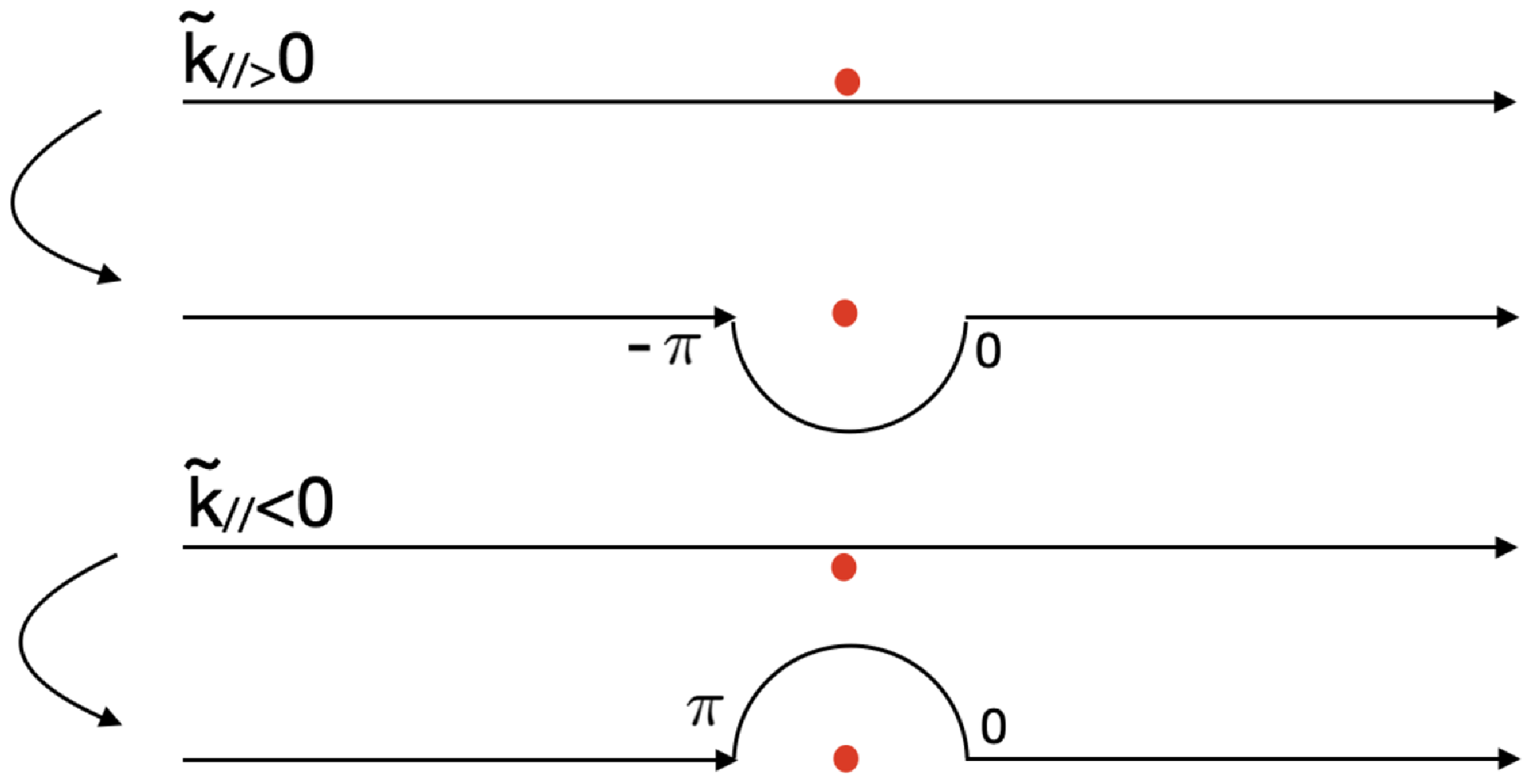
 k~//

 (k⊥,k//,k⊥′,k//′)=(30,7,20,4)/m
 T0,//=7keV
 T0,⊥=7keV
 T0,⊥=112keV
 T0,⊥=700keV

 Open access

