1. Introduction
It is a well-known fact that expectations drive actions and actions affect expectations. This loop generates a two-way feedback: from agents’ expectations to the dynamics of a variable of interest (Feedback 1 hereafter) and from the latter to the formation of expectations (Feedback 2). In standard macroeconomic models, agents hold rational expectations (REs) à la Muth (Reference Muth1961): they know the “true model” of the economy generating Feedback 1 and the stochastic process governing the macroeconomic shocks (Hansen and Sargent, Reference Hansen and Sargent2014) and take the probability distribution of the variable into account. REs therefore are model-consistent and unbiased.Footnote 1
Agents holding adaptive expectations (AEs) base instead their expectations only on the past history of the variable of interest. This is due to limited cognitive capabilities or limited capacity to pay attention to all the information agents have access to (Sims, Reference Sims1998, Reference Sims2003). In the presence of a high degree of “complexity,” agents are likely to rely on simple rules to form expectations because model-consistent expectations are simply too difficult to implement.
Abundant experimental evidence shows that indeed humans do not fully grasp how the market or the macroeconomy work. In fact, “the outcomes of many Learning to Forecast (LtF) laboratory experiments contradict the RE hypothesis” (Anufriev et al. Reference Anufriev, Hommes and Makarewicz2019, p. 1540). In these experiments, participants often adopt simple rules (or heuristics) to form expectations. AE is one of these heuristics. In the lab, however, adaptive agents do not seem to be prone to systematic errors (Colasante et al. Reference Colasante, Palestrini, Russo and Gallegati2017). This may be due to the fact that subjects in the lab follow a modified adaptive rule that mitigates the tendency to repeat errors embedded in the standard adaptive heuristic. Indeed Anufriev et al. (Reference Anufriev, Hommes and Makarewicz2019) show that a trend-extrapolating rule fits the subjects’ forecasts better than the simple adaptive heuristic.
In this paper, we build a stylized agent-based model (ABM) to explore the forecasting capabilities of adaptive agents in a complex economy. In our ABM firms form heterogeneous AEs of inflation to determine the (optimal) scale of activity: the higher the expected inflation, the higher the employment and production. Even in a stationary setting (the Baseline scenario) when firms use the standard adaptive heuristic (Adaptive regime in the following), Monte Carlo simulations show that they are indeed inefficient forecasters: they generally overestimate inflation and produce more than the market can absorb. In the Adaptive regime, the average forecasting error is sizable.
If firms form expectations augmenting the adaptive rule with a Belief Correction term (BCT) that is based on the past change of inflation (Belief Correction (BC) regime), on the contrary, simulations show that the average forecasting error is close to zero, as in the unbiased (rational) equilibrium. Our adaptive rule augmented with a BCT turns out to be a special case of the First-Order Heuristic (FOH)—based on “anchoring and adjustment” à la Kahneman and Tversky (Kahneman, Reference Kahneman2011)—that seems to be widely used by participants in LtF experiments (Heemeijer et al. Reference Heemeijer, Hommes, Sonnemans and Tuinstra2009).
We have also explored a Non-stationary scenario in which the Government charges a tax on sales to finance fundamental research. In this scenario, total factor productivity (TFP) grows driving aggregate economic activity. The forecasting performance of the adaptive heuristic is bound to worsen. According to the output of simulations, in fact, in the Adaptive regime the average forecast error is even bigger than in the Baseline. In the BC regime, on the contrary, even in a non-stationary setting the average error goes down approximately to zero.
In order to capture the inner mechanism of the ABM we then present and discuss a two-dimensional nonlinear macro-dynamic model with homogeneous expectations which can be thought of as the underlying skeleton of the ABM. The first equation describes the price adjustment process according to which inflation is an increasing function of excess demand (as in the ABM) and captures the feedback from expected inflation—which indirectly determines excess demand—to actual inflation (Feedback 1). The second equation is the expectation formation mechanism which features expected inflation as a nonlinear function of past inflation and captures the feedback from actual inflation to expected inflation (Feedback 2). This two-dimensional system is not solvable analytically. We compute numerical solutions using the same parameter values of the ABM. These solutions replicate the results of the ABM surprisingly well: BC mitigates forecasting error to a great extent.
The paper is organized as follows. After a brief review of the literature (Section 2), in Section 3, we present and discuss the ABM. The Baseline scenario will be presented in Section 4. In Section 5, we explore the Non-stationary scenario characterized by the introduction of a sale tax to finance Government expenditure in fundamental research which affects TFP growth. In Section 6, we present and discuss the two-dimensional nonlinear macro-dynamic skeleton of the ABM. Section 7 concludes. In the appendix, we provide numerical approximation of the unbiased equilibrium.
2. A concise review of the literature
This paper contributes to two strands of literature. The first strand focuses on learning and forecasting in complex environments. In this context agents resort to simple heuristics to form expectations, as in Brock and Hommes (Reference Brock and Hommes1997). Heterogeneous expectations and heuristics switching are thoroughly surveyed in Hommes (Reference Hommes2013). This behavioral approach to expectations formation has been adopted also in Behavioural New Keynesian Dynamic Stochastic General Equilibrium (DSGE) models (Branch and McGough, Reference Branch and McGough2018).
Heuristic switching has been put to test in LtF experiments (Assenza et al., Reference Assenza, Bao, Hommes and Massaro2014). Four robust facts stand out starkly from the experimental evidence: (i) subjects use very few heuristics to form expectations (Assenza et al. Reference Assenza, Heemeije, Hommes and Massaro2019), (ii) the adaptive rule features prominently among these heuristics, (iii) if a negative feedback of type 1 is at work—that is, if the current state of the variable is a decreasing function of the average expectation—learning leads to fast monotonic convergence of the variable to the RE equilibrium provided the feedback is linear (in nonlinear cases, the dynamics can be more complicated), and (iv) with positive feedback oscillatory trajectories are more likely and oscillations may be either dampening (ensuring convergence to the RE solution in the long run) or permanent (Heemeijer et al. Reference Heemeijer, Hommes, Sonnemans and Tuinstra2009; Anufriev et al. Reference Anufriev, Hommes and Makarewicz2019).
When the environment is “simple to understand,” also AEs tend to be unbiased. The environment is simple to understand when it is stationary. When the state variable is growing or declining, on the contrary, the environment is difficult to understand and AEs generally fail. Colasante et al. (Reference Colasante, Palestrini, Russo and Gallegati2017) test in the lab whether subjects using an adaptive rule learn the presence of a drift and incorporate this acquired knowledge in expectation formation. It turns out that participants in the experiment are indeed capable of grasping the drift and this improves their forecasting performance to a large extent. Trend-following in expectations formation makes even a dynamic environment understandable to the adaptive agent (Palestrini and Gallegati, Reference Palestrini and Gallegati2015).
Heemeijer et al. (Reference Heemeijer, Hommes, Sonnemans and Tuinstra2009) present an encompassing FOH based on “anchoring and adjustment” that nests all the heuristics actually used by participants in LtF experiments. The scheme of AEs augmented by a BCT used in our ABM is a particular case of this heuristic.
The second strand of literature is agent-based macroeconomics. A large number of agent-based macroeconomic frameworks has been developed over the last two decades: Dawid and Delli Gatti (Reference Dawid, Gatti, Dawid and Gatti2018) provide an extensive survey. In these models, agents are generally assumed to form AEs. Variants and alternatives to the adaptive option to model expectations within this literature are discussed extensively in Salle (Reference Salle2015). For an application of the heuristics switching mechanism to an agent-based macroeconomic framework see Dosi et al. (Reference Dosi, Napoletano, Roventini, Stiglitz and Treibich2017). The aim of our ABM is to show that the bias generated by the adaptive scheme can be mitigated even in complex environments by a BCT.
3. An ABM with heterogeneous expectations
Since we want to explore how BC affects the agents’ forecasting capability, the model we present in this section is much simpler than most of the models reviewed in Dawid and Delli Gatti (Reference Dawid, Gatti, Dawid and Gatti2018). We consider a closed economy populated by households and firms. Households (not explicitly modeled) supply labor, earn wages, and spend on consumption goods their wages entirely (they are “hand to mouth” consumers).
3.1. The optimal scale of activity
Firms produce a homogeneous consumption good. The production function of the i-th firm (
 $i=1,2,\ldots,F$
) is
 \begin{equation} Q_{i,t}=A_t N_{i,t}^{\frac{1}{\delta }} \end{equation}
where
 $Q_i$
and
 $N_i$
are output and employment,
 $A$
is TFP and
 $\delta \gt 1$
. The growth rate of TFP is a random variable whose realizations are
 $g_A\gt 0$
with probability
 $p_A (\tau )$
, zero otherwise. The probability of TFP growth is increasing with the sale tax rate
 $\tau$
. We assume, in fact, that sale taxes finance public investment in fundamental research and fundamental research, in turn, affects success in innovation and TFP growth. For simplicity, we assume
 $p_A=\gamma _{A}\tau$
with
 $\gamma _{A}\gt 0$
. When
 $\tau =0$
, there is no Government expenditure in research and TFP is stationary. We assume
 $A=1$
in this case. The stationarity of TFP characterizes the Baseline scenario that will be presented in section 4. We will discuss the consequences of TFP growth in the Non-stationary scenario of section 5.
Due to labor market “frictions,” the real wage
 $w_{t}$
does not adjust to imbalances between demand and supply of labor but follows an exogenous AR(1) process with drift:
 \begin{equation} w_{t}=\rho _{w}w_{t-1}+d+\sigma _{\varepsilon }\varepsilon _{W} \end{equation}
where
 $d\gt 0$
is the drift,
 $\rho _w\in (0,1)$
is the autoregressive coefficient and
 $\varepsilon _{W}\sim \mathcal{N}(0,\sigma _\varepsilon )$
is a wage shock. We rule out labor shortages. By assumption, labor supply (not modeled) is always abundant.
At the beginning of period
 $t$
, the firm decides the quantity to be produced (and the workers to be employed). Production takes time and output will be available only at the end of the period, when the market for consumption goods opens and transactions are carried out. At the moment it takes decisions, therefore, the firm is uncertain on the sale price
 $P_{t}$
.
Under risk neutrality and perfect competition, the firm chooses at the beginning of t the optimal quantity by maximizing expected profits (net of taxes):
 \begin{equation*} \max _{Q_{i,t}} \Phi _{i,t}^{e}=\pi _{i,t}^{e}(1-\tau )Q_{i,t}-w_{t}{A_t}^{-\delta } Q_{i,t}^\delta \end{equation*}
where
 $\pi _{i,t}^{e}$
is the real price expected by the i-th firm for period
 $t$
, that is, the ratio of the nominal price at which the firm expects to sell its goods
 $P_{i,t}^{e}$
to the aggregate price level. Since the firm does not know
 $P_{t}$
at the moment decisions are taken, the expectation of the real price is based on the aggregate price observed at the end of period
 $t-1$
,
 $P_{t-1}$
. Hence,
 \begin{equation} \pi _{i,t}^{e}\;:\!=\;\frac{P_{i,t}^{e}}{P_{t-1}} \end{equation}
 $\pi _{i,t}^{e}$
turns out to be the gross inflation rate expected by the i-th agent. The solution of this maximization problem yields optimal output:
 \begin{equation} Q_{i,t}=\eta \zeta _t \left (\pi _{i,t}^{e}\right )^{\frac{1}{\delta -1}} \end{equation}
where
 \begin{equation*} \zeta _t\;:\!=\;A_t ^{\frac {\delta }{\delta -1}}w_t ^{-\frac {1}{\delta -1}} \end{equation*}
 \begin{equation*} \eta \;:\!=\;\left (\frac {1-\tau }{\delta }\right )^{\frac {1}{\delta -1}} \end{equation*}
Plugging (4) into (1) and rearranging, we get the demand for labor:
 \begin{equation} N_{i,t}=\frac{1}{w_t}\eta ^\delta \zeta _t \left (\pi _{i,t}^{e}\right ) ^{\frac{\delta }{\delta -1}} \end{equation}
Since
 $\pi _{i,t}^{e}(1-\tau )$
is the expected marginal revenue, output, and employment are increasing with inflation expectations. Firms with relatively “high” inflation expectations (high expected marginal revenue) will produce more than firms holding “low” inflation expectations.
Aggregate demand in real terms is equal to the total wage bill
 $w_t N_t$
where
 $N_t\;:\!=\;\sum _{i=1}^F N_{i,t}$
is total employment. Since firms produce a homogeneous consumption good, we assume that a fraction
 $1/F$
of the wage bill is spent at each firm by each household. Actual sales for the i-th firm (
 $S_{i,t}$
), therefore, may be different from output planned and brought to the market:
 $S_{i,t}=\min (Q_{i,t},\frac{w_t N_{t}}{F})$
.
3.2. Price adjustment
Overall excess demand will be
 $ED_{t}=w_t N_t -Q_t$
where
 $Q_t\;:\!=\;\sum _{i=1}^F Q_{i,t}$
is aggregate supply. If excess demand is positive, all the output will be sold (and there may be a fringe of unsatisfied consumers at some firms). In this case, we assume that the sale price at the end of the period
 $P_{t}$
will be higher than the price carried over from the past. If, on the contrary, excess demand is negative, the end-of-period price will be lower than
 $P_{t-1}$
. However, there is no guarantee of market clearing as we do not assume the presence of a top-down coordinating mechanism such as the auctioneer which brings necessarily demand into equality with supply. On the basis of these consideration, denoting with
 $\pi _{t}\;:\!=\;\frac{P_{t}}{P_{t-1}}$
the gross inflation rate, we assume the following market protocol.
Assumption 1. The market price evolves according to the stochastic adjustment process:
 \begin{equation} \pi _{t}=\exp \left (\gamma _{p}ED_{t}\right )\exp (\varepsilon _{P}) \end{equation}
where
 $\gamma _{p}\gt 0$
,
 $ED_t$
is excess demand:
 \begin{equation} ED_t=w_t \sum _{i=1}^F N_{i,t} -\sum _{i=1}^F Q_{i,t} \end{equation}
and
 $\varepsilon _{P} \sim \mathcal{N}(0,\sigma _\varepsilon )$
is a price shock,
 $E\left (\exp (\varepsilon _{P})\right ) \approx 1$
.
Excess demand is known in t because all the variables involved (total output and the total wage bill) are determined in t on the basis of individual inflation expectations. By construction, when there is market clearing (
 $ED_t=0$
) the price is stationary (
 $\pi _{t}=1$
).Footnote
2
Substituting optimal output and employment into excess demand and the latter into the price adjustment equation (6), we obtain the relationship between expected inflation and actual inflation (Feedback 1) in the ABM:
 \begin{equation} \pi _{t}=\exp \left \{ \gamma _{p}\zeta _t \left [\eta ^\delta \sum _i{(\pi _{i,t}^{e})}^{\frac{\delta }{\delta -1}}-\eta \sum _i{(\pi _{i,t}^{e})}^{\frac{1}{\delta -1}}\right ]\right \}\exp (\varepsilon _{P}) \end{equation}
Actual inflation therefore is a nonlinear function of individual inflation expectations.
3.3. Expectations
We consider two regimes of expectation formation. In the standard Adaptive regime, we assume that agents form expectations of the sale price according to the canonical Cagan–Friedman–Nerlove adaptive algorithm. In the BC regime, they follow an error mitigation strategy which consists in augmenting their adaptive algorithm by a BCT equal to the expected first difference of the price
 $\Delta ^e_{P_t}$
. To encompass both regimes in a general algorithm, we assume the following expectations formation mechanism:
Assumption 2. The i-th agent forms expectations on the sale price at the end of period
 $t$
using the following algorithm:
 \begin{equation} P_{i,t}^{e}=\lambda _{i}P_{t-1}+(1-\lambda _{i})P_{i,t-1}^{e}+\boldsymbol{1}_{P} \Delta _{P_t}^e \end{equation}
where
 $\boldsymbol{1}_{P}$
is an indicator function that takes value 0 in the Adaptive regime and 1 in the BC regime and
 $\Delta _{P_t}^e$
is the expected change of the price level between t-1 and t.
Notice that price expectations are heterogeneous because the expectation updating coefficient
 $\lambda _i$
is firm specific. In the ABM,
 $\lambda _{i}$
is drawn from a uniform distribution with support
 $\left (\lambda _0,1\right ]$
;
 $\lambda _0\gt 0$
. Iterating (9), we get
 \begin{equation} P_{i,t}^{e}=\lambda _{i} \sum _{s=0}^{\infty }(1-\lambda _{i})^s P_{t-s-1} +\boldsymbol{1}_{P} \sum _{s=0}^{\infty }(1-\lambda _{i})^s \Delta _{P_{t-s}}^e \end{equation}
In the simplest setting, the estimated change coincides with the past first difference—that is,
 $\Delta _{P_t}^e=\Delta _{P_{t-1}}\;:\!=\;P_{t-1}-P_{t-2}$
—so that (9) becomes:
 \begin{equation} P_{i,t}^{e}=\lambda _{i}P_{t-1}+(1-\lambda _{i})P_{i,t-1}^{e}+\boldsymbol{1}_{P} (P_{t-1}-P_{t-2}) \end{equation}
When agents adopt a BC strategy (11) may be interpreted as a variant of the so-called FOH put forward by Heemeijer et al. (Reference Heemeijer, Hommes, Sonnemans and Tuinstra2009) to interpret the forecasting behavior of human subjects in LtF experiments. The FOH of agent i is defined as follows:
 \begin{equation} P^e_{i,t}=\lambda _i P_{t-1}+\mu _i P^e_{i,t-1}+(1-\lambda _i-\mu _i)P^*+\gamma _i (P_{t-1}-P_{t-2}) \end{equation}
with
 $\lambda _i$
and
 $\mu _i$
positive and such that
 $\lambda _i +\mu _i \leq 1$
and
 $P^*$
the long-run value of
 $P$
. FOH is an anchoring and adjustment heuristic, that is, a combination of an anchor—consisting of a weighted average of the lagged value of the variable, the lagged expectation and the long-run value—and a trend-extrapolating term proportional to the lagged first difference of the variable.
Experimental evidence shows that the trend parameter
 $\gamma _i$
is positive (but smaller than one) for the majority of participants in LtF experiments in environments with positive feedback. In the case of negative feedback, subjects generally do not extrapolate the trend (
 $\gamma _i=0$
) or—in few cases—act as contrarians (
 $\gamma _i\lt 0$
). In this setting, agents’ learning behavior does not converge in general to REs but points in the direction of behavioral learning equilibria as discussed in Hommes and Zhu (Reference Hommes and Zhu2014).Footnote
3
The algorithm (11) can be conceived as a special case of FOH characterized by
 $\mu _i=1-\lambda _i$
. The anchor is the standard AE algorithm and the trend-extrapolating factor is the BC term. For simplicity we assume that the trend extrapolating parameter is positive, uniform across agents and equal to 1 independently of the sign of the feedback.
Let’s now go back to the expectations formation mechanism (10). Dividing both sides of this equation by
 $P_{t-1}$
we get expected inflation
 \begin{equation} \pi ^e_{i,t}= \bar \pi _{i,t}+\boldsymbol{1}_{P}\overline{\xi }_{i,t} \end{equation}
where
 \begin{equation*}\bar \pi _{i,t}\;:\!=\;\lambda _{i} \sum _{s=0}^{\infty }(1-\lambda _{i})^s \frac {P_{t-1-s}}{P_{t-1}}=\lambda _{i}\left [1+\frac {1-\lambda _i}{\pi _{t-1}}+\frac {(1-\lambda _i)^2}{\pi _{t-2}\pi _{t-1}}\ldots \right ]\end{equation*}
 \begin{equation*} \overline {\xi }_{i,t}\;:\!=\;\sum _{s=0}^{\infty }(1-\lambda _{i})^s \frac {\Delta _{P_{t-s}}^e}{P_{t-1}}=\frac {\Delta _{P_{t}}^e}{P_{t-1}}+(1-\lambda _{i})\frac {\Delta _{P_{t-1}}^e}{P_{t-1}}+\ldots \end{equation*}
Inflation expectations are heterogeneous because firms use different updating coefficients
 $\lambda _i$
.
In the ABM we assume that agents are relatively sophisticated smoothers so that the estimated first difference is the mean of the past four first differences:
 \begin{equation} \Delta _{P_{t-s}}^e=\frac{1}{4}\sum ^4_{z=1} \Delta _{P_{t-s-z}} \end{equation}
Hence the term
 $\overline{\xi }_{i,t}$
can be written as follows:
 \begin{align*} \begin{split} \overline{\xi }_{i,t}:&=\frac{\Delta ^e_{P_t}}{P_{t-1}}+(1-\lambda _{i})\frac{\Delta ^e_{P_{t-1}}}{P_{t-1}}+\ldots \\ &=\frac{1}{4}\left [\left (1-\frac{1}{\pi _{t-1}\ldots \pi _{t-4}}\right )+(1-\lambda _{i})\left (\frac{1}{\pi _{t-1}}-\frac{1}{\pi _{t-1}\pi _{t-2}\ldots \pi _{t-5}}\right )+\ldots \right ] \end{split} \end{align*}
4. The Baseline scenario
In this section, we present and discuss the simulations of the ABM in the Baseline scenario characterized by stationarity. In this scenario, in fact,
 $\tau = 0$
so that there is no investment in fundamental research.Footnote
4
Hence, TFP is constant:
 $A=1$
. The dynamics of the model in the Baseline, therefore, is driven exclusively by the law of motion of the real wage (2). We assume individual expectations are formed adaptively as shown in (13) with the expected change of the price level defined in (14). Therefore, optimal output and employment will be
 \begin{align} Q_{i,t} & =\eta \zeta _t \left (\bar \pi _{i,t}+\boldsymbol{1}_{P}\overline{\xi }_{i,t}\right )^{\frac{1}{\delta -1}} \end{align}
 \begin{align} N_{i,t} & =\frac{1}{w_t}\eta ^\delta \zeta _t \left (\bar \pi _{i,t}+\boldsymbol{1}_{P}\overline{\xi }_{i,t}\right ) ^{\frac{\delta }{\delta -1}} \end{align}
In the Baseline,
 $\zeta _t$
and
 $\eta$
boil down to
 $\zeta _t=w_t ^{-\frac{1}{\delta -1}}$
and
 $\eta =\delta ^{-\frac{1}{\delta -1}}$
.
There are only 8 parameters in this simple model. The numerical values of the parameters used in simulations are gathered in Table 1. We have calibrated
 $\delta$
at 3/2 in order to set the elasticity of output to labor at 2/3. This is in line with the long-run level of the labor share in the USA after the Great Depression. For simplicity this calibration does not incorporate the tendency of the labor share to decline after 1980 highlighted by the recent literature on declining business dynamism. We set the growth rate of the innovation process
 $g_A$
at 0.02 to replicate the average growth rate of the USA.
Parameter values

We have set the numerical values of the other parameters in order to generate dynamic patterns of artificial time series that do not show sudden changes or bifurcations near the chosen numerical values. We performed local sensitivity analysis, given the extreme difficulty of conducting global analyses in these models.
We have chosen the autoregressive coefficient
 $\rho _w$
and the constant
 $d$
in the law of motion of the wage in order to get an average wage (across time periods) equal to 1. The support of the distribution of updating coefficients
 $\lambda _i$
has been limited by setting the lower bound
 $\lambda _0$
at
 $0.4$
in order to ensure that expectations update rapidly enough.
Having set
 $\gamma _P=0.001$
and
 $\delta =3/2$
, we get
 $\zeta _t=w_t^{-2}$
,
 $\eta =\delta ^{-2}=4/9$
and
 $\eta ^\delta =\delta ^{-3}=8/27$
. Using these numerical values, we retrieve optimal output and employment from (15) and (16). Substituting the resulting expressions into excess demand (7) and the latter into (6), we obtain the following Feedback 1 in the Baseline scenario:
 \begin{equation} \pi _{t}=\exp \left \{\frac{0.001}{w_t ^{2}} \left [\frac{8}{27} \sum _i{\left (\bar \pi _{i,t}+\boldsymbol{1}_{P}\overline{\xi }_{i,t}\right )}^{3} -\frac{4}{9} \sum _i{\left (\bar \pi _{i,t}+\boldsymbol{1}_{P}\overline{\xi }_{i,t}\right )}^{2}\right ]\right \} \exp (\varepsilon _{P}) \end{equation}
Actual inflation is a nonlinear function of individual inflation expectations—that in turn are functions of past inflation—and of the wage rate, that is determined by the AR(1) stochastic process.
We run
 $S=100$
Monte Carlo simulations of the ABM (with different random seeds). The duration of each simulation is
 $T=40$
periods. Hence, each individual expectation
 $\pi ^e_{i,t,s}$
is characterized by three indices:
 $i=1,2,\ldots F$
,
 $t=1,2,\ldots T$
,
 $s=1,2,\ldots S$
. Simulation
 $s$
generates in period
 $t$
the distribution of
 $F=200$
individual inflation expectations
 $\pi ^e_{i,t,s}$
, which in turn will generate actual inflation
 $\pi _{t,s}$
through (17). For each simulation
 $s$
, we retrieve the “long-run” distribution of individual inflation expectations, that is, the distribution of expectations in the final period:
 $\pi ^e_{i,T,s}$
,
 $i=1,2,\ldots F$
. The long-run average expectation (i.e., inflation expected on average by the population of firms in period
 $T$
) is the mean of the long-run distribution of expectations:
 \begin{equation} \pi _{T,s}^{e}=\frac{\sum _{i=1}^F \pi ^e_{i,T,s}}{F} \end{equation}
The actual long-run inflation associated to simulation
 $s$
is inflation of the last period
 $\pi _{T,s}$
. The difference between actual and expected inflation (both referred to period
 $T$
) is the forecast error associated to simulation
 $s$
:
 $\varepsilon _{T,s}=\pi _{T,s}-\pi _{T,s}^{e}$
. Finally, the bias is the percent forecast error in the last period:
 $b_{T,s}=\frac{\pi _{T,s}}{\pi ^e_{T,s}}-1$
. The bias distribution is the distribution of
 $S=100$
biases (one for each simulation). We evaluate the performance in forecasting of the population of firms by means of the first and second moments of the bias distribution, that is, the average bias
 \begin{equation} b=\frac{\sum _{s=1}^{S} b_{T,s}}{S} \end{equation}
and the variance of the bias:
 \begin{equation} \sigma ^2_b=\frac{\sum _{s=1}^{S} (b_{T,s}-b)^2}{S} \end{equation}
By construction, when expectations are unbiased the bias is zero. In the appendix, we develop the unbiased benchmark: we consider an economy populated by identical firms that know the true model of the economy, that is, the equation for Feedback 1 (equation (8)) calibrated with the same numerical parameters used for the ABM. In this setting, it is straightforward to show that when expectations are rational, the forecast error is
 $\varepsilon _t=E(\pi _t)[\exp (\varepsilon _{P})-1]$
and the bias is
 $b_t=\exp (\varepsilon _{P})-1$
so that the expected value of the bias is zero. In words, model-consistent expectations are unbiased. This allows to measure the departure of the bias generated by the ABM from the unbiased solution.
From simulations of the ABM in the Baseline scenario, we get the following fundamental result:
Result 1. In the Adaptive regime, the average bias is significantly different from zero:
 $b=-2.5\%$
, that is, agents overestimate inflation by a non-negligible margin. Moreover, the standard deviation of the bias (
 $\sigma _b=0.012$
) is slightly bigger than the standard deviation of the price shock.
Footnote
5
On the contrary, in the BC regime, the average bias
 $b'\approx 0$
, while the standard deviation of the bias does not change.
Let’s now turn to output and employment. Each simulation generates the time series of total output
 $Q_{t,s}=\sum ^F_{i=1} Q_{i,t,s}=\eta \zeta _t \sum ^F_{i=1} \left (\bar \pi _{i,t,s}+\boldsymbol{1}_{P}\overline{\xi }_{i,t,s}\right )^{\frac{1}{\delta -1}}$
and of total employment
 $N_{t,s}=\sum ^F_{i=1} N_{i,t,s}=\frac{1}{w_t}\eta ^\delta \zeta _t \sum ^F_{i=1}\left (\bar \pi _{i,t,s}+\boldsymbol{1}_{P}\overline{\xi }_{i,t,s}\right ) ^{\frac{\delta }{\delta -1}}$
,
 $t=1,2,\ldots T$
.
In the appendix, we retrieve employment in the unbiased case plugging the RE of inflation in the equation for optimal employment. We denote employment when expectations are unbiased in the Baseline with
 $N^{UB}$
. In the Rational Representative Agent setting, agents know the AR(1) process governing the evolution of the wage rate and can therefore determine the long-run value of the wage
 $w_{T}$
. Each Monte Carlo simulation generates a different final period wage
 $w_{T,s}$
,
 $s=1,2,\ldots 100$
. Therefore, we determine the (long-run) unbiased solution for employment
 $N^{UB}_{T,s}$
for each simulation. We define the employment ratio as the ratio of long-run employment
 $N_{T,s}$
generated by the ABM in simulation s to employment when expectations are unbiased in the same simulation. In this way, we generate the distribution of employment ratios:
 $\nu _s\;:\!=\;\frac{N_{T,s}}{N^{UB}_{T,s}}$
,
 $s=1,2,\ldots 100$
. The mean of this distribution
 $\nu =\sum ^S_{s=1}\nu _s/S$
—that is, the average employment ratio—is a measure of over- or under-employment relative to the unbiased case. From simulations we get the following fundamental result:
Result 2. In the Adaptive regime the average employment ratio is
 $\nu =1.08$
, that is, employment is 8% bigger than in the unbiased case. In the BC regime, on the contrary, the average employment ratio is
 $\nu '=0.997$
, that is, the distribution is centered around 1: employment is approximately the same as in the unbiased case.
The rationale for Result 2 is the following. In our simulations, given the initial conditions, if firms do not apply BC, on average inflation expectations converge to a “long-run” level
 $\pi _t^e$
that significantly overestimates actual inflation
 $\pi _T$
(the bias is negative, as stated in Result 1). Therefore, firms optimally employ a larger number of workers and produce more than in the unbiased case. If, on the contrary, they apply BC, on average firms do not overestimate actual inflation so that employment and production are approximately the same as in the unbiased case.
5. Non-stationary scenario
In this section, we explore the Non-stationary scenario generated by active fiscal policy and public investment in fundamental research. In this scenario, in fact, the Government finances expenditure in R&D by charging a proportional tax on sales. The tax rate is
 $\tau =0.05$
. Given the parameter values used in simulations (see Table 1), the probability of TFP growth in this scenario is
 $p_A=\gamma _\tau \tau =0.2$
. We set TFP growth in case of success of the policy at
 $g_A=0.02$
. In this scenario, GDP grows over time generating a non-stationary setting in which agents must form expectations. We run 100 Monte Carlo simulations of the ABM in the Non-stationary scenario. As in the Baseline, the time span of each simulation is 40 periods. Each simulation generates a distribution of
 $F=200$
inflation expectations for each period (as shown above). Following the procedure outlined above for the Baseline scenario, we can compute actual inflation in period
 $T=40$
, average expected inflation and the associated bias. In this way, we generate the distribution of
 $S=100$
biases, denoted with
 $b^N_{T,s}$
. Hence, the average bias in the Non-stationary scenario is
 $b_N=\frac{\sum _{s=1}^{S} b^N_{T,s}}{S}$
.
In Figure 1, we show the bias distribution in the Non-stationary scenario with canonical AEs and with BC. In the unbiased benchmark (see appendix), the equation for Feedback 1 is affected by the TFP shock and therefore also the unbiased solution for inflation will change but, assuming that the representative agent knows the true model of the economy and the properties of the shocks, the expected value of the bias is still zero. In words, model-consistent expectations are unbiased also in the Non-stationary scenario.
Distribution of the bias
 $b^N_{T,s}$
,
 $s=1,2,\ldots 100$
in the Non-stationary scenario. The probability density function of the bias is generated by means of kernel density estimation (bandwidth: 0.148). The left (blue in the online version) density is generated in the Adaptive regime, the right (red online) density is obtained in the Belief Correction regime. For the color version of the figures, we refer to the online version of this paper.

We can summarize the results of these simulations as follows:
Result 3. In the Adaptive regime, the mean of the bias distribution is
 $b_N=-4\%$
and the standard deviation is
 $\sigma _N=0.0224$
. Firms overestimate inflation in the Non-stationary scenario more than in the Baseline scenario. In the BC regime, the mean of the bias goes down approximately to
 $b'_N=0.5\%$
and the standard deviation falls to
 $\sigma '_N=0.0127$
.
Also in the Non-stationary scenario we compute the employment ratio
 $\nu ^N_{T,s}\;:\!=\;\frac{N^N_{T,s}}{N^{UN}_{T,s}}$
,
 $s=1$
,
 $2,\ldots 100$
as the ratio of long-run employment
 $N^N_{T,s}$
generated by the ABM in simulation s of the Non-stationary scenario to employment when expectations are unbiased
 $N^{UN}_{T,s}$
in the same simulation. The mean of this distribution
 $\nu _N=\sum ^S_{s=1}\nu _{s}/S$
is the average employment ratio in this scenario. Figure 2 shows the distribution of the employment ratio in the Non-stationary scenario.
Result 4. In the Adaptive regime the average employment ratio is
 $\nu _N=1.14$
, that is, employment is 14% bigger than in the unbiased case. The employment ratio is bigger than in the Baseline. In the BC regime, on the contrary, the average employment ratio is
 $\nu '_N=0.990$
, that is, employment is approximately the same as in the unbiased case.
Distribution of the employment ratio
 $\nu ^N_{T,s}$
in the Non-stationary scenario. The probability density function of the employment ratio is generated by means of kernel density estimation (bandwidth: 0.003). The left (blue online) density is generated in the Adaptive regime, the right (red online) density is obtained in the Belief Correction regime.

We can further assess the effects of BC in a Non-stationary environment by tracking the evolution over time of the dynamic employment ratio
 $\psi _t=\frac{N^N_t}{N_t}$
, that is, the ratio of aggregate employment in the Non-stationary scenario to aggregate employment in the stationary Baseline (when expectations incorporate the BCT). The numerator of this ratio grows over time while the denominator is stationary, causing the ratio to increase at the same rate of the numerator. Notice that since TFP is growing over time, also aggregate employment in the unbiased case is growing in the Non-stationary scenario while it is stationary in the baseline. Therefore, the employment ratio
 $\psi ^U_t=\frac{N^{UN}_t}{N^{UB}_t}$
grows at the same rate of the numerator. Employment in the unbiased case in the Non-stationary scenario grows approximately at the rate:
 \begin{equation} g^{UN}=(1-p_A) + p_A (1+g_A)^{\frac{\delta }{\delta -1}}-1. \end{equation}
Since we have set
 $p_A=0.2; g_A=0.02$
and
 $\delta =1.5$
, the unbiased case implies a growth rate of employment approximately equal to 1.2% per period.
Figure 3 plots the time series of
 $\psi _{t}$
. The TFP shock generates a jump process. Note that in the initial interval (until period 6 included)
 $\psi \lt 1$
because the introduction of a sale tax has a direct negative effect on marginal revenue, employment, and output. From period 7 onward,
 $\psi$
becomes greater than one and increases steadily over time due to the increase in TFP and the associated decline of marginal cost. It goes from
 $\psi _1=0.8576$
in period 1 to
 $\psi _{36}=1.608$
at the end of the simulation window.Footnote
6
This implies an average (net) rate of employment growth equal to
 $(1.608/0.8676)^{1/36} = 1.0173$
. The fact that the rate of growth of employment in the ABM is close to the unbiased solution is robust across simulations. The Monte Carlo analysis shows a mean rate of growth equal to
 $1.2085\%$
with standard deviation
 $13.5782\%$
. This leads to the final result.
Result 5. The rate of growth in employment generated by the ABM in the Non-stationary scenario and BC regime has the same order of magnitude of the growth in employment in the unbiased case.
Evolution of
 $\psi _t$
. The stars represent
 $\psi$
at each period of the time interval explored with simulations.

This is an intriguing result. The rationale can be described as follows. Contrary to adaptive agents, agents holding unbiased expectations correctly anticipate the average profit function. This implies that initial levels of economic activity may be different in the unbiased case and in the ABM. But when TFP growth makes the profit function shift, adaptive agents that implement BC tend to follow the evolution of the distribution of profits more or less in line with rational agents.
6. Anatomy of the ABM
In the ABM, the feedback from inflation expectations to current inflation (Feedback 1, denoted with
 $FB_1$
) is described by the price adjustment equation (8) while the feedback from past inflation to expectations (Feedback 2, denoted with
 $FB_2$
) is described by the expectation formation equation (13). Hence, in the end, the ABM boils down to the dynamical system
 \begin{equation} D: \begin{cases} \pi _{t}=\exp \left \{ \gamma _{p}\zeta _t \left [\eta ^\delta \sum _i{(\pi _{i,t}^{e})}^{\frac{\delta }{\delta -1}}-\eta \sum _i{(\pi _{i,t}^{e})}^{\frac{1}{\delta -1}}\right ]\right \}\exp (\varepsilon _{P})\\[5pt] \pi _{i,t}^{e}=\bar \pi _{i,t}+\textbf{1}_P\overline{\xi }_{i,t} \ \text{i=1,2},\ldots \text{F} \end{cases} \end{equation}
where both
 $\bar \pi _{i,t}$
and
 $\overline{\xi }_{i,t}$
are functions of past inflation. In order to bring to the fore the interaction between expected inflation and actual inflation in the ABM, in this section, we present and discuss a simplified version of system D which can be conceived as the “skeleton” of the ABM.
6.1. Reinterpreting the price adjustment process
In the price adjustment equation, aggregate demand and supply are proportional to the sum of (individual) inflation expectations raised to the power of
 $\frac{\delta }{\delta -1}$
and
 $\frac{1}{\delta -1}$
, respectively. In our calibration of the ABM (see Table 1),
 $\delta =3/2$
. Hence, aggregate demand and supply are proportional to the sum of cubed and squared inflation expectations, respectively.
By definition, the raw moment of order
 $k$
of the distribution of heterogeneous expectations is
 $m_{k,t}\;:\!=\;\frac{\sum ^F_{i=1}{(\pi _{i,t}^{e})}^k}{F}$
so that
 $\pi _t^e=\frac{\sum _{i=1}^F \pi _{i,t}^{e}}{F}=m_{1,t}$
is the mean of the distribution, that is, the average expectation. Therefore, we can write
 $\sum ^F_{i=1} (\pi _{i,t}^{e})^k=F m_{k,t}$
and
 $FB_1$
becomes
 \begin{equation} \pi _{t}=\exp \left \{ \gamma _{p}\zeta _t F\left (\eta ^\delta m_{3,t}-\eta m_{2,t}\right )\right \}\exp (\varepsilon _{P}) \end{equation}
Let’s denote the central moment of order
 $k$
of the distribution with
 $\sigma _{k,t}=\frac{\sum ^F_{i=1}{(\pi _{i,t}^{e}-\pi _t^e)}^k}{F}$
. Thanks to the algebra of the relationships between raw and central moments, we can rewrite (23) as follows:Footnote
7
 \begin{equation} \pi _{t}=\exp \left \{ \gamma _{p}\zeta _t F \left [\eta ^\delta \left (\sigma _{3,t}+3\sigma _{2,t} \pi _t^e+(\pi _t^e)^3\right )-\eta \left (\sigma _{2,t}+(\pi _t^e)^2\right )\right ]\right \}\exp (\varepsilon _{P}) \end{equation}
In order to simplify the analysis, in this section, we assume that the updating coefficient
 $\lambda$
is uniform across agents, so that all the agents form the same expectation. Therefore,
 $\sigma _{3,t}=\sigma _{2,t}=0$
 $\forall t$
. To simplify matters further, we shut off the wage shock (so that the real wage goes to
 $\bar w=1$
) and the price shock. Therefore,
 $\zeta _t=A^{\frac{\delta }{\delta -1}}_t=A_t^3$
. In our calibration (see Table 1),
 $\gamma _P=0.001$
and
 $F=200$
. Therefore, in this skeletal model, inflation is a cubic function of the expectation held by the representative agent:
 \begin{equation} \pi _{t}=\exp \left \{0.2\ \zeta _t\left [\eta ^\delta (\pi _t^e)^3-\eta (\pi _t^e)^2\right ]\right \} \end{equation}
The expression in curly braces approximates the inflation rate (i.e., the percent change of the price level). The expression in brackets multiplied by
 $\zeta _t$
is excess demand per firm. Since the wage rate is normalized to unity, the wage bill (and therefore aggregate demand) coincides with employment. In this section, firms are identical. We will denote with
 $n$
and
 $q$
employment and output per firm. Given the parameter values adopted in our calibration,
 $n=\eta ^\delta \zeta _t(\pi _t^e)^3$
and
 $q=\eta \zeta _t(\pi _t^e)^2$
. By construction, therefore, market clearing occurs when
 $n=q$
, that is, when expected inflation is
 $\pi ^e_M=\eta ^{1-\delta }$
. The market clearing level of expected inflation is affected by the sale tax but does not depend on TFP. The levels of optimal output and employment, however, are increasing with TFP. There will be excess supply whenever
 $n\lt q$
, that is, for
 $\pi _t^e\lt \pi ^e_M$
.
We consider first the Baseline scenario characterized by
 $\tau =0$
(so that
 $A=1$
). In the Baseline,
 $\zeta =1$
,
 $\eta =\delta ^{-2}=4/9$
, and
 $\eta ^\delta =\delta ^{-3}=8/27$
. Therefore,
 $FB_1$
specializes to
 \begin{equation} \pi _{t}=\exp \left \{0.2 \left [\frac{8}{27} (\pi _t^e)^3-\frac{4}{9} (\pi _t^e)^2\right ]\right \} \end{equation}
 $FB_1$
is represented by the red line in Figure 4. The dashed red line represents the expression in brackets, that is, excess demand (per firm). The blue line is the 45-degree line.
Feedback 1 and excess demand in the Baseline scenario. The flat curve (red online)represents
 $FB_1$
. The dashed curve represents excess demand (per firm). The slope one line is the 45-degree line.

Point
 $M$
is the market clearing solution, which occurs when the excess demand (dashed red) line cuts the x-axis. Market clearing occurs when
 $\pi ^e_M=\delta =1.5$
(so that
 $q_{M}=n_{M}=1$
), that is, when agents expect the sale price to be (much) greater than the initial price: expectations in equilibrium are not correct. In fact,
 $M$
lies on
 $FB_1$
but does not lie on the 45-degree line.Footnote
8
By construction, the unbiased solutions are the intersections between
 $FB_1$
and the 45-degree line. In the first quadrant, there are two fixed points, one of which characterized by excess supply and deflation (
 $U_B$
) and the other by excess demand and inflation (not shown).Footnote
9
With our calibration, we get
 $\pi ^{UB}=0.9708768$
. In the unbiased solution
 $U_B$
, we get
 $n^{UB}=0.2711555$
and
 $q^{UB}=0.4189341$
. Hence, the unbiased solution is characterized by excess supply and deflation. The unbiased solutions for inflation and employment are reported in the first and second rows of Table 2, first column.Footnote
10
Key numerical results

6.2. Reinterpreting the expectations formation mechanism
Let’s consider now the expectation formation mechanism. In order to simplify matters we assume that the information set available to the representative firm is limited to the price levels in the previous two periods—that is,
 $\Omega _{t}=(P_{t-1}, P_{t-2})$
—and we postulate that in the Adaptive regime the expectation of the price level in t is
 \begin{equation} P^e_t=\lambda P_{t-1}+(1-\lambda )P_{t-2} \end{equation}
We assume, moreover, that the BCT is
 $BCT=P_{t-1}-P_{t-2}$
. Hence, the expectation of the price level in t in the BC regime is
 \begin{equation} P^c_t=(1+\lambda )P_{t-1}-\lambda P_{t-2} \end{equation}
Dividing both sides of these equations by
 $P_{t-1}$
we get
 $\pi _t^e=\lambda +\frac{1-\lambda }{\pi _{t-1}}$
and
 $\pi ^c_t= 1+\lambda -\frac{\lambda }{\pi _{t-1}}$
, respectively. In the ABM, we set the average updating coefficient in the proximity of
 $\lambda =0.8$
. Therefore, in the following, we parameterize inflation expectations as follows:
 \begin{align} \pi _t^e & =0.8+\frac{0.2}{\pi _{t-1}} \end{align}
 \begin{align} \pi ^c_t & = 1.8-\frac{0.8}{\pi _{t-1}} \end{align}
These equations will be referred to as
 $FB_2$
and
 $FB^c_2$
, respectively, since they describe the feedback from past inflation to expected inflation in the two regimes. Notice that in the Adaptive regime expected inflation in t is decreasing with inflation in t-1. In the BC regime, instead, expected inflation is an increasing function of past inflation.
6.3. Inflation dynamics
Consider first the Baseline scenario. The dynamical skeleton of the ABM consists of
 $FB_1$
and
 $FB_2$
:
 \begin{equation} D_0: \begin{cases} \pi _{t}=\exp \left \{0.2\left [\frac{8}{27} (\pi _t^e)^3-\frac{4}{9} (\pi _t^e)^2\right ]\right \}\\[3pt] x^e_{t}=0.8+\frac{0.2}{\pi _{t-1}} \end{cases} \end{equation}
Substituting the second equation in the first one we get the law of motion of inflation:
 \begin{equation} \pi _{t}=\exp \left \{0.2\left [\frac{8}{27} \left (0.8+\frac{0.2}{\pi _{t-1}}\right )^3-\frac{4}{9} \left (0.8+\frac{0.2}{\pi _{t-1}}\right )^2\right ]\right \} \end{equation}
The phase diagram of the nonlinear first-order difference equation (32) is represented by the red curve (labeled
 $LM$
) in Figure 5 (when we measure
 $\pi _t$
on the y-axis).
Baseline: Inflation dynamics in the Adaptive regime. The solid (red online) curve labeled
 $LM$
is the phase diagram of (32). The blue (online version) line is again the 45-degree line (when we measure
 $\pi _t$
on the y-axis). The dashed curve labeled
 $FB_2$
represents Feedback 2 in the Adaptive regime (when we measure
 $\pi _t^e$
on the y-axis). The length of the black vertical segment measures the magnitude of the forecasting mistake.

The blue (online version) line is the 45-degree line. Point
 $S_0$
is the steady state characterized by
 $\pi _0=0.9708816\lt 1$
: in the steady state the price level declines exponentially. In the same figure, we have also plotted point
 $M$
. All the points of
 $LM$
below
 $M$
are characterized by excess supply. The dashed red curve represents
 $FB_2$
when we measure
 $\pi _t^e$
on the y-axis. The coordinate on the y-axis of point
 $E_0$
—that is,
 $\pi ^e_0=1.0059983$
—is expected inflation when the economy is in the steady state (long-run expected inflation). Agents overestimate inflation: they expect the price level to rise while it is actually declining. The forecasting mistake is negative, and its absolute value is the length of the
 $E_0-S_0$
segment. The bias is
 $b=-0.035$
.
Consider now the Baseline scenario in the BC regime. The dynamical model consists of
 $FB_1$
and
 $FB^c_2$
.
 \begin{equation} D_1: \begin{cases} \pi _{t}=\exp \left \{0.2\left [\frac{8}{27} (\pi _t^c)^3-\frac{4}{9} (\pi _t^c)^2\right ]\right \}\\[3pt] x^c_{t}=1.8 -\frac{0.8}{\pi _{t-1}} \end{cases} \end{equation}
Substituting the second equation in the first one we get
 \begin{equation} \pi _{t}=\exp \left \{0.2\left [\frac{8}{27} \left (1.8 -\frac{0.8}{\pi _{t-1}}\right )^3-\frac{4}{9} \left (1.8 -\frac{0.8}{\pi _{t-1}}\right )^2\right ]\right \} \end{equation}
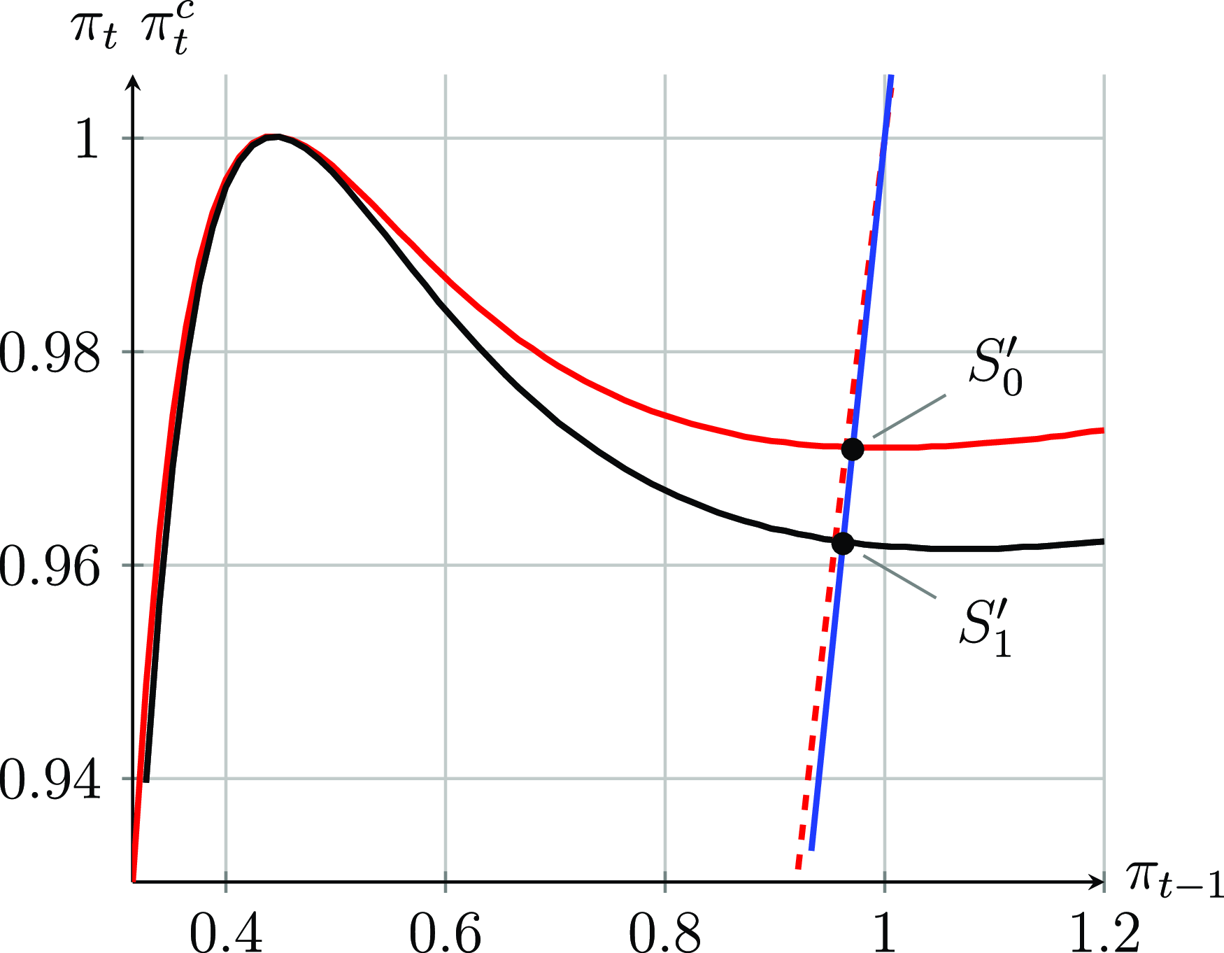
The phase diagram of (34) is represented by the
 $LM'$
curve in Figure 6. Notice that the axes are scaled exactly as in Figure 5.
Baseline: Inflation dynamics in the BC regime. The solid (red online) curve labeled
 $LM'$
is the phase diagram of (34). The blue line is the 45-degree line (when we measure
 $\pi _t$
on the y-axis). The dashed (red online) curve labeled
 $FB^c_2$
represents Feedback 2 in the presence of BC (when we measure
 $\pi _t^e$
on the y-axis).

Point
 $S'_0$
is the steady state, characterized by
 $\pi '_0=0.9708540\lt 1$
. The dashed red line that represents
 $FB^c_2$
(when we measure
 $\pi _t^e$
on the y-axis) is almost undistinguishable from the 45-degree line in the portion of the domain considered in the figure. A closer look shows that expected inflation in the steady state is still higher than current inflation but very close to it:
 $\pi ^c_{0}=0.9759832$
. In the BC regime, the bias is
 $b'=-0.005$
.
We summarize these numerical solutions in the following result.
Result 6. In the Adaptive regime, agents overestimate inflation and the bias is significantly different from zero:
 $b=-3.5\%$
. In the BC regime, the bias shrinks remarkably and is close to zero:
 $b'=-0.5\%$
Agents still overestimate inflation but, thanks to BC, they (i) are correctly expecting the price level to decline and (ii) they are “almost” correct.
This result is in line with result 1 obtained from simulations of the ABM. In the ABM, the average bias (mean of the distribution of individual biases) is −2.5% in the Adaptive regime and is very close to zero in the BC regime. The skeletal model of this section replicates the tendency of the bias to shrink dramatically when agents adopt BC, but the magnitude of the bias is slightly bigger than in the ABM.Footnote 11
Let’s now turn to employment and output. From the numerical solutions, we infer that, in the Adaptive regime (system
 $D_0$
), in the steady state, employment at each firm is
 $n_0=0.3015895$
and the employment ratio is
 $\nu =1.1122$
. In the BC regime (system
 $D_1$
), in the steady state employment is
 $n'_0=0.2754566$
and the employment ratio is
 $\nu '=1.0158$
.
Result 7. In the Adaptive regime employment in the long run is 11.2% greater than in the unbiased solution. Therefore, (i) firms produce more than they would if they correctly anticipated actual inflation, (ii) production is greater than the wage bill so that supply exceeds demand. In the BC regime, instead, employment in the long run is only 1.6% greater than in the unbiased solution. Firms are still overproducing but much less than in the Adaptive regime.
This result aligns with result 2 obtained from simulations of the ABM. In the ABM, in the Adaptive regime employment is 8% bigger than in the unbiased case; in the BC regime, employment is slightly smaller but very close to employment in the unbiased case. The skeletal model replicates fairly well the tendency of the employment ratio to shrink when agents adopt BC, but the magnitude of the employment ratio is slightly bigger than in the ABM. The long-run levels of inflation, expected inflation, the bias, employment, excess demand and the employment rate in the Baseline scenario are reported in the first column of Table 2, starting from the third row.
6.4. Non-stationary scenario
In this section, we consider a Non-stationary scenario characterized by the following assumption: the Government imposes a 5% tax on sales (
 $\tau =0.05$
) and uses the tax revenue to finance
 $R\& D$
that makes TFP jump with certainty and permanently from
 $A_0=1$
(Baseline) to
 $A_1=1.1$
.Footnote
12
The TFP shock therefore makes
 $\zeta$
increase from
 $\zeta _0=1$
(Baseline) to
 $\zeta _1=1.331$
. In the Non-stationary scenario,
 $\eta =0.95^2\times (4/9)$
and
 $\eta ^\delta =0.95^3\times 8/27$
so that
 $FB_1$
specializes to
 \begin{equation} \pi _{t}=\exp \left \{0.2\times 1.331 \left [0.95^3\frac{8}{27} (\pi _t^e)^3-0.95^2\frac{4}{9} (\pi _t^e)^2\right ]\right \} \end{equation}
Market clearing occurs when expected inflation is
 $\pi _M^e=\frac{\delta }{1-\tau }=1.5789$
. There will be excess supply for any
 $\pi _t^e\lt \pi _M^e$
.
 $FB_1$
in the Baseline (i.e., when TFP is
 $A_0=1$
) is represented by the red line in Figure 7 while
 $FB_1$
when TFP is
 $A_1=1.1$
—denoted with
 $FB_1(A_1)$
—is represented by the black line. In blue the 45-degree line.
Feedback 1: effects of a TFP shock. The red line (online version) is
 $FB_1$
in the Baseline (i.e., when TFP is
 $A_0=1$
) while the black line is
 $FB_1$
when TFP is
 $A_1=1.1$
. In blue, again, the 45-degree line.

Points
 $U_B$
and
 $U_N$
are the unbiased solutions in the Baseline and in the Non-stationary scenario. With our calibration, we get
 $\pi ^{UB}=0.9708768$
and
 $\pi ^{UN}=0.9621235$
. The increase in TFP therefore makes inflation go down in the unbiased case. This is confirmed by the numerical solution for the case of a Non-stationary scenario characterized by the same sale tax but a bigger TFP increase (
 $A_1=2$
), as shown by the first row of Table 2.
The dynamical model in the Non-stationary scenario in the Adaptive regime consists of
 $FB_1 (A_1)$
and
 $FB_2$
:
 \begin{equation} D_2: \begin{cases} \pi _{t}=\exp \left \{0.2\times 1.331\left [0.95^3\frac{8}{27} (\pi _t^e)^3-0.95^2\frac{4}{9} (\pi _t^e)^2\right ]\right \}\\[3pt] x^e_{t}=0.8+\frac{0.2}{\pi _{t-1}} \end{cases} \end{equation}
Therefore, the law of motion of inflation becomes
 \begin{equation} \pi _{t}=\exp \left \{0.2\times 1.331\left [0.95^3\frac{8}{27} \left (0.8+\frac{0.2}{\pi _{t-1}}\right )^3-0.95^2\frac{4}{9} \left (0.8+\frac{0.2}{\pi _{t-1}}\right )^2\right ]\right \} \end{equation}
The phase diagram of (37) is represented by the black curve in Figure 8 (when we measure
 $\pi _t$
on the y-axis). To facilitate comparison, the red line is the phase diagram of the law of motion in the Baseline, that is, equation (32).
Inflation dynamics in the Adaptive regime: Effects of a TFP shock. The solid black curve is the phase diagram of (37). The solid above red curve (online version) is the phase diagram of (32). The blue straight line is the 45-degree line (when we measure
 $\pi _t$
on the y-axis). The dashed red curve is
 $FB_2$
in the Adaptive regime (when we measure
 $\pi _t^e$
on the y-axis). The length of the red vertical segment
 $E_0-S_0$
represents the forecasting mistake before the TFP shock. The length of the black vertical segment
 $E_1-S_1$
represents the forecasting mistake after the TFP shock.

The blue line is the 45-degree line. Points
 $S_0$
and
 $S_1$
are the steady states in the Baseline and the Non-stationary scenario, respectively. In the Non-stationary scenario, long-run inflation is slightly smaller than in the Baseline. The increase in TFP therefore exacerbates the deflationary trend. This is confirmed by the numerical solution for the case of a bigger TFP shock (
 $A_1=2$
), as shown by the third row of Table 2.
The dashed red curve represents
 $FB_2$
when we measure
 $\pi _t^e$
on the y-axis. The coordinate on the y-axis of point
 $E_0$
(resp:
 $E_1$
) is expected inflation when the economy is in the steady state
 $S_0$
(
 $S_1$
). Expected inflation is increasing with TFP (see fourth row of Table 2). The forecasting mistake is negative and its absolute value is the length of the
 $E_0-S_0$
segment in the Baseline and of the
 $E_1-S_1$
segment in the Non-stationary scenario. The bias is negative and increasing with TFP (see fifth row of Table 2).
Consider now the Non-stationary scenario in the BC regime. The dynamical model consists of
 $FB_1(A_1)$
and
 $FB^c_2$
:
 \begin{equation} D_3: \begin{cases} \pi _{t}=\exp \left \{0.2\times 1.331\left [0.95^3\frac{8}{27} (\pi _t^e)^3-0.95^2\frac{4}{9} (\pi _t^e)^2\right ]\right \}\\[3pt] x^e_{t}=1.8-\frac{0.8}{\pi _{t-1}} \end{cases} \end{equation}
The law of motion of inflation is
 \begin{equation} \pi _{t}=\exp \left \{0.2\times 1.331\left [0.95^3\frac{8}{27} \left (1.8-\frac{0.8}{\pi _{t-1}}\right )^3-0.95^2\frac{4}{9} \left (1.8-\frac{0.8}{\pi _{t-1}}\right )^2\right ]\right \} \end{equation}
The phase diagram of (39) is represented by the black curve in Figure 9. The red line is the phase diagram of the law of motion in the BC regime in the Baseline (i.e., equation (34)). In blue, the 45-degree line.


Points
 $S'_0$
and
 $S'_1$
are the steady states in the Baseline and the Non-stationary scenario, respectively. In the Non-stationary scenario, steady state inflation is slightly smaller than inflation in the Baseline. Also with BC, therefore, the increase in TFP exacerbates the deflationary trend (see the ninth row of Table 2). The dashed red line represents
 $FB^c_2$
(when we measure
 $\pi _t^e$
on the y-axis). In the Non-stationary scenario (as in the Baseline), expected inflation is still higher than current inflation but very close so that the bias is very close to zero. This is true also for a much bigger TFP shock as shown by row 11 of Table 2.
Given our parameterization, the increase in TFP makes inflation decrease in both regimes. In fact, TFP (one of the determinants of
 $\zeta$
) acts as a magnifier of excess demand in the price adjustment equation. Starting from a long-run situation of excess supply such as
 $S_0$
or
 $S'_0$
, a positive TFP shock amplifies excess supply and therefore contributes to depress the dynamics of the price level.
In the Adaptive regime, the TFP shock magnifies the forecasting mistake because (i) a positive TFP shock makes actual inflation go down and (ii) the decline of actual inflation makes expected inflation go up. On the contrary, in the BC regime, the forecasting mistake shrinks remarkably. In fact, with BC, expected inflation is increasing with actual inflation so that expected inflation fall more or less in line with actual inflation.
We summarize these numerical solutions in the following result:
Result 8. In the Adaptive regime, the magnitude of the bias is increasing with TFP; it goes from
 $b=-3.5\%$
when
 $A_0=1$
(Baseline scenario) to
 $b_N=-4.6\%$
when TFP is
 $A_1=1.1$
(Non-stationary scenario).
On the contrary, in the BC regime, the bias in the Non-stationary scenario is
 $b'_N=-0.7\%$
, close to that observed in the Baseline (
 $b=-0.5\%$
) (row 11 of Table 2) and close to zero.
This result is in line with result 3 obtained from simulations of the ABM. In the ABM, the average bias in the Non-stationary scenario is
 $b=-4\%$
(as against
 $-2.5\%$
in the Baseline) in the Adaptive regime and
 $b'=-0.5\%$
(as against zero in the Baseline) in the BC regime.
Let’s now turn to employment and output. The increase in TFP pushes output up more than employment and the wage bill (hence, the increase in excess supply and the increased deflationary pressure) in both regimes.
Result 9. In the Adaptive regime, in the Baseline, employment associated to the steady state is 11% higher than in the unbiased case while in the Non-stationary scenario employment is 15% higher than in the unbiased case. The employment ratio is high and increasing with TFP (row 8 of Table 2).
In the BC regime, both in the Baseline and in the Non-stationary scenario employment associated to the steady state is still higher but much closer to employment in the unbiased case and there is no clear relationship between TFP and the employment ratio.
This result is in line with result 4 obtained from simulations of the ABM. As in the ABM, in the skeletal model with AEs and Non-stationarity, employment is remarkably bigger than in the unbiased case and increasing with TFP. In the BC regime, on the contrary, the employment ratio declines substantially both in the Baseline and in the Non-stationary scenario. The long-run levels of inflation, expected inflation, the bias, employment, excess demand, and the employment rate in the Non-stationary scenario are reported in the second and third columns of Table 2, starting from the third row.
In our view, the skeletal model captures the essence of the interactions between expected and actual inflation in the ABM surprisingly well, especially taking into account the departures from the original agent-based setting due to the simplifications and shortcuts we have introduced to make the model tractable.
7. Conclusions
In macroeconomic theory, agents adopting an adaptive algorithm to form expectations are bound to make systematic errors. This characterization is patently unrealistic: real world agents are not generally and collectively incapable of recognizing and amending forecast mistakes. LtF experiments show that human subjects indeed use the adaptive heuristic to form expectations but they are not prone to systematic mistakes as suggested by the theory. In this paper, we investigate the reasons for this apparent paradox.
First of all we build a (simple) ABM populated by agents holding heterogeneous expectations to generate a complex environment. In such an environment agents rely on simple heuristics to form expectations because model-consistent expectations are simply too difficult to implement. Simulations show that, absent BC, the mean forecast error is negative and significant: purely adaptive firms significantly overestimate inflation. Since optimal production and employment are increasing with expected inflation, production and employment are significantly bigger than they would be if agents had unbiased expectations. With a standard adaptive rule, the average forecast error is sizable.
We have then assumed that adaptive agents augment their expectation updating rule with a BCT proportional to the drift of inflation. Simulations show that the adoption of such a rule can substantially reduce the average forecast error bringing the bias close to zero.
Moreover, we have explored the consequences of the introduction of a sale tax to finance fundamental research. This policy move affects TFP that in turn is driving GDP. Without BC, in the presence of a technological drift, the average forecast error is even bigger than in the absence of the policy. With BC, however, the average error goes down approximately to zero.
We have also presented and discussed a 2-equation nonlinear macro-dynamic model with homogeneous expectations which captures the inner mechanism of the ABM. The first equation (Feedback 1) describes the price adjustment process and captures the feedback from expected inflation to actual inflation. The second equation (Feedback 2) is the expectation formation mechanism and captures the feedback from actual inflation to expected inflation. This 2-equation system replicates the results of the ABM surprisingly well.
Further experimentation is required to assess the applicability of these ideas to larger and more complex macroeconomic ABMs. The wide range of variables over which agents must form expectations in larger models adds layers of complexity to the design of the BC (and bias mitigation) mechanism. We are convinced, however, that this terrain is worth exploring to provide a convincing benchmark for this class of models.
Acknowledgements
Gallegati and Palestrini acknowledge funding from the European Union, Seventh Framework Programme, under grant agreement SYMPHONY-ICT-2013-611875. No conflicts of interest must be acknowledged. The code used for simulations is available from the authors upon request. We are grateful to two anonymous reviewers and the co-editor for many insightful comments, criticisms, and suggestions. Previous versions of this work have been presented at the Università Politecnica delle Marche in Ancona (2014, 2016), Università Statale in Milano (2018), Western Economic Association national conference (2022).
A. The unbiased solution
Consider a population of identical firms. The production function of the representative firm is
 $q_{t}=A_t n_{t}^{\frac{1}{\delta }}$
. At the beginning of t, (sub-period
 $t_0$
) the firm has to form expectations on the sale price
 $P_{t}$
which will be revealed only at the end of the period (sub-period
 $t_1$
) when transactions will be carried out. By assumption
 $P_t \notin \Omega _{t_0}$
where
 $\Omega _{t_0}$
is the information set in
 $t_0$
. We also assume, for simplicity, that the real wage, TFP, and the exponent of the production function are contained in the information set. We will denote the RE of the sale price with
 $E(P_{t})\;:\!=\;E_{t_0}(P_{t}|\Omega _{t_0})$
. The firm chooses at the beginning of t the optimal quantity by maximizing expected profits:
 \begin{equation*} E(\Phi _{t})=(1-\tau ) E(\pi _{t})q_{t}-w_{t}{A_t}^{-\delta } q_{t}^\delta \end{equation*}
where
 $\pi _{t}\;:\!=\;\frac{P_{t}}{P_{t-1}}$
is the (gross) inflation rate and
 $E(\pi _{t})\;:\!=\;\frac{E_{t_0}(P_{t}|\Omega _{t_0})}{P_{t-1}}$
is the expected inflation rate. From the FOC, we determine optimal output and employment:
 \begin{align} q_{t}&=\eta \zeta _t E(\pi _t)^{\frac{1}{\delta -1}} \end{align}
 \begin{align} n_{t}&=\frac{1}{w_t}\eta ^\delta \zeta _t E(\pi _t) ^{\frac{\delta }{\delta -1}} \end{align}
 \begin{align} \zeta _t & \;:\!=\;A_t ^{\frac {\delta }{\delta -1}}w_t ^{-\frac {1}{\delta -1}} \end{align}
 \begin{equation*} \eta \;:\!=\;\left (\frac {1-\tau }{\delta }\right )^{\frac {1}{\delta -1}} \end{equation*}
The determinants of
 $\zeta _t$
—that is, the wage rate and TFP—are governed by stochastic processes spelled out in the text (see section 3). The demand accruing to each firm is
 $1/F$
of the aggregate real wage bill
 $w_t F n_t$
. Hence, excess demand will be
 $ED_{t}=F(w_t n_t-q_{t})$
. Using the equations for optimal output and employment, we can rewrite excess demand as follows:
 \begin{equation} ED_t=F\left [w_t \left (\frac{q_t}{A_t}\right )^\delta -q_{t}\right ]=\zeta _t F \left [\eta ^\delta E(\pi _t)^{\frac{\delta }{\delta -1}}-\eta E(\pi _t)^{\frac{1}{\delta -1}}\right ] \end{equation}
Substituting (43) into the price adjustment process (6) we obtain
 $FB_1$
 \begin{equation} \pi _{t}=\exp \left \{ \gamma _{p}\zeta _t F \left [\eta ^\delta E(\pi _t)^{\frac{\delta }{\delta -1}}-\eta E(\pi _t)^{\frac{1}{\delta -1}}\right ]\right \}\exp (\varepsilon _{P}) \end{equation}
Suppose that firms know the “true model” of the economy (i.e.,
 $FB_1$
). Suppose, moreover, that they know the law of motion of the wage rate and therefore they know the wage
 $w_t$
in each perio. In order to determine model-consistent expectations, we must take the expected value of (44). We get
 \begin{equation} E(\pi _{t})=\exp \left \{\gamma _{p}\zeta _t F\left [\eta ^\delta E(\pi _t)^{\frac{\delta }{\delta -1}}-\eta E(\pi _t)^{\frac{1}{\delta -1}}\right ]\right \} \end{equation}
The RE
 $E(\pi _t)^{RE}$
is the solution for
 $E(\pi _t)$
of (45).
When expectations are rational, by construction the forecast error is
 $\varepsilon _t=E(\pi _t)[\exp$
 $(\varepsilon _{P})-1]$
so that
 $E(\varepsilon _t)\approx 0$
. In words, REs are unbiased. Once expected inflation is determined, we can plug the solution into (40) and (41) to obtain output and employment and into (44) to get actual inflation. Market clearing occurs when the expression in brackets is zero, that is, when expected inflation is
 $E(\pi _t)^{M}=\eta ^{1-\delta }$
. In this case, by construction the price level is stationary, that is,
 $\pi _M=1$
. In our calibration,
 $\delta =3/2$
so that
 $E(\pi _t)^{M}=\eta ^{1-\delta }=\delta =3/2$
.
Since
 $FB_1$
is nonlinear, there could be multiple rational solutions for any combination of parameter values. To illustrate the determination of rational solutions, let’s consider the Baseline characterized by
 $\tau =0$
so that
 $A_0=1$
. Recall that the real wage follows an exogenous AR(1) process. We want to compute the unbiased solution in the final period of the time window used for simulation
 $(T=40)$
. We therefore assume that the real wage (known to the firms) is given, say
 $w_T=1$
. At this point, we can pin down the numerical value of
 $\zeta$
which turns out to be
 $\zeta _0=1$
. Since
 $\delta =3/2$
,
 $\eta =\frac{4}{9}$
and
 $\eta ^\delta =\frac{8}{27}$
. Moreover,
 $\gamma _P=0.001$
and
 $F=200$
(see Table 1). Therefore,
 $FB_1$
specializes to
 \begin{equation} \pi _{t}=\exp \left \{0.2 \left [\frac{8}{27} E(\pi _t)^3-\frac{4}{9} E(\pi _t)^2\right ]\right \}\exp (\varepsilon _{P}) \end{equation}
In Figure 10, we represent
 $FB_1$
. Point
 $M=(1.5,1)$
is the market clearing solution. All the points of
 $FB_1$
between the intercept and M are characterized by
 $E(\pi _t)\lt 1.5$
and excess supply so that
 $\pi _t\lt 1$
. Of course, the opposite occurs for points of
 $FB_1$
to the right of M. Point M does not lie on the 45-degree line; hence, it is not an unbiased solution.
Model-consistent expectations and unbiased solutions. The convex (red online) curve represents
 $FB_1$
when expectations are homogeneous and the representative agent knows the true model of the economy. The (blue) straight line is the 45-degree line.

The rational or unbiased solutions in the Baseline scenario are the fixed points
 $U_B$
and
 $V_B$
. Point
 $U_B$
is characterized by excess supply and deflation, while
 $V_B$
features excess demand and inflation. With the chosen parameterization, the unbiased solutions are
 $\pi ^{UB}=0.9708768$
(reported in the first row of Table 2) and
 $\pi ^{VB}=3.3304102$
. Given the initial conditions, in our simulations the unbiased solution is the smaller one, which is less than but very close to 1. Plugging this unbiased solution in the definition of output and employment, in the Baseline scenario, we get
 $q^{UB}=0.4189341$
and
 $n^{UB}=0.2711555$
(reported in the second row of Table 2) so that total GDP and employment are
 $Q^{UB}=83.7868$
and
 $N^{UB}=54.2311$
.
In section 6, we consider a Non-stationary scenario characterized by a sale tax rate
 $\tau =0.05$
that generates a permanent TFP jump from
 $A_0=1$
(Baseline) to
 $A_1=1.1$
. For ease of comparison, suppose that the wage is still
 $w_T=1$
. Hence, the numerical value of
 $\zeta$
increases from
 $\zeta _0=1$
to
 $\zeta _1=1.331$
. Therefore,
 $FB_1$
becomes
 \begin{equation} \pi _{t}=\exp \left \{0.2\times 1.331 \left [0.95^3\frac{8}{27} E(\pi _t)^3-0.95^2\frac{4}{9} E(\pi _t)^2\right ]\right \}\exp (\varepsilon _{P}) \end{equation}
The unbiased (smaller) solution after the TFP shock is
 $\pi ^{UN}=0.9621235$
(see first row of Table 2) so that
 $q^{UN}=0.4942019$
and
 $n^{UN}=0.3011394$
. Total GDP and employment in the unbiased case are
 $Q^{UN}=98.84038$
and
 $N^{UN}=60.22788$
.
Notice that the unbiased solution changes with the wage. In each simulation, we get a different final period wage and therefore a different unbiased solution for inflation, employment, and output.