



1. Introduction
High-speed flight vehicles are frequently exposed to extremely severe aero-thermal environments, which makes thermal protection systems indispensable. Among the available technologies, passive material ablation is currently the most mature and widely implemented. However, material ablation leads to the formation of small-scale surface roughness on the vehicle surface (Candler Reference Candler2019; Butler et al. Reference Butler, Benitez, Jewell, Ruscher and Gogineni2022, Reference Butler, Benitez, Jewell, Ruscher and Gogineni2023; Kocher et al. Reference Kocher, Kreth, Schmisseur, LaLonde and Combs2022). Although such roughness elements are characterised by relatively small geometric scales, they can markedly alter the aerodynamic characteristics of the vehicle (Wool Reference Wool1975; Finson & Clarke Reference Finson and Clarke1980; Holden et al. Reference Holden, Wadhams and Mundy2008; Neeb et al. Reference Neeb, Gülhan and Merrifield2016). Consequently, a thorough understanding of the mechanisms by which surface roughness influences supersonic turbulent boundary layers (TBLs) is of significant theoretical and engineering importance.
The effects of surface roughness on TBLs have been mainly investigated under low-speed zero pressure-gradient (ZPG) conditions, which have been systematically reviewed by Jiménez (Reference Jiménez2004) and Chung et al. (Reference Chung, Hutchins, Schultz and Flack2021). In the early stage, Nikuradse (Reference Nikuradse1933) experimentally examined the influence of sand-grain roughness on turbulent pipe flow, demonstrating a significant increase in wall shear stress. Building on this work, Schlichting (Reference Schlichting1937) introduced the concept of an equivalent sand-grain roughness height,
 $k_s$
, to quantify the effect of the arbitrary type of roughness on the flow.
Although roughness markedly alters the characteristics of TBL, its direct influence is confined to the near-wall -roughness sublayer, when the ratio of roughness height to boundary-layer thickness is sufficiently small (Jiménez Reference Jiménez2004). The extent of roughness sublayer is estimated as approximately
 $5k$
or
 $3k_s$
as reported by Flack et al. (Reference Flack, Schultz and Connelly2007). In the outer layer, roughness affects the flow only indirectly through modifications of wall shear stress
 $\tau _w$
and boundary-layer thickness. As a result, in the outer layer, the scaled mean velocity defect
 $(U_e-u)/u_\tau$
and velocity fluctuations
 $u^\prime _{\textit{rms}}/u_\tau$
exhibit similar distributions in
 $y/\delta$
coordinate over smooth and rough walls, where
 $U_e$
denotes the velocity at the boundary-layer edge,
 $u^\prime _{\textit{rms}}$
is the root mean square of the velocity fluctuations and
 $u_\tau$
is the friction velocity with
 $u_\tau =\sqrt {\tau _w/\rho _w}$
, where
 $\delta$
is the boundary layer thickness,
 $\tau$
is the shear stress and
 $\rho$
is the density. This behaviour is referred to as the consistent outer-layer similarity between smooth and rough walls (Jiménez Reference Jiménez2004; Flack et al. Reference Flack, Schultz and Connelly2007). This near-wall confinement of roughness effects is of considerable practical value for the modelling of rough-wall turbulence. In equivalent-roughness-height models (Wilcox Reference Wilcox1988, Reference Wilcox2006), roughness is introduced through modified wall boundary conditions, whereas in discrete-element roughness model (Aupoix Reference Aupoix2016) it is represented by source terms confined to the roughness sublayer. In both approaches, the outer-layer equations remain unaltered, allowing outer-layer similarity to be recovered when the relevant outer-layer conditions are matched and thereby facilitating efficient prediction of rough-wall flows. Outer-layer similarity therefore has substantial engineering utility as well as theoretical significance.
Under supersonic conditions, it has been reported that surface roughness can generate streamwise-periodic compression and expansion waves that extend across the entire TBL (Latin & Bowersox Reference Latin and Bowersox2000; Bowersox Reference Bowersox2007; Ekoto et al. Reference Ekoto, Bowersox, Beutner and Goss2008; Kocher et al. Reference Kocher, Kreth, Schmisseur, LaLonde and Combs2022). Nevertheless, Modesti et al. (Reference Modesti, Sathyanarayana, Salvadore and Bernardini2022) and Cogo et al. (Reference Cogo, Modesti, Bernardini and Picano2025) observed that the Reynolds stresses exhibit consistent outer-layer similarity in supersonic rough-wall ZPG TBLs. But the temperature distribution has indeed been severely altered. In other words, for supersonic ZPG TBLs, smooth- and rough-wall cases share consistent outer-layer similarity in the velocity field, but not in the thermal field.
Compared with ZPG TBLs that naturally exhibit self-similarity, pressure-gradient TBLs (PGTBLs) are inherently more complex owing to the combined effect of the pressure gradient and potential non-equilibrium behaviour. However, it has been demonstrated that, under incompressible conditions, PGTBLs remain self-similar when specific similarity conditions are met; such cases are referred to as equilibrium PGTBLs. Rotta (Reference Rotta1953) proposed a self-similarity theory which states that the boundary-layer equation admits a self-similar solution if all the dominant terms in the equation vary proportionally along the streamwise direction. Based on Rotta’s theory, Clauser (Reference Clauser1954) defined the Rotta–Clauser parameter,
 $\beta =(\delta ^*/\tau _w)(\mathrm{d}p_e/\mathrm{d}x)$
, where
 $\delta ^*$
is the displacement thickness and
 $\mathrm{d}p_e/\mathrm{d}x$
is the streamwise pressure gradient. The PGTBL is self-similar when
 $\beta$
remains constant. Castillo & George (Reference Castillo and George2001) subsequently extended the self-similarity theory to examine the necessary conditions on the mean velocity, Reynolds stresses and related quantities for the existence of equilibrium PGTBLs.
In the rough-wall case, as noted in the review by Devenport & Lowe (Reference Devenport and Lowe2022), the existence of equilibrium rough-wall PGTBLs remains unclear, and whether consistent similarity holds in PGTBLs is still an open question. Under favourable-pressure-gradient conditions, numerical simulations by Yuan & Piomelli (Reference Yuan and Piomelli2014, Reference Yuan and Piomelli2015) indicate that the velocity fluctuations can still exhibit a certain degree of consistent similarity in the outer layer. In contrast, experimental results of Burton (Reference Burton1973) for favourable PGTBLs show that the consistent similarity no longer holds, with dimensionless velocity fluctuations in the outer layer over rough walls significantly exceeding those over smooth walls. Contradictory conclusions have also been reported under adverse-pressure-gradient (APG) conditions: the experimental results of Perry, Schofield & Joubert (Reference Perry, Schofield and Joubert1969) and Perry & Joubert (Reference Perry and Joubert1963) support the existence of consistent similarity, whereas subsequent studies of Pailhas et al. (Reference Pailhas, Touvet and Aupoix2008), Tay et al. (Reference Tay, Kuhn and Tachie2009) and Shin & Jin Song (Reference Shin and Jin Song2015) report the opposite.
One possible source of these discrepancies lies in the pressure-gradient condition. From the definition of the Rotta–Clauser parameter, surface roughness alters both the displacement thickness and the wall stress. Consequently, even under the same imposed
 $\textrm {d}p_e/\textrm {d}x$
condition, the values of
 $\beta$
for smooth- and rough-wall TBLs are not necessarily identical. This provides a plausible explanation for the loss of outer-layer similarity reported in some studies. Moreover, a strict assessment of consistent similarity between smooth- and rough-wall PGTBLs requires both flows to be individually in equilibrium, so that the comparison is not contaminated by non-equilibrium effects. Unfortunately, in the aforementioned studies, the rough-wall PGTBLs were all non-equilibrium, with the Rotta–Clauser parameter
 $\beta$
varying along the streamwise direction, which is likely another reason for the conflicting conclusions.
All of the above studies on PGTBL are conducted in incompressible flows, whereas research on supersonic PGTBL remains very limited. In particular, even smooth-wall equilibrium supersonic PGTBLs have received little attention. To date, only Wenzel et al. (Reference Wenzel, Gibis, Kloker and Rist2019) and Gibis et al. (Reference Gibis, Wenzel, Kloker and Rist2019) have examined the self-similarity of supersonic PGTBLs over smooth walls. They extended the incompressible self-similarity theory of Castillo & George (Reference Castillo and George2001) to supersonic flows and established a theoretical framework for self-similarity in supersonic smooth-wall PGTBLs. Furthermore, they proved that the Rotta–Clauser parameter
 $\beta =(\delta ^*/\tau _w)(\mathrm{d}p_e/\mathrm{d}x)$
and
 $\beta _K=(\delta _K^*/\tau _w)(\mathrm{d}p_e/\mathrm{d}x)$
are key criteria for assessing self-similarity, where
 $\delta _K^*$
is the kinematic displacement thickness,
 $\delta _K^*=\int _0^\delta (1-u/U_e)\mathrm{d}y$
and
 $\delta ^*$
is the compressible displacement thickness,
 $\delta ^*=\int _0^\delta (1-\rho u/(\rho _e U_e))\mathrm{d}y$
. To the authors’ knowledge, no studies have yet addressed equilibrium rough-wall PGTBLs under supersonic conditions, and whether outer-layer similarity holds in supersonic PGTBLs remains unknown.
Therefore, the main objective of this study is to investigate, for the first time, whether supersonic smooth- and rough-wall equilibrium PGTBLs exhibit consistent similarity by combining theoretical analysis with direct numerical simulation (DNS). This paper is organised as follows. In § 2, a unified similarity framework for supersonic equilibrium PGTBLs over smooth and rough walls is developed, establishing conditions for self-similarity of individual flows and for consistent similarity between them, and proposing a method to construct outer-edge parameters that enforce self-similarity. In § 3, DNS cases based on this method are presented, and the consistent similarity of the outer-layer velocity and thermal fields is examined. Section 4 concludes with a summary of the main findings.
2. Unified outer-layer similarity theory of compressible PGTBL over smooth and rough Walls
The similarity analysis of supersonic PGTBLs over smooth and rough walls in the present study is carried out at two distinct levels. The first concerns the self-similarity of supersonic PGTBLs over smooth and rough walls individually, while the second addresses the consistent similarity between smooth- and rough-wall PGTBLs.
Regarding the first aspect, Castillo & George (Reference Castillo and George2001) established a self-similarity theory for incompressible smooth-wall PGTBLs by introducing appropriate characteristic scales into the turbulent boundary-layer equations. This framework was subsequently extended to compressible flows by Gibis et al. (Reference Gibis, Wenzel, Kloker and Rist2019), leading to a self-similarity theory for supersonic smooth-wall PGTBLs. However, the similarity formulation proposed by Gibis et al. is subject to certain limitations. In particular, PGTBLs constructed on the basis of this theory achieve only approximate equilibrium over a finite streamwise extent. Moreover, the existing formulation is restricted to smooth-wall configurations and has not yet been generalised to rough-wall conditions.
To address these limitations, the present chapter develops a unified self-similarity framework for supersonic PGTBLs applicable to both smooth and rough walls. Furthermore, conditions on the pressure-gradient parameters required to ensure consistent similarity between smooth- and rough-wall PGTBLs are derived.
2.1. Similarity theory for compressible smooth-wall TBL
We begin by reviewing the theory proposed by Gibis et al. (Reference Gibis, Wenzel, Kloker and Rist2019). For smooth-wall conditions, the Favre-averaged compressible boundary-layer equations, including the effects of a streamwise pressure gradient, may be written as follows:
 \begin{equation} \frac {\partial \bar {\rho }\tilde {u}}{\partial x}+\frac {\partial \bar {\rho }\tilde {v}}{\partial y}=0, \end{equation}
 \begin{equation} \bar {\rho }\tilde {u}\frac {\partial \tilde {u}}{\partial x}+\bar {\rho }\tilde {v}\frac {\partial \tilde {u}}{\partial y}=-\frac {\partial p_e}{\partial x}+\frac {\partial }{\partial y}\left [ \bar {\mu }\frac {\partial \tilde {u}}{\partial y}-\bar {\rho }\widetilde {u^{\prime \prime }v^{\prime \prime }} \right ] -\frac {\partial }{\partial x}\left [ \bar {\rho }\widetilde {u^{\prime \prime 2}}-\bar {\rho }\widetilde {v^{\prime \prime 2}} \right ]\!. \end{equation}
Here,
 $x$
and
 $y$
denote the streamwise and wall-normal coordinates, respectively,
 $u$
and
 $v$
are the streamwise and wall-normal velocities and
 $\rho$
,
 $p$
and
 $\mu$
represent the density, pressure and dynamic viscosity coefficient, respectively. The subscript ‘
 $e$
’ denotes the quantities evaluated at the edge of TBL. The superscript ‘
 $\bar {\,}$
’ indicates Reynolds average, while the superscript ‘
 $\widetilde {}$
’ denotes Favre average. The Favre-averaged value
 $\tilde {\varphi }$
is defined as
 \begin{equation} \tilde {\varphi }=\frac {\overline {\rho \varphi }}{\bar {\rho }}. \end{equation}
Here
 $\tilde {\varphi }$
denotes a generic variable and is used solely for the purpose of illustrating the averaging procedure. The superscript
 $^{\prime \prime }$
denotes the fluctuation component obtained from the Favre decomposition
 $\varphi ^{\prime \prime }=\varphi -\tilde {\varphi }$
. If the TBL is self-similar, the profiles of flow variables normalised by appropriate characteristic scales remain invariant in the streamwise direction. Substituting the characteristic length scale
 $L$
, the velocity scale
 $U_0$
, and the momentum scale
 $F_0$
in (2.1a
) and (2.1b
), the mean momentum and mean velocity can be expressed as
 \begin{equation} \bar {\rho }\tilde {u}=F_e\left ( x \right ) +F_0 f(\eta), \tilde {u}=U_e+U_0 f_u(\eta ), \end{equation}
where
 $\eta =y/L$
is the dimensionless wall-normal coordinate and
 $U_e$
and
 $F_e$
are the velocity and momentum at the edge of TBL. Introducing the Reynolds-stress scales
 $R_{uv}$
,
 $R_{uu}$
and
 $R_{vv}$
, the Reynolds stress can be expressed as
 \begin{equation} \bar {\rho }\widetilde {u^{\prime \prime }v^{\prime \prime }}=-R_{uv}\left ( x \right ) r_{uv}(\eta), \end{equation}
 \begin{equation} \bar {\rho }\widetilde {u^{\prime \prime }u^{\prime \prime }}=R_{uu}\left ( x \right ) r_{uu}(\eta), \end{equation}
 \begin{equation} \bar {\rho }\widetilde {v^{\prime \prime }v^{\prime \prime }}=R_{vv}\left ( x \right ) r_{vv}(\eta). \end{equation}
Upon defining a viscosity scale
 $M(x)$
,
 $\mu$
can be decomposed as
 \begin{equation} \bar {\mu }=M\left ( x \right ) m(\eta). \end{equation}
The functions
 $f(\eta )$
,
 $f_u(\eta )$
,
 $r_{uv}(\eta )$
,
 $r_{uu}(\eta )$
,
 $r_{vv}(\eta )$
and
 $m(\eta )$
in (2.3)–(2.5) represent the dimensionless distributions of momentum, velocity, Reynolds shear stress, Reynolds streamwise stress, Reynolds wall-normal stress and viscosity, respectively. Substituting (2.3)–(2.5) into the continuity equation (2.1a
) yields an expression for
 $\bar {\rho }\tilde {v}$
 \begin{equation} \bar {\rho }\tilde {v}=-\frac {\partial F_e}{\partial x}L\eta +F_0\frac {\partial L}{\partial x}\eta f-\frac {\partial F_0L}{\partial x}F, \end{equation}
where
 $F$
is defined as
 $\int _0^{\eta }{f\mathrm{d}\eta }$
. Furthermore, by substituting (2.3)–(2.6) into the streamwise momentum equation (2.1b
), a differential equation governing the functions
 $f(\eta$
),
 $f_u(\eta )$
,
 $\ldots$
and
 $m(\eta )$
can be obtained
 \begin{equation} \begin{aligned} & \left(\! -\frac {1}{L}\frac {\mathrm{d}L}{\mathrm{d}x} F_0 U_0 - U_0 \frac {\mathrm{d}F_0}{\mathrm{d}x} \right) F \frac {\mathrm{d}f_u}{\mathrm{d}\eta } + F_0 \frac {\mathrm{d}U_0}{\mathrm{d}x} \, f f_u + F_0 \frac {\mathrm{d}U_e}{\mathrm{d}x} \, f \\[4pt] &\quad + F_e \frac {\mathrm{d}U_0}{\mathrm{d}x} \, f_u + F_e \frac {\mathrm{d}U_e}{\mathrm{d}x} \\[4pt] &\quad + \left(\! -\frac {1}{L}\frac {\mathrm{d}L}{\mathrm{d}x} F_e U_0 - U_0 \frac {\mathrm{d}F_e}{\mathrm{d}x} \right) \eta \frac {\mathrm{d}f_u}{\mathrm{d}\eta } \\[6pt] &\quad + \frac {\mathrm{d}R_{uu}}{\mathrm{d}x} \, r_{uu} - \frac {\mathrm{d}R_{vv}}{\mathrm{d}x} \, r_{vv} - \frac {R_{uv}}{L}\frac {\mathrm{d}r_{uv}}{\mathrm{d}\eta } \\[4pt] &\quad - \frac {1}{L}\frac {\mathrm{d}L}{\mathrm{d}x} \left ( R_{uu} \, \eta \frac {\mathrm{d}r_{uu}}{\mathrm{d}\eta } + R_{vv} \, \eta \frac {\mathrm{d}r_{vv}}{\mathrm{d}\eta } \right ) \\[6pt] &= -\frac {\mathrm{d}p_e}{\mathrm{d}x} + \frac {M U_0}{L^2} \frac {\mathrm{d}}{\mathrm{d}\eta } \left ( m \frac {\mathrm{d}f_u}{\mathrm{d}\eta } \right )\!. \end{aligned} \end{equation}
If the flow is self-similar, (2.7) reduces to an ordinary differential equation, which requires that all coefficients in (2.7) be proportional to each other, such that the ratio between any two coefficients is constant. Therefore, it follows that
 \begin{equation} \begin{aligned} -\frac {\mathrm{d}p_e}{\mathrm{d}x}&\,\sim \ F_0\frac {\mathrm{d}U_0}{\mathrm{d}x}\sim F_0\frac {\mathrm{d}U_e}{\mathrm{d}x}\,\\ &\sim \,F_e\frac {\mathrm{d}U_0}{\mathrm{d}x} \sim F_e\frac {\mathrm{d}U_e}{\mathrm{d}x}\,\\ &\,\sim -\frac {\mathrm{d}L/\mathrm{d}x}{L}F_eU_0-U_0\frac {\mathrm{d}F_e}{\mathrm{d}x}\\ &\sim -\frac {\mathrm{d}L/\mathrm{d}x}{L}F_0U_0-U_0\frac {\mathrm{d}F_0}{\mathrm{d}x} .\end{aligned} \end{equation}
The symbol ‘
 $\sim$
’ between two terms indicates that they are proportional to each other, with a constant ratio.
2.2. Extension of similarity theory to rough walls
To extend the above analysis to the rough-wall cases, a spatial average method (Modesti et al. Reference Modesti, Sathyanarayana, Salvadore and Bernardini2022) is used combined with Favre average. For an arbitrary variable
 $\varphi$
, the Favre–spatial double-averaged value is defined as follows:
 \begin{equation} \tilde {\varphi }_{\!f}\left ( x,y,z \right ) =\frac {1}{V_{\!f}}\iiint _{V_{\!f}}{\tilde {\varphi }\mathrm{d}v}. \end{equation}
The spatial average is performed over a control volume of size
 $\Delta x \times \Delta y \times \Delta z$
, spanning one or several roughness elements in the streamwise and spanwise directions, while
 $\Delta y$
is sufficiently small to resolve the wall-normal profiles. Here,
 $V$
represents the total volume of the control volume,
 $V_{\!f}$
is the part of
 $V$
open to flow and
 $\beta _{\!f}=V_{\!f}/V$
represents the volume fraction of the fluid in the control volume. At any given time and spatial location, an arbitrary flow variable
 $\varphi$
can be decomposed into a Favre–spatial double-averaged component
 $\tilde {\varphi }_{\!f}$
, a temporal fluctuation
 $\varphi ^{\prime \prime }$
and a spatial fluctuation
 $\varphi ^{\prime \prime \prime }$
 \begin{equation} \varphi =\tilde {\varphi }_{\!f}+\varphi ^{\prime \prime }+\varphi ^{\prime \prime \prime }. \end{equation}
By applying the decomposition (2.10) to the boundary-layer equations and performing a Favre–spatial double averaging, the compressible turbulent boundary-layer equations applicable to a rough wall can be expressed as follows:
 \begin{equation} \frac {\partial \beta _{\!f}\bar {\rho }_{\!f}\tilde {u}_{\!f}}{\partial x}+\frac {\partial \beta _{\!f}\bar {\rho }_{\!f}\tilde {v}_{\!f}}{\partial y}=0, \end{equation}
 \begin{equation} \begin{aligned} \beta _{\!f}\bar {\rho }_{\!f}\tilde {u}_{\!f}\frac {\partial \tilde {u}_{\!f}}{\partial x}+\beta _{\!f}\bar {\rho }_{\!f}\tilde {v}_{\!f}\frac {\partial \tilde {u}_{\!f}}{\partial y}= &-\frac {\partial \beta _{\!f}p_{e,f}}{\partial x} +\frac {\partial }{\partial y}\left [ \bar {\mu }_{\!f}\beta _{\!f}\frac {\partial \tilde {u}_{\!f}}{\partial y}-\beta _{\!f}\tau _{uv,R} \right ] \\ &-\frac {\partial }{\partial x}\left [ \beta _{\!f}\tau _{uu,R}-\beta _{\!f}\tau _{vv,R} \right ]+F_D ,\end{aligned} \end{equation}
where
 $F_D$
denotes the interfacial drag force exerted by the roughness elements on the fluid. Since the present study focuses only on the outer region of the boundary layer, where, far from the rough wall,
 $\beta _{\!f}=1$
and
 $F_D=0$
, the equation can be simplified as
 \begin{equation} \frac {\partial \bar {\rho }_{\!f}\tilde {u}_{\!f}}{\partial x}+\frac {\partial \bar {\rho }_{\!f}\tilde {v}_{\!f}}{\partial y}=0, \end{equation}
 \begin{equation} \bar {\rho }_{\!f}\tilde {u}_{\!f}\frac {\partial \tilde {u}_{\!f}}{\partial x}+\bar {\rho }_{\!f}\tilde {v}_{\!f}\frac {\partial \tilde {u}_{\!f}}{\partial y}=-\frac {\partial p_{e,f}}{\partial x}+\frac {\partial }{\partial y}\left [ \bar {\mu }_{\!f}\frac {\partial \tilde {u}_{\!f}}{\partial y}-\tau _{uv,R} \right ] -\frac {\partial }{\partial x}\left [ \tau _{uu,R}-\tau _{vv,R} \right ]\!. \end{equation}
Here,
 $\tau _{uv,R}$
,
 $\tau _{uu,R}$
and
 $\tau _{vv,R}$
denote the total fluctuation shear stress, streamwise stress and wall-normal stress, respectively. Each stress includes a turbulent stress term, dispersive stress term and cross-terms as follows:
 \begin{equation} \tau _{uv,R}=\bar {\rho }_{\!f}\widetilde {u^{\prime \prime }v^{\prime \prime }}_{\!f}+\bar {\rho }_{\!f}\widetilde {u^{\prime \prime \prime }v^{\prime \prime \prime }}_{\!f}+\bar {\rho }_{\!f}\widetilde {u^{\prime \prime }v^{\prime \prime \prime }}_{\!f}+\bar {\rho }_{\!f}\widetilde {u^{\prime \prime \prime }v^{\prime \prime }}_{\!f}, \end{equation}
 \begin{equation} \tau _{uu,R}=\bar {\rho }_{\!f}\widetilde {u^{\prime \prime 2}}_{\!f}+\bar {\rho }_{\!f}\widetilde {u^{\prime \prime \prime 2}}_{\!f}+\bar {\rho }_{\!f}\widetilde {u^{\prime \prime }u^{\prime \prime \prime }}_{\!f}, \end{equation}
 \begin{equation} \tau _{vv,R}=\bar {\rho }_{\!f}\widetilde {v^{\prime \prime 2}}_{\!f}+\bar {\rho }_{\!f}\widetilde {v^{\prime \prime \prime 2}}_{\!f}+\bar {\rho }_{\!f}\widetilde {v^{\prime \prime }v^{\prime \prime \prime }}_{\!f}. \end{equation}
Since only the temporal fluctuation
 $\varphi ''$
depends on time, whereas the dispersive fluctuation
 $\varphi '''$
is defined from the Favre-averaged field and is therefore time independent at a fixed spatial location, all mixed terms vanish identically. For example,
 $\bar {\rho }_{\!f}\widetilde {u^{\prime \prime }v^{\prime \prime \prime }}_{\!f}=\bar {\rho }_{\!f}(v^{\prime \prime \prime }\widetilde {u^{\prime \prime }})_{\!f}=0$
. The remaining mixed terms vanish in the same manner. Accordingly, the total fluctuation stress can be decomposed into a turbulent stress part and a dispersive stress part. For convenience in the subsequent comparison between smooth- and rough-wall flows,
 $\tau _{uv,R}$
,
 $\tau _{uu,R}$
and
 $\tau _{vv,R}$
are referred to as the Reynolds shear stress, streamwise Reynolds normal stress and wall-normal Reynolds normal stress, respectively, with the understanding that, for the rough-wall cases, they represent the total fluctuation stresses including both turbulent and dispersive contributions
 \begin{equation} \tau _{uv,R}\approx \tau _{uv,F}+\tau _{uv,D}=\bar {\rho }_{\!f}\widetilde {u^{\prime \prime }v^{\prime \prime }}_{\!f}+\bar {\rho }_{\!f}\widetilde {u^{\prime \prime \prime }v^{\prime \prime \prime }}_{\!f}, \end{equation}
 \begin{equation} \tau _{uu,R}\approx \tau _{uu,F}+\tau _{uu,D}=\bar {\rho }_{\!f}\widetilde {u^{\prime \prime 2}}_{\!f}+\bar {\rho }_{\!f}\widetilde {u^{\prime \prime \prime 2}}_{\!f}, \end{equation}
 \begin{equation} \tau _{vv,R}\approx \tau _{vv,F}+\tau _{vv,D}=\bar {\rho }_{\!f}\widetilde {v^{\prime \prime 2}}_{\!f}+\bar {\rho }_{\!f}\widetilde {v^{\prime \prime \prime 2}}_{\!f}. \end{equation}
By comparing (2.12a
), (2.12b
) with (2.1a
), (2.1b
), it is evident that the only differences between the double-averaged boundary-layer equations for the rough wall and the Favre-averaged boundary-layer equations for the smooth wall lie in the method used to compute the mean quantities and the presence of additional spatial fluctuation terms in the Reynolds stresses for the rough wall. For notational convenience, in the following section, subscript ‘
 $f$
’ will be omitted. It is implicitly understood, that for the rough-wall case, all mean quantities are obtained via the Favre–spatial average, whereas for the smooth-wall case, they are obtained via Favre average.
Consistent with the methodology presented in § 2.1, the mean momentum, mean velocity, non-dimensional coordinates, Reynolds stresses and viscosity can be expressed as follows:
 \begin{equation} \bar {\rho }\tilde {u}=F_{e,R}\left ( x \right ) +F_{0,R}f_R(\eta), \end{equation}
 \begin{equation} \tilde {u}=U_{e,R}+U_{0,R}f_{u,R}(\eta ), \end{equation}
 \begin{equation} \eta =y/L_R, \end{equation}
 \begin{equation} \tau _{uv,R}=-R_{uv,R}\left ( x \right ) r_{uv,R}(\eta), \end{equation}
 \begin{equation} \tau _{uu,R}=R_{uu,R}\left ( x \right ) r_{uu,R}(\eta), \end{equation}
 \begin{equation} \tau _{vv,R}=R_{vv,R}\left ( x \right ) r_{vv,R}(\eta), \end{equation}
 \begin{equation} \bar {\mu }=M_R\left ( x \right ) m_R(\eta). \end{equation}
Equations (2.15a
)–(2.15g
) are formally identical to (2.3)–(2.5) in § 2.1, with the physical meaning of each variable unchanged. A subscript
 $R$
is added to subscript to distinguish the rough-wall case from the smooth-wall case. Substituting (2.15a
)–(2.15g
) into (2.12a
) and (2.12b
) yields a differential equation adapted to the rough-wall case
 \begin{align} & \left( -\frac {1}{L_R}\frac {\mathrm{d}L_R}{\mathrm{d}x} F_{0,R} U_{0,R} - U_{0,R} \frac {\mathrm{d}F_{0,R}}{\mathrm{d}x} \right) F_R \frac {\mathrm{d}f_{u,R}}{\mathrm{d}\eta } \notag \\[4pt]&\quad + F_{0,R} \frac {\mathrm{d}U_{0,R}}{\mathrm{d}x} \, f_R f_{u,R} + F_{0,R} \frac {\mathrm{d}U_{e,R}}{\mathrm{d}x} \, f_R \notag\\[4pt]&\quad + F_{e,R} \frac {\mathrm{d}U_{0,R}}{\mathrm{d}x} \, f_{u,R} + F_{e,R} \frac {\mathrm{d}U_{e,R}}{\mathrm{d}x} \notag\\[4pt]&\quad + \left( -\frac {1}{L_R}\frac {\mathrm{d}L_R}{\mathrm{d}x} F_{e,R} U_{0,R} - U_{0,R} \frac {\mathrm{d}F_{e,R}}{\mathrm{d}x} \right) \eta \frac {\mathrm{d}f_{u,R}}{\mathrm{d}\eta } \notag\\[6pt]&\quad + \frac {\mathrm{d}R_{uu,R}}{\mathrm{d}x} \, r_{uu,R} - \frac {\mathrm{d}R_{vv,R}}{\mathrm{d}x} \, r_{vv,R} - \frac {R_{uv,R}}{L_R}\frac {\mathrm{d}r_{uv,R}}{\mathrm{d}\eta } \notag\\[4pt]&\quad - \frac {1}{L_R}\frac {\mathrm{d}L_R}{\mathrm{d}x} \left ( R_{uu,R} \, \eta \frac {\mathrm{d}r_{uu,R}}{\mathrm{d}\eta } + R_{vv,R} \, \eta \frac {\mathrm{d}r_{vv,R}}{\mathrm{d}\eta } \right ) \notag\\[6pt]&= -\frac {\mathrm{d}p_{e,R}}{\mathrm{d}x} + \frac {M_R U_{0,R}}{L_R^{2}} \frac {\mathrm{d}}{\mathrm{d}\eta } \left ( m_R \frac {\mathrm{d}f_{u,R}}{\mathrm{d}\eta } \right )\!, \end{align}
where
 $F_R$
is defined as
 $\int _0^{\eta }{f_R\mathrm{d}\eta }$
. When the rough-wall PGTBL is self-similar, the following relations hold:
 \begin{equation} \begin{aligned} -\frac {\mathrm{d}p_{e,R}}{\mathrm{d}x} &\;\sim \;F_{0,R}\frac {\mathrm{d}U_{0,R}}{\mathrm{d}x} \;\sim \; F_{0,R}\frac {\mathrm{d}U_{e,R}}{\mathrm{d}x} \\[4pt] &\;\sim \; F_{e,R}\frac {\mathrm{d}U_{0,R}}{\mathrm{d}x} \;\sim \; F_{e,R}\frac {\mathrm{d}U_{e,R}}{\mathrm{d}x} \\[4pt] &\;\sim \; -\frac {1}{L_R}\frac {\mathrm{d}L_R}{\mathrm{d}x} F_{e,R} U_{0,R} - U_{0,R}\frac {\mathrm{d}F_{e,R}}{\mathrm{d}x}\\[4pt] &\;\sim \; -\frac {1}{L_R}\frac {\mathrm{d}L_R}{\mathrm{d}x} F_{0,R} U_{0,R} - U_{0,R}\frac {\mathrm{d}F_{0,R}}{\mathrm{d}x}. \end{aligned} \end{equation}
It can be observed that, in the rough-wall case, the relations among the characteristic scales given by (2.17) take the same form as those in (2.8) for the smooth-wall case. Consequently, the conditions on the characteristic scales required for self-similarity are equally applicable to both smooth- and rough-wall configurations. Therefore, a unified outer-layer similarity framework for smooth- and rough-wall PGTBLs is established.
2.3. Determination of the key pressure-gradient parameter governing similarity
In this section, the pressure-gradient conditions required for achieving self-similarity in both smooth- and rough-wall supersonic PGTBLs are derived on the basis of self-similarity theory. On this basis, the pressure-gradient conditions under which similarity between the two wall configurations can be attained are further discussed. First, the relationships between
 $U_0$
and
 $U_e$
, as well as between
 $F_0$
and
 $F_e$
, can be established from (2.8)
 \begin{equation} U_e\sim U_0,\, F_e\sim F_0. \end{equation}
Then, equation (2.8) can be transformed to give
 \begin{equation} \frac {1}{L}\frac {\mathrm{d}L}{\mathrm{d}x}+\frac {1}{F_0}\frac {\mathrm{d}F_0}{\mathrm{d}x}\sim \frac {1}{F_0U_0}\frac {\mathrm{d}p_e}{\mathrm{d}x}. \end{equation}
When the flow is self-similar, the ratio between the two sides of ‘
 $\sim$
’ is constant, from which it follows that
 \begin{equation} \varLambda _c=\frac {1}{F_0U_0\frac {\mathrm{d}\ln \left ( \textit{LF}_0 \right )}{\mathrm{d}x}}\frac {\mathrm{d}p_e}{\mathrm{d}x}= \textit{const}, \end{equation}
where
 $\varLambda _c$
is defined as the compressible pressure-gradient parameter. It then follows that for smooth- and rough-wall supersonic PGTBLs to satisfy self-similarity,
 $\varLambda _c$
must be constant. Compared with the pressure-gradient parameter proposed by Gibis et al. (Reference Gibis, Wenzel, Kloker and Rist2019), labelled
 $\varLambda _{c,\textit{Gibis}}$
 \begin{equation} {\varLambda _{c,}}_{\textit{Gibis}}=\frac {1}{F_0U_0\frac {\mathrm{d}\ln L}{\mathrm{d}x}}\frac {\mathrm{d}p_e}{\mathrm{d}x}. \end{equation}
The difference between the present
 $\varLambda _c$
and
 $\varLambda _{c,\textit{Gibis}}$
arises from the treatment of the first term in (2.19): Gibis et al. decoupled the relative variations of
 $L$
and
 $F_0$
, while in the present work the coupling between these two quantities is retained. The following discussion addresses the validity of this decoupling. According to (2.18),
 $U_0$
and
 $F_0$
can be replaced by
 $U_e$
and
 $F_e$
 \begin{equation} \frac {1}{L}\frac {\mathrm{d}L}{\mathrm{d}x}+\frac {1}{F_e}\frac {\mathrm{d}F_e}{\mathrm{d}x}\sim \frac {1}{U_e}\frac {\mathrm{d}U_e}{\mathrm{d}x}\sim \frac {1}{F_eU_e}\frac {\mathrm{d}p_e}{\mathrm{d}x}. \end{equation}
Upon decoupling
 $L$
and
 $F_e$
, Gibis et al. obtained
 \begin{equation} \frac {1}{L}\frac {\mathrm{d}L}{\mathrm{d}x}\sim \frac {1}{F_e}\frac {\mathrm{d}F_e}{\mathrm{d}x}\sim \frac {1}{U_e}\frac {\mathrm{d}U_e}{\mathrm{d}x}\sim \frac {1}{F_eU_e}\frac {\mathrm{d}p_e}{\mathrm{d}x}, \end{equation}
where
 $(1/F_e)(\mathrm{d}F_e/\mathrm{d}x)$
and
 $(1/U_e)(\mathrm{d}U_e/\mathrm{d}x)$
represent the relative variations in momentum and velocity, respectively, and their relationship can be linked through the one-dimensional isentropic relations. Also,
 $\rho _e$
can be expressed as follows:
 \begin{equation} \frac {\rho _e}{\rho _s}=\left ( 1+\frac {\gamma -1}{2}\textit{Ma}_{e}^{2} \right ) ^{-1/\left ( \gamma -1 \right )}, \end{equation}
where
 $\rho _s$
denotes the stagnation density. Taking the logarithm of (2.24) and differentiating yields
 \begin{equation} \mathrm{d}\ln \rho _e=-\frac {\textit{Ma}_e}{1+\frac {\gamma -1}{2}\textit{Ma}_{e}^{2}}\mathrm{d}\textit{Ma}_e. \end{equation}
Similarly,
 $U_e$
can be expressed as
 \begin{equation} U_e=\textit{Ma}_e\sqrt {\gamma \textit{RT}_e}=\textit{Ma}_e\sqrt {\gamma \textit{RT}_s/\left ( 1+\frac {\gamma -1}{2}\textit{Ma}_{e}^{2} \right )}. \end{equation}
Here,
 $T_s$
denotes the stagnation temperature. We can get the expression for
 $\mathrm{dln}U_e$
 \begin{equation} \mathrm{d}\ln U_e=\frac {1}{\textit{Ma}_e\left ( 1+\frac {\gamma -1}{2}\textit{Ma}_{e}^{2} \right )}\mathrm{d}\textit{Ma}_e. \end{equation}
Combining (2.25) and (2.27) and substituting
 $F_e=\rho _eU_e$
leads to
 \begin{equation} \frac {1}{F_e}\frac {\mathrm{d}F_e}{\mathrm{d}x}=\frac {1}{\rho _e}\frac {\mathrm{d}\rho _e}{\mathrm{d}x}+\frac {1}{U_e}\frac {\mathrm{d}U_e}{\mathrm{d}x}=\left ( 1-\textit{Ma}_{e}^{2} \right ) \frac {1}{U_e}\frac {\mathrm{d}U_e}{\mathrm{d}x}. \end{equation}
It is observed that the ratio of the relative variations of
 $F_e$
and the relative variations of
 $U_e$
depends on the local Mach number
 $(\textit{Ma}_e)$
. In supersonic PGTBLs,
 $\textit{Ma}_e$
increases along the streamwise direction under favourable-pressure-gradient conditions and decreases under APG conditions. Consequently, equation (2.23) employed by Gibis et al., which does not account for the variation of the streamwise Mach number, cannot strictly hold.
The formulation
 $\varLambda _c=const$
constructed in the present work effectively accounts for the variation of
 $\textit{Ma}_e$
, thus theoretically ensuring strict self-similarity of the flow. By manipulating its definition, one obtains
 \begin{equation} \varLambda _c=\frac {1}{F_0U_0\frac {\mathrm{d}\ln \left ( \textit{LF}_0 \right )}{\mathrm{d}x}}\frac {\mathrm{d}p_e}{\mathrm{d}x}=\frac {L}{F_0U_0\frac {1}{F_0}\frac {\mathrm{d}\left ( \textit{LF}_0 \right )}{\mathrm{d}x}}\frac {\mathrm{d}p_e}{\mathrm{d}x}=\frac {\beta _g}{\frac {1}{F_0}\frac {\mathrm{d}\left ( \textit{LF}_0 \right )}{\mathrm{d}x}}, \end{equation}
where
 $\beta _g$
denotes the generalised Rotta–Clauser parameter
 \begin{equation} \beta _g=\frac {L}{F_0U_0}\frac {\mathrm{d}p_e}{\mathrm{d}x}. \end{equation}
Under compressible conditions, the following assumption is introduced:
 \begin{equation} \frac {1}{F_0}\frac {\mathrm{d}\left ( \textit{LF}_0 \right )}{\mathrm{d}x}=const. \end{equation}
Under this condition, the self-similarity condition
 $\varLambda _c=const$
is equivalent to
 $\beta _g=const$
. This result clarifies the relation between the present
 $\varLambda _c$
and the compressible similarity framework of Gibis et al. (Reference Gibis, Wenzel, Kloker and Rist2019). Although the two definitions of
 $\varLambda _c$
differ, both lead to a Rotta–Clauser-type pressure-gradient criterion. The present formulation should therefore be viewed not as an alternative empirical parameter, but as a theoretically consistent route from the transformed momentum-equation similarity requirement to the generalised Rotta–Clauser parameter
 $\beta _g$
.
In summary, the present work establishes the compressible pressure-gradient parameter
 $\varLambda _c$
and builds the relation between
 $\varLambda _c$
and the generalised Rotta–Clauser parameter
 $\beta _g$
. Theoretical analysis indicates that
 $\varLambda _c=const$
or
 $\beta _g=const$
can serve as key indicators to assess the self-similarity of PGTBLs.
For consistent outer-layer similarity between smooth- and rough-wall supersonic PGTBLs, the flows under both conditions must satisfy (2.7) and (2.16) identically, which can be expressed as
 \begin{equation} \left [ {{\frac {1}{F_0U_0}\frac {\mathrm{d}p_e}{\mathrm{d}x}}\Bigg /{\left ( \frac {1}{\textit{LF}_0}\frac {\mathrm{d}\textit{LF}_0}{\mathrm{d}x} \right )}} \right ] _S=\left [ {{\frac {1}{F_0U_0}\frac {\mathrm{d}p_e}{\mathrm{d}x}}\Bigg /{\left ( \frac {1}{\textit{LF}_0}\frac {\mathrm{d}\textit{LF}_0}{\mathrm{d}x} \right )}} \right ] _R\!. \end{equation}
Here, the subscripts ‘
 $S$
’ and ‘
 $R$
’ denote smooth and rough cases, respectively. Equation (2.32) is equivalent to the requirement that
 $\varLambda _c$
be identical for smooth- and rough-wall PGTBLs
 \begin{equation} \varLambda _{c,S}=\varLambda _{c,R}. \end{equation}
However, whether (2.33) can be further reduced to
 $\beta _{g,S}=\beta _{g,R}$
depends on the choice of characteristic scale
 $L$
and the definition of the Rotta–Clauser parameter (Wenzel et al. Reference Wenzel, Gibis, Kloker and Rist2019).
2.4. On the characteristic scales
Regarding the selection of characteristic scales, the Cogo et al. (Reference Cogo, Modesti, Bernardini and Picano2025) study on supersonic rough-wall ZPG TBLs demonstrated that the dimensionless Reynolds stresses
 $\tau _{ij}/\tau _w$
exhibit similarity in the
 $y/\delta$
coordinate, where
 $\tau _w$
is the wall stress and
 $\delta$
is the boundary-layer thickness. For smooth surfaces,
 $\tau _w$
arises purely from friction stress. For rough surfaces, however, surface irregularities induce additional pressure drag. Hence,
 $\tau _w$
represents an ‘effective stress’ that combines the contributions of viscous and pressure drag over a roughness element. Following this conclusion, present study adopts
 $\delta$
as the length scale and
 $\tau _w$
as
 $R_{uv}$
. Further analysis of the similarity theory presented above yields
 \begin{equation} \frac {1}{L}\frac {\mathrm{d}L}{\mathrm{d}x}F_0U_0+U_0\frac {\mathrm{d}F_0}{\mathrm{d}x} \sim \frac {R_{uv}}{L} \sim \frac {1}{L}\frac {\mathrm{d}L}{\mathrm{d}x}R_{uu} \sim \frac {1}{L}\frac {\mathrm{d}L}{\mathrm{d}x}R_{vv}. \end{equation}
From the self-similarity analysis of smooth- and rough-wall TBLs and the analysis of the consistent similarity, together with the requirement of consistent outer-layer similarity, the ratio of any two terms in (2.34) must remain constant. This yields
 \begin{equation} \frac {R_{uv}/L}{ \frac {1}{L}\frac {\mathrm{d}L}{\mathrm{d}x}F_0U_0+U_0\frac {\mathrm{d}F_0}{\mathrm{d}x}}=\frac {R_{uv}/L}{\frac {U_0F_0}{L}\Big[\frac {1}{F_0}\frac {\mathrm{d}\textit{LF}_0}{\mathrm{d}x}\Big]}=C_1. \end{equation}
Invoking assumption (2.31), it further follows that
 \begin{equation} \frac {R_{uv}}{F_0U_0}=C_2, \end{equation}
where
 $C_1$
and
 $C_2$
are constants common to both smooth and rough walls. Since their specific values do not affect the similarity structure, they may, without loss of generality, be set to unity. Consequently, one obtains
 $F_0U_0=\tau _w$
. Applying the same reasoning to the normal Reynolds stresses indicates that
 $R_{uu}$
and
 $R_{vv}$
differ from
 $R_{uv}$
by a factor proportional to
 $\mathrm{d}L/\mathrm{d}x$
. Nevertheless, prior studies of both Reynolds shear and normal stresses under smooth- and rough-wall conditions have consistently employed the wall shear stress
 $\tau _w$
as the characteristic scaling. Following this convention, the present work adopts
 \begin{equation} R_{uu}=R_{vv}=R_{uv}=\tau _w, \end{equation}
while the implications of
 $\mathrm{d}L/\mathrm{d}x$
dependence are discussed in Appendix C.
Furthermore, integrating
 $f(\eta )$
and
 $f_u(\eta )$
gives
 \begin{equation} \int _0^{\infty }{f\mathrm{d}y}=\int _0^{\infty }{\frac {F_e-\bar {\rho }\tilde {u}}{F_0}\mathrm{d}y}=\delta ^*\frac {F_e}{F_0}, \end{equation}
 \begin{equation} \int _0^{\infty }{f_u\mathrm{d}y}=\int _0^{\infty }{\frac {U_e-\tilde {u}}{U_0}\mathrm{d}y=\delta _{K}^{*}\frac {U_e}{U_0}}. \end{equation}
When the smooth- and rough-wall flows are both individually self-similar and mutually similar, it follows that
 \begin{equation} \left ( \delta ^*\frac {F_e}{F_0} \right ) _S=\left ( \delta ^*\frac {F_e}{F_0} \right ) _R\sim \left ( \delta _{K}^{*}\frac {U_e}{U_0} \right ) _S=\left ( \delta _{K}^{*}\frac {U_e}{U_0} \right ) _R, \end{equation}
which implies
 \begin{equation} \delta ^*F_e/F_0=C_3\delta _{K}^{*}U_e/U_0. \end{equation}
Following the same treatment as for
 $C_1$
and
 $C_2$
,
 $C_3$
is set to 1. Combining this with
 $F_0U_0=\tau _w$
, the expressions for
 $F_0$
and
 $U_0$
are given by
 \begin{equation} F_0=\sqrt {\frac {\delta ^*}{\delta _{K}^{*}}\rho _w\rho _e}u_{\tau }, U_0=\sqrt {\frac {\delta _{K}^{*}}{\delta ^*}\frac {\rho _w}{\rho _e}}u_{\tau }. \end{equation}
Under this choice,
 $\varLambda _c$
is expressed as follows:
 \begin{equation} \varLambda _c=\frac {1}{\tau _w\frac {\mathrm{d}\ln \left ( \delta \sqrt {\frac {\delta ^*}{\delta _{K}^{*}}\rho _w\rho _e}u_{\tau } \right )}{\mathrm{d}x}}\frac {\mathrm{d}p_e}{\mathrm{d}x}. \end{equation}
Regarding the formulation of
 $\beta _g$
, following Wenzel et al. (Reference Wenzel, Gibis, Kloker and Rist2019), two Rotta–Clauser parameters are considered: the kinematic Rotta–Clauser parameter
 $\beta _K$
based on kinematic displacement thickness
 $\delta _K^*$
and the compressible parameter
 $\beta$
defined by compressible displacement thickness
 $\delta ^*$
are adopted. It cannot be rigorously proven that the similarity condition
 $\varLambda _{c,S}=\varLambda _{c,R}$
is equivalent to either
 $\beta _S=\beta _R$
or
 $\beta _{K,S}=\beta _{K,R}$
. In the following, DNS data are employed to examine whether
 $\beta$
or
 $\beta _K$
can serve as a key pressure-gradient parameter for assessing similarity between smooth- and rough-wall flows.
2.5. Methodology for constructing equilibrium compressible PGTBLs
Townsend (Reference Townsend1961) demonstrated that, if an incompressible PGTBL is self-similar,
 $U_e$
satisfied
 $U_e=a(x-x_0)^m$
, where
 $x_0$
,
 $a$
and
 $m$
are constants. Therefore, an incompressible equilibrium PGTBL can be constructed by prescribing
 $U_e=a(x-x_0)^m$
. In this section, the construction of equilibrium compressible PGTBL is discussed in comparison with the framework proposed by Gibis et al. (Reference Gibis, Wenzel, Kloker and Rist2019), after which its limitations are analysed and a modified semi-empirical method is proposed.
Gibis et al. (Reference Gibis, Wenzel, Kloker and Rist2019) retained Townsend’s incompressible assumption
 $\mathrm{d}L/\mathrm{d}x=const$
and incorporated it into (2.23), leading to
 \begin{equation} \frac {1}{U_e}\frac {\mathrm{d}U_e}{\mathrm{d}x}\sim x^{-1}. \end{equation}
Under this assumption, prescribing
 $U_e=a(x-x_0)^m$
satisfies the (2.43), thereby enabling the construction of a nominally equilibrium PGTBL. However, as discussed earlier, considering local Mach number variations, equation (2.23) does not strictly hold, and the assumption
 $\mathrm{d}L/\mathrm{d}x=const$
is inappropriate in supersonic PGTBLs.
We next consider variations of
 $\textit{Ma}_e$
and discuss the construction of equilibrium PGTBL in four distinct cases:
 $\textit{Ma}_e \to 0$
,
 $\textit{Ma}_e \to 1$
,
 $\textit{Ma}_e \to \infty$
and
 $\infty \gt \textit{Ma}_e\gt 1$
. Before proceeding, equations (2.22) and (2.28) are transformed to yield
 \begin{equation} \frac {1}{L}\frac {\mathrm{d}L}{\mathrm{d}x}+\frac {1}{F_e}\frac {\mathrm{d}F_e}{\mathrm{d}x}\sim \frac {1}{U_e}\frac {\mathrm{d}U_e}{\mathrm{d}x}=\frac {1}{1-\textit{Ma}_{e}^{2}}\frac {1}{F_e}\frac {\mathrm{d}F_e}{\mathrm{d}x}. \end{equation}
-
(i) Case
 $\textit{Ma}_{e} \to 0$
(incompressible flow): the Mach-number-dependent coefficient in the third term of (2.44) approaches 1, reducing (2.44) to (2.23).The new assumption (2.31) degenerates to
$\mathrm{d}L/\mathrm{d}x=const$
. Under these conditions, (2.43) holds, and
$U_e=a(x-x_0)^m$
is one solution that satisfies the required condition.
-
(ii) Case
$\textit{Ma}_{e} \to 1$
: (2.28) indicates that the relative change of
$F_e$
is negligible compared with that of
$U_e$
, giving(2.45)As in case 1, (2.44) and (2.31) reduce to (2.23) and
\begin{equation} \frac {1}{L}\frac {\mathrm{d}L}{\mathrm{d}x}\sim \frac {1}{U_e}\frac {\mathrm{d}U_e}{\mathrm{d}x}. \end{equation}
$\mathrm{d}L/\mathrm{d}x=const$
, respectively. Accordingly,
$U_e$
can still be prescribed as
$a(x-x_0)^m$
.
-
(iii) Case
$\textit{Ma}_e \to \infty$
: in contrast to case 2, the relative variation of
$U_e$
can be neglected compared with that of
$F_e$
, giving(2.46)As in the previous two cases, the introduced assumption (2.31) can degenerate into
\begin{equation} \frac {1}{L}\frac {\mathrm{d}L}{\mathrm{d}x}\sim \frac {1}{F_e}\frac {\mathrm{d}F_e}{\mathrm{d}x}. \end{equation}
$\mathrm{d}L/\mathrm{d}x=const$
. The difference lies in that
$F_e$
, rather than
$U_e$
, should be prescribed in the form
$a(x-x_0)^m$
to construct an equilibrium PGTBL. It should be emphasised that the parameter
$a$
is merely a constant and its value and dimensionality are not necessarily identical to those of the corresponding constant in the expression
$U_e=a(x-x_0)^m$
introduced above.
-
(iv) Case
$\infty \gt \textit{Ma}_e\gt 1$
: in this case, the effect of variations in
$\textit{Ma}_e$
plays a dominant role, rendering the analysis more involved, yet this case represents the prevailing situation in supersonic flows. In contrast to the previous cases, the assumption (2.31) can no longer be reduced to
$\mathrm{d}L/\mathrm{d}x = const$
. By invoking assumption (2.31), we obtain(2.47)Upon further transformation, this leads to
\begin{equation} \frac {1}{U_0}\frac {\mathrm{d}U_0}{\mathrm{d}x}=\frac {1}{1-\textit{Ma}_{e}^{2}}\frac {1}{F_e}\frac {\mathrm{d}F_e}{\mathrm{d}x}\sim \frac {1}{L}. \end{equation}
(2.48)If
\begin{equation} \frac {\mathrm{d}L}{\mathrm{d}x}+\frac {L}{F_e}\frac {\mathrm{d}F_e}{\mathrm{d}x}=\frac {\mathrm{d}L}{\mathrm{d}x}+\frac {L\left ( 1-\textit{Ma}_{e}^{2} \right )}{U_e}\frac {\mathrm{d}U_e}{\mathrm{d}x}=const. \end{equation}
$U_e$
is prescribed as
$a(x-x_0)^m$
and substituted into (2.48), one obtains(2.49)This leads to
\begin{equation} \left \{ \begin{array}{c} \frac {\mathrm{d}L}{\mathrm{d}x}+\frac {L\left ( 1-\textit{Ma}_{e}^{2} \right )}{x-x_0}=const,\\[15pt] L\sim \left ( x-x_0 \right ).\\ \end{array} \right . \end{equation}
$\textit{Ma}_e=const$
, which is clearly invalid for supersonic PGTBLs. Therefore, prescribing
$U_e=a(x-x_0)^m$
cannot be used to construct an equilibrium supersonic PGTBL. If, instead,
$F_e=a(x-x_0)^m$
is prescribed, equation (2.48) reduces to(2.50)from which it follows that
\begin{equation} \left \{ \begin{array}{c} \frac {\mathrm{d}L}{\mathrm{d}x}+\frac {L}{x-x_0}=const,\\[15pt] L\sim \left ( 1-\textit{Ma}_{e}^{2} \right ) \left ( x-x_0 \right ),\\ \end{array} \right . \end{equation}
$\textit{Ma}_e\sim (x-x_0)^{-1}$
. However, this result can be proven to be inconsistent with the one-dimensional isentropic relation. Hence, for this case, directly prescribing either
$U_e$
or
$F_e$
in the form
$a(x-x_0)^m$
cannot yield a self-similar PGTBL, and an alternative construction method is required.


The present study focuses on the scenario corresponding to case 4 and develops a semi-empirical method to construct equilibrium PGTBLs via a prediction–correction procedure. The formulation of
 $U_e=a(x-x_0)^m$
is retained. To account for the streamwise variation of
 $\textit{Ma}_e$
, modification to the parameter
 $m$
is introduced. Specifically,
 $m$
, originally assumed to be a constant (denoted as
 $m_0$
), is replaced by a spatially varying function
 $m(x)$
. With this modification, the prescribed
 $U_e(x)$
is determined through a two-step procedure consisting of a prediction step and a correction step.
-
(i) Prediction step:
for given values of
$x_0$
and
$m_0$
, an initial estimate
$U_{e,0}$
is obtained. The corresponding distribution of
$\textit{Ma}_{e,0}$
is then evaluated using the one-dimensional isentropic relation. -
(ii) Correction step:
the estimated
$\textit{Ma}_{e,0}$
is used to calculate the modified
$m(x)$
as(2.51)Based on the corrected
\begin{equation} m\left ( x \right ) =m_0/\textit{Ma}_{e,0}^{n}\left ( x \right ). \end{equation}
$m(x)$
, the final prescribed distribution of
$U_e$
is given by(2.52)
\begin{equation} U_e=a(x-x_0)^{m(x)}. \end{equation}


Specific implementation details are provided along with the description of the DNS numerical methods in § 3.1.1. An additional correction parameter,
 $n$
, is introduced in the correction step. This parameter is positive under APG conditions and negative under favourable-pressure-gradient conditions. The value of parameter
 $n$
is empirical. Additional discussion regarding the influence of
 $n$
, including its sensitivity and effect on the constructed equilibrium state, is provided in Appendix D.
It should be particularly noted that the present prediction–correction procedure is intended as a canonical pressure-controlled construction of equilibrium PGTBLs. Its purpose is to maintain an approximately constant pressure-gradient parameter in the simulation domain, rather than to prescribe a unique practical external-flow geometry. In APG cases, excessive deceleration over a short distance may lead to a large pressure rise and may promote separation, whereas in favorable pressure gradient (FPG) cases the imposed acceleration must correspond to a realisable outer-flow expansion. Thus, the present equilibrium PGTBLs should be viewed as idealised canonical flows used to examine the effect of pressure gradient on smooth- and rough-wall TBLs.
3. Direct numerical simulation verification of consistent similarity in equilibrium smooth-/rough-wall supersonic PGTBLs
In § 2, a unified outer-layer similarity theory for PGTBLs over smooth and rough walls was developed. In the present section, DNSs of equilibrium supersonic TBLs over smooth and rough walls, under zero-, adverse- and favourable-pressure-gradient conditions, are conducted to validate and further assess the proposed similarity relations.
3.1. Direct numerical simulation method and simulation parameters
3.1.1. Direct numerical simulation numerical method
The compressible Navier–Stokes equations are solved using a finite-difference method. Time integration is carried out with a third-order Runge–Kutta scheme, while spatial discretisation employs a hybrid scheme combining a seventh-order upwind and a seventh-order weighted essentially non-oscillatory (WENO) schemes. Ducros sensor
 $(\varTheta )$
is used to identify regions with strong gradients (Pirozzoli Reference Pirozzoli2011). The WENO scheme is applied in regions where
 $\varTheta \gt 0.1$
, whereas the seventh-order upwind scheme is used elsewhere.
The streamwise pressure gradient is imposed through a far-field pressure-gradient boundary condition. Within this framework, the far-field distributions of the flow variables, including velocity
 $u_{\!p}, v_{\!p}, w_{\!p}$
, temperature
 $T_{\!p}$
, pressure
 $p_{\!p}$
and density
 $\rho _{\!p}$
, are prescribed using the semi-empirical ‘prediction–correction’ method proposed in § 2.5. The specific implementation procedure is summarised as follows.
-
(i) Prediction step:
preliminary estimates of
$u_{p,0}$
and
$\textit{Ma}_{p,0}$
are based on parameters
$x_0$
and
$m_0$
(3.1)where
\begin{equation} u_{p,0}\left ( x \right ) =a_0\left ( x-x_0 \right ) ^{m_0}, \end{equation}
(3.2)with
\begin{equation} a_0=u_\infty /(x_{\textit{onset}}-x_0)^{m_0}, \end{equation}
$u_\infty$
denoting the free-stream velocity and
$x_{\textit{onset}}$
the onset position of the pressure-gradient boundary. This definition of
$a_0$
ensures that
$u_{p,0}(x_{\textit{onset}})=u_\infty$
, avoiding a velocity discontinuity. The predicted Mach number distribution,
$\textit{Ma}_{p,0}$
, is then determined by the one-dimensional isentropic relations and the stagnation temperature(3.3)
\begin{equation} T_{p,0}\left ( x \right ) =T_0-\frac {\left ( \gamma -1 \right ) u_{p,0}^{2}\left ( x \right )}{2\gamma R}, \end{equation}
(3.4)where
\begin{equation} \textit{Ma}_{p,0}\left ( x \right ) =\frac {{u_{p,0}\left ( x \right )}}{\sqrt {\gamma \textit{RT}_{p,0}\left ( x \right )}}, \end{equation}
$\gamma =1.4$
is the specific heat ratio,
$R=287.2\,\mathrm{J\,kg^{-1}\,K^{-1}}$
is the gas constant of air.
-
(ii) Correction step: t
he predicted
$\textit{Ma}_{p,0}$
is used to correct
$m(x)$
, which is evaluated as(3.5)Using the corrected
\begin{equation} m\left ( x \right ) =m_0/\textit{Ma}_{p,0}^{n}\left ( x \right ). \end{equation}
$m(x)$
,
$u_{\!p}$
is calculated as(3.6)where the coefficient
\begin{equation} u_{\!p}\left ( x \right ) =a\left ( x \right ) \left ( x-x_0 \right ) ^{m\left ( x \right )}, \end{equation}
$a(x)$
is determined similarly to
$a_0$
(3.7)
\begin{equation} a\left ( x \right ) ={{u_{\infty }}/{\left ( x_{\textit{onset}}-x_0 \right ) ^{m\left ( x \right )}}}. \end{equation}
-
(iii) Thermal properties:
once the streamwise velocity
$u_{\!p}(x)$
is determined,
$T_{\!p}$
and
$p_{\!p}$
at the boundary are calculated as(3.8)
\begin{equation} T_{\!p}\left ( x \right ) =T_0-\frac {\left ( \gamma -1 \right ) u_{p}^{2}\left ( x \right )}{2\gamma R}, \end{equation}
(3.9)
\begin{equation} p_{\!p}\left ( x \right ) =\frac {p_0}{\left ( 1+\frac {\gamma -1}{2}\textit{Ma}^2\left ( x \right ) \right ) ^{\tfrac {\gamma }{\gamma -1}}}, \end{equation}
(3.10)The density
\begin{equation} \textit{Ma} \left ( x \right ) =\frac {{u_{\!p}\left ( x \right )}}{\sqrt {\gamma \textit{RT}_{\!p}\left ( x \right )}}. \end{equation}
$\rho _{\!p}$
is then obtained from the perfect-gas equation of state.
-
(iv) Wall-normal and spanwise velocities: t
he spanwise velocity at the boundary is set to zero,
$w_{\!p}=0$
. The wall-normal velocity
$v_{\!p}$
is determined from the continuity equation. By neglecting the wall-normal gradient of density, one obtains(3.11)
\begin{equation} \frac {\partial v_{\!p}}{\partial y}=-\frac {1}{\rho _{\!p}}\left ( \frac {\partial \rho _{\!p}u_{\!p}}{\partial x}+\frac {\partial \rho _{\!p}w_{\!p}}{\partial z} \right )\!. \end{equation}


When far-field pressure-gradient boundary conditions are applied, a sponge zone is adopted to suppress the reflection of disturbances. Within this zone, an additional source term,
 $Q_s$
, is added to the governing equations
 \begin{equation} Q_s=-\sigma \left ( q-q_{\textit{ref}} \right ), \end{equation}
where
 $q$
represents the conservative variables of Navier–Stokes equations and
 $q_{\textit{ref}}$
is the reference value, specified here using the flow variables at the pressure-gradient boundary. For wall-normal velocity, its wall-normal gradient is taken consistent with the boundary condition. The strength of sponge layer
 $\sigma$
is defined as
 $\sigma =c\varPhi$
, where
 $c$
is a constant, and
 $\varPhi$
controls the spatial distribution
 \begin{equation} \varPhi =\left \{ \begin{array}{c} 6\widetilde {y}^5-15\widetilde {y}^4+10\widetilde {y}^3, y_s\le y\le y_{\textit{max}},\\[7pt] 0 , y\lt y_s,\\ \end{array} \right . \end{equation}
with
 \begin{equation} \widetilde {y}=\frac {y-y_s}{y_{\textit{max}}-y_s}, \end{equation}
where
 $y_s$
and
 $y_{\textit{max}}$
denote the beginning and ending positions of the sponge zone in the wall-normal direction, respectively. In all cases considered in this study,
 $y_ s$
is approximately
 $2.5\delta$
, whereas
 $y_{\textit{max}}$
, which coincides with the upper boundary of the computational domain, is approximately
 $6.5\delta$
. The resulting sponge layer therefore has a thickness of about
 $4\delta$
. Here,
 $\sigma$
is prescribed using the fifth-order smooth distribution given in (3.13), which ensures a smooth activation of the sponge layer and minimises its influence on the resolved TBLs. Furthermore, as shown in Appendix A, the simulated profiles of the mean velocity and turbulence intensities agree well with the reference data, confirming the appropriateness of the present sponge-layer treatment.
A schematic of the constructed supersonic PGTBL is shown in figure 1. The grey region indicates the sponge zone, the red solid line at the wall-normal outflow boundary represents the imposed pressure-gradient boundary and the black solid lines denote pressure isolines. After sufficiently streamwise development, the imposed pressure gradient gradually approaches an equilibrium state.
Schematic of the computational domain for a supersonic PGTBL.

At the streamwise outflow boundary, the flow variables are determined by extrapolation. In addition, a buffer region with gradually increasing grid spacing is placed downstream of the computational domain. Periodic boundary conditions are imposed in the spanwise direction to model an infinitely wide flat plate.
To generate a fully developed TBL, a turbulence fluctuation library (TFL) method is employed to introduce turbulent fluctuations, which has been shown to effectively trigger and sustain turbulence fluctuations by Mo et al. (Reference Mo, Li, Zhang and Gao2023). The implementation procedure of this method is illustrated in figure 2.
In the first step, a ZPG TBLs is simulated at
 $\textit{Ma}_\infty =2.25$
, in which transition is induced by blowing–suction disturbances. The flow conditions and grid resolution are consistent with those adopted by Mo et al. (Reference Mo, Li, Zhang and Gao2023) and Mo & Gao (Reference Mo and Gao2024). Within the fully developed region, a selected streamwise station is extracted, and time series of velocity fluctuations at this plane are recorded to construct a TFL.
In the second step, a RANS simulation of the target TBL is first performed to obtain its mean flow field. Based on the mean field, the velocity fluctuations stored in the TFL are rescaled and interpolated to generate instantaneous velocity perturbations at the inflow boundary of target TBL at each time step. In addition, temperature fluctuations are obtained using the strong Reynolds analogy. Combining the instant fluctuation and mean field, the inflow boundary conditions of target DNS are established.
Although discrepancies inevitably exist between the constructed inflow profiles and the exact target TBL, these differences gradually decay after a finite distance, commonly referred to as the recovery length. The TFL method has been widely used in DNS studies of ZPG TBLs (Duan et al. Reference Duan, Beekman and Martín2010; Mo et al. Reference Mo, Li, Zhang and Gao2023; Mo & Gao Reference Mo and Gao2024).
In the present work, the TFL method is extended to DNS of supersonic PGTBLs. The TFL constructed from the ZPG TBL simulation is retained, while the mean flow is extracted from RANS results of the PGTBL in which the pressure gradient is nearly fully developed. In this approach, the streamwise development of the pressure gradient is obtained using RANS rather than DNS, thus substantially reducing the overall computational cost. The accuracy of this DNS methodology for PGTBLs is assessed in the Appendix A.
Schematic of the DNS procedure for PGTBLs based on the TFL method. Here RANS denotes the Reynolds-Averaged Navier–Stokes equations.

3.1.2. Simulation parameters and description of roughness
Supersonic TBLs over both smooth and rough walls are simulated under zero-, adverse- and favourable-pressure-gradient conditions. For all the DNS cases, the free-stream conditions are set to
 $\textit{Ma}_\infty =2.0$
,
 $p_\infty =101325\,\mathrm{Pa}$
and
 $T_\infty =288\,\mathrm{K}$
. An isothermal wall condition is imposed, with the wall temperature fixed at
 $T_w=464\,\mathrm{K}$
.
For the rough-wall cases, a three-dimensional sinusoidal roughness is employed. The spatial distribution of the roughness height,
 $h(x,z)$
,is given by
 \begin{equation} h\left ( x,z \right ) =k\sin \left ( \frac {x-L_s}{2\pi x_r} \right ) \sin \left ( \frac {z}{2\pi z_r} \right )\!, \end{equation}
where
 $L_s$
denotes the location of roughness onset. Using the inlet boundary-layer thickness
 $\delta _0$
as a reference,
 $L_s$
is set to
 $24 \delta _0$
,
 $26 \delta _0$
and
 $30 \delta _0$
for the adverse-, zero- and favourable-pressure-gradient cases, respectively, ensuring the smooth-wall TBL is fully developed before the roughness region.
The roughness amplitude
 $k$
represents half of the maximum of the variation in wall-normal height, and the streamwise and spanwise wavelengths are denoted by
 $x_r$
and
 $z_r$
, with
 $x_r/k = z_r/k = 6$
. Following the classifications of Kadivar et al. (Reference Kadivar, Tormey and McGranaghan2021) and Chung et al. (Reference Chung, Hutchins, Schultz and Flack2021), the effective slope of the present roughness is 0.424, indicating that the surface does not belong to the wavy-roughness regime. In addition,
 $k_{\textit{rms}}/k \approx 1$
and further geometric parameters are summarised in table 1. It should be noted that, although the absolute roughness height remains fixed for a given case,
 $k^+$
gradually decreases from approximately 56 to 48 within the fully developed region as the boundary layer evolves downstream. The value of
 $k^+$
reported in table 1 corresponds to the location
 $x-L_s=45x_r$
. Combined with the velocity profiles shown in Appendix B, it is indicated that present roughness falls within the fully rough regime. The streamwise extent of the rough-wall region,
 $L_r$
, is set to
 $75 x_r$
to ensure full development of the rough-wall TBL.
Simulation parameters of all of the DNS cases.

Table 1. Long description
A table summarizing simulation parameters for various DNS cases. The table has 7 columns and 7 rows, including the header row. The columns are labeled as follows: Case, x0, m0, n, beta_K, beta, lambda_c, Re_tau, k+, and k/δ. The rows present data for different cases: APG-S, APG-R, ZPG-S, ZPG-R, FPG-S1, FPG-S2, and FPG-R. Each row lists specific values for the parameters in the columns. For example, the first row for case APG-S shows values -0.02, -0.26, 0.8, 0.28, 0.36, 73, 800, empty, empty, and empty. The table provides detailed simulation parameters for each case, allowing for comparison across different scenarios.
The wall-normal grid spacing of the first layer off wall is
 $\Delta y_w^+ = 0.8$
, with a maximum value of
 $\Delta y^+ \le 10$
. For all smooth-wall cases, the streamwise and spanwise spacings are
 $\Delta x^+ = \Delta z^+ = 7.2$
. For the rough-wall cases, the corresponding spacings in the roughness region are
 $\Delta x = \Delta z = 8 y_{\tau ,R} = 5 y_{\tau ,S}$
. Here,
 $y_{\tau ,R}$
is defined using the effective wall stress of rough-wall cases including both viscous and pressure-drag contributions,
 $y_{\tau ,R}=\mu _w/\sqrt {\tau _w\rho _w}$
;
 $y_{\tau ,S}$
denotes the viscous length based on the smooth-wall part of the corresponding rough-wall case. A grid-independence assessment for the rough-wall TBL is further provided in Appendix B The comparison between the present production grid and a finer grid shows negligible differences in the Van Driest velocity and Reynolds shear-stress profiles, indicating that the present resolution is sufficient to resolve the near-wall flow around the roughness elements.
The dimensions of the computational domain for smooth-wall cases are
 $L_x = 36 \delta$
,
 $L_y = 6.5 \delta$
,
 $L_z = 2.2 \delta$
. For the rough-wall cases, the streamwise length is
 $L_x = L_s + L_r$
, while
 $L_y$
remains unchanged, and
 $L_z = 6 x_r$
. A schematic of the wall-roughness geometry and arrangement is shown in figure 3. Validations of the simulation settings for the smooth-wall case and the grid-independence assessment for the rough-wall case are presented in Appendices A and B, respectively.
Schematic of the wall-roughness arrangement and roughness geometry.

This study evaluates whether the two Rotta–Clauser parameters,
 $\beta$
and
 $\beta _K$
, can be used to characterise the consistent similarity of smooth- and rough-wall PGTBLs. To this end, the smooth- and rough-wall TBL cases are designed such that either
 $\beta$
or
 $\beta _K$
is matched between corresponding flows. Since surface roughness modifies
 $\tau _w$
,
 $\delta _K^*$
and
 $\delta ^*$
, different values of
 $m$
are prescribed in the present study to match
 $\beta$
or
 $\beta _K$
between the smooth- and rough-wall cases. Specifically, one rough-wall case is considered under adverse and favourable-pressure-gradient conditions, denoted APG-R and FPG-R, respectively. Corresponding smooth-wall cases are selected from a series of DNS simulations so that their values of
 $\beta$
or
 $\beta _K$
values closely match the rough-wall cases: APG-S for APG-R, FPG-S1 for
 $\beta \approx \beta _{FPG-R}$
, and FPG-S2 for
 $\beta _K \approx \beta _{K,FPG-R}$
. The detailed parameters of all DNS cases are summarised in table 1.
Case nomenclature follows the convention that the prefix (APG, ZPG, FPG) denotes the pressure-gradient condition, while the suffix (S, R) indicates smooth- or rough-wall configurations. For all rough-wall cases, the roughness-height Reynolds number
 $k^+ = k \rho _w u_\tau / \mu _w$
and the relative roughness height
 $k/\delta$
are also listed in table 1. Appendix D presents an analysis of the influence of the correction parameter
 $n$
on the simulation results using the RANS part of the APG-S case as an example. The results show that, for the APG cases, values of
 $n$
between −0.4 and −0.8 are all capable of maintaining an approximately constant pressure-gradient parameter along the streamwise direction. In the subsequent DNS simulations,
 $n=-0.8$
is adopted for all the APG cases. Using the same procedure, a value of
 $n=0.35$
is determined for the FPG cases. The results shown in figure 6 will further demonstrate that this treatment enables the DNS simulations to maintain nearly streamwise-invariant pressure-gradient parameters within the fully developed region, satisfying the self-similarity conditions introduced § 2.3.
Figure 4 presents instantaneous pressure fields for the three rough-wall cases: ZPG-R, FPG-R and APG-R. The transition from smooth to rough walls has a pronounced impact on the flow. Near the first roughness element, a compression wave is generated, introducing an additional adverse pressure gradient, followed immediately by an expansion wave that produces a favourable pressure gradient. The pressure fields indicate that the expansion-induced favourable gradient facilitates the recovery of the favourable pressure gradient in FPG-R and suppresses the formation of adverse gradient in APG-R. As the flow develops downstream, the effects of these compression and expansion waves gradually diminish, ultimately leading to a stable rough-wall PGTBL.
Instantaneous pressure contour: (a) ZPG-R; (b) FPG-R; (c) APG-R.

Figure 5 shows the schematic of the roughness geometry and illustrates the role of spatial averaging. Following the procedure shown in panel (a), 16 local positions are selected within one roughness period, and the corresponding local wall-normal profiles of the Reynolds shear stress
 $\tau _{uv}^+=\tau _{uv}/\tau _w$
for the APG-R case are compared with the double-averaged profile in panel (b). The local profiles exhibit noticeable scatter, indicating that the flow over the rough wall is strongly spatially inhomogeneous before spatial averaging. In the outer layer, however, these local profiles fluctuate around the double-averaged profile and follow the same overall scaling trend. Therefore, the consistent similarity discussed in the present work should not be interpreted as a pointwise similarity of the spatially unaveraged field; rather, it is recovered for the double-averaged quantities that enter the outer-layer similarity equations.
(a) Schematic of the roughness geometry and the 16 sampling locations within one roughness period. (b) Local wall-normal profiles of the Reynolds shear stress for the APG-R case in the self-similar region at these locations (grey lines), compared with the double-averaged Reynolds shear-stress profile (black line).

3.2. Validation of velocity-field similarity in supersonic PGTBLs over smooth and rough walls
3.2.1. Self-similarity verification of supersonic rough-wall PGTBLs
While the self-similarity of smooth-wall supersonic PGTBLs is extensively documented by Wenzel et al. (Reference Wenzel, Gibis, Kloker and Rist2019) and Gibis et al. (Reference Gibis, Wenzel, Kloker and Rist2019), the present study turns to the case of rough walls. Self-similarity in rough-wall PGTBLs is examined in this section. Figure 6 presents the distributions of the compressible pressure-gradient parameter
 $\varLambda _c$
under different conditions. For the rough-wall cases, the streamwise coordinate is scaled by
 $(x-L_s)/x_r$
, whereas
 $x/\delta _0$
is used for smooth cases.
For the smooth-wall cases,
 $\varLambda _c$
remains nearly constant throughout the entire DNS computational domain, satisfying the self-similarity condition proposed in § 2.3. For the rough cases, the transition from smooth to rough surface induces a pronounced variation in
 $\varLambda _c$
near the roughness onset. A distinct peak appears around
 $x/x_r=0$
, primarily due to the compression wave induced by the first roughness element. As the flow develops downstream, the influence of this initial disturbance gradually diminishes, and
 $\varLambda _C$
reaches a stable plateau in the range
 $x/x_r=25-55$
. Therefore, the constructed rough-wall PGTBL satisfies the self-similarity condition within this region. This result confirms that the prediction–correction method proposed in § 2.5 is capable of generating self-similar supersonic PGTBLs over both smooth and rough walls.
Figure 6(b) shows the streamwise distribution of
 $(1/F_0)/(\mathrm{d}(\textit{LF}_0)/\mathrm{d}x)$
evaluated over the region where
 $\varLambda _c$
is evaluated after applying a mild numerical filtering to
 $\textit{LF}_0$
. It can be observed that
 $(1/F_0)/(\mathrm{d}(\textit{LF}_0)/\mathrm{d}x)$
remains nearly invariant in the streamwise direction, thereby validating the assumption (2.31). Under this assumption, the self-similarity condition
 $\varLambda _c=const$
is equivalent to a constant Rotta–Clauser parameter. As shown in figures 6(c) and 6(d), both
 $\beta$
and
 $\beta _K$
remain streamwise invariant for all cases in which
 $\varLambda _c$
is constant. This result directly confirms the equivalence condition stated above. It should be noted that, in the ZPG case, no sponge layer was applied at the upper boundary. The compression wave generated by the smooth-to-rough transition is therefore partially reflected downstream, causing spurious variations of pressure gradient parameters for
 $x/x_r\gt 50$
. Since this affected region is excluded from the subsequent statistics and analysis, this boundary-reflection effect is not expected to affect the conclusions drawn below.
Distributions of (a) the compressible pressure-gradient parameter
 $\varLambda _c$
, (b)
 $(1/F_0)/(\mathrm{d}(\textit{LF}_0)/\mathrm{d}x)$
, (c) the Rotta–Clauser parameter
 $\beta$
and (d)
 $\beta _K$
for all the smooth- and rough-wall cases.

Figure 6. Long description
The image contains four line graphs labeled (a), (b), (c), and (d), each depicting different parameters for smooth- and rough-wall cases. Panel A: The line graph shows the compressible pressure-gradient parameter (Λc) on the vertical axis against the horizontal axis labeled (x - Ls)/xr, x/δ0. Multiple lines represent different cases: ZPG-S, APG-S, FPG-S1, FPG-S2, ZPG-R, APG-R, and FPG-R. The graph shows fluctuations and trends in Λc across the range of x values. Panel B: The line graph displays (1/F0)(d(LF0)/dx) on the vertical axis against the same horizontal axis. It shows how this parameter varies for the different cases, with lines indicating specific trends and values. Panel C: The line graph presents the Rotta-Clauser parameter (β) on the vertical axis against the same horizontal axis. The graph illustrates the behavior of β for the various cases, highlighting differences and patterns. Panel D: The line graph shows βK on the vertical axis against the same horizontal axis. It depicts the distribution of βK for the different cases, with visible trends and variations.
To further assess the self-similarity of the rough-wall PGTBL, 11 streamwise stations were selected within the range
 $x/x_r=25-50$
. The collapse of the normalised profiles at these stations was then examined. Taking the boundary-layer thickness at
 $x/x_r=25$
, denoted as
 $\delta _{25}$
, as the reference length, the selected streamwise extent of
 $8\delta _{25}$
(equivalent to
 $25x_r$
) is sufficient for evaluating self-similarity.
Distributions of
 $f(y/\delta )$
in the (a) APG-R, (b) ZPG-R and (c) FPG-R.

Distributions of
 $f_u(y/\delta )$
in the (a) APG-R, (b) ZPG-R and (c) FPG-R.

Distributions of
 $r_{uu}(y/\delta )$
in the (a) APG-R, (b) ZPG-R and (c) FPG-R.

Distributions of
 $r_{uv}(y/\delta )$
in the (a) APG-R, (b) ZPG-R and (c) FPG-R.

The following normalised quantities are plotted for all sampled stations: mean momentum
 $f(y/\delta )$
, mean streamwise velocity
 $f_u(y/\delta )$
, Reynolds shear stress
 $r_{uv}(y/\delta )$
and Reynolds normal stress
 $r_{uu}(y/\delta )$
, as shown in figure 7–10. Results for the APG-R, ZPG-R and FPG-R cases are displayed from left to right, respectively. The expressions of
 $f(y/\delta )$
,
 $f_u(y/\delta )$
,
 $r_{uv}(y/\delta )$
and
 $r_{uu}(y/\delta )$
are as follows:
 \begin{equation} f\left ( y/\delta \right ) =\frac { \rho _eu_e-\bar {\rho }\tilde {u}}{{F_0}}, \end{equation}
 \begin{equation} f_u\left ( y/\delta \right ) =\frac {u_e-\rho \tilde {u}}{U_0}, \end{equation}
 \begin{equation} r_{uv}\left ( y/\delta \right ) =\frac {\bar {\rho }\widetilde {u^{\prime \prime }v^{\prime \prime }}+\bar {\rho }\widetilde {u^{\prime \prime \prime }v^{\prime \prime \prime }}}{U_0F_0}, \end{equation}
 \begin{equation} r_{uu}\left ( y/\delta \right ) =\frac {\bar {\rho }\widetilde {u^{\prime \prime }u^{\prime \prime }}+\bar {\rho }\widetilde {u^{\prime \prime \prime }u^{\prime \prime \prime }}}{U_0 F_0}. \end{equation}
As shown in the figures, the normalised profiles exhibit a clear degree of self-similarity under all three pressure-gradient conditions. Among them, the FPG-R case shows the closest collapse, indicating the strongest self-similarity, while the ZPG-R profiles are slightly more scattered and the APG-R profiles exhibit the greatest dispersion. This trend is consistent with the results of Gibis et al. (Reference Gibis, Wenzel, Kloker and Rist2019) for smooth-wall supersonic PGTBLs, suggesting that the pressure-gradient condition, rather than wall roughness, is the primary factor influencing self-similarity. Overall, the rough-wall supersonic PGTBLs constructed in the present study can be regarded as self-similar.
Normalised Reynolds-stress profiles for supersonic ZPG TBLs. Present DNS: smooth wall (solid line) and rough wall (solid circles); DNS from Cogo et al.: smooth wall (dash-dotted line) and rough wall (open circles).

3.2.2. Verification of consistent similarity of smooth- and rough-wall PGTBLs
Following the verification of individual self-similarity for smooth- and rough-wall flows, their consistent similarity is examined in this section. As shown in figure 6,
 $\varLambda _c$
is identical for the APG-S and APG-R cases in the self-similar region, satisfying the consistent-similarity condition
 $\varLambda _{c,S}=\varLambda _{c,R}$
. The simultaneous match in both
 $\beta$
and
 $\beta _K$
leads to an equivalent formulation of the consistent-similarity condition:
 $\beta _S$
=
 $\beta _R$
and
 $\beta _{K,S}=\beta _{K,R}$
. For the favourable-pressure-gradient cases, FPG-S1 and FPG-R share similar
 $\beta$
values and exhibit close
 $\varLambda _c$
. In contrast, FPG-S2 and FPG-R, which share
 $\beta _K$
, show a significant discrepancy in
 $\varLambda _c$
. This indicates that under favourable-pressure-gradient conditions,
 $\varLambda _{c,S}=\varLambda _{c,R}$
is more accurately represented by
 $\beta _S$
=
 $\beta _R$
than
 $\beta _{K,S}=\beta _{K,R}$
. Further validation will follow using detailed flow profiles.
Profiles of normalised Reynolds stresses for smooth-wall (solid lines) and rough-wall (circles) cases under various pressure gradients. (a) Streamwise Reynolds normal stress. (b) Wall-normal Reynolds normal stress. (c) Spanwise Reynolds normal stress. (d) Reynolds shear stress.

To provide a benchmark for the subsequent discussion of PGTBLs, the present ZPG TBL results are first compared with existing data. Cogo et al. (Reference Cogo, Modesti, Bernardini and Picano2025) reported consistent outer-layer similarity between smooth-wall and cube-roughened supersonic ZPG TBLs. Figure 11 compares the Reynolds stress normalised by
 $\tau _w$
of present DNS and Cogo et al.’s results. The solid line and solid circles denote the present ZPG-S and ZPG-R results, respectively, while the dash-dotted line and open circles represent the smooth- and rough-wall data of Cogo et al. Despite the difference in roughness geometry (the present three-dimensional sinusoidal roughness versus cubic roughness employed by Cogo et al.), the Reynolds-stress profiles, scaled with
 $\delta$
and
 $\tau _w$
, collapse remarkably well in the outer region and align with their respective smooth-wall counterparts. Clear differences in
 $\tau _{uu}^+$
are observed in the inner region. This discrepancy is expected, as the magnitude and wall-normal location of the inner peak of
 $\tau _{uu}^+$
profile in
 $y/\delta$
coordinate is more sensitive to the Reynolds number conditions. The agreement in the outer-layer Reynolds shear stress provides additional evidence for the reliability of the numerical method presented in this paper and is consistent with the classical expectation that, under ZPG conditions, the outer layer becomes insensitive to the detailed roughness geometry when the roughness effects remain confined within the roughness sublayer.
Subsequently, we generalise the conclusion observed under ZPG conditions to ask whether and when smooth- and rough-wall PGTBLs exhibit consistent similarity, through a comparison of their flow profiles. Figure 12 compares the Reynolds-stress distributions under three different pressure gradients for smooth- and rough-wall flows. Panels (a–d) present the streamwise, wall-normal and spanwise Reynolds stresses and the Reynolds shear stress, respectively. In smooth-wall TBLs, an adverse pressure gradient is known to enhance turbulence in the outer region. As seen in figure 12, this effect is captured by both smooth- and rough-wall profiles, which also display similar Reynolds-stress distributions in the outer layer. In the region
 $y/\delta \lesssim 0.2$
, pronounced differences are observed between the smooth- and rough-wall
 $r_{uu}$
profiles, whereas the other Reynolds-stress components begin to deviate between the two wall conditions for
 $y/\delta \lesssim 0.05$
. All the rough-wall cases have the same roughness geometry and similar values of
 $k/\delta$
, so that the relative extent of the roughness-affected region is comparable across the computed cases.
Conversely, favourable pressure gradient has a suppressing effect on outer-layer turbulence intensity, a trend that is observed in smooth- and rough-wall cases. Figure 12 further compares the outer-scaled Reynolds stresses for the FPG-R case with those of two smooth-wall FPG cases, FPG-S1 and FPG-S2. The collapse between FPG-S1 (matched in
 $\beta$
with FPG-R) is markedly better than that between FPG-S2 (matched in
 $\beta _K$
) and FPG-R. These results not only confirm the similarity of outer-layer Reynolds stresses between smooth and rough walls under FPG conditions, but also indicate that
 $\beta$
, rather than
 $\beta _K$
, is the key parameter governing consistent similarity.
Figures 13(a) and 13(b) present the distributions of
 $f(y/\delta )$
and
 $f_u(y/\delta )$
for smooth and rough walls under the three pressure-gradient conditions. Under all the pressure-gradient conditions, the smooth- and rough-wall profiles exhibit similar overall trends, although noticeable differences remain. These discrepancies are generally larger than those observed in the Reynolds-stress profiles. For the FPG cases, an apparently inconsistent behaviour is observed: FPG-S2, for which
 $\beta _K$
is matched with FPG-R, shows better agreement with FPG-R than FPG-S1, for which
 $\beta$
is matched with FPG-R. However, since finite differences between the smooth- and rough-wall profiles are already present in the ZPG case, this apparently better agreement may result from a partial cancellation between the baseline roughness-induced difference and the effect of the different pressure-gradient state. It should therefore not be taken to indicate that the pressure-gradient strength is more closely matched between FPG-S2 and FPG-R. In this respect, the Reynolds-stress profiles provide a more discriminating comparison for identifying the relevant pressure-gradient parameter. Nevertheless, the results still indicate that the mean velocity and mean momentum exhibit a degree of similarity between smooth- and rough-wall flows under zero, favourable and adverse pressure gradient conditions.
Profiles of (a)
 $f(y/\delta )$
and (b)
 $f_u(y/\delta )$
for both smooth and rough walls under the three pressure-gradient conditions.

Previous studies have suggested that surface roughness modifies the response of TBLs to pressure gradient, which may lead to significant differences between smooth- and rough-wall PGTBLs. The present results provide further insight into this issue. Theoretical analysis and DNS indicate that, although roughness indeed alters the boundary-layer response to the pressure gradient through changes in wall stress and displacement thickness, once the compressible pressure-gradient parameter (
 $\varLambda _c$
), or equivalently the compressible Rotta–Clauser parameter (
 $\beta$
), is properly matched, the outer-layer mean velocity and Reynolds-stress distributions recover consistent similarity between smooth- and rough-wall flows. The significance of this collapse is not limited to an empirical agreement of selected profiles. As shown in § 2, the present similarity framework is derived from the Favre–spatially averaged mean-momentum equation, and the functions
 $f$
,
 $f_u$
,
 $r_{uv}$
,
 $r_{uu}$
and
 $r_{vv}$
determine the wall-normal dependence of the corresponding terms in the normalised outer-layer momentum balance. Therefore, under matched pressure-gradient conditions, their collapse between the smooth- and rough-wall cases implies that the normalised outer-layer momentum equations have the same wall-normal structure within the present similarity framework. The observed collapse should thus be interpreted as evidence of dynamically consistent outer-layer similarity.
3.3. Extension of consistent similarity to thermal field
Having established the consistent similarity of both velocity and Reynolds stress in § 3.2, this section focuses on the thermal field, which is strongly coupled to the velocity field in supersonic flows. Reynolds analogy relations are first examined for smooth- and rough-wall supersonic PGTBLs. The consistent similarity is then extended to thermal quantities by evaluating whether appropriately defined dimensionless mean and fluctuating temperature profiles exhibit consistent similarity.
Generalised recovery factor
 $r_g$
for all DNS cases.

Table 2. Long description
A table comparing generalized recovery factors for different DNS cases. The table has 1 row and 8 columns. The columns are labeled as Case, APG-S, ZPG-S, FPG-S1, FPG-S2, APG-R, ZPG-R, and FPG-R. The row is labeled as r_g. The values in the row are as follows: APG-S 0.840, ZPG-S 0.848, FPG-S1 0.862, FPG-S2 0.872, APG-R 0.765, ZPG-R 0.783, FPG-R 0.815.
Distributions of
 $T/T_e$
via
 $u/U_e$
for all the (a) smooth cases and (b) rough cases. Solid line and dashed line denote the predictions by GRA and Walz equation, while circle denotes the DNS results.

Figure 14. Long description
Two line graphs compare temperature distributions for smooth and rough cases in high-speed flight conditions. Panel A: The line graph shows temperature distributions for smooth cases. The x-axis represents normalized velocity (u/Ue) and the y-axis represents normalized temperature (T/Te). The graph includes multiple lines representing different prediction models (GRA, Walz) and DNS results. Panel B: The line graph shows temperature distributions for rough cases. The x-axis represents normalized velocity (u/Ue) and the y-axis represents normalized temperature (T/Te). The graph includes multiple lines representing different prediction models (GRA, Walz) and DNS results. Both panels show how temperature varies with velocity for different prediction models and DNS results.
3.3.1. Consistent similarity of mean temperature
Zhang et al. (Reference Zhang, Bi, Hussain and She2014) proposed the generalised Reynolds analogy (GRA)
 \begin{equation} \frac {\bar {T}}{T_e}=\frac {T_w}{T_e}+\frac {T_{rg}-T_w}{T_e}\frac {\tilde {u}}{U_e}+\frac {T_e-T_{rg}}{T_e}\left ( \frac {\tilde {u}}{U_e} \right )^2\!, \end{equation}
where
 $T_{rg}$
is the generalised recovery temperature:
 $T_{rg}=T_e+r_gU_e^2/(2c_{\!p})$
, and
 $r_g$
is the generalised recovery factor
 \begin{equation} r_g=\frac {T_w-T_e}{U_{e}^{2}/\left ( 2C_{\!p} \right )}-\frac {2Pr}{U_e}\frac {q_w}{\tau _w}. \end{equation}
The GRA theory accounts for the effects of pressure gradients and wall roughness by introducing the generalised recovery factor
 $r_g$
. The values of
 $r_g$
for all cases are summarised in table 2. As the pressure gradient varies from adverse to zero and then to favourable conditions,
 $r_g$
increases monotonically for both smooth- and rough-wall cases. Moreover,
 $r_g$
is consistently lower for rough-wall cases than for smooth-wall cases. Figure 14 shows the distributions of
 $T/T_e$
via
 $u/U_e$
, with the solid line and circle symbols representing GRA predictions and DNS results, respectively. Panels (a) and (b) correspond to the smooth and rough cases, respectively. For comparison, predictions from the Walz equation are also included. For smooth walls, both the GRA and the Walz equation agree well with the DNS data. For rough walls, the GRA significantly outperforms the Walz equation. These results demonstrate the validity of the GRA for supersonic PGTBLs over both smooth and rough walls.
As shown in § 3.2.2, the consistent similarity of the mean velocity is preserved for both smooth- and rough-wall cases under various pressure-gradient conditions. Consequently, the dimensionless mean velocity profile
 $f_u(y/\delta )$
is independent of wall morphology. Substituting
 $f_u(y/\delta )$
into the GRA formulation (3.17) gives
 \begin{equation} \bar {T}=T_e+\left ( T_{rg}+T_w-2T_e \right ) \frac {f_u\left ( y/\delta \right )}{U_e/U_0}+\left ( T_e-T_{rg} \right ) \left ( \frac {f_u\left ( y/\delta \right )}{U_e/U_0} \right ) ^2\!, \end{equation}
where
 $f_u(y/\delta )/(U_e/U_0)$
is asymptotically small in the outer layer. Neglecting high-order terms yields
 \begin{equation} f_T(y/\delta )=\frac {\bar {T}-T_e}{T_{rg}+T_w-2T_e}\frac {U_e}{U_0}=\frac {\bar {T}-T_e}{T_0}\sim f_u\left ( y/\delta \right )\!, \end{equation}
where
 $f_T(y/\delta )$
is defined as the dimensionless mean temperature, and
 $T_0$
is the temperature scale with
 $T_0=(T_{rg}+T_w-2T_e)/(U_e/U_0)$
. Wall morphology does not appear explicitly in (3.20). Similar to
 $f_u(y/\delta )$
,
 $f_T(y/\delta )$
should also be independent of wall morphology. Figure 15 shows the distributions of
 $f_T(y/\delta )$
for smooth-wall and rough-wall cases under all the pressure-gradient conditions. The results show that, in the outer layer
 $y/\delta \gt 0.2$
,
 $f_T(y/\delta )$
collapse, providing evidence for the consistent similarity of mean temperature between smooth- and rough-wall supersonic PGTBLs.
Dimensionless mean temperature distributions for smooth-wall (lines) and rough-wall (symbols) cases under different pressure-gradient conditions.

3.3.2. Consistent similarity of temperature fluctuations
Similar to the analysis in § 3.3.1, this section investigates the similarity of temperature fluctuations based on the strong analogy between velocity and temperature fluctuations. Zhang et al. (Reference Zhang, Bi, Hussain and She2014) proposed a modified Huang’s Strong Reynolds Analogy (HSRA) relation, in which the root mean squares of the temperature fluctuations
 $T_{\textit{rms}}^\prime$
and velocity fluctuations
 $u_{\textit{rms}}^\prime$
satisfy the expression
 \begin{equation} T_{\textit{rms}}^{\prime }=\left | \frac {1}{\textit{Pr}_t}\frac {\partial T}{\partial u} \right |u_{\textit{rms}}^{\prime }, \end{equation}
where
 $\textit{Pr}_t$
is the turbulent Prandtl number defined by Zhang et al.
 \begin{equation} \textit{Pr}_t=\frac {\overline {\left ( \rho v^{\prime } \right ) u^{\prime }}}{\overline {\left ( \rho v^{\prime } \right ) T^{\prime }}}\frac {\partial \bar {T}/\partial y}{\partial \tilde {u}/\partial y}. \end{equation}
Figure 16 compares two sides of the modified HSRA equation (3.21) for all the smooth- and rough-wall cases. All the lines collapse in the outer layer and remain close to unity, which support the validity of modified HSRA for smooth- and rough-wall PGTBLs.
Ratio between the two sides of the modified HSRA equation.

Temperature fluctuation distributions for smooth-wall (lines) and rough-wall (symbols) cases under different pressure-gradient conditions: (a)
 $T^\prime _{\textit{rms}}\textit{Pr}_t/T_\tau$
, (b)
 $T^\prime _{\textit{rms}}\textit{Pr}_t/T_0$
.

Similar to the analysis method of the mean temperature, the following analysis starts from the modified HSRA to construct a dimensionless temperature fluctuation that exhibits consistent similarity for smooth- and rough-wall PGTBLs. Differentiating equation (3.17) yields the following expression for
 $\mathrm{d}\bar {T}/\mathrm{d}\tilde {u}$
:
 \begin{equation} \frac {\mathrm{d}\bar {T}}{\mathrm{d}\tilde {u}}=\frac {T_{rg}-T_w}{U_e}+\frac {2u\left ( T_e-T_{rg} \right )}{U_{e}^{2}}. \end{equation}
Substituting the expression for
 $f_u(\delta )$
and neglecting high-order terms yields
 \begin{equation} \frac {\mathrm{d}\bar {T}}{\mathrm{d}\tilde {u}}\approx \frac {2T_e-T_{rg}-T_w}{U_e}. \end{equation}
Substituting (3.24) to modified HSRA relation gives
 \begin{equation} \begin{aligned} \frac {T_{\textit{rms}}^{\prime }\textit{Pr}_t}{T_{\tau }}=\frac {T_{\textit{rms}}^{\prime }\textit{Pr}_t}{\left | \mathrm{d}\bar {T}/\mathrm{d}\tilde {u} \right |U_0}\approx \frac {T_{\textit{rms}}^{\prime }\textit{Pr}_t}{T_0} \sim \frac {u_{\textit{rms}}^{\prime }}{U_0}. \end{aligned} \end{equation}
Here,
 $T_\tau$
is expressed as
 $\left | \mathrm{d}\bar {T}/\mathrm{d}\tilde {u} \right |U_0$
, and
 $T_0$
is an approximation of
 $T_\tau$
.
As demonstrated in § 3.2, for smooth- and rough-wall TBLs with identical Rotta–Clauser parameter
 $\beta$
, the Reynolds-stress distributions exhibit consistent similarity. It can be inferred that the two terms in (3.25), namely
 $T_{\textit{rms}}^{\prime }\textit{Pr}_t/T_{\tau }$
and
 $T_{\textit{rms}}^{\prime }\textit{Pr}_t/T_{0}$
, should also exhibit consistent similarity. Figures 17(a) and 17(b) present the distributions of these two quantities for smooth-wall (solid lines) and rough-wall (symbols) cases under different pressure-gradient conditions. Here,
 $\mathrm{d}\bar {T}/\mathrm{d}\tilde {u}$
is computed using the chain rule as
 $(\mathrm{d}\bar {T}/\mathrm{d}y)/(\mathrm{d}\tilde {u}/\mathrm{d}y)$
for calculating
 $T_\tau$
. As shown in figure 17(a), for cases with the same
 $\beta$
, the distributions of
 $T_{\textit{rms}}^{\prime }\textit{Pr}_t/T_{\tau }$
for smooth and rough walls collapse well in the outer layer, indicating consistent similarity. In figure 17(b), since
 $T_0$
is only an approximation of
 $T_\tau$
, some discrepancies between smooth- and rough-wall cases are observed in the outer layer for
 $T_{\textit{rms}}^{\prime }\textit{Pr}_t/T_{0}$
; nevertheless, the overall distributions remain similar.
These results indicate that, for smooth- and rough-wall supersonic PGTBLs with identical compressible Rotta–Clauser parameter
 $\beta$
, outer-layer similarity of temperature fluctuations can be satisfactorily established by adopting an appropriate temperature scale.
In summary, the present results demonstrate that, for supersonic PGTBLs with identical compressible Rotta–Clauser parameter
 $\beta$
, wall roughness does not directly affect the outer-layer velocity or thermal statistics. Instead, roughness influences the outer region indirectly through modifications to the boundary-layer thicknesses (
 $\delta , \delta _K$
) and wall quantities, including the shear stress
 $\tau _w$
, heat flux
 $q_w$
and wall density
 $\rho _w$
. When these effects are properly accounted for in the scaling method, the scaled mean velocity, Reynolds stresses, mean temperature and temperature fluctuations of smooth- and rough-wall flows exhibit consistent similarity in supersonic PGTBLs.
4. Conclusions
This study presents for the first time theoretical and DNS investigation of the consistent similarity of equilibrium supersonic PGTBLs over smooth and rough walls. A unified similarity theory for supersonic PGTBLs applicable to both smooth and rough walls is developed, which enables the analysis of self-similarity for each type of TBL and the conditions required for achieving consistent similarity between smooth and rough PGTBLs. In addition, a method to prescribe the velocity at the edge of PGTBL layer that guarantees self-similarity is proposed. Using this method, DNS of equilibrium supersonic PGTBLs over smooth and rough walls is performed, and the consistent similarity of velocity and temperature distributions are examined. The main findings are summarised as follows.
-
(i) Based on the self-similarity theory for compressible PGTBLs, a spatial averaging method suitable for rough walls is introduced, establishing a unified similarity analysis framework for smooth and rough walls. Within this framework, an expression of the pressure-gradient parameter
$\varLambda _c$
is proposed to assess self-similarity of smooth- and rough-wall PGTBLs and the consistent similarity of two flows. Analysis indicates that when
$\varLambda _c$
remains constant along the streamwise direction, both smooth- and rough-wall PGTBLs exhibit self-similarity, with the Rotta–Clauser parameter also remaining constant. Furthermore, when
$\varLambda _c$
is equal for smooth and rough walls, the two PGTBLs maintain consistent similarity. -
(ii) The analysis further reveals that the method of Gibis et al. (Reference Gibis, Wenzel, Kloker and Rist2019), which prescribes the boundary-layer edge velocity as
$U_e = a(x-x_0)^m$
, cannot rigorously guarantee self-similarity of supersonic PGTBLs. To address this, the constant exponent
$m$
is replaced by a streamwise-dependent function
$m(x)$
, determined via an ‘prediction–correction’ procedure. This method is applied to DNS of both smooth- and rough-wall supersonic PGTBLs. The results demonstrate that the new edge-velocity prescription maintains a constant
$\varLambda _c$
along the streamwise direction, ensuring self-similarity of the non-dimensional mean momentum, velocity and Reynolds-stress profiles, thus validating the applicability of this boundary-layer edge-velocity control method in DNS. -
(iii) The constructed equilibrium smooth- and rough-wall PGTBLs are used to assess the consistent similarity in both velocity and thermal fields under pressure gradient. The results show that when
$\varLambda _c$
, or equivalently compressible Rotta–Clauser parameter
$\beta$
, is matched between smooth and rough-wall cases, the non-dimensional mean velocity and Reynolds stresses exhibit consistent distributions in the outer layer, validating the consistent similarity under pressure gradient. Additionally, similarity of the thermal field is examined by constructing expressions of non-dimensional mean and fluctuating temperature. These profiles also collapse between smooth and rough walls, further confirming that the consistent similarity is applicable to both velocity and thermal fields.


Funding
This research is supported by the National Natural Science Foundation of China through grant nos. U24B2007 and 12372283, and by the State Key Laboratory of High-Efficiency Reusable Aerospace Transportation Technology.
Declaration of interests
The authors report no conflict of interest.
Appendix A. Validation of DNS method
When the parameter
 $n$
in the ‘prediction–correction’ method of § 2.5 is set to zero, the present method of introducing streamwise pressure gradient reduces to that of Wenzel et al. (Reference Wenzel, Gibis, Kloker and Rist2019). To verify the precision of present DNS method, Appendix A sets
 $n = 0$
and compares the results with the supersonic APG TBL DNS data of Wenzel et al. (Reference Wenzel, Gibis, Kloker and Rist2019). The simulation conditions are identical to those of Wenzel et al.’s DNS, with
 $\textit{Ma}_\infty = 2.0$
,
 $T_\infty = 288\,\mathrm{K}$
,
 $p_\infty = 101325\,\mathrm{Pa}$
. An adiabatic wall condition is imposed at every instant. The boundary-layer thickness at the DNS inlet is denoted by
 $\delta _0$
, and the pressure-gradient boundary condition is specified with
 $x_0 = -106.4 \delta _0$
and
 $m_0 = -0.2$
. The computational domain dimensions are
 $L_x = 120 \delta _0$
,
 $L_y = 21.28 \delta _0$
and
 $L_z = 8.16 \delta _0$
. Using the boundary-layer thickness
 $\delta _{103}$
at
 $x/\delta _0 = 103$
(corresponding to
 $Re_\tau = 730$
) as a reference, the domain sizes are equivalent to
 $L_x = 46 \delta _{103}$
,
 $L_y = 7.5 \delta _{103}$
and
 $L_z = 2.5 \delta _{103}$
. Here,
 $\Delta y^+$
is within
 $[0.8, 10]$
, and
 $\Delta x^+ = \Delta z^+ = 7.2$
.
The resulting streamwise distribution of
 $\beta _K$
is shown in figure 18, where the black line corresponds to the RANS region and the red line to the DNS region. Within the DNS region,
 $\beta _K$
stabilises after approximately
 $5 \delta _0$
downstream of the inlet and gradually increases along the streamwise direction within the range
 $0.42 \pm 0.05$
. This variation is also observed in Wenzel et al.’s DNS.
Streamwise distribution of the Rotta–Clauser parameter
 $\beta _K$
. The DNS inlet is located at
 $x/\delta _0 = 0$
, with the upstream region (
 $x/\delta _0 \lt 0$
) corresponding to the RANS domain and the downstream region (
 $x/\delta _0 \gt 0$
) to the DNS domain.

A monitoring point is located at
 $x = 60 \delta _0$
and
 $y^+ = 45$
, where the instantaneous velocity fluctuations are analysed via Fourier transform; the resulting spectra are shown in figure 19. It is indicated that the DNS resolution is sufficient to capture the turbulent structures. In addition, a streamwise location at
 $x/\delta _0 = 103$
(
 $Re_\tau = 730$
) is selected to compare the mean and fluctuating velocities in inner- and outer-layer scalings of present DNS with those of Wenzel et al. in figure 20. Excellent agreement is observed between the present DNS and reference data, confirming the accuracy of present DNS method.
Frequency–energy spectra at the monitoring point.

Comparison of the present DNS results with those of Wenzel: (a) streamwise velocity in inner-layer scaling; (b) velocity distribution in outer-layer scaling; (c) streamwise and wall-normal velocity fluctuations in inner-layer scaling; (d) streamwise and wall-normal velocity fluctuations in outer-layer scaling.

Figure 20. Long description
Panel A: A line graph compares streamwise velocity in inner-layer scaling between present DNS and Wenzel’s DNS. The x-axis is labeled with a logarithmic scale from 10^0 to 10^3, and the y-axis is labeled U+ ranging from 0 to 30. The present DNS is represented by a solid line, and Wenzel’s DNS by black dots. The graph shows an increasing trend for both datasets. Panel B: A line graph compares velocity distribution in outer-layer scaling between present DNS and Wenzel’s DNS. The x-axis is labeled from 0 to 1.2, and the y-axis is labeled u/ue ranging from 0 to 1.2. The present DNS is represented by a solid line, and Wenzel’s DNS by black dots. The graph shows a concave trend approaching 1.0. Panel C: A line graph compares streamwise and wall-normal velocity fluctuations in inner-layer scaling between present DNS and Wenzel’s DNS. The x-axis is labeled with a logarithmic scale from 10^0 to 10^3, and the y-axis is labeled u_rms/u_tau ranging from 0 to 4. The present DNS for streamwise velocity fluctuations is represented by a black line, and Wenzel’s DNS by black dots. The present DNS for wall-normal velocity fluctuations is represented by a red line, and Wenzel’s DNS by red dots. The graph shows peaks for both datasets. Panel D: A line graph compares streamwise and wall-normal velocity fluctuations in outer-layer scaling between present DNS and Wenzel’s DNS. The x-axis is labeled from 0 to 1.2, and the y-axis is labeled u_rms/u_tau ranging from 0 to 4. The present DNS for streamwise velocity fluctuations is represented by a black line, and Wenzel’s DNS by black dots. The present DNS for wall-normal velocity fluctuations is represented by a red line, and Wenzel’s DNS by red dots. The graph shows decreasing trends for both datasets.
Appendix B. Mesh-independence verification
The accuracy of the present DNS methodology is confirmed for smooth-wall supersonic PGTBLs in Appendix A. However, under rough-wall conditions, significant modifications of the boundary-layer flow structures occur, and the sensitivity of the results to grid resolution requires further assessment. To this end, DNS of rough-wall TBLs is performed using grids of varying density, in order to identify a grid configuration that satisfies resolution requirements while minimising computational cost.
The roughness geometry, parameters and simulation conditions are identical to those of the ZPG-R case in § 3.1.2. To limit computational expense, the grid-independence study employs a computational domain with a streamwise roughness length of only
 $20 x_r$
. Although this distance is insufficient for full development of the entire rough-wall TBL, it allows the inner region, where turbulence is most intense, to fully develop (Rouhi et al. Reference Rouhi, Chung and Hutchins2019), which is sufficient to evaluate the grid resolution.
Three grids, denoted M1, M2 and M3, are designed. The streamwise spacing in the smooth-wall part,
 $\Delta x_s$
remains constant with that in Appendix A. In the rough-wall region, the streamwise spacing, labelled as
 $\Delta x_{rs}$
decreases progressively from M1 to M3. Table 3 summarises the grid parameters of three grids, including the non-dimensional grid spacing (
 $\Delta x_r^+, \Delta z_r^+$
) in the rough region, the total number of grid points (
 $N_x, N_y, N_z$
) and the number of points per roughness wavelength (
 $N_r$
).
Grid parameters of M1–M3 in the rough region.

Table 3. Long description
A table with three rows and seven columns comparing grid parameters for cases M1, M2, and M3. The columns are labeled as Case, Δxr+, Δyw+, Δz+, Nx, Ny, Nz, and Nr. Row 1: Case, M1; Δxr+, 16.6; Δyw+, 0.8; Δz+, 16.6; Nx, 1354; Ny, 151; Nz, 127; Nr, 22. Row 2: Case, M2; Δxr+, 8.0; Δyw+, 0.8; Δz+, 8.0; Nx, 1868; Ny, 151; Nz, 253; Nr, 43. Row 3: Case, M3; Δxr+, 5.0; Δyw+, 0.8; Δz+, 5.0; Nx, 2549; Ny, 151; Nz, 421; Nr, 71.
Figure 21 presents DNS results obtained with different grid resolutions. Panels (a) and (b) show the Van Driest velocity profiles and Reynolds shear stress
 $\tau _{12}^+$
normalised by
 $\tau _w$
, where
 $y_{\textit{min}}^+$
denotes the inner-scaled location of the lowest point of the rough wall. All profiles are obtained by double averaging over the region
 $(x_0 + 14 x_r, x_0 + 15 x_r)$
and
 $(0, 6 z_r)$
. The results indicate that the medium-resolution grid M2 differs only slightly from the finest grid M3, with deviations below 2 %. In contrast, the coarsest grid M1 exhibits noticeable discrepancies relative to M2 and M3. Accordingly, to balance accuracy and computational cost, the present DNS adopts non-dimensional grid spacings in the roughness region of
 $\Delta x_r^+ \le 8$
and
 $\Delta z^+ \le 8$
.
Results for different grids: (a) Van Driest transformed velocity profile
 $u_{VD}^+$
; (b) Reynolds shear stress
 $\tau _{12}^+$
normalised by
 $\tau _w$
.

Profiles of
 $\tau _{uu}/(\tau _w/(\mathrm{d}L/\mathrm{d}x))$
and
 $\tau _{vv}/(\tau _w/(\mathrm{d}L/\mathrm{d}x))$
under different conditions.

Appendix C. Influence of
$\boldsymbol{d{\kern-1pt}L/d{\kern-0.5pt}x}$
on the scaling of Reynolds normal stresses

In § 2.4, the similarity analysis suggests that the scales of Reynolds normal stresses
 $R_{uu}$
and
 $R_{vv}$
contain an additional growth-rate factor,
 $ \textrm {d}L/\textrm {d}x$
, relative to
 $R_{uv}$
. In the main DNS analysis, however, all Reynolds-stress components are normalised by
 $\tau _w$
, following the conventional outer scaling for rough-wall TBLs. The purpose of this appendix is to assess the influence of the factor
 $ \textrm {d}L/\textrm {d}x$
on the Reynolds normal-stress scaling. If
 $\textrm {d}L/\textrm {d}x$
are considered in
 $R_{uu}$
and
 $R_{vv}$
, one may write
 \begin{equation} R_{uu}=R_{vv}=\frac {\tau _w}{\textrm {d}L/\textrm {d}x}. \end{equation}
The corresponding normalised Reynolds normal stresses are then
 \begin{equation} r_{uu}^{g}=\frac {\tau _{uu}}{R_{uu}} =\frac {\textrm {d}L}{\textrm {d}x}\frac {\tau _{uu}}{\tau _w},\, r_{vv}^{g}=\frac {\tau _{vv}}{R_{vv}} =\frac {\textrm {d}L}{\textrm {d}x}\frac {\tau _{vv}}{\tau _w}, \end{equation}
where the superscript
 $g$
denotes the growth-rate-weighted scaling. Figure 22 shows the distributions of
 $r_{uu}^{g}$
and
 $r_{vv}^{g}$
for the smooth- and rough-wall cases. Under the same pressure-gradient condition, the rough-wall profiles are approximately 30 % 40 % higher than their smooth-wall counterparts. This difference arises because wall roughness increases the growth rate of boundary-layer thickness
 $ \textrm {d}L/\textrm {d}x$
, which is observed in present study and the Cogo et al. (Reference Cogo, Modesti, Bernardini and Picano2025) DNS. Therefore, even if the conventional profiles
 $\tau _{uu}/\tau _w$
and
 $\tau _{vv}/\tau _w$
collapse between the smooth- and rough-wall cases, the growth-rate-weighted profiles are expected to separate.
This apparent discrepancy can be understood from the structure of the transformed momentum equations (2.7) and (2.16). The Reynolds normal stresses enter the mean momentum equation through streamwise derivatives. The terms associated with Reynolds normal stresses may be written as
 \begin{equation} {\mathcal P}_{uu} = \frac {1}{L}\frac {\textrm {d}L}{\textrm {d}x} R_{uu}\eta \frac {\textrm {d}r_{uu}}{\textrm {d}\eta },\, {\mathcal P}_{vv} = \frac {1}{L}\frac {\textrm {d}L}{\textrm {d}x} R_{vv}\eta \frac {\textrm {d}r_{vv}}{\textrm {d}\eta }, \end{equation}
while the Reynolds shear-stress term is as follows:
 \begin{equation} {\mathcal P}_{uv} = \frac {R_{uv}}{L}\frac {\textrm {d}r_{uv}}{\textrm {d}\eta }. \end{equation}
With the growth-rate-weighted choice
 $R_{uu}=R_{vv}=\tau _w/(\textrm {d}L/\textrm {d}x)$
and
 $R_{uv}=\tau _w$
, the coefficients of these terms become comparable
 \begin{equation} \frac {R_{uv}}{L} = \frac {1}{L}\frac {\textrm {d}L}{\textrm {d}x}R_{uu} = \frac {1}{L}\frac {\textrm {d}L}{\textrm {d}x}R_{vv} = \frac {\tau _w}{L}. \end{equation}
However, in the DNS data, the growth-rate-weighted quantities
 $r_{uu}^{g}$
and
 $r_{vv}^{g}$
are much smaller than the shear-stress profile
 $r_{uv}=\tau _{uv}/\tau _w$
, indicating that the streamwise-gradient contributions of the Reynolds normal stresses are weaker than the wall-normal-gradient contribution of the Reynolds shear stress in the outer-layer momentum balance. They are therefore better interpreted as non-parallel corrections associated with streamwise boundary-layer development.
Consequently, the lack of collapse of
 $r_{uu}^{g}$
and
 $r_{vv}^{g}$
between the smooth- and rough-wall cases does not invalidate the outer-layer similarity discussed in the main text. Rather, it indicates that wall roughness modifies the non-parallel growth-rate contribution through its effect on
 $ \textrm {d}L/\textrm {d}x$
. In contrast, when
 $\tau _{uu}$
and
 $\tau _{vv}$
are scaled by
 $\tau _w$
, the smooth- and rough-wall profiles collapse well in the outer layer, as shown in § 3.2.2. This supports the conclusion that the Reynolds normal-stress amplitudes retain outer-layer similarity, whereas their growth-rate-weighted streamwise-gradient contributions are not strictly identical between smooth- and rough-wall flows.
Appendix D. Effect of the correction parameter
$n$

A predictor–corrector procedure is proposed in the present study to construct equilibrium PGTBLs with approximately constant non-dimensional pressure-gradient parameters. Correction parameter
 $n$
is introduced to compensate for the influence of the streamwise variation of the Mach number on the pressure-gradient parameter;
 $n$
should be positive for FPG flows and negative for APG flows. The detailed choice of
 $n$
is empirical in nature, and an appropriate value is required to obtain the desired equilibrium state. In the present simulations,
 $n=0.8$
is adopted for the APG cases, while
 $n=-0.35$
is used for the FPG cases.
In this appendix, the APG-S case is taken as an example to assess the validity of the selected value and examine the sensitivity of the constructed equilibrium flows to
 $n$
. Since the RANS and DNS results exhibit only minor differences with respect to the present correction behaviour, the following analysis is performed based on the RANS calculations in order to reduce the computational cost. The simulation parameters are identical to those of the RANS part of the APG-S case described in § 3.1.2. Figure 23 compares the streamwise evolution of
 $\beta _K$
and prescribed streamwise velocity
 $u_{\!p}/u_\infty$
simulated by different
 $n$
, with
 $n=0, 0.4, 0.8$
and
 $1.2$
. The case
 $n=0$
corresponds to the uncorrected case. It shows that
 $\beta _K$
gradually increases in the fully developed region without correction. For the
 $n=0.4$
and
 $0.8$
cases, the streamwise variation of
 $\beta _K$
is significantly suppressed, indicating that the equilibrium condition is substantially improved. When
 $n=1.2$
, however, the correction becomes excessive, and
 $\beta _K$
instead exhibits a gradual decrease along the streamwise direction. These results demonstrate that the correction procedure is necessary for constructing equilibrium compressible PGTBLs. Moreover, the constructed equilibrium state is not overly sensitive to the precise choice of
 $n$
, provided that
 $n$
remains within a reasonable range.
Profiles of
 $\beta _K$
and
 $u_{\!p}/u_\infty$
obtained by different correction parameters
 $n$
.

Figure 23. Long description
The image contains two line graphs labeled as Panel A and Panel B. Panel A shows the graph of beta subscript K versus x over delta 0. The x-axis is labeled x over delta 0 ranging from 0 to 30, and the y-axis is labeled beta subscript K ranging from -0.1 to 0.5. The graph includes four lines representing different values of n: 0, 0.4, 0.8, and 1.2. The legend indicates the line styles for each n value. The lines show an increasing trend with some variations in the fully developed part. Panel B shows the graph of u subscript p over u subscript infinity versus x over delta 0. The x-axis is labeled x over delta 0 ranging from 0 to 30, and the y-axis is labeled u subscript p over u subscript infinity ranging from 0.92 to 1.00. The graph includes four lines representing different values of n: 0, 0.4, 0.8, and 1.2. The legend indicates the line styles for each n value. The lines show a decreasing trend with some variations.


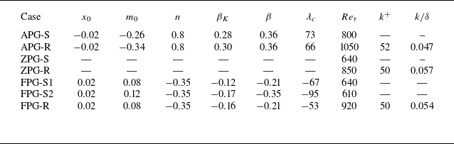


 Λc
 (1/F0)/(d(LF0)/dx)
 β
 βK

 f(y/δ)

 fu(y/δ)

 ruu(y/δ)

 ruv(y/δ)


 f(y/δ)
 fu(y/δ)

 rg

 T/Te
 u/Ue


 Trms′Prt/Tτ
 Trms′Prt/T0

 βK
 x/δ0=0
 x/δ0<0
 x/δ0>0


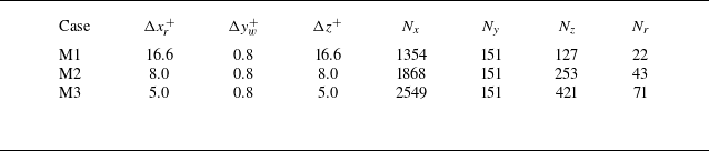
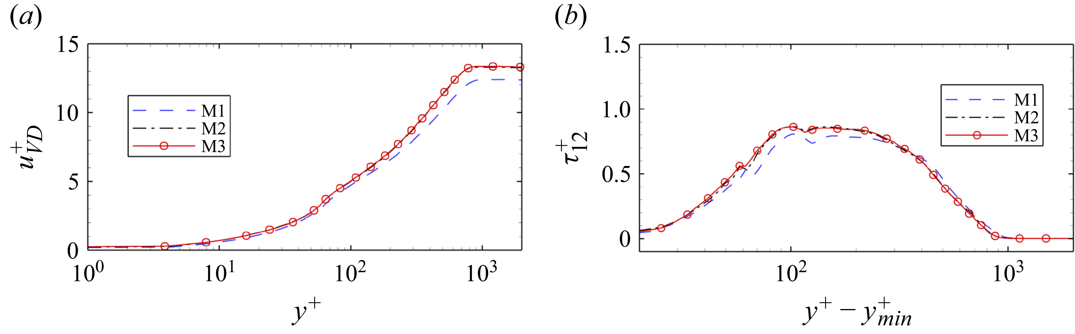
 uVD+
 τ12+
 τw

 τuu/(τw/(dL/dx))
 τvv/(τw/(dL/dx))

 βK
 up/u∞
 n


