2 Formulation of the problem

Steady-state MHD flows are governed by the following equations:

(2.1)$$\begin{eqnarray}\unicode[STIX]{x1D70C}(\boldsymbol{v}\boldsymbol{\cdot }\unicode[STIX]{x1D735})\boldsymbol{v}=-\unicode[STIX]{x1D735}p+\boldsymbol{J}\wedge \boldsymbol{B}-\unicode[STIX]{x1D70C}\unicode[STIX]{x1D735}\unicode[STIX]{x1D6F7},\end{eqnarray}$$

(2.2a,b)$$\begin{eqnarray}\unicode[STIX]{x1D735}\boldsymbol{\cdot }\boldsymbol{v}=0,\quad \boldsymbol{v}\boldsymbol{\cdot }\unicode[STIX]{x1D735}\unicode[STIX]{x1D70C}=0,\end{eqnarray}$$

(2.3)$$\begin{eqnarray}\displaystyle & \unicode[STIX]{x1D735}\wedge \boldsymbol{B}=\unicode[STIX]{x1D707}\boldsymbol{J}, & \displaystyle\end{eqnarray}$$

(2.4)$$\begin{eqnarray}\displaystyle & \unicode[STIX]{x1D735}\boldsymbol{\cdot }\boldsymbol{B}=0, & \displaystyle\end{eqnarray}$$

(2.5)$$\begin{eqnarray}\displaystyle & \boldsymbol{v}\wedge \boldsymbol{B}=0. & \displaystyle\end{eqnarray}$$

The symbols $\unicode[STIX]{x1D70C}$, $p$, $\boldsymbol{v}$, $\boldsymbol{B}$, $\boldsymbol{J}$, $\unicode[STIX]{x1D6F7}$ and $\unicode[STIX]{x1D707}$ denote density, pressure, velocity field, magnetic field (induction), electric current density, gravitational potential and the permeability constant, respectively. Here, we consider field-aligned flows in which the vectors $\boldsymbol{v}$ and $\boldsymbol{B}$ are parallel to each other and correlated by the following equation:

(2.6)$$\begin{eqnarray}\boldsymbol{B}=\unicode[STIX]{x1D6FC}(x,y,z)\boldsymbol{v},\end{eqnarray}$$

where $\unicode[STIX]{x1D6FC}(x,y,z)$ is an arbitrary function.

Using (2.2), (2.4) and (2.6), the magnetic field $\boldsymbol{B}$, velocity field $\boldsymbol{v}$ and the function $\unicode[STIX]{x1D6FC}(x,y,z)$ undergo the following equation:

(2.7a,b)$$\begin{eqnarray}\boldsymbol{v}\boldsymbol{\cdot }\unicode[STIX]{x1D735}\unicode[STIX]{x1D6FC}=0,\quad \boldsymbol{B}\boldsymbol{\cdot }\unicode[STIX]{x1D735}\unicode[STIX]{x1D6FC}=0.\end{eqnarray}$$

In Moawad & Ibrahim (Reference Moawad and Ibrahim2016) it was shown that the magnetic surfaces are defined by the relation $\unicode[STIX]{x1D6FC}(x,y,z)=\text{const}$.

Using (2.3) and (2.7) and the identity $(\boldsymbol{v}\boldsymbol{\cdot }\unicode[STIX]{x1D735})\boldsymbol{v}=\unicode[STIX]{x1D735}(v^{2}/2)-\boldsymbol{v}\wedge (\unicode[STIX]{x1D735}\wedge \boldsymbol{v})$, the momentum equation (2.1) changes to

(2.8)$$\begin{eqnarray}\left(\unicode[STIX]{x1D70C}-\frac{\unicode[STIX]{x1D6FC}^{2}}{\unicode[STIX]{x1D707}}\right)\unicode[STIX]{x1D74E}\wedge \boldsymbol{v}-\frac{1}{2}v^{2}\unicode[STIX]{x1D735}\left(\unicode[STIX]{x1D70C}-\frac{\unicode[STIX]{x1D6FC}^{2}}{\unicode[STIX]{x1D707}}\right)+\unicode[STIX]{x1D735}\left(p+\frac{1}{2}\unicode[STIX]{x1D70C}v^{2}\right)+\unicode[STIX]{x1D70C}\unicode[STIX]{x1D735}\unicode[STIX]{x1D6F7}=0,\end{eqnarray}$$

where $\unicode[STIX]{x1D74E}=\unicode[STIX]{x1D735}\wedge \boldsymbol{v}$ is the vorticity field.

Taking the scalar product of (2.8) by $\boldsymbol{v}$ and using (2.2) and (2.7) yield

(2.9)$$\begin{eqnarray}\boldsymbol{v}\boldsymbol{\cdot }\unicode[STIX]{x1D735}\left(p+{\textstyle \frac{1}{2}}\unicode[STIX]{x1D70C}v^{2}+\unicode[STIX]{x1D70C}\unicode[STIX]{x1D6F7}\right)=0.\end{eqnarray}$$

From the above formulations we find that field-aligned gravitating ideal MHD incompressible flows in three dimensions are governed by (2.2), (2.6)–(2.9).

3 First approach

3.1 Alfvénic flows

It is known that the Alfvén velocity is defined by

(3.1)$$\begin{eqnarray}\boldsymbol{v}_{A}\equiv \frac{\boldsymbol{B}}{\sqrt{\unicode[STIX]{x1D707}\unicode[STIX]{x1D70C}}}=\frac{\unicode[STIX]{x1D6FC}\boldsymbol{v}}{\sqrt{\unicode[STIX]{x1D707}\unicode[STIX]{x1D70C}}}.\end{eqnarray}$$

Therefore, Alfvénic flows ($\boldsymbol{v}=\boldsymbol{v}_{A}$) are those where $\unicode[STIX]{x1D70C}=\unicode[STIX]{x1D6FC}^{2}/\unicode[STIX]{x1D707}$. In this case (2.8) is reduced to

(3.2)$$\begin{eqnarray}\unicode[STIX]{x1D735}\left(p+{\textstyle \frac{1}{2}}\unicode[STIX]{x1D70C}v^{2}\right)+\unicode[STIX]{x1D70C}\unicode[STIX]{x1D735}\unicode[STIX]{x1D6F7}=0.\end{eqnarray}$$

3.1.1 Alfvénic flows where $\unicode[STIX]{x1D70C}$ and $\unicode[STIX]{x1D6FC}$ are constants

Theorem 1. The general three-dimensional solutions of the steady-state equations of Alfvénic, homogeneous, incompressible, field-aligned ($\boldsymbol{B}=\unicode[STIX]{x1D6FC}\boldsymbol{v}$, $\unicode[STIX]{x1D6FC}=\text{const}.$), ideal MHD flows in a gravitational field are given by,

(3.3)$$\begin{eqnarray}\left.\begin{array}{@{}c@{}}\boldsymbol{v}=\unicode[STIX]{x1D735}\wedge \boldsymbol{A},\\ p=k_{0}-{\textstyle \frac{1}{2}}\unicode[STIX]{x1D70C}v^{2}-\unicode[STIX]{x1D70C}\unicode[STIX]{x1D6F7},\\ \unicode[STIX]{x1D6F7}=\unicode[STIX]{x1D6F7}(x,y,z),\end{array}\right\}\end{eqnarray}$$

where $k_{0}$ is a real constant, $\boldsymbol{A}$ is an arbitrary three-dimensional vector quantity and $\unicode[STIX]{x1D6F7}(x,y,z)$ is an arbitrary three-dimensional scalar function.

Proof. Since the flow is homogeneous with $\unicode[STIX]{x1D6FC}=\text{const}.$, then $\boldsymbol{v}\boldsymbol{\cdot }\unicode[STIX]{x1D735}\unicode[STIX]{x1D70C}=\boldsymbol{v}\boldsymbol{\cdot }\unicode[STIX]{x1D735}\unicode[STIX]{x1D6FC}=0$. The incompressibility condition holds from $\unicode[STIX]{x1D735}\boldsymbol{\cdot }\boldsymbol{v}=\unicode[STIX]{x1D735}\boldsymbol{\cdot }(\unicode[STIX]{x1D735}\wedge \boldsymbol{A})=0$. Using the Alfvénic flow condition and substituting the pressure from (3.3) into (3.2), the momentum equation holds.

Remark.

If the fluid density is constant and $\unicode[STIX]{x1D6FC}$ is variable, the flow has the same solutions given in Theorem 1 and $\unicode[STIX]{x1D6FC}$ is obtained by solving the equation $\boldsymbol{v}\boldsymbol{\cdot }\unicode[STIX]{x1D735}\unicode[STIX]{x1D6FC}=0$.

3.1.2 Alfvénic flows where $\unicode[STIX]{x1D70C}$ and $\unicode[STIX]{x1D6FC}$ are variable functions that depend on $(x,y,z)$

Theorem 2. The general three-dimensional solutions of the steady-state equations of Alfvénic, inhomogeneous, incompressible, field-aligned ($\boldsymbol{B}=\unicode[STIX]{x1D6FC}\boldsymbol{v}$, $\unicode[STIX]{x1D6FC}\equiv \unicode[STIX]{x1D6FC}(x,y,z)$), ideal MHD flows in a gravitational field are given by,

(3.4)$$\begin{eqnarray}\left.\begin{array}{@{}c@{}}\boldsymbol{v}=\unicode[STIX]{x1D735}\wedge \boldsymbol{A},\\ \displaystyle p=-\int \unicode[STIX]{x1D70C}\unicode[STIX]{x1D6F7}^{\prime }(\unicode[STIX]{x1D70C})\,\text{d}\unicode[STIX]{x1D70C}-{\textstyle \frac{1}{2}}\unicode[STIX]{x1D70C}v^{2},\\ \unicode[STIX]{x1D6F7}\equiv \unicode[STIX]{x1D6F7}(\unicode[STIX]{x1D70C}),\quad \unicode[STIX]{x1D6FC}\equiv \unicode[STIX]{x1D6FC}(\unicode[STIX]{x1D70C}),\\ \boldsymbol{v}\boldsymbol{\cdot }\unicode[STIX]{x1D735}\unicode[STIX]{x1D70C}=0,\end{array}\right\}\end{eqnarray}$$

where the functions $\unicode[STIX]{x1D6F7}(\unicode[STIX]{x1D70C})$ and $\unicode[STIX]{x1D6FC}(\unicode[STIX]{x1D70C})$ are arbitrary functions of the fluid density. The density of the fluid can be determined using the characteristic equation of the last part of (3.4) as follows:

(3.5)$$\begin{eqnarray}\frac{\text{d}x}{{\displaystyle \frac{\unicode[STIX]{x2202}A_{z}}{\unicode[STIX]{x2202}y}}-{\displaystyle \frac{\unicode[STIX]{x2202}A_{y}}{\unicode[STIX]{x2202}z}}}=\frac{\text{d}y}{{\displaystyle \frac{\unicode[STIX]{x2202}A_{x}}{\unicode[STIX]{x2202}z}}-{\displaystyle \frac{\unicode[STIX]{x2202}A_{z}}{\unicode[STIX]{x2202}x}}}=\frac{\text{d}z}{{\displaystyle \frac{\unicode[STIX]{x2202}A_{y}}{\unicode[STIX]{x2202}x}}-{\displaystyle \frac{\unicode[STIX]{x2202}A_{x}}{\unicode[STIX]{x2202}y}}}=\frac{\text{d}\unicode[STIX]{x1D70C}}{0}.\end{eqnarray}$$

The integration of (3.5) yields

(3.6a-c)$$\begin{eqnarray}\unicode[STIX]{x1D713}_{1}(x,y,z)=\text{const}.,\quad \unicode[STIX]{x1D713}_{2}(x,y,z)=\text{const}.,\quad \unicode[STIX]{x1D70C}\equiv \unicode[STIX]{x1D70C}(\unicode[STIX]{x1D713}_{1},\unicode[STIX]{x1D713}_{2}),\end{eqnarray}$$

where $\unicode[STIX]{x1D70C}(\unicode[STIX]{x1D713}_{1},\unicode[STIX]{x1D713}_{2})$ is an arbitrary function of $\unicode[STIX]{x1D713}_{1}$ and $\unicode[STIX]{x1D713}_{2}$. The functions $\unicode[STIX]{x1D713}_{1}$ and $\unicode[STIX]{x1D713}_{2}$ are Euler potentials for the velocity field.

Proof. Since $\unicode[STIX]{x1D6FC}\equiv \unicode[STIX]{x1D6FC}(\unicode[STIX]{x1D70C})$, $\boldsymbol{v}\boldsymbol{\cdot }\unicode[STIX]{x1D735}\unicode[STIX]{x1D6FC}=\unicode[STIX]{x1D6FC}^{\prime }(\unicode[STIX]{x1D70C})\boldsymbol{v}\boldsymbol{\cdot }\unicode[STIX]{x1D735}\unicode[STIX]{x1D70C}=0$. The incompressibility condition holds from the first part of (3.4).

The scalar product of (3.2) and $\boldsymbol{v}$ leads to

(3.7)$$\begin{eqnarray}p+{\textstyle \frac{1}{2}}\unicode[STIX]{x1D70C}v^{2}+\unicode[STIX]{x1D70C}\unicode[STIX]{x1D6F7}=K(\unicode[STIX]{x1D70C}),\end{eqnarray}$$

where $K(\unicode[STIX]{x1D70C})$ is an arbitrary function of the fluid density.

By substituting (3.7) into (3.2) we get

(3.8)$$\begin{eqnarray}[K^{\prime }(\unicode[STIX]{x1D70C})-\unicode[STIX]{x1D6F7}]\unicode[STIX]{x1D735}\unicode[STIX]{x1D70C}=0.\end{eqnarray}$$

Hence, we obtain

(3.9a,b)$$\begin{eqnarray}\unicode[STIX]{x1D6F7}\equiv \unicode[STIX]{x1D6F7}(\unicode[STIX]{x1D70C})=K^{\prime }(\unicode[STIX]{x1D70C}),\quad p+{\textstyle \frac{1}{2}}\unicode[STIX]{x1D70C}v^{2}=p_{s}(\unicode[STIX]{x1D70C}),\end{eqnarray}$$

where $p_{s}(\unicode[STIX]{x1D70C})=K(\unicode[STIX]{x1D70C})-\unicode[STIX]{x1D70C}K^{\prime }(\unicode[STIX]{x1D70C})$ is a function of $\unicode[STIX]{x1D70C}$ that is determined in what follows.

From (3.2) and (3.9) we obtain

(3.10)$$\begin{eqnarray}[p_{s}^{\prime }(\unicode[STIX]{x1D70C})+\unicode[STIX]{x1D70C}\unicode[STIX]{x1D6F7}^{\prime }(\unicode[STIX]{x1D70C})]\unicode[STIX]{x1D735}\unicode[STIX]{x1D70C}=0.\end{eqnarray}$$

From (3.10), the function $p_{s}(\unicode[STIX]{x1D70C})$ is determined as,

(3.11)$$\begin{eqnarray}p_{s}=-\int \unicode[STIX]{x1D70C}\unicode[STIX]{x1D6F7}^{\prime }(\unicode[STIX]{x1D70C})\,\text{d}\unicode[STIX]{x1D70C}.\end{eqnarray}$$

Thus, equation (3.9) changes to

(3.12a,b)$$\begin{eqnarray}\unicode[STIX]{x1D6F7}\equiv \unicode[STIX]{x1D6F7}(\unicode[STIX]{x1D70C}),\quad p=-\int \unicode[STIX]{x1D70C}\unicode[STIX]{x1D6F7}^{\prime }(\unicode[STIX]{x1D70C})\,\text{d}\unicode[STIX]{x1D70C}-{\textstyle \frac{1}{2}}\unicode[STIX]{x1D70C}v^{2}.\end{eqnarray}$$

Substituting the pressure from (3.4) into (3.2), the momentum equation holds.

3.1.3 Examples

Example 3.1.1. Here, we consider some examples of Theorem 2. Let the vector potential of velocity be,

(3.13)$$\begin{eqnarray}\boldsymbol{A}=\left[X(x)+{\textstyle \frac{1}{2}}yz(y+z)\right]\boldsymbol{e}_{x}+\left[Y(y)+{\textstyle \frac{1}{2}}xz(x+z)\right]\boldsymbol{e}_{y}+\left[Z(z)+{\textstyle \frac{1}{2}}xy(x+y)\right]\boldsymbol{e}_{z},\end{eqnarray}$$

where $X(x)$, $Y(y)$, and $Z(z)$ are arbitrary functions. Therefore, the velocity vector can be determined as,

(3.14)$$\begin{eqnarray}\boldsymbol{v}=x(y-z)\boldsymbol{e}_{x}+y(z-x)\boldsymbol{e}_{y}+z(x-y)\boldsymbol{e}_{z}.\end{eqnarray}$$

Using (3.5) and (3.6), the density can be obtained as an arbitrary function of the functions $x+y+z$ and $xyz$,

(3.15)$$\begin{eqnarray}\unicode[STIX]{x1D70C}=\unicode[STIX]{x1D70C}(x+y+z,xyz).\end{eqnarray}$$

For this example and the next two examples, the gravitational potential $\unicode[STIX]{x1D6F7}$ and the function $\unicode[STIX]{x1D6FC}$ are arbitrary functions of $\unicode[STIX]{x1D70C}$. The gas pressure can be obtained using the second part of (3.10).

Example 3.1.2. Let the vector potential of velocity be,

(3.16)$$\begin{eqnarray}\boldsymbol{A}=\left[X(x)+{\textstyle \frac{1}{2}}(y^{2}+z^{2})\right]\boldsymbol{e}_{x}+\left[Y(y)+{\textstyle \frac{1}{2}}(x^{2}+z^{2})\right]\boldsymbol{e}_{y}+\left[Z(z)+{\textstyle \frac{1}{2}}(x^{2}+y^{2})\right]\boldsymbol{e}_{z},\end{eqnarray}$$

where $X(x)$, $Y(y)$ and $Z(z)$ are arbitrary functions. Therefore, the velocity vector can be determined as,

(3.17)$$\begin{eqnarray}\boldsymbol{v}=(y-z)\boldsymbol{e}_{x}+(z-x)\boldsymbol{e}_{y}+(x-y)\boldsymbol{e}_{z}.\end{eqnarray}$$

Using (3.5) and (3.6), the density can be obtained as an arbitrary function of the functions $x+y+z$ and $x^{2}+y^{2}+z^{2}$,

(3.18)$$\begin{eqnarray}\unicode[STIX]{x1D70C}=\unicode[STIX]{x1D70C}(x+y+z,x^{2}+y^{2}+z^{2}).\end{eqnarray}$$

Example 3.1.3. Let the vector potential of velocity be,

(3.19)$$\begin{eqnarray}\boldsymbol{A}=[X_{1}(x)+xyzX_{2}(x)]\boldsymbol{e}_{x}+Y(y)\boldsymbol{e}_{y}+[Z_{1}(z)+xyzZ_{2}(z)]\boldsymbol{e}_{z},\end{eqnarray}$$

where $X_{1}(x),X_{2}(x),Y(y),Z_{1}(z)$ and $Z_{2}(z)$ are arbitrary functions. Therefore, the velocity vector can be determined as,

(3.20)$$\begin{eqnarray}\boldsymbol{v}=xzZ_{2}(z)\boldsymbol{e}_{x}+y[xX_{2}(x)-zZ_{2}(z)]\boldsymbol{e}_{y}-xzX_{2}(x)\boldsymbol{e}_{z}.\end{eqnarray}$$

Using (3.5) and (3.6), the density can be obtained as an arbitrary function of the functions $xyz$ and $\int X_{2}(x)\,\text{d}x+\int Z_{2}(z)\,\text{d}z$:

(3.21)$$\begin{eqnarray}\unicode[STIX]{x1D70C}=\unicode[STIX]{x1D70C}(\unicode[STIX]{x1D713}_{1},\unicode[STIX]{x1D713}_{2}),\quad \text{with}~\unicode[STIX]{x1D713}_{1}=xyz~\text{and}~\unicode[STIX]{x1D713}_{2}=\int X_{2}(x)\,\text{d}x+\int Z_{2}(z)\,\text{d}z.\end{eqnarray}$$

The above examples show the variety of three-dimensional solutions to the physical variables $\unicode[STIX]{x1D70C},\unicode[STIX]{x1D6FC},p,\unicode[STIX]{x1D6F7},\boldsymbol{v}$ and $\boldsymbol{B}$ that can be obtained for field-aligned incompressible MHD flows in the presence of a gravitational field.

3.2 Non-Alfvénic flows

In this subsection we consider the general field-aligned incompressible MHD flow.

Theorem 3. Let $\boldsymbol{v}$ be any solution of Beltrami incompressible flow. The steady-state equations of non-Alfvénic, inhomogeneous, incompressible, field-aligned ($\boldsymbol{B}=\unicode[STIX]{x1D6FC}\boldsymbol{v}$, $\unicode[STIX]{x1D6FC}\equiv \unicode[STIX]{x1D6FC}(x,y,z)$), ideal MHD flows in a gravitational field have the following set of three-dimensional solutions:

(3.22)$$\begin{eqnarray}\left.\begin{array}{@{}c@{}}\displaystyle p=K(\unicode[STIX]{x1D70C})-\unicode[STIX]{x1D70C}\left[K^{\prime }(\unicode[STIX]{x1D70C})+\frac{v^{2}\unicode[STIX]{x1D6FC}\unicode[STIX]{x1D6FC}^{\prime }}{\unicode[STIX]{x1D707}}\right],\\ \displaystyle \unicode[STIX]{x1D6F7}=K^{\prime }(\unicode[STIX]{x1D70C})-\frac{1}{2}v^{2}\left(\unicode[STIX]{x1D70C}-\frac{\unicode[STIX]{x1D6FC}^{2}}{\unicode[STIX]{x1D707}}\right)^{\prime },\\ \unicode[STIX]{x1D6FC}\equiv \unicode[STIX]{x1D6FC}(\unicode[STIX]{x1D70C}),\end{array}\right\}\end{eqnarray}$$

where $\unicode[STIX]{x1D714}=\unicode[STIX]{x1D735}\wedge \boldsymbol{v}$ is the vorticity field and $\unicode[STIX]{x1D6FD}(x,y,z)$ is an arbitrary function of space. The functions $\unicode[STIX]{x1D6FC}(\unicode[STIX]{x1D70C})$ and $K(\unicode[STIX]{x1D70C})$ are arbitrary functions of the fluid density.

Proof. To satisfy (2.9), we consider the quantity $p+\frac{1}{2}\unicode[STIX]{x1D70C}v^{2}+\unicode[STIX]{x1D70C}\unicode[STIX]{x1D6F7}$ as an arbitrary function of the density $\unicode[STIX]{x1D70C}$, i.e. $p+\frac{1}{2}\unicode[STIX]{x1D70C}v^{2}+\unicode[STIX]{x1D70C}\unicode[STIX]{x1D6F7}=K(\unicode[STIX]{x1D70C})$.

The incompressible Beltrami flows are governed by the equations,

(3.23a,b)$$\begin{eqnarray}\unicode[STIX]{x1D735}\wedge \boldsymbol{v}=\unicode[STIX]{x1D706}\boldsymbol{v},\quad \unicode[STIX]{x1D735}\boldsymbol{\cdot }\boldsymbol{v}=0,\end{eqnarray}$$

where $\unicode[STIX]{x1D706}$ is a function of $\unicode[STIX]{x1D70C}$. Therefore, equation (2.8) changes to

(3.24)$$\begin{eqnarray}-\frac{1}{2}v^{2}\unicode[STIX]{x1D735}\left(\unicode[STIX]{x1D70C}-\frac{\unicode[STIX]{x1D6FC}^{2}}{\unicode[STIX]{x1D707}}\right)+[K^{\prime }(\unicode[STIX]{x1D70C})-\unicode[STIX]{x1D6F7}]\unicode[STIX]{x1D735}\unicode[STIX]{x1D70C}=0.\end{eqnarray}$$

The cross-product of (3.24) and $\unicode[STIX]{x1D735}\unicode[STIX]{x1D70C}$ yields

(3.25a,b)$$\begin{eqnarray}\unicode[STIX]{x1D6FC}=\unicode[STIX]{x1D6FC}(\unicode[STIX]{x1D70C}),\quad \unicode[STIX]{x1D6F7}=K^{\prime }(\unicode[STIX]{x1D70C})-\frac{1}{2}v^{2}\left(\unicode[STIX]{x1D70C}-\frac{\unicode[STIX]{x1D6FC}^{2}}{\unicode[STIX]{x1D707}}\right)^{\prime }.\end{eqnarray}$$

Therefore, the pressure is obtained as,

(3.26)$$\begin{eqnarray}p=K(\unicode[STIX]{x1D70C})-\frac{1}{2}\unicode[STIX]{x1D70C}v^{2}-\unicode[STIX]{x1D70C}\unicode[STIX]{x1D6F7}=K(\unicode[STIX]{x1D70C})-\unicode[STIX]{x1D70C}\left[K^{\prime }(\unicode[STIX]{x1D70C})+\frac{v^{2}\unicode[STIX]{x1D6FC}\unicode[STIX]{x1D6FC}^{\prime }}{\unicode[STIX]{x1D707}}\right],\end{eqnarray}$$

which implies the momentum equation holds true.

Example 3.1.4 (Arnold–Beltrami–Childress (ABC) flow).

For constant $\unicode[STIX]{x1D706}$, equation (3.23) obeys the following ABC flow (Dombre et al. Reference Dombre, Frisch, Greene, Hénon, Mehr and Soward1986; Ershkov Reference Ershkov2016):

(3.27)$$\begin{eqnarray}\displaystyle \boldsymbol{v}=[C\cos (\unicode[STIX]{x1D706}y)+A\sin (\unicode[STIX]{x1D706}z)]\boldsymbol{e}_{x}+[A\cos (\unicode[STIX]{x1D706}z)+B\sin (\unicode[STIX]{x1D706}x)]\boldsymbol{e}_{y}+[B\cos (\unicode[STIX]{x1D706}x)+C\sin (\unicode[STIX]{x1D706}y)]\boldsymbol{e}_{z}. & & \displaystyle \nonumber\\ \displaystyle & & \displaystyle\end{eqnarray}$$

Using (3.22), we obtain each of the pressures, the gravitational potential and the proportional factor $\unicode[STIX]{x1D6FC}$. Fluid density can be determined by solving the equation $\boldsymbol{v}\boldsymbol{\cdot }\unicode[STIX]{x1D735}\unicode[STIX]{x1D70C}=0$. For example, it can be taken as an arbitrary function of $C\sin (\unicode[STIX]{x1D706}y)+B\cos (\unicode[STIX]{x1D706}x)$.

For some recent results on Beltrami flows, see Enciso & Peralta-Salas (Reference Enciso and Peralta-Salas2012, Reference Enciso and Peralta-Salas2015), Enciso, Poyato & Soler (Reference Enciso, Poyato and Soler2016) and Enciso & Peralta-Salas (Reference Enciso and Peralta-Salas2016) and references therein. In Enciso & Peralta-Salas (Reference Enciso and Peralta-Salas2012, Reference Enciso and Peralta-Salas2015), Beltrami fields for non-zero constant were constructed. In Enciso et al. (Reference Enciso, Poyato and Soler2016), the existence of Beltrami fields with a non-constant proportionality factor $\unicode[STIX]{x1D706}$ was considered. They showed that there are no non-trivial Beltrami fields whenever $\unicode[STIX]{x1D706}$ is variable. By reformulating this problem as a constrained evolution equation on a surface, they found an explicit differential equation that $\unicode[STIX]{x1D706}$ must satisfy whenever there is a non-trivial Beltrami field with this factor. Beltrami flows are also called force-free magnetic fields in MHD, since the term $(\unicode[STIX]{x1D735}\wedge \boldsymbol{v})\wedge \boldsymbol{v}$ models the Lorentz force when $\boldsymbol{v}$ represents the magnetic field, see Moawad (Reference Moawad2014) and references therein. By establishing an elementary identity, uniqueness results for Beltrami flow in both bounded and unbounded domains with a non-empty boundary were obtained by Zeng & Zhang (Reference Zeng and Zhang2018). They used that identity to deal with Maxwell and Stokes eigenvalue problems. An early remarkable application of force-free solutions for astrophysical magnetic fields was achieved by Chandrasekhar & Kendall (Reference Chandrasekhar and Kendall1957).

Theorem 4. The steady-state equations of non-Alfvénic, inhomogeneous, incompressible, field-aligned ($\boldsymbol{B}=\unicode[STIX]{x1D6FC}\boldsymbol{v}$, $\unicode[STIX]{x1D6FC}\equiv \unicode[STIX]{x1D6FC}(x,y,z)$), ideal MHD flows in a gravitational field have the following set of general three-dimensional solutions:

(3.28)$$\begin{eqnarray}\left.\begin{array}{@{}c@{}}\boldsymbol{v}=f(\unicode[STIX]{x1D6FC},\unicode[STIX]{x1D70C})\unicode[STIX]{x1D735}\unicode[STIX]{x1D6FC}\wedge \unicode[STIX]{x1D735}\unicode[STIX]{x1D70C},\\ p=K(\unicode[STIX]{x1D70C})-{\textstyle \frac{1}{2}}\unicode[STIX]{x1D70C}v^{2}+\unicode[STIX]{x1D70C}\unicode[STIX]{x1D6F7},\\ \unicode[STIX]{x1D6F7}=K^{\prime }(\unicode[STIX]{x1D70C})-f\unicode[STIX]{x1D74E}\boldsymbol{\cdot }\unicode[STIX]{x1D735}\unicode[STIX]{x1D736}-{\textstyle \frac{1}{2}}v^{2},\end{array}\right\}\end{eqnarray}$$

with the compatibility condition,

(3.29)$$\begin{eqnarray}\frac{\unicode[STIX]{x1D735}\unicode[STIX]{x1D70C}\boldsymbol{\cdot }\unicode[STIX]{x1D735}\wedge (\unicode[STIX]{x1D735}\unicode[STIX]{x1D6FC}\wedge \unicode[STIX]{x1D735}\unicode[STIX]{x1D70C})}{\Vert \unicode[STIX]{x1D735}\unicode[STIX]{x1D6FC}\wedge \unicode[STIX]{x1D735}\unicode[STIX]{x1D70C}\Vert ^{2}}=\frac{1}{f}\frac{\unicode[STIX]{x2202}f}{\unicode[STIX]{x2202}\unicode[STIX]{x1D6FC}}-\frac{\unicode[STIX]{x1D6FC}}{\unicode[STIX]{x1D707}\unicode[STIX]{x1D70C}-\unicode[STIX]{x1D6FC}^{2}}\equiv \unicode[STIX]{x1D712}(\unicode[STIX]{x1D6FC},\unicode[STIX]{x1D70C}).\end{eqnarray}$$

Proof. The equations $\boldsymbol{v}\boldsymbol{\cdot }\unicode[STIX]{x1D735}\unicode[STIX]{x1D6FC}=0$ and $\boldsymbol{v}\boldsymbol{\cdot }\unicode[STIX]{x1D735}\unicode[STIX]{x1D70C}=0$ are clearly satisfied.

Using the vector identity $\unicode[STIX]{x1D735}\boldsymbol{\cdot }(\boldsymbol{A}\wedge \boldsymbol{B})=\boldsymbol{B}\boldsymbol{\cdot }\unicode[STIX]{x1D735}\wedge \boldsymbol{A}-\boldsymbol{A}\boldsymbol{\cdot }\unicode[STIX]{x1D735}\wedge \boldsymbol{B}$, we have,

(3.30)$$\begin{eqnarray}\displaystyle \unicode[STIX]{x1D735}\boldsymbol{\cdot }\boldsymbol{v} & = & \displaystyle f\unicode[STIX]{x1D735}\boldsymbol{\cdot }(\unicode[STIX]{x1D735}\unicode[STIX]{x1D6FC}\wedge \unicode[STIX]{x1D735}\unicode[STIX]{x1D70C})+\unicode[STIX]{x1D735}f\boldsymbol{\cdot }(\unicode[STIX]{x1D735}\unicode[STIX]{x1D6FC}\wedge \unicode[STIX]{x1D735}\unicode[STIX]{x1D70C})\nonumber\\ \displaystyle & = & \displaystyle f\unicode[STIX]{x1D735}\boldsymbol{\cdot }(\unicode[STIX]{x1D735}\unicode[STIX]{x1D6FC}\wedge \unicode[STIX]{x1D735}\unicode[STIX]{x1D70C})+\left(\frac{\unicode[STIX]{x2202}f}{\unicode[STIX]{x2202}\unicode[STIX]{x1D6FC}}\unicode[STIX]{x1D735}\unicode[STIX]{x1D6FC}+\frac{\unicode[STIX]{x2202}f}{\unicode[STIX]{x2202}\unicode[STIX]{x1D70C}}\unicode[STIX]{x1D735}\unicode[STIX]{x1D70C}\right)\boldsymbol{\cdot }(\unicode[STIX]{x1D735}\unicode[STIX]{x1D6FC}\wedge \unicode[STIX]{x1D735}\unicode[STIX]{x1D70C})=0.\end{eqnarray}$$

Thus, the incompressibility condition holds true. To show that the momentum equation is achieved, we use the relation $p+\frac{1}{2}\unicode[STIX]{x1D70C}v^{2}+\unicode[STIX]{x1D70C}\unicode[STIX]{x1D6F7}=K(\unicode[STIX]{x1D70C})$ into (2.8) which changes to

(3.31)$$\begin{eqnarray}\left(\unicode[STIX]{x1D70C}-\frac{\unicode[STIX]{x1D6FC}^{2}}{\unicode[STIX]{x1D707}}\right)\unicode[STIX]{x1D74E}\wedge \boldsymbol{v}-\frac{1}{2}v^{2}\unicode[STIX]{x1D735}\left(\unicode[STIX]{x1D70C}-\frac{\unicode[STIX]{x1D6FC}^{2}}{\unicode[STIX]{x1D707}}\right)+[K^{\prime }(\unicode[STIX]{x1D70C})-\unicode[STIX]{x1D6F7}]\unicode[STIX]{x1D735}\unicode[STIX]{x1D70C}=0.\end{eqnarray}$$

The cross-product of (3.31) and $\unicode[STIX]{x1D735}\unicode[STIX]{x1D70C}$ yields

(3.32)$$\begin{eqnarray}\left[\left(\unicode[STIX]{x1D70C}-\frac{\unicode[STIX]{x1D6FC}^{2}}{\unicode[STIX]{x1D707}}\right)(\unicode[STIX]{x1D74E}\boldsymbol{\cdot }\unicode[STIX]{x1D735}\unicode[STIX]{x1D70C})f+\frac{\unicode[STIX]{x1D6FC}v^{2}}{\unicode[STIX]{x1D707}}\right]\unicode[STIX]{x1D735}\unicode[STIX]{x1D6FC}\wedge \unicode[STIX]{x1D735}\unicode[STIX]{x1D70C}=0,\end{eqnarray}$$

which implies

(3.33)$$\begin{eqnarray}\unicode[STIX]{x1D74E}\boldsymbol{\cdot }\unicode[STIX]{x1D735}\unicode[STIX]{x1D70C}=-\frac{\unicode[STIX]{x1D6FC}v^{2}}{f(\unicode[STIX]{x1D707}\unicode[STIX]{x1D70C}-\unicode[STIX]{x1D6FC}^{2})}.\end{eqnarray}$$

Substituting $\boldsymbol{v}=f(\unicode[STIX]{x1D6FC},\unicode[STIX]{x1D70C})\unicode[STIX]{x1D735}\unicode[STIX]{x1D6FC}\wedge \unicode[STIX]{x1D735}\unicode[STIX]{x1D70C}$ in (3.31) and using the vector identity

(3.34)$$\begin{eqnarray}\unicode[STIX]{x1D74E}\wedge \boldsymbol{v}=f\unicode[STIX]{x1D74E}\wedge (\unicode[STIX]{x1D735}\unicode[STIX]{x1D6FC}\wedge \unicode[STIX]{x1D735}\unicode[STIX]{x1D70C})=f[(\unicode[STIX]{x1D74E}\boldsymbol{\cdot }\unicode[STIX]{x1D735}\unicode[STIX]{x1D70C})\unicode[STIX]{x1D735}\unicode[STIX]{x1D6FC}-(\unicode[STIX]{x1D74E}\boldsymbol{\cdot }\unicode[STIX]{x1D735}\unicode[STIX]{x1D6FC})\unicode[STIX]{x1D735}\unicode[STIX]{x1D70C}],\end{eqnarray}$$

we get

(3.35)$$\begin{eqnarray}\left[\left(\unicode[STIX]{x1D70C}-\frac{\unicode[STIX]{x1D6FC}^{2}}{\unicode[STIX]{x1D707}}\right)f(\unicode[STIX]{x1D74E}\boldsymbol{\cdot }\unicode[STIX]{x1D735}\unicode[STIX]{x1D70C})+\frac{\unicode[STIX]{x1D6FC}v^{2}}{\unicode[STIX]{x1D707}}\right]\unicode[STIX]{x1D735}\unicode[STIX]{x1D6FC}+\left(K^{\prime }(\unicode[STIX]{x1D70C})-\unicode[STIX]{x1D6F7}-f\unicode[STIX]{x1D74E}\boldsymbol{\cdot }\unicode[STIX]{x1D735}\unicode[STIX]{x1D6FC}-\frac{1}{2}v^{2}\right)\unicode[STIX]{x1D735}\unicode[STIX]{x1D70C}=0.\end{eqnarray}$$

The quantity multiplied by $\unicode[STIX]{x1D735}\unicode[STIX]{x1D6FC}$ equals zero from (3.33), hence we get

(3.36)$$\begin{eqnarray}\unicode[STIX]{x1D6F7}=K^{\prime }(\unicode[STIX]{x1D70C})-f\unicode[STIX]{x1D74E}\boldsymbol{\cdot }\unicode[STIX]{x1D735}\unicode[STIX]{x1D6FC}-{\textstyle \frac{1}{2}}v^{2}.\end{eqnarray}$$

What remains is the proof of the compatibility conditions in (3.29) which we show in what follows.

(3.37)$$\begin{eqnarray}\displaystyle \unicode[STIX]{x1D74E} & = & \displaystyle \unicode[STIX]{x1D735}\wedge \boldsymbol{v}=\unicode[STIX]{x1D735}\wedge (f\unicode[STIX]{x1D735}\unicode[STIX]{x1D6FC}\wedge \unicode[STIX]{x1D735}\unicode[STIX]{x1D70C})\nonumber\\ \displaystyle & = & \displaystyle f\unicode[STIX]{x1D735}\wedge (\unicode[STIX]{x1D735}\unicode[STIX]{x1D6FC}\wedge \unicode[STIX]{x1D735}\unicode[STIX]{x1D70C})+\unicode[STIX]{x1D735}f\wedge (\unicode[STIX]{x1D735}\unicode[STIX]{x1D6FC}\wedge \unicode[STIX]{x1D735}\unicode[STIX]{x1D70C})\nonumber\\ \displaystyle & = & \displaystyle f\unicode[STIX]{x1D735}\wedge (\unicode[STIX]{x1D735}\unicode[STIX]{x1D6FC}\wedge \unicode[STIX]{x1D735}\unicode[STIX]{x1D70C})+(\unicode[STIX]{x1D735}f\boldsymbol{\cdot }\unicode[STIX]{x1D735}\unicode[STIX]{x1D70C})\unicode[STIX]{x1D735}\unicode[STIX]{x1D6FC}-(\unicode[STIX]{x1D735}f\boldsymbol{\cdot }\unicode[STIX]{x1D735}\unicode[STIX]{x1D6FC})\unicode[STIX]{x1D735}\unicode[STIX]{x1D70C}.\end{eqnarray}$$

Since $f=f(\unicode[STIX]{x1D6FC},\unicode[STIX]{x1D70C})$,

(3.38)$$\begin{eqnarray}\displaystyle \unicode[STIX]{x1D735}f\boldsymbol{\cdot }\unicode[STIX]{x1D735}\unicode[STIX]{x1D70C} & = & \displaystyle \left(\frac{\unicode[STIX]{x2202}f}{\unicode[STIX]{x2202}\unicode[STIX]{x1D6FC}}\unicode[STIX]{x1D735}\unicode[STIX]{x1D6FC}+\frac{\unicode[STIX]{x2202}f}{\unicode[STIX]{x2202}\unicode[STIX]{x1D70C}}\unicode[STIX]{x1D735}\unicode[STIX]{x1D70C}\right)\boldsymbol{\cdot }\unicode[STIX]{x1D735}\unicode[STIX]{x1D70C}\nonumber\\ \displaystyle & = & \displaystyle \frac{\unicode[STIX]{x2202}f}{\unicode[STIX]{x2202}\unicode[STIX]{x1D6FC}}\unicode[STIX]{x1D735}\unicode[STIX]{x1D6FC}\boldsymbol{\cdot }\unicode[STIX]{x1D735}\unicode[STIX]{x1D70C}+\frac{\unicode[STIX]{x2202}f}{\unicode[STIX]{x2202}\unicode[STIX]{x1D70C}}\Vert \unicode[STIX]{x1D735}\unicode[STIX]{x1D70C}\Vert ^{2},\end{eqnarray}$$

(3.39)$$\begin{eqnarray}\displaystyle \unicode[STIX]{x1D735}f\boldsymbol{\cdot }\unicode[STIX]{x1D735}\unicode[STIX]{x1D6FC} & = & \displaystyle \left(\frac{\unicode[STIX]{x2202}f}{\unicode[STIX]{x2202}\unicode[STIX]{x1D6FC}}\unicode[STIX]{x1D735}\unicode[STIX]{x1D6FC}+\frac{\unicode[STIX]{x2202}f}{\unicode[STIX]{x2202}\unicode[STIX]{x1D70C}}\unicode[STIX]{x1D735}\unicode[STIX]{x1D70C}\right)\boldsymbol{\cdot }\unicode[STIX]{x1D735}\unicode[STIX]{x1D6FC}\nonumber\\ \displaystyle & = & \displaystyle \frac{\unicode[STIX]{x2202}f}{\unicode[STIX]{x2202}\unicode[STIX]{x1D6FC}}\Vert \unicode[STIX]{x1D735}\unicode[STIX]{x1D6FC}\Vert ^{2}+\frac{\unicode[STIX]{x2202}f}{\unicode[STIX]{x2202}\unicode[STIX]{x1D70C}}\unicode[STIX]{x1D735}\unicode[STIX]{x1D70C}\boldsymbol{\cdot }\unicode[STIX]{x1D735}\unicode[STIX]{x1D6FC}.\end{eqnarray}$$

Therefore (3.37) changes to

(3.40)$$\begin{eqnarray}\displaystyle \unicode[STIX]{x1D74E} & = & \displaystyle f\unicode[STIX]{x1D735}\wedge (\unicode[STIX]{x1D735}\unicode[STIX]{x1D6FC}\wedge \unicode[STIX]{x1D735}\unicode[STIX]{x1D70C})+\left(\frac{\unicode[STIX]{x2202}f}{\unicode[STIX]{x2202}\unicode[STIX]{x1D6FC}}\unicode[STIX]{x1D735}\unicode[STIX]{x1D6FC}\boldsymbol{\cdot }\unicode[STIX]{x1D735}\unicode[STIX]{x1D70C}+\frac{\unicode[STIX]{x2202}f}{\unicode[STIX]{x2202}\unicode[STIX]{x1D70C}}\Vert \unicode[STIX]{x1D735}\unicode[STIX]{x1D70C}\Vert ^{2}\right)\unicode[STIX]{x1D735}\unicode[STIX]{x1D6FC}\nonumber\\ \displaystyle & & \displaystyle -\left(\frac{\unicode[STIX]{x2202}f}{\unicode[STIX]{x2202}\unicode[STIX]{x1D6FC}}\Vert \unicode[STIX]{x1D735}\unicode[STIX]{x1D6FC}\Vert ^{2}+\frac{\unicode[STIX]{x2202}f}{\unicode[STIX]{x2202}\unicode[STIX]{x1D70C}}\unicode[STIX]{x1D735}\unicode[STIX]{x1D70C}\boldsymbol{\cdot }\unicode[STIX]{x1D735}\unicode[STIX]{x1D6FC}\right)\unicode[STIX]{x1D735}\unicode[STIX]{x1D70C}.\end{eqnarray}$$

Taking the scalar product of (3.40) and $\unicode[STIX]{x1D735}\unicode[STIX]{x1D70C}$ we get

(3.41)$$\begin{eqnarray}\unicode[STIX]{x1D74E}\boldsymbol{\cdot }\unicode[STIX]{x1D735}\unicode[STIX]{x1D70C}=f\unicode[STIX]{x1D735}\unicode[STIX]{x1D70C}\boldsymbol{\cdot }\unicode[STIX]{x1D735}\wedge (\unicode[STIX]{x1D735}\unicode[STIX]{x1D6FC}\wedge \unicode[STIX]{x1D735}\unicode[STIX]{x1D70C})+\frac{\unicode[STIX]{x2202}f}{\unicode[STIX]{x2202}\unicode[STIX]{x1D6FC}}[(\unicode[STIX]{x1D735}\unicode[STIX]{x1D6FC}\boldsymbol{\cdot }\unicode[STIX]{x1D735}\unicode[STIX]{x1D70C})^{2}-\Vert \unicode[STIX]{x1D735}\unicode[STIX]{x1D6FC}\Vert ^{2}\Vert \unicode[STIX]{x1D735}\unicode[STIX]{x1D70C}\Vert ^{2}].\end{eqnarray}$$

Using the vector identity,

(3.42)$$\begin{eqnarray}\Vert \boldsymbol{A}\wedge \boldsymbol{B}\Vert ^{2}+(\boldsymbol{A}\boldsymbol{\cdot }\boldsymbol{B})^{2}=\Vert \boldsymbol{A}\Vert ^{2}\Vert \boldsymbol{B}\Vert ^{2},\end{eqnarray}$$

equation (3.41) changes to

(3.43)$$\begin{eqnarray}\unicode[STIX]{x1D74E}\boldsymbol{\cdot }\unicode[STIX]{x1D735}\unicode[STIX]{x1D70C}=f\unicode[STIX]{x1D735}\unicode[STIX]{x1D70C}\boldsymbol{\cdot }\unicode[STIX]{x1D735}\wedge (\unicode[STIX]{x1D735}\unicode[STIX]{x1D6FC}\wedge \unicode[STIX]{x1D735}\unicode[STIX]{x1D70C})+\frac{\unicode[STIX]{x2202}f}{\unicode[STIX]{x2202}\unicode[STIX]{x1D6FC}}\Vert \unicode[STIX]{x1D735}\unicode[STIX]{x1D6FC}\wedge \unicode[STIX]{x1D735}\unicode[STIX]{x1D70C}\Vert ^{2}.\end{eqnarray}$$

From (3.33) and (3.43), we obtain the compatibility condition shown in (3.29).

3.2.1 Examples

Example 3.2.1. Here, we consider some examples of Theorem 4. Consider the functions $\unicode[STIX]{x1D6FC}$ and $\unicode[STIX]{x1D70C}$ as,

(3.44)$$\begin{eqnarray}\displaystyle & \unicode[STIX]{x1D6FC}=a_{1}x+b_{1}y+c_{1}z+d_{1}, & \displaystyle\end{eqnarray}$$

(3.45)$$\begin{eqnarray}\displaystyle & \unicode[STIX]{x1D70C}=a_{2}x+b_{2}y+c_{2}z+d_{2}, & \displaystyle\end{eqnarray}$$

where $a_{i},b_{i},c_{i}$ and $d_{i}$, $(i=1,2)$ are real constants. The constant $d_{2}$ must be positive where one could in principle always add it to make the density positive (provided that the density remains bounded over the domain). Therefore, the velocity vector can be determined as,

(3.46)$$\begin{eqnarray}\boldsymbol{v}=f[(b_{1}c_{2}-c_{1}b_{2})\boldsymbol{e}_{x}+(c_{1}a_{2}-a_{1}c_{2})\boldsymbol{e}_{y}+(a_{1}b_{2}-b_{1}a_{2})\boldsymbol{e}_{z}].\end{eqnarray}$$

Using the compatibility condition (3.29), the function $f$ is obtained as,

(3.47)$$\begin{eqnarray}f=\frac{R}{\sqrt{\unicode[STIX]{x1D707}\unicode[STIX]{x1D70C}-\unicode[STIX]{x1D6FC}^{2}}},\end{eqnarray}$$

where $R\equiv R(\unicode[STIX]{x1D70C})$ is an arbitrary function of $\unicode[STIX]{x1D70C}$.

The gravitational potential is given by,

(3.48)$$\begin{eqnarray}\unicode[STIX]{x1D6F7}=K^{\prime }(\unicode[STIX]{x1D70C})-\frac{A^{2}R^{2}}{\unicode[STIX]{x1D707}\unicode[STIX]{x1D70C}-\unicode[STIX]{x1D6FC}^{2}}\left[\frac{R^{\prime }}{R}-\frac{\unicode[STIX]{x1D707}}{2(\unicode[STIX]{x1D707}\unicode[STIX]{x1D70C}-\unicode[STIX]{x1D6FC}^{2})}+\frac{1}{2}\right],\end{eqnarray}$$

where $A^{2}=(b_{1}c_{2}-c_{1}b_{2})^{2}+(c_{1}a_{2}-a_{1}c_{2})^{2}+(a_{1}b_{2}-b_{1}a_{2})^{2}$.

Example 3.2.2. Consider the functions $\unicode[STIX]{x1D6FC}$ and $\unicode[STIX]{x1D70C}$ as,

(3.49)$$\begin{eqnarray}\displaystyle & \unicode[STIX]{x1D6FC}=\unicode[STIX]{x1D711}(\unicode[STIX]{x1D709}_{1}),\quad \unicode[STIX]{x1D709}_{1}=a_{1}x+b_{1}y+c_{1}z+d_{1}, & \displaystyle\end{eqnarray}$$

(3.50)$$\begin{eqnarray}\displaystyle & \unicode[STIX]{x1D70C}=\unicode[STIX]{x1D713}(\unicode[STIX]{x1D709}_{2})+C,\quad \unicode[STIX]{x1D709}_{2}=a_{2}x+b_{2}y+c_{2}z+d_{2}, & \displaystyle\end{eqnarray}$$

where $\unicode[STIX]{x1D711}$ and $\unicode[STIX]{x1D713}$ are arbitrary functions, and $a_{i},b_{i},c_{i}$ and $d_{i}$, $(i=1,2)$ are real constants with $C$ a positive constant always added to make the density positive and bounded over the domain.

Therefore

(3.51a,b)$$\begin{eqnarray}\unicode[STIX]{x1D735}\unicode[STIX]{x1D6FC}=\bar{\unicode[STIX]{x1D711}}\boldsymbol{A},\quad \unicode[STIX]{x1D735}\unicode[STIX]{x1D70C}=\bar{\unicode[STIX]{x1D713}}\boldsymbol{B},\end{eqnarray}$$

where

(3.52)$$\begin{eqnarray}\left.\begin{array}{@{}c@{}}\boldsymbol{A}=a_{1}\boldsymbol{e}_{x}+b_{1}\boldsymbol{e}_{y}+c_{1}\boldsymbol{e}_{z},\\ \boldsymbol{B}=a_{2}\boldsymbol{e}_{x}+b_{2}\boldsymbol{e}_{y}+c_{2}\boldsymbol{e}_{z},\\ \displaystyle \bar{\unicode[STIX]{x1D711}}=\frac{\text{d}\unicode[STIX]{x1D711}}{\text{d}\unicode[STIX]{x1D709}_{1}},\\ \displaystyle \bar{\unicode[STIX]{x1D713}}=\frac{\text{d}\unicode[STIX]{x1D713}}{\text{d}\unicode[STIX]{x1D709}_{2}}.\end{array}\right\}\end{eqnarray}$$

The cross-product of the two relations in (3.51) reads,

(3.53)$$\begin{eqnarray}\unicode[STIX]{x1D735}\unicode[STIX]{x1D6FC}\wedge \unicode[STIX]{x1D735}\unicode[STIX]{x1D70C}=\bar{\unicode[STIX]{x1D711}}\bar{\unicode[STIX]{x1D713}}(\boldsymbol{A}\wedge \boldsymbol{B}).\end{eqnarray}$$

Taking the curl of (3.53), we have

(3.54)$$\begin{eqnarray}\displaystyle \unicode[STIX]{x1D735}\wedge (\unicode[STIX]{x1D735}\unicode[STIX]{x1D6FC}\wedge \unicode[STIX]{x1D735}\unicode[STIX]{x1D70C}) & = & \displaystyle \unicode[STIX]{x1D735}(\bar{\unicode[STIX]{x1D711}}\bar{\unicode[STIX]{x1D713}})\wedge (\boldsymbol{A}\wedge \boldsymbol{B})\nonumber\\ \displaystyle & = & \displaystyle (\bar{\unicode[STIX]{x1D711}}\unicode[STIX]{x1D735}\bar{\unicode[STIX]{x1D713}}+\bar{\unicode[STIX]{x1D713}}\unicode[STIX]{x1D735}\bar{\unicode[STIX]{x1D711}})\wedge (\boldsymbol{A}\wedge \boldsymbol{B})\nonumber\\ \displaystyle & = & \displaystyle \bar{\unicode[STIX]{x1D711}}[(\boldsymbol{B}\boldsymbol{\cdot }\unicode[STIX]{x1D735}\bar{\unicode[STIX]{x1D713}})\boldsymbol{A}-(\boldsymbol{A}\boldsymbol{\cdot }\unicode[STIX]{x1D735}\bar{\unicode[STIX]{x1D713}})\boldsymbol{B}]+\bar{\unicode[STIX]{x1D713}}[(\boldsymbol{B}\boldsymbol{\cdot }\unicode[STIX]{x1D735}\bar{\unicode[STIX]{x1D711}})\boldsymbol{A}-(\boldsymbol{A}\boldsymbol{\cdot }\unicode[STIX]{x1D735}\bar{\unicode[STIX]{x1D711}})\boldsymbol{B}]\nonumber\\ \displaystyle & = & \displaystyle \bar{\unicode[STIX]{x1D711}}\frac{\text{d}\bar{\unicode[STIX]{x1D713}}}{\text{d}\unicode[STIX]{x1D70C}}[(\boldsymbol{B}\boldsymbol{\cdot }\unicode[STIX]{x1D735}\unicode[STIX]{x1D70C})\boldsymbol{A}-(\boldsymbol{A}\boldsymbol{\cdot }\unicode[STIX]{x1D735}\unicode[STIX]{x1D70C})\boldsymbol{B}]+\bar{\unicode[STIX]{x1D713}}\frac{\text{d}\bar{\unicode[STIX]{x1D711}}}{\text{d}\unicode[STIX]{x1D6FC}}[(\boldsymbol{B}\boldsymbol{\cdot }\unicode[STIX]{x1D735}\unicode[STIX]{x1D6FC})\boldsymbol{A}-(\boldsymbol{A}\boldsymbol{\cdot }\unicode[STIX]{x1D735}\unicode[STIX]{x1D6FC})\boldsymbol{B}].\nonumber\\ \displaystyle & & \displaystyle\end{eqnarray}$$

The scalar products of (3.54) with $\unicode[STIX]{x1D735}\unicode[STIX]{x1D70C}$ and $\unicode[STIX]{x1D735}\unicode[STIX]{x1D6FC}$ yield, respectively,

(3.55)$$\begin{eqnarray}\displaystyle \unicode[STIX]{x1D735}\unicode[STIX]{x1D70C}\boldsymbol{\cdot }\unicode[STIX]{x1D735}\wedge (\unicode[STIX]{x1D735}\unicode[STIX]{x1D6FC}\wedge \unicode[STIX]{x1D735}\unicode[STIX]{x1D70C}) & = & \displaystyle \bar{\unicode[STIX]{x1D713}}\frac{\text{d}\bar{\unicode[STIX]{x1D711}}}{\text{d}\unicode[STIX]{x1D6FC}}[(\boldsymbol{B}\boldsymbol{\cdot }\unicode[STIX]{x1D735}\unicode[STIX]{x1D6FC})(\boldsymbol{A}\boldsymbol{\cdot }\unicode[STIX]{x1D735}\unicode[STIX]{x1D70C})-(\boldsymbol{A}\boldsymbol{\cdot }\unicode[STIX]{x1D735}\unicode[STIX]{x1D6FC})(\boldsymbol{B}\boldsymbol{\cdot }\unicode[STIX]{x1D735}\unicode[STIX]{x1D70C})]\nonumber\\ \displaystyle & = & \displaystyle -\bar{\unicode[STIX]{x1D713}}^{2}\bar{\unicode[STIX]{x1D711}}\frac{\text{d}\bar{\unicode[STIX]{x1D711}}}{\text{d}\unicode[STIX]{x1D6FC}}\Vert \boldsymbol{A}\wedge \boldsymbol{B}\Vert ^{2},\end{eqnarray}$$

(3.56)$$\begin{eqnarray}\displaystyle \unicode[STIX]{x1D735}\unicode[STIX]{x1D6FC}\boldsymbol{\cdot }\unicode[STIX]{x1D735}\wedge (\unicode[STIX]{x1D735}\unicode[STIX]{x1D6FC}\wedge \unicode[STIX]{x1D735}\unicode[STIX]{x1D70C}) & = & \displaystyle \bar{\unicode[STIX]{x1D711}}^{2}[(\boldsymbol{B}\boldsymbol{\cdot }\unicode[STIX]{x1D735}\bar{\unicode[STIX]{x1D713}})\Vert \boldsymbol{A}\Vert ^{2}-(\boldsymbol{A}\boldsymbol{\cdot }\unicode[STIX]{x1D735}\bar{\unicode[STIX]{x1D713}})(\boldsymbol{A}\boldsymbol{\cdot }\boldsymbol{B})]\nonumber\\ \displaystyle & & \displaystyle +\,\bar{\unicode[STIX]{x1D711}}\bar{\unicode[STIX]{x1D713}}[(\boldsymbol{B}\boldsymbol{\cdot }\unicode[STIX]{x1D735}\bar{\unicode[STIX]{x1D711}})\Vert \boldsymbol{A}\Vert ^{2}-(\boldsymbol{A}\boldsymbol{\cdot }\unicode[STIX]{x1D735}\bar{\unicode[STIX]{x1D711}})(\boldsymbol{A}\boldsymbol{\cdot }\boldsymbol{B})].\end{eqnarray}$$

Since

(3.57a,b)$$\begin{eqnarray}\unicode[STIX]{x1D735}\bar{\unicode[STIX]{x1D711}}=\frac{\text{d}^{2}\unicode[STIX]{x1D711}}{\text{d}\unicode[STIX]{x1D709}_{1}^{2}}\boldsymbol{A},\quad \unicode[STIX]{x1D735}\bar{\unicode[STIX]{x1D713}}=\frac{\text{d}^{2}\unicode[STIX]{x1D713}}{\text{d}\unicode[STIX]{x1D709}_{2}^{2}}\boldsymbol{B},\end{eqnarray}$$

hence, equation (3.56) is reduced to

(3.58)$$\begin{eqnarray}\unicode[STIX]{x1D735}\unicode[STIX]{x1D6FC}\boldsymbol{\cdot }\unicode[STIX]{x1D735}\wedge (\unicode[STIX]{x1D735}\unicode[STIX]{x1D6FC}\wedge \unicode[STIX]{x1D735}\unicode[STIX]{x1D70C})=\bar{\unicode[STIX]{x1D711}}^{2}\frac{\text{d}^{2}\unicode[STIX]{x1D713}}{\text{d}\unicode[STIX]{x1D709}_{2}^{2}}\Vert \boldsymbol{A}\wedge \boldsymbol{B}\Vert ^{2}.\end{eqnarray}$$

Using (3.55) in the compatibility condition (3.29), we get,

(3.59)$$\begin{eqnarray}\frac{1}{f}\frac{\unicode[STIX]{x2202}f}{\unicode[STIX]{x2202}\unicode[STIX]{x1D6FC}}-\frac{\unicode[STIX]{x1D6FC}}{\unicode[STIX]{x1D707}\unicode[STIX]{x1D70C}-\unicode[STIX]{x1D6FC}^{2}}=-\bar{\unicode[STIX]{x1D713}}^{2}\bar{\unicode[STIX]{x1D711}}\frac{\text{d}\bar{\unicode[STIX]{x1D711}}}{\text{d}\unicode[STIX]{x1D6FC}}.\end{eqnarray}$$

Solving (3.59), the function $f$ is obtained as

(3.60)$$\begin{eqnarray}f=\frac{\bar{R}\exp \left(-{\textstyle \frac{1}{2}}\bar{\unicode[STIX]{x1D713}}^{2}\bar{\unicode[STIX]{x1D711}}^{2}\right)}{\sqrt{\unicode[STIX]{x1D707}\unicode[STIX]{x1D70C}-\unicode[STIX]{x1D6FC}^{2}}},\end{eqnarray}$$

where $\bar{R}\equiv \bar{R}(\unicode[STIX]{x1D70C})$ is an arbitrary function of $\unicode[STIX]{x1D70C}$.

Therefore, the velocity vector can be determined as,

(3.61)$$\begin{eqnarray}\boldsymbol{v}=\frac{\bar{\unicode[STIX]{x1D711}}\bar{\unicode[STIX]{x1D713}}\bar{R}\exp \left(-{\textstyle \frac{1}{2}}\bar{\unicode[STIX]{x1D713}}^{2}\bar{\unicode[STIX]{x1D711}}^{2}\right)}{\sqrt{\unicode[STIX]{x1D707}\unicode[STIX]{x1D70C}-\unicode[STIX]{x1D6FC}^{2}}}(\boldsymbol{A}\wedge \boldsymbol{B}).\end{eqnarray}$$

Using (3.40), (3.42) and (3.58) we have

(3.62)$$\begin{eqnarray}\displaystyle \unicode[STIX]{x1D74E}\boldsymbol{\cdot }\unicode[STIX]{x1D735}\unicode[STIX]{x1D6FC} & = & \displaystyle f\unicode[STIX]{x1D735}\unicode[STIX]{x1D6FC}\boldsymbol{\cdot }\unicode[STIX]{x1D735}\wedge (\unicode[STIX]{x1D735}\unicode[STIX]{x1D6FC}\wedge \unicode[STIX]{x1D735}\unicode[STIX]{x1D70C})+\frac{\unicode[STIX]{x2202}f}{\unicode[STIX]{x2202}\unicode[STIX]{x1D70C}}\Vert \unicode[STIX]{x1D735}\unicode[STIX]{x1D6FC}\wedge \unicode[STIX]{x1D735}\unicode[STIX]{x1D70C}\Vert ^{2}\nonumber\\ \displaystyle & = & \displaystyle f\bar{\unicode[STIX]{x1D711}}^{2}\frac{\text{d}^{2}\unicode[STIX]{x1D713}}{\text{d}\unicode[STIX]{x1D709}_{2}^{2}}\Vert \boldsymbol{A}\wedge \boldsymbol{B}\Vert ^{2}+\frac{\unicode[STIX]{x2202}f}{\unicode[STIX]{x2202}\unicode[STIX]{x1D70C}}\Vert \unicode[STIX]{x1D735}\unicode[STIX]{x1D6FC}\wedge \unicode[STIX]{x1D735}\unicode[STIX]{x1D70C}\Vert ^{2}.\end{eqnarray}$$

Using (3.36) and (3.62), the gravitational potential is given by,

(3.63)$$\begin{eqnarray}\displaystyle \unicode[STIX]{x1D6F7} & = & \displaystyle K^{\prime }(\unicode[STIX]{x1D70C})-\left[f\frac{\text{d}^{2}\unicode[STIX]{x1D713}}{\text{d}\unicode[STIX]{x1D709}_{2}^{2}}+\left(\frac{\unicode[STIX]{x2202}f}{\unicode[STIX]{x2202}\unicode[STIX]{x1D70C}}+\frac{1}{2}f\right)\bar{\unicode[STIX]{x1D713}}^{2}\right]f\bar{\unicode[STIX]{x1D711}}^{2}\Vert \boldsymbol{A}\wedge \boldsymbol{B}\Vert ^{2}\nonumber\\ \displaystyle & = & \displaystyle K^{\prime }(\unicode[STIX]{x1D70C})-\left[\frac{\text{d}^{2}\unicode[STIX]{x1D713}}{\text{d}\unicode[STIX]{x1D709}_{2}^{2}}+\left(\frac{2(\unicode[STIX]{x1D707}\unicode[STIX]{x1D70C}-\unicode[STIX]{x1D6FC}^{2})\left(\bar{R}^{\prime }-\bar{\unicode[STIX]{x1D711}}^{2}\bar{R}{\displaystyle \frac{\text{d}^{2}\unicode[STIX]{x1D713}}{\text{d}\unicode[STIX]{x1D709}_{2}^{2}}}\right)-\unicode[STIX]{x1D707}\bar{R}}{2(\unicode[STIX]{x1D707}\unicode[STIX]{x1D70C}-\unicode[STIX]{x1D6FC}^{2})\bar{R}}+\frac{1}{2}\right)\!\bar{\unicode[STIX]{x1D713}}^{2}\right]f^{2}\bar{\unicode[STIX]{x1D711}}^{2}\Vert \boldsymbol{A}\wedge \boldsymbol{B}\Vert ^{2}.\nonumber\\ \displaystyle & & \displaystyle\end{eqnarray}$$

3.2.2 Boundary conditions

To complete the problem one needs to specify the boundary conditions corresponding to the physical system that we are interested in. Most of the important applications of MHD flows are not statistically homogeneous because of the presence of solid walls. Examples are the dynamo mechanism of planets, magnetically confined plasmas and industrial applications utilizing liquid metals (Davidson Reference Davidson2001; Suplee Reference Suplee2009). In order to study these phenomena, a set of nonlinear differential equations must be solved, combined with chosen boundary conditions. In most cases, this set of equations cannot be solved analytically, so that numerical integration is needed in order to describe the dynamics. The concepts of boundary conditions for a convective surface and heat generation/absorption in MHD flow were used by Hayat & Shehzad (Reference Hayat and Shehzad2014) to investigate three-dimensional stretched flow. They considered an electrically conducting fluid with three-dimensional boundary layer flow induced by a continuously stretching surface with convective boundary conditions under the influence of a constant applied magnetic field. The problem of boundary layer flow of a nanofluid over the stretching of a flat surface in a nanofluid had been investigated numerically by Khan & Pop (Reference Khan and Pop2010). The MHD flow under a slip condition over a stretching surface was solved analytically by Fang, Zhang & Yao (Reference Fang, Zhang and Yao2009). Homotopy solutions for the unsteady boundary layer flow and heat transfer over a stretching sheet were developed by Rashidi & Pour (Reference Rashidi and Pour2010).

We are concerned with the stationary flow of an incompressible, perfectly conducting fluid, confined to a bounded region. For plasmas surrounded by a solid wall, boundary conditions for which there is no flow across the wall are expressed as,

(3.64)$$\begin{eqnarray}\boldsymbol{n}\boldsymbol{\cdot }\boldsymbol{v}=\boldsymbol{n}\boldsymbol{\cdot }\boldsymbol{B}=0\quad \text{on}~\unicode[STIX]{x2202}D,\end{eqnarray}$$

where $\unicode[STIX]{x2202}D$ is the boundary and $\boldsymbol{n}$ is the unit vector normal to $\unicode[STIX]{x2202}D$.

Under these conditions, there is no flow across the wall and the magnetic field lines do not intersect the wall.

Using (2.6), we have

(3.65)$$\begin{eqnarray}\boldsymbol{n}\boldsymbol{\cdot }\boldsymbol{B}=\unicode[STIX]{x1D6FC}(x,y,z)(\boldsymbol{n}\boldsymbol{\cdot }\boldsymbol{v}).\end{eqnarray}$$

Therefore, we note that if one of the two boundary conditions in (3.64) is satisfied then the another one is automatically satisfied. So, we discuss the possibility of verifying one of them, say $\boldsymbol{n}\boldsymbol{\cdot }\boldsymbol{v}=0$ on $\unicode[STIX]{x2202}D$. In order to ensure that the solutions proposed here meet this condition we will take the surface equation of the gas container as follows:

(3.66)$$\begin{eqnarray}f(\unicode[STIX]{x1D70C}(x,y,z))=\text{const}.\end{eqnarray}$$

The domains defined by (3.66) are, in general, not bounded and they can extend to infinity.

The unit vector $\boldsymbol{n}$ normal to $\unicode[STIX]{x2202}D$ is expressed as,

(3.67)$$\begin{eqnarray}\boldsymbol{n}=\frac{\unicode[STIX]{x1D735}f(\unicode[STIX]{x1D70C}(x,y,z))}{\Vert \unicode[STIX]{x1D735}f(\unicode[STIX]{x1D70C}(x,y,z))\Vert }.\end{eqnarray}$$

Consequently, we have

(3.68)$$\begin{eqnarray}\boldsymbol{n}\boldsymbol{\cdot }\boldsymbol{v}=\frac{f^{\prime }(\unicode[STIX]{x1D70C})}{|f^{\prime }(\unicode[STIX]{x1D70C})|}\frac{\unicode[STIX]{x1D735}\unicode[STIX]{x1D70C}(x,y,z)}{\Vert \unicode[STIX]{x1D735}\unicode[STIX]{x1D70C}(x,y,z)\Vert }\boldsymbol{\cdot }\boldsymbol{v}=0,\end{eqnarray}$$

where the prime indicates a derivative with respect to the argument.

Thus all Theorems 1–4 and the above examples admit the boundary conditions shown in (3.64). Concerned with the examples shown in § 3.1.3, in Example 3.1.1 the boundary condition $\boldsymbol{n}\boldsymbol{\cdot }\boldsymbol{v}=0$ is proven as,

(3.69)$$\begin{eqnarray}\displaystyle \boldsymbol{n}\boldsymbol{\cdot }\boldsymbol{v} & = & \displaystyle \frac{1}{\Vert \unicode[STIX]{x1D735}\unicode[STIX]{x1D70C}(x,y,z)\Vert }\left[x(y-z)\left(\frac{\unicode[STIX]{x2202}\unicode[STIX]{x1D70C}}{\unicode[STIX]{x2202}\unicode[STIX]{x1D713}_{1}}+yz\frac{\unicode[STIX]{x2202}\unicode[STIX]{x1D70C}}{\unicode[STIX]{x2202}\unicode[STIX]{x1D713}_{2}}\right)+y(z-x)\left(\frac{\unicode[STIX]{x2202}\unicode[STIX]{x1D70C}}{\unicode[STIX]{x2202}\unicode[STIX]{x1D713}_{1}}+xy\frac{\unicode[STIX]{x2202}\unicode[STIX]{x1D70C}}{\unicode[STIX]{x2202}\unicode[STIX]{x1D713}_{2}}\right)\right.\nonumber\\ \displaystyle & & \displaystyle +\left.z(x-y)\left(\frac{\unicode[STIX]{x2202}\unicode[STIX]{x1D70C}}{\unicode[STIX]{x2202}\unicode[STIX]{x1D713}_{1}}+xy\frac{\unicode[STIX]{x2202}\unicode[STIX]{x1D70C}}{\unicode[STIX]{x2202}\unicode[STIX]{x1D713}_{2}}\right)\right]=0\quad \text{on}~\unicode[STIX]{x2202}D,\end{eqnarray}$$

where we have used the Euler potentials $\unicode[STIX]{x1D713}_{1}=x+y+z$ and $\unicode[STIX]{x1D713}_{2}=xyz$.

In Example 3.1.2, the Euler potentials are $\unicode[STIX]{x1D713}_{1}=x+y+z$ and $\unicode[STIX]{x1D713}_{2}=x^{2}+y^{2}+z^{2}$, so

(3.70)$$\begin{eqnarray}\displaystyle \boldsymbol{n}\boldsymbol{\cdot }\boldsymbol{v} & = & \displaystyle \frac{1}{\Vert \unicode[STIX]{x1D735}\unicode[STIX]{x1D70C}(x,y,z)\Vert }\left[(y-z)\left(\frac{\unicode[STIX]{x2202}\unicode[STIX]{x1D70C}}{\unicode[STIX]{x2202}\unicode[STIX]{x1D713}_{1}}+2x\frac{\unicode[STIX]{x2202}\unicode[STIX]{x1D70C}}{\unicode[STIX]{x2202}\unicode[STIX]{x1D713}_{2}}\right)+(z-x)\left(\frac{\unicode[STIX]{x2202}\unicode[STIX]{x1D70C}}{\unicode[STIX]{x2202}\unicode[STIX]{x1D713}_{1}}+2y\frac{\unicode[STIX]{x2202}\unicode[STIX]{x1D70C}}{\unicode[STIX]{x2202}\unicode[STIX]{x1D713}_{2}}\right)\right.\nonumber\\ \displaystyle & & \displaystyle +\left.(x-y)\left(\frac{\unicode[STIX]{x2202}\unicode[STIX]{x1D70C}}{\unicode[STIX]{x2202}\unicode[STIX]{x1D713}_{1}}+2z\frac{\unicode[STIX]{x2202}\unicode[STIX]{x1D70C}}{\unicode[STIX]{x2202}\unicode[STIX]{x1D713}_{2}}\right)\right]=0\quad \text{on}~\unicode[STIX]{x2202}D.\end{eqnarray}$$

In Example 3.1.3, the Euler potentials are $\unicode[STIX]{x1D713}_{1}=xyz$ and $\unicode[STIX]{x1D713}_{2}=\int X_{2}(x)\,\text{d}x+\int Z_{2}(z)\,\text{d}z$, so

(3.71)$$\begin{eqnarray}\displaystyle \boldsymbol{n}\boldsymbol{\cdot }\boldsymbol{v} & = & \displaystyle \frac{1}{\Vert \unicode[STIX]{x1D735}\unicode[STIX]{x1D70C}(x,y,z)\Vert }\left[xzZ_{2}\left(yz\frac{\unicode[STIX]{x2202}\unicode[STIX]{x1D70C}}{\unicode[STIX]{x2202}\unicode[STIX]{x1D713}_{1}}+X_{2}\frac{\unicode[STIX]{x2202}\unicode[STIX]{x1D70C}}{\unicode[STIX]{x2202}\unicode[STIX]{x1D713}_{2}}\right)+xyz(xX_{2}-zZ_{2})\frac{\unicode[STIX]{x2202}\unicode[STIX]{x1D70C}}{\unicode[STIX]{x2202}\unicode[STIX]{x1D713}_{1}}\right.\nonumber\\ \displaystyle & & \displaystyle -\left.xzX_{2}\left(xy\frac{\unicode[STIX]{x2202}\unicode[STIX]{x1D70C}}{\unicode[STIX]{x2202}\unicode[STIX]{x1D713}_{1}}+Z_{2}\frac{\unicode[STIX]{x2202}\unicode[STIX]{x1D70C}}{\unicode[STIX]{x2202}\unicode[STIX]{x1D713}_{2}}\right)\right]=0\quad \text{on}~\unicode[STIX]{x2202}D.\end{eqnarray}$$

By the same procedure, the boundary conditions can be fulfilled for the Examples 3.1.4 and 3.2.1–3.2.2.

4 An alternative approach based on Euler potentials

In this section, we present another approach to obtaining a variety of three-dimensional equilibrium classes for the problem under consideration. We express the velocity field as,

(4.1)$$\begin{eqnarray}\boldsymbol{v}=\unicode[STIX]{x1D735}G_{1}\wedge \unicode[STIX]{x1D735}G_{2},\end{eqnarray}$$

where $G_{1}=G_{1}(x,y,z)$ and $G_{2}=G_{2}(x,y,z)$ are Euler potentials for the velocity field.

In recent works, the similarity between magnetohydrostatic equilibria and stationary MHD equilibria for incompressible field-aligned flows was shown by Gebhardt & Kiessling (Reference Gebhardt and Kiessling1992). This theory was used by Petrie & Neukirch (Reference Petrie and Neukirch1999) for modelling magnetic fields with plasma flow for sunspots. The equilibrium equations for an axisymmetric toroidal resistive plasma with parallel flows surrounded by a conductor were derived in Throumoulopoulos & Tasso (Reference Throumoulopoulos and Tasso2001). Via a systematic nonlinear separation of variables method, an exact two-dimensional solution for the ideal MHD equations with compressible flow in a uniform gravitational field was constructed and applied to solar prominences (Petrie, Tsinganos & Neukirch Reference Petrie, Tsinganos and Neukirch2005). Nickeler et al. (Reference Nickeler, Goedbloed and Fahr2006) presented a mathematical technique for describing nonlinear MHD equilibria with incompressible field-aligned plasma flows in the astrotail of a star. They used Euler potentials of the magnetic field of magnetohydrostatic equilibria to obtain solutions of the governing MHD equations for stationary flows from corresponding static MHD equilibria. In the framework of a resistive MHD model with anisotropic heat transport and cross-field mass diffusion, Nikulsin et al. (Reference Nikulsin, Hoelzl, Zocco, Lackner and Günter2019) introduced representations for magnetic field-aligned flows which are amenable to three-dimensional treatment.

The expression (4.1) for the velocity field satisfies the incompressibility condition $\unicode[STIX]{x1D735}\boldsymbol{\cdot }\boldsymbol{v}=0$. Using this expression in (2.2), (2.7) and (2.9), we obtain the general three-dimensional solutions of each of the fluid density, the function $\unicode[STIX]{x1D6FC}(x,y,z)$ and the fluid pressure as follows:

(4.2a-c)$$\begin{eqnarray}\unicode[STIX]{x1D70C}=\unicode[STIX]{x1D70C}(G_{1},G_{2}),\quad \unicode[STIX]{x1D6FC}=\unicode[STIX]{x1D6FC}(G_{1},G_{2}),\quad p=K(G_{1},G_{2})-{\textstyle \frac{1}{2}}\unicode[STIX]{x1D70C}v^{2}-\unicode[STIX]{x1D70C}\unicode[STIX]{x1D6F7}.\end{eqnarray}$$

What remains are the constraints on the functions $G_{1},G_{2},\unicode[STIX]{x1D70C},\unicode[STIX]{x1D6FC}$ and $K$ due to (2.8). We discuss such constraints in what follows.

Putting $\unicode[STIX]{x1D6EC}\equiv \unicode[STIX]{x1D70C}-\unicode[STIX]{x1D6FC}^{2}/\unicode[STIX]{x1D707}$, then (2.8) changes to

(4.3)$$\begin{eqnarray}\unicode[STIX]{x1D6EC}\unicode[STIX]{x1D74E}\wedge \boldsymbol{v}+\left(\frac{\unicode[STIX]{x2202}K}{\unicode[STIX]{x2202}G_{1}}-\frac{1}{2}v^{2}\frac{\unicode[STIX]{x2202}\unicode[STIX]{x1D6EC}}{\unicode[STIX]{x2202}G_{1}}-\unicode[STIX]{x1D6F7}\frac{\unicode[STIX]{x2202}\unicode[STIX]{x1D70C}}{\unicode[STIX]{x2202}G_{1}}\right)\unicode[STIX]{x1D735}G_{1}+\left(\frac{\unicode[STIX]{x2202}K}{\unicode[STIX]{x2202}G_{2}}-\frac{1}{2}v^{2}\frac{\unicode[STIX]{x2202}\unicode[STIX]{x1D6EC}}{\unicode[STIX]{x2202}G_{2}}-\unicode[STIX]{x1D6F7}\frac{\unicode[STIX]{x2202}\unicode[STIX]{x1D70C}}{\unicode[STIX]{x2202}G_{2}}\right)\unicode[STIX]{x1D735}G_{2}=0.\end{eqnarray}$$

4.1 Alfvénic flows

For Alfvénic flows $(\unicode[STIX]{x1D6EC}=0)$, equation (4.3) is reduced to

(4.4)$$\begin{eqnarray}\left(\frac{\unicode[STIX]{x2202}K}{\unicode[STIX]{x2202}G_{1}}-\unicode[STIX]{x1D6F7}\frac{\unicode[STIX]{x2202}\unicode[STIX]{x1D70C}}{\unicode[STIX]{x2202}G_{1}}\right)\unicode[STIX]{x1D735}G_{1}+\left(\frac{\unicode[STIX]{x2202}K}{\unicode[STIX]{x2202}G_{2}}-\unicode[STIX]{x1D6F7}\frac{\unicode[STIX]{x2202}\unicode[STIX]{x1D70C}}{\unicode[STIX]{x2202}G_{2}}\right)\unicode[STIX]{x1D735}G_{2}=0.\end{eqnarray}$$

The cross-products of (4.4) with $\unicode[STIX]{x1D735}G_{2}$ and $\unicode[STIX]{x1D735}G_{1}$ yield, respectively,

(4.5)$$\begin{eqnarray}\displaystyle & \displaystyle \frac{\unicode[STIX]{x2202}K}{\unicode[STIX]{x2202}G_{1}}-\unicode[STIX]{x1D6F7}\frac{\unicode[STIX]{x2202}\unicode[STIX]{x1D70C}}{\unicode[STIX]{x2202}G_{1}}=0, & \displaystyle\end{eqnarray}$$

(4.6)$$\begin{eqnarray}\displaystyle & \displaystyle \frac{\unicode[STIX]{x2202}K}{\unicode[STIX]{x2202}G_{2}}-\unicode[STIX]{x1D6F7}\frac{\unicode[STIX]{x2202}\unicode[STIX]{x1D70C}}{\unicode[STIX]{x2202}G_{2}}=0. & \displaystyle\end{eqnarray}$$

The general solution of (4.5) and (4.6) is

(4.7a,b)$$\begin{eqnarray}K=K(\unicode[STIX]{x1D70C})\quad \text{and}\quad \unicode[STIX]{x1D6F7}=K^{\prime }(\unicode[STIX]{x1D70C}).\end{eqnarray}$$

Therefore, the general three-dimensional solutions for incompressible Alfvénic flows are given by,

(4.8a-e)$$\begin{eqnarray}\boldsymbol{v}=\unicode[STIX]{x1D735}G_{1}\wedge \unicode[STIX]{x1D735}G_{2},\!\quad \unicode[STIX]{x1D70C}=\unicode[STIX]{x1D70C}(G_{1},G_{2})>0,\!\quad \unicode[STIX]{x1D6FC}=\pm \sqrt{\unicode[STIX]{x1D707}\unicode[STIX]{x1D70C}},\!\quad p=K(\unicode[STIX]{x1D70C})-{\textstyle \frac{1}{2}}\unicode[STIX]{x1D70C}v^{2}-\unicode[STIX]{x1D70C}\unicode[STIX]{x1D6F7},\!\quad \unicode[STIX]{x1D6F7}=K^{\prime }.\end{eqnarray}$$

We note that the ansatz (4.2) actually lead to the case already treated in Theorem 2 by comparing (4.2) with (3.6) and (3.7) as well as with the conditions $\unicode[STIX]{x1D6FC}=\unicode[STIX]{x1D6FC}(\unicode[STIX]{x1D70C})$ and $\unicode[STIX]{x1D6FC}^{\prime }(\unicode[STIX]{x1D70C})\boldsymbol{v}\boldsymbol{\cdot }\unicode[STIX]{x1D735}\unicode[STIX]{x1D70C}=0$ mentioned at the beginning of the proof of Theorem 2.

4.2 Non-Alfvénic MHD flows

In the following, we discuss the case of non-Alfvénic flows $(\unicode[STIX]{x1D6EC}\neq 0)$.

Taking the cross-products of (4.3) and $\unicode[STIX]{x1D735}G_{2}$ and $\unicode[STIX]{x1D735}G_{1}$, we obtain

(4.9)$$\begin{eqnarray}\displaystyle & \displaystyle \unicode[STIX]{x1D6EC}\unicode[STIX]{x1D74E}\boldsymbol{\cdot }\unicode[STIX]{x1D735}G_{2}+\frac{\unicode[STIX]{x2202}K}{\unicode[STIX]{x2202}G_{1}}-\frac{1}{2}v^{2}\frac{\unicode[STIX]{x2202}\unicode[STIX]{x1D6EC}}{\unicode[STIX]{x2202}G_{1}}-\unicode[STIX]{x1D6F7}\frac{\unicode[STIX]{x2202}\unicode[STIX]{x1D70C}}{\unicode[STIX]{x2202}G_{1}}=0, & \displaystyle\end{eqnarray}$$

(4.10)$$\begin{eqnarray}\displaystyle & \displaystyle \unicode[STIX]{x1D6EC}\unicode[STIX]{x1D74E}\boldsymbol{\cdot }\unicode[STIX]{x1D735}G_{1}-\frac{\unicode[STIX]{x2202}K}{\unicode[STIX]{x2202}G_{2}}+\frac{1}{2}v^{2}\frac{\unicode[STIX]{x2202}\unicode[STIX]{x1D6EC}}{\unicode[STIX]{x2202}G_{2}}+\unicode[STIX]{x1D6F7}\frac{\unicode[STIX]{x2202}\unicode[STIX]{x1D70C}}{\unicode[STIX]{x2202}G_{2}}=0, & \displaystyle\end{eqnarray}$$

respectively. The verification of one of the two of (4.9) and (4.10) can be ensured via either one of the following equations:

(4.11)$$\begin{eqnarray}\displaystyle & \displaystyle \unicode[STIX]{x1D6F7}=\frac{\unicode[STIX]{x1D6EC}\unicode[STIX]{x1D74E}\boldsymbol{\cdot }\unicode[STIX]{x1D735}G_{2}+{\displaystyle \frac{\unicode[STIX]{x2202}K}{\unicode[STIX]{x2202}G_{1}}}-{\displaystyle \frac{1}{2}}v^{2}{\displaystyle \frac{\unicode[STIX]{x2202}\unicode[STIX]{x1D6EC}}{\unicode[STIX]{x2202}G_{1}}}}{{\displaystyle \frac{\unicode[STIX]{x2202}\unicode[STIX]{x1D70C}}{\unicode[STIX]{x2202}G_{1}}}}, & \displaystyle\end{eqnarray}$$

(4.12)$$\begin{eqnarray}\displaystyle & \displaystyle \unicode[STIX]{x1D6F7}=\frac{-\unicode[STIX]{x1D6EC}\unicode[STIX]{x1D74E}\boldsymbol{\cdot }\unicode[STIX]{x1D735}G_{1}+{\displaystyle \frac{\unicode[STIX]{x2202}K}{\unicode[STIX]{x2202}G_{2}}}-{\displaystyle \frac{1}{2}}v^{2}{\displaystyle \frac{\unicode[STIX]{x2202}\unicode[STIX]{x1D6EC}}{\unicode[STIX]{x2202}G_{2}}}}{{\displaystyle \frac{\unicode[STIX]{x2202}\unicode[STIX]{x1D70C}}{\unicode[STIX]{x2202}G_{2}}}}. & \displaystyle\end{eqnarray}$$

Therefore, the general three-dimensional solutions of incompressible non-Alfvénic flows are given by,

(4.13a-d)$$\begin{eqnarray}\boldsymbol{v}=\unicode[STIX]{x1D735}G_{1}\wedge \unicode[STIX]{x1D735}G_{2},\quad \unicode[STIX]{x1D70C}=\unicode[STIX]{x1D70C}(G_{1},G_{2}),\quad \unicode[STIX]{x1D6FC}=\unicode[STIX]{x1D6FC}(G_{1},G_{2}),\quad p=K(G_{1},G_{2})-{\textstyle \frac{1}{2}}\unicode[STIX]{x1D70C}v^{2}-\unicode[STIX]{x1D70C}\unicode[STIX]{x1D6F7},\end{eqnarray}$$

with $\unicode[STIX]{x1D6F7}$ determined by one of (4.11) and (4.12), taking into account the compatibility condition represented by the other one.

In what follows, we discuss the differences between the two approaches and the advantages of choosing one or the other. According to the solutions shown by Theorems 1 and 2 we conclude that each of the two approaches leads to the another one for Alfvènic flows. However, the second approach has more advantages than the first one for obtaining the density. Using the second approach, one does need to solve the characteristic equation (3.5) to obtain the density. Instead, it can be assumed as an arbitrary function of the functions $G_{1}(x,y,z)$ and $G_{2}(x,y,z)$. For non-Alfvènic Beltrami flows, specifically if the velocity field is known, Theorem 3 of the first approach is better than the second one because one does not provide the compatibility conditions represented by (4.11) and (4.12) if Theorem 3 is used. But if the velocity field of Beltrami flows is unknown or one needs solutions such that either of the functions $K$ or $\unicode[STIX]{x1D6FC}$ does not depend on the density, in this case we note that the second approach is an appropriate way to obtain those solutions. Finally, comparing Theorem 4 of the first approach with the second approach we conclude that each of them has an advantage in terms of obtaining the all physical variables, but they differ in the possibility of achieving the compatibility condition.

5 Application to solar prominences

To check the possibility of verification both of (4.9) and (4.10), we consider the following streamfunctions:

(5.1a,b)$$\begin{eqnarray}G_{1}=\exp (a_{1}x+a_{2}y+a_{3}z),\quad G_{2}=\cos (b_{1}x+b_{2}y+b_{3}z),\end{eqnarray}$$

with $\unicode[STIX]{x1D6EC}=\text{const.}\neq 0$, where $a_{1},a_{2},a_{3},b_{1},b_{2}$ and $b_{3}$ are constants. In this case, the velocity and vorticity fields are determined by,

(5.2)$$\begin{eqnarray}\displaystyle & \boldsymbol{v}=\exp (a_{1}x+a_{2}y+a_{3}z)\sin (b_{1}x+b_{2}y+b_{3}z)\bar{\boldsymbol{A}}, & \displaystyle\end{eqnarray}$$

(5.3)$$\begin{eqnarray}\displaystyle & \unicode[STIX]{x1D74E}=\exp (a_{1}x+a_{2}y+a_{3}z)[\sin (b_{1}x+b_{2}y+b_{3}z)\bar{\boldsymbol{B}}+\cos (b_{1}x+b_{2}y+b_{3}z)\bar{\boldsymbol{C}}], & \displaystyle\end{eqnarray}$$

with

(5.4)$$\begin{eqnarray}\left.\begin{array}{@{}rcl@{}}\bar{\boldsymbol{A}}\ & =\ & (a_{3}b_{2}-a_{2}b_{3})\boldsymbol{e}_{x}+(a_{1}b_{3}-a_{3}b_{1})\boldsymbol{e}_{y}+(a_{2}b_{1}-a_{1}b_{2})\boldsymbol{e}_{z},\\ \bar{\boldsymbol{B}}\ & =\ & (a_{2}^{2}b_{1}+a_{3}^{2}b_{1}-a_{1}a_{2}b_{2}-a_{1}a_{3}b_{3})\boldsymbol{e}_{x}+(a_{1}^{2}b_{2}+a_{3}^{2}b_{2}-a_{1}a_{2}b_{1}-a_{2}a_{3}b_{3})\boldsymbol{e}_{y}\\ \ & \ & +\,(a_{1}^{2}b_{3}+a_{2}^{2}b_{3}-a_{1}a_{3}b_{1}-a_{2}a_{3}b_{2})\boldsymbol{e}_{z},\\ \bar{\boldsymbol{C}}\ & =\ & (a_{2}b_{1}b_{2}+a_{3}b_{1}b_{3}-a_{1}b_{2}^{2}-a_{1}b_{3}^{2})\boldsymbol{e}_{x}+(a_{1}b_{1}b_{2}+a_{3}b_{2}b_{3}-a_{2}b_{3}^{2}-a_{2}b_{1}^{2})\boldsymbol{e}_{y}\\ \ & \ & +\,(a_{1}b_{1}b_{3}+a_{2}b_{2}b_{3}-a_{3}b_{1}^{2}-a_{3}b_{2}^{2})\boldsymbol{e}_{z}.\end{array}\right\}\end{eqnarray}$$

We use

(5.5a-c)$$\begin{eqnarray}\unicode[STIX]{x1D6FC}=G_{1}G_{2},\quad \unicode[STIX]{x1D70C}=\unicode[STIX]{x1D6EC}+\frac{G_{1}^{2}G_{2}^{2}}{\unicode[STIX]{x1D707}},\quad \unicode[STIX]{x1D6F7}=G_{1}G_{2},\end{eqnarray}$$

thus the magnetic field is evaluated to be

(5.6)$$\begin{eqnarray}\boldsymbol{B}=\exp [2(a_{1}x+a_{2}y+a_{3}z)]\sin (b_{1}x+b_{2}y+b_{3}z)\cos (b_{1}x+b_{2}y+b_{3}z)\bar{\boldsymbol{A}}.\end{eqnarray}$$

Equations (4.9) and (4.10) are reduced to,

(5.7)$$\begin{eqnarray}\displaystyle & \displaystyle \frac{\unicode[STIX]{x2202}K}{\unicode[STIX]{x2202}G_{1}}=\unicode[STIX]{x1D6EC}AG_{1}G_{2}^{2}-\unicode[STIX]{x1D6EC}AG_{1}+\frac{2}{\unicode[STIX]{x1D707}}G_{1}^{2}G_{2}^{3}, & \displaystyle\end{eqnarray}$$

(5.8)$$\begin{eqnarray}\displaystyle & \displaystyle \frac{\unicode[STIX]{x2202}K}{\unicode[STIX]{x2202}G_{2}}=\unicode[STIX]{x1D6EC}AG_{1}^{2}G_{2}+\frac{2}{\unicode[STIX]{x1D707}}G_{1}^{3}G_{2}^{2}. & \displaystyle\end{eqnarray}$$

Solving both of (5.7) and (5.8), we get

(5.9)$$\begin{eqnarray}K=\frac{1}{2}\unicode[STIX]{x1D6EC}AG_{1}^{2}(G_{2}^{2}-1)+\frac{2}{3\unicode[STIX]{x1D707}}G_{1}^{3}G_{2}^{3}+k_{0},\end{eqnarray}$$

where $A=-a_{3}^{2}(b_{1}^{2}+b_{2}^{2})+2a_{1}a_{3}b_{1}b_{3}+2a_{2}b_{2}(a_{1}b_{1}+a_{3}b_{3})-a_{2}^{2}(b_{1}^{2}+b_{3}^{2})-a_{1}^{2}(b_{2}^{2}+b_{3}^{2})$ and $k_{0}$ is an arbitrary real constant.

The pressure is given by,

(5.10)$$\begin{eqnarray}p=K-\left(\unicode[STIX]{x1D6EC}+\frac{G_{1}^{2}G_{2}^{2}}{\unicode[STIX]{x1D707}}\right)\left[\frac{1}{2}\Vert \bar{A}\Vert ^{2}G_{1}^{2}(1-G_{2}^{2})+G_{1}G_{2}\right].\end{eqnarray}$$

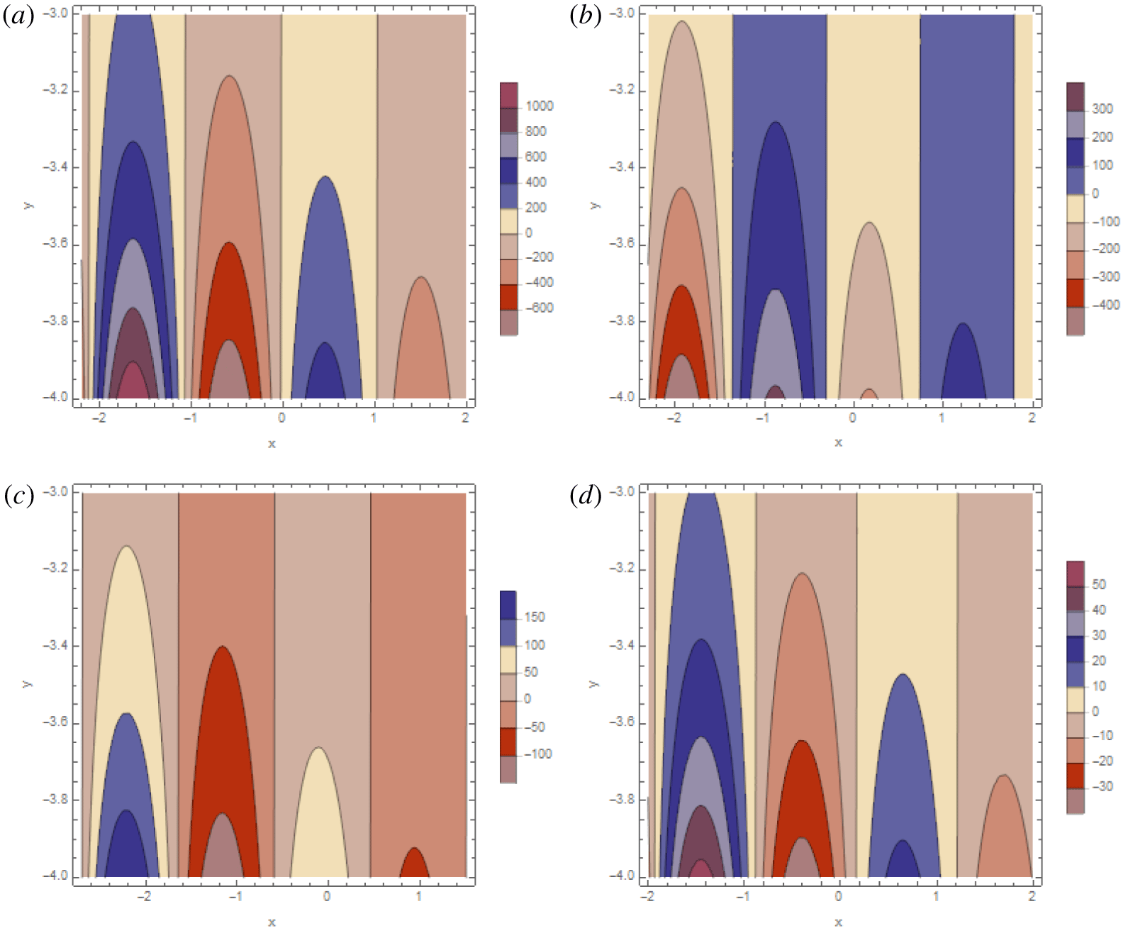
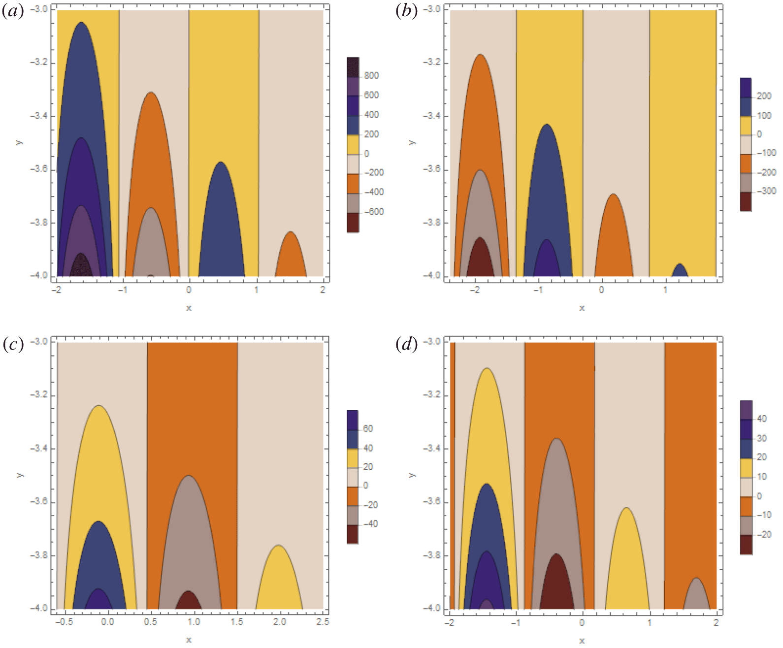
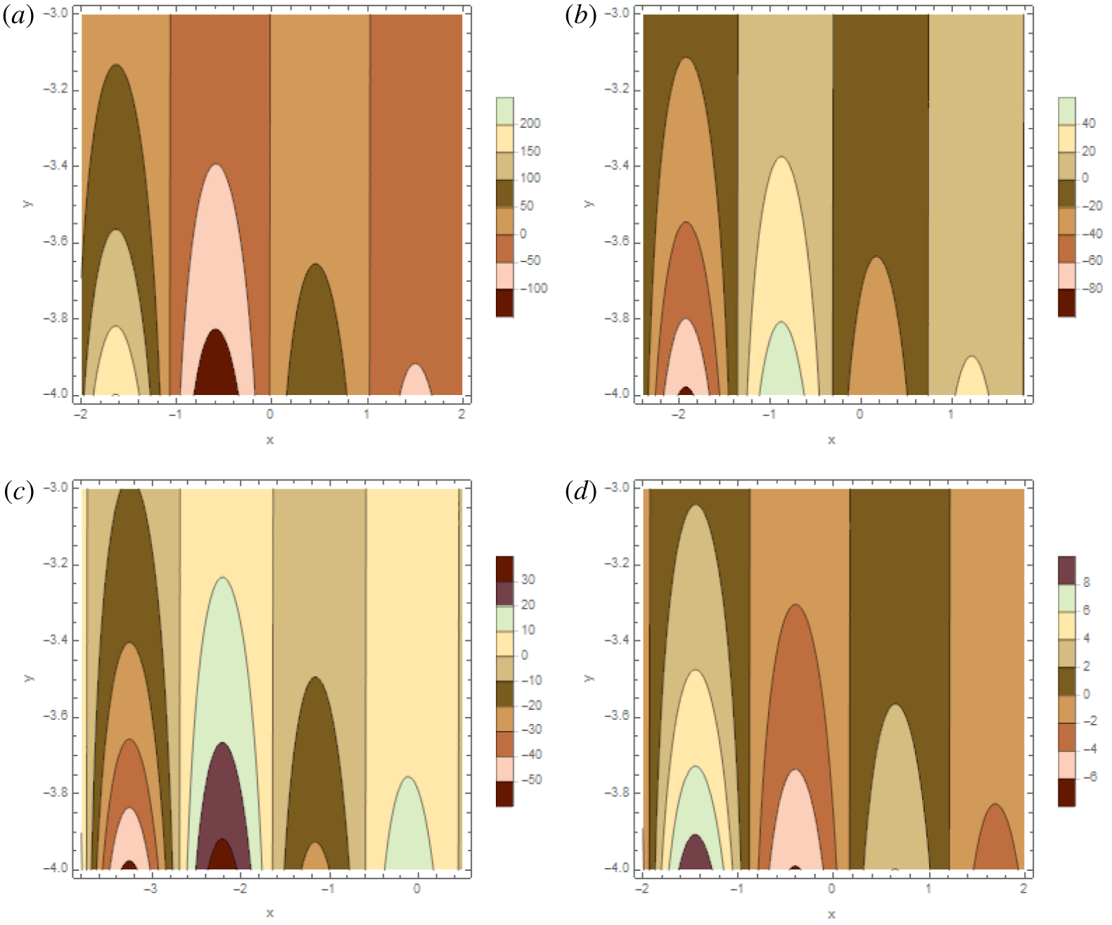
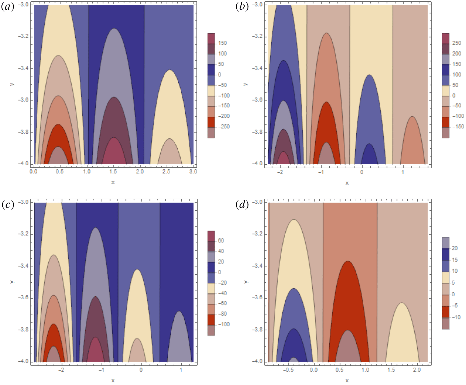
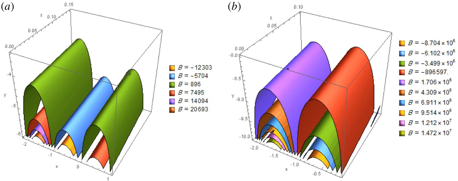
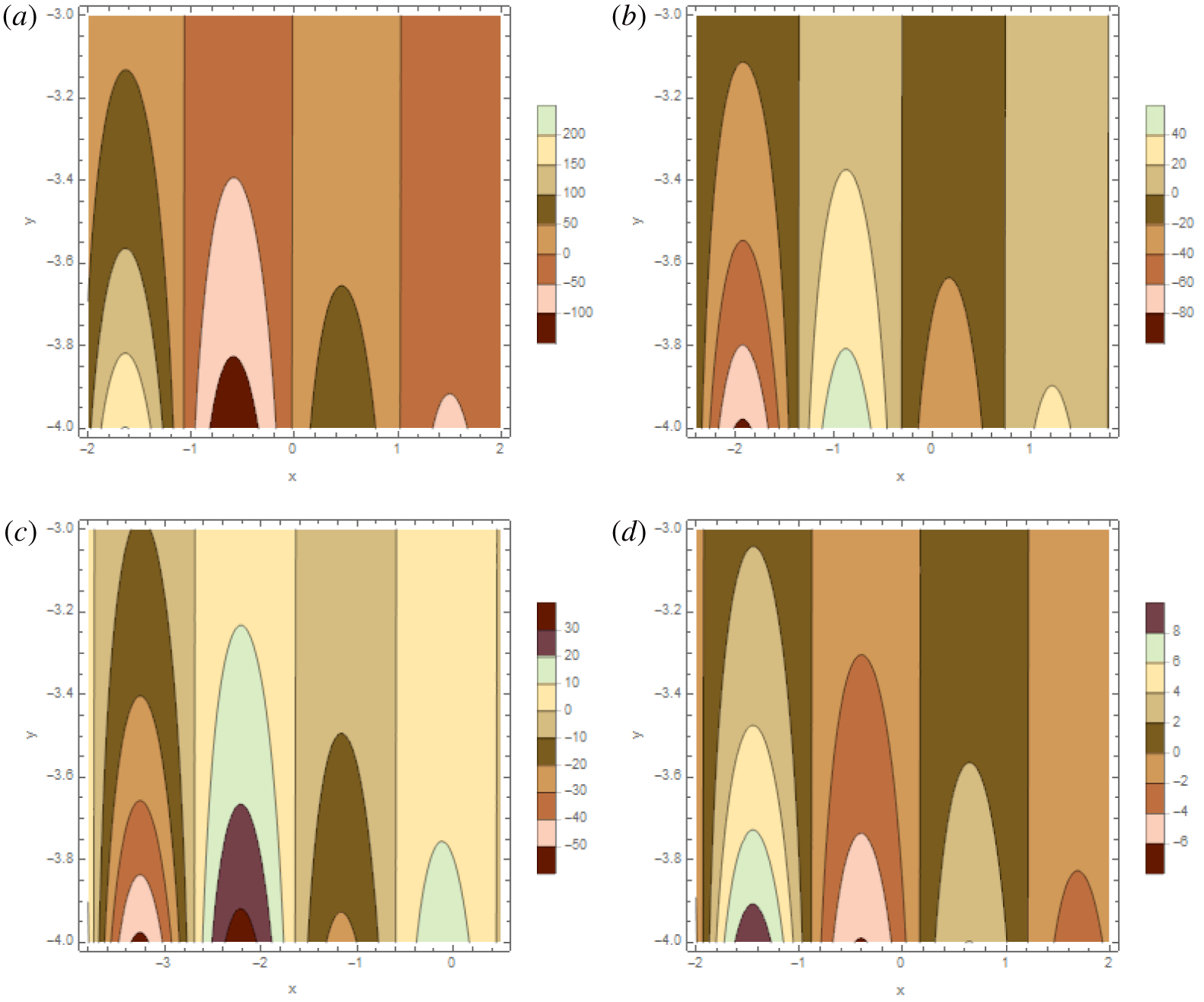
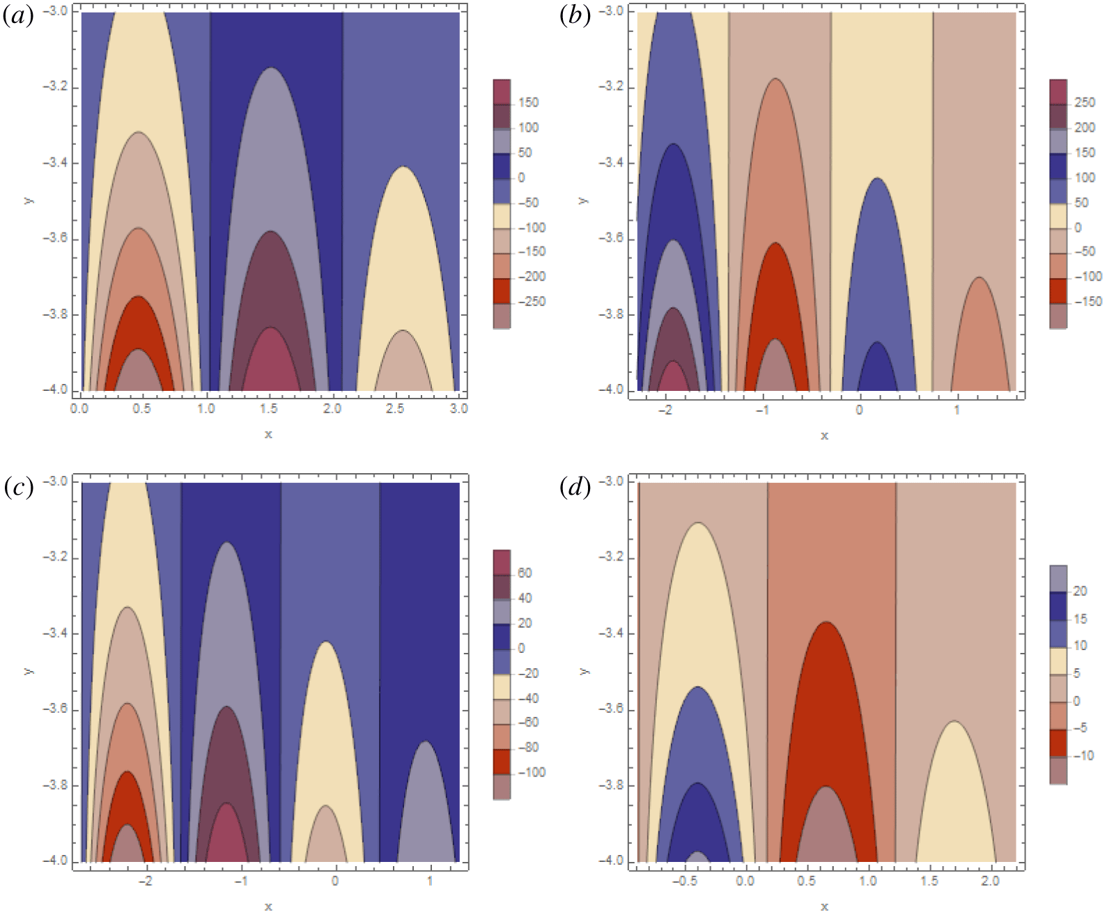
We are now testing the possibility of applying the resulting solution to astrophysics. Figures 1–4 with the values of the parameters listed in their captions show the magnetic field structures described by (5.6).

Figure 1.

Coronal loops of magnetic field lines for solution (5.6). The quantity plotted is the magnitude of the magnetic field vector shown in (5.6) for $z=0,1,2,3$. The loops are associated with places of strong magnetic fields like those on the Sun’s surface, where powerful magnetic fields break through the photosphere layer and extend into the Sun’s atmosphere. The values of parameters used are $a_{1}=-0.2$, $a_{2}=-0.8$, $a_{3}=-0.5$, $b_{1}=1.5$, $b_{2}=-0.01$, $b_{3}=2$.

Figure 2.

Contour plots of the $B_{x}$ component of the magnetic field described by solution (5.6) for $z=0,1,2,3$. The $x$-component of the vector $\bar{\boldsymbol{A}}$ is used as $\bar{A}_{1}=a_{3}b_{2}-a_{2}b_{3}=1.605$.

Figure 3.

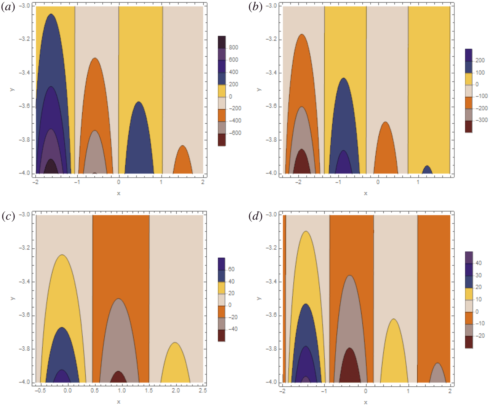
Contour plots of the $B_{y}$ component of the magnetic field described by solution (5.6) for $z=0,1,2,3$. The $y$-component of the vector $\bar{\boldsymbol{A}}$ is used as $\bar{A}_{2}=a_{1}b_{3}-a_{3}b_{1}=0.35$.

Figure 4.

Contour plots of the $B_{z}$ component of the magnetic field described by solution (5.6) for $z=0,1,2,3$. The $z$-component of the vector $\bar{\boldsymbol{A}}$ is used as $\bar{A}_{3}=a_{2}b_{1}-a_{1}b_{2}=-1.202$.

The behaviour of the above solutions (5.2) and (5.6) can be investigated at infinity as follows. Since the trigonometric functions $\sin (b_{1}x+b_{2}y+b_{3}z)$ and $\cos (b_{1}x+b_{2}y+b_{3}z)$ are bounded, where their ranges lie in the closed interval $[-1,1]$, hence $\boldsymbol{v}\longrightarrow 0$ when $x\longrightarrow \infty$, $y\longrightarrow y_{0}$ and $z\longrightarrow z_{0}$. Also, $\boldsymbol{B}\longrightarrow 0$ when $x\longrightarrow \infty$, $y\longrightarrow y_{0}$ and $z\longrightarrow z_{0}$. Similarly, when $y\longrightarrow \infty$, $x\longrightarrow x_{0}$ and $z\longrightarrow z_{0}$ and when $z\longrightarrow \infty$, $x\longrightarrow x_{0}$ and $y\longrightarrow y_{0}$, we find that the above solutions are bounded. When $x$, $y$ or $z\longrightarrow -\infty$, one can use positive values of the constants $a_{1},a_{2}$ and $a_{3}$ for bounded solutions. Therefore, all the solutions are bounded at infinity in which they are physically acceptable and suitable for astrophysics and the solar magnetic field.

Figure 5.

(a) Three-dimensional contour plots of the magnetic field lines of solution (5.6). The quantity plotted is the magnitude of the magnetic field vector shown in (5.6). The plots show loops rooted in sunspots, arcing between pairs of sunspots with opposite magnetic poles. (b) The magnetic energy corresponding to the magnetic field lines.

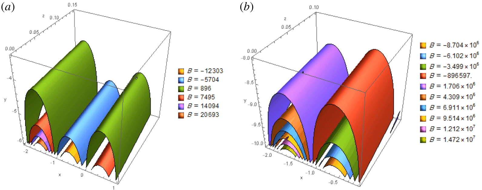
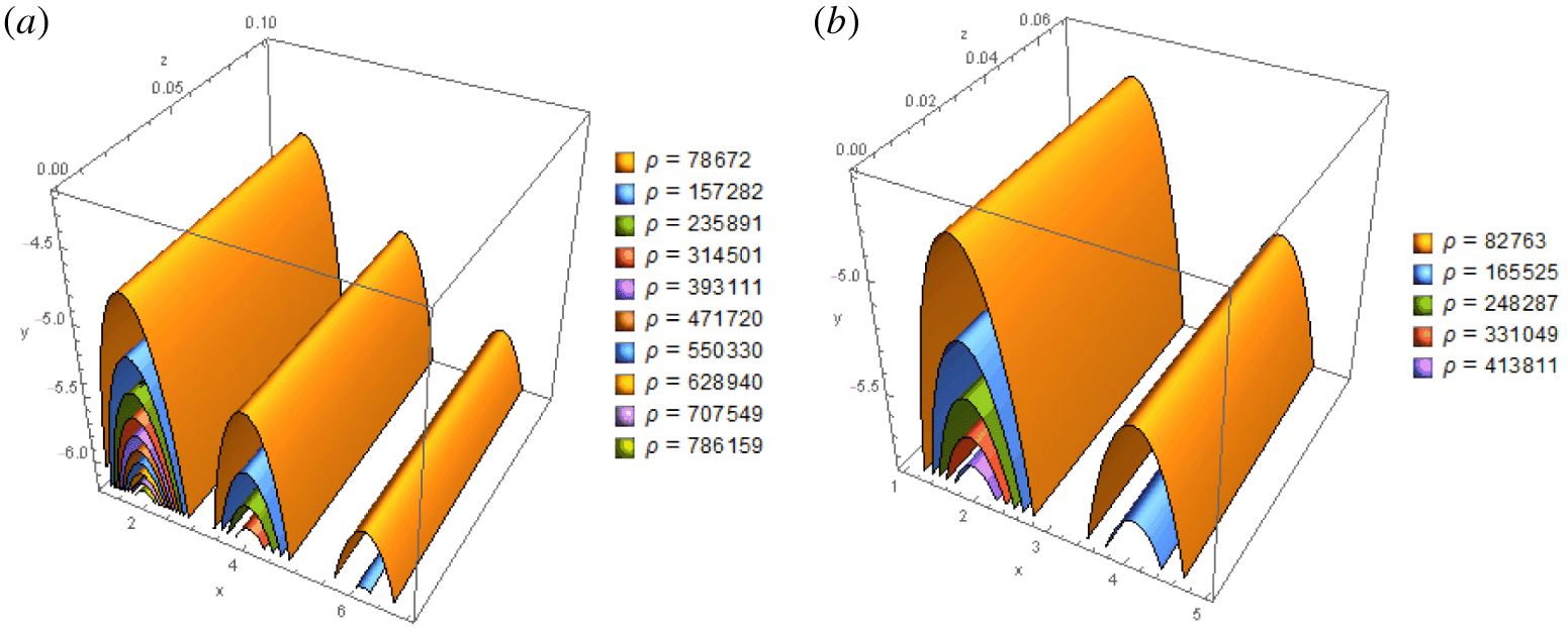
Figures 1–4 show curved structures that appear as arcs resembling the coronal loops above the Sun’s surface. The electrified plasma flows along the curved lines of a powerful magnetic field, giving the coronal loops their unique shapes. The configuration of the magnetic field lines and their components is characterized by the fact that the magnetic flux extends upward from one point and then extends down to another point, forming a pair of hot plasma arcs, such as sunspots. The three-dimensional contour of these configurations is shown in figure 5(a). It indicates that the magnetic flux extends from one pole up to the corona and then down to the other pole. Thus, the above solution may describe a gaseous plasma extending outward from the surface of the Sun, such as solar prominences, which rises from the photosphere through the chromosphere. These gigantic gas plumes are usually loop shaped and are the most spectacular of the solar phenomena. The magnetic energy shown in figure 5(b) appears to be concentrated at some point in the horizontal plane, indicating the direction along the photosphere layer. The magnetic energy increases to the left of some points (below the top of the graph) and then it is reduced to the right of these points. The portion in the $yz$-plane below the top of the graph of figure 5(b) represents a strong magnetic field region, which is considered to form solar prominences. The change in density and pressure of the plasma between the photosphere and the chromosphere region is shown in figures 6(a) and 6(b).

Figure 6.

Three-dimensional contour plots show the change of the density in (a) and pressure in (b) of magnetic field lines for solution (5.6). The values of parameters used are $a_{1}=-0.2$, $a_{2}=-0.8$, $a_{3}=-0.5$, $b_{1}=1.5$, $b_{2}=-0.01$, $b_{3}=2$, $\unicode[STIX]{x1D6EC}=1$, $\unicode[STIX]{x1D707}=0.01$, $K_{0}=1000$. The quantity $A$ appearing in (5.9) reads $A=-a_{3}^{2}(b_{1}^{2}+b_{2}^{2})+2a_{1}a_{3}b_{1}b_{3}+2a_{2}b_{2}(a_{1}b_{1}+a_{3}b_{3})-a_{2}^{2}(b_{1}^{2}+b_{3}^{2})-a_{1}^{2}(b_{2}^{2}+b_{3}^{2})=-4.14333$.

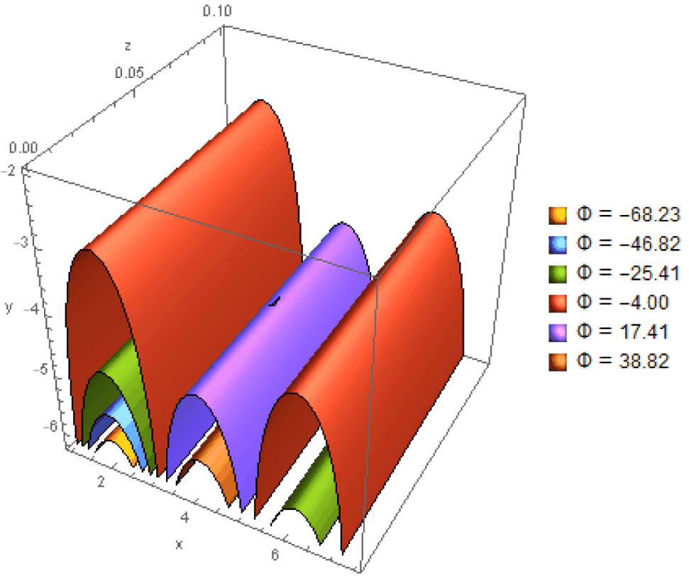
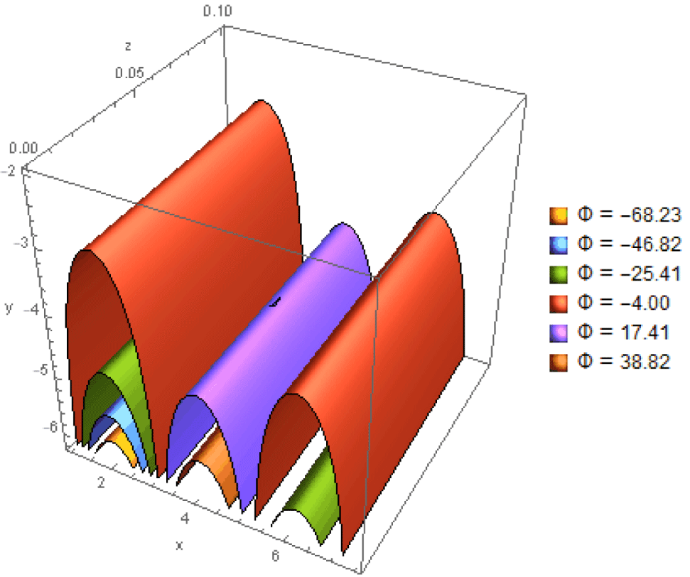
When dealing with gravitational potential energy at long distances, we usually choose a zero-point position that appears to be counterintuitive. We place the zero point of the gravitational potential energy at an infinite distance $r$. The formulation of the potential is shown in (5.5). It is very convenient to describe the energy requirements for travelling between different bodies in the solar system. This potential change is shown in figure 7.

Figure 7.

The three-dimensional contour graphs show prominences formed by the magnetic field, forming loops with each end anchored to the photosphere layer of the Sun’s surface. The parameter values are the same as those used in figure 6.

The above class of solutions has physical features relevant to the general appearance of quiescent prominences occurring at the base of coronal streamers as long-lasting cool sheets of matter in the hot corona surrounding. It may be of interest for describing coronal field structures of arcade-type magnetic fields originating from the photosphere between magnetic places of opposite polarity. It can describe the closed-type dipole configuration of the field penetration pre-active phase.

The magnetospheric boundaries of the Earth along the flanks can be unstable to Kelvin–Helmholtz instability under northward interplanetary magnetic field conditions. This instability can cause surface waves on the flank of the magnetopause that can facilitate the transportation of solar wind plasma into the Earth’s magnetosphere (Nykyri & Otto Reference Nykyri and Otto2001; Matsumoto & Hoshino Reference Matsumoto and Hoshino2004; Nakamura & Fujimoto Reference Nakamura and Fujimoto2008; Rossi et al. Reference Rossi, Califano, Retin, Sorriso-Valvo, Henri, Servidio, Valentini, Chasapis and Rezeau2015).

Rolled-up vortices like waves occurring on the Earth’s magnetopause and that allow plasma transport within the magnetosphere are shown in (5.3). Kelvin–Helmholtz instability can describe the formation of these vortices. At the Earth’s magnetopause, the Kelvin–Helmholtz waves are characterized by quasi-periodic fluctuations of the parameters of the plasma and magnetic field Lu et al. (Reference Lu, Wang, Li, Tang, Torbert, Giles, Russell, Burch, Mcfadden and Auster2019). The above class of solutions has this characterization. For several decades, the penetration of solar wind plasma across the magnetopause into the magnetosphere of the Earth has been the subject of study. In a magnetotail-like geometry, Takagi et al. (Reference Takagi, Hashimoto, Hasegawa, Fujimoto and Tandokoro2006) performed three-dimensional MHD simulations of Kelvin–Helmholtz instability. They found that rolled-up vortices had a characteristic feature when relating speed and density, showing a component of low-density plasma with tailward speeds exceeding that of the adjacent magnetosheath flow, and suggested that this feature could be used as a marker of Kelvin–Helmholtz roll-up driven vortices. Hasegawa et al. (Reference Hasegawa, Fujimoto, Takagi, Saito, Mukai and Rème2006) reported observations of spacecraft similar to the three-dimensional MHD simulation results by Takagi et al. (Reference Takagi, Hashimoto, Hasegawa, Fujimoto and Tandokoro2006). In the solar atmosphere, numerous instabilities have been reported. Ryutova et al. (Reference Ryutova, Berger, Frank, Tarbell and Title2010) found plumes on the boundary between a cavity and the prominence above it. They interpreted these to be the consequence of the Rayleigh–Taylor instability. Berger, Liu & Low (Reference Berger, Liu and Low2012) found vortex structures on the flank of such plumes, which are common features of the Kelvin–Helmholtz instability (Hillier et al. Reference Hillier, Isobe, Shibata and Berger2012).

Thus, the class of the solutions presented here may be of interest in describing magnetopause Kelvin–Helmholtz waves rich in magnetic and flow structures which are key to understanding the role of these waves in facilitating the transport of the solar wind plasma into the Earth’s magnetosphere. However, the presented solutions are not appropriate for describing isentropic plasma dynamics, such as (a) the magnetopause’s short-wavelength stability between a fast rotating, supersonic, dense accretion disk and a magnetized star’s slowly rotating low-density magnetosphere, (b) the case of a star with an aligned dipole magnetic field so that the magnetic field is axial in the disc mid-plane and perpendicular to the disc flow velocity.