1. Introduction
The gravity-driven settling of particles is widely encountered in environmental and industrial applications (Guazzelli & Hinch Reference Guazzelli and Hinch2011; Brandt & Coletti Reference Brandt and Coletti2022). Examples include precipitations in the atmosphere (Pruppacher & Klett Reference Pruppacher and Klett2010), the marine snow of settling plankton or debris (Trudnowska et al. Reference Trudnowska, Lacour, Ardyna, Rogge, Irisson, Waite, Babin and Stemmann2021), the deposition of ashes after a volcanic eruption (Rossi et al. Reference Rossi, Bagheri, Beckett and Bonadonna2021), and reacting particles in fluidized beds (Zhou et al. Reference Zhou, Pinson, Zou and Yu2011). Despite the relatively simple configurations often investigated, the problem is inherently complex and determined by several parameters, such as particle size, density and shape, as well as the fluid and flow characteristics. From a fundamental viewpoint, the settling rate and dynamics of the particle phase, and the particle-induced modulation of the underlying flows, which involve complicated interactions between a large number of settling particles and the carrier fluid flows, are highly relevant in the aforementioned applications and have therefore been the object of several studies (Batchelor Reference Batchelor1972; Caflisch & Luke Reference Caflisch and Luke1985; Guazzelli & Hinch Reference Guazzelli and Hinch2011; Brandt & Coletti Reference Brandt and Coletti2022).
Concerning the settling motion of multiple spheres in suspensions, many studies have been performed in the past decades. Among these, we recall the pioneering work by Richardson & Zaki (Reference Richardson and Zaki1954), who proposed the well-known idea of hindered settling of particles in the Stokes flow regime. Specifically, the upward mean flow, arising to compensate the particle downward motion, increases the total drag forces experienced by particles, so as to reduce their mean settling speed (Di Felice Reference Di Felice1999). As no analytical expression can be found even for monodisperse spheres, many efforts have been made to improve the empirical correlation of the hindered settling velocity as a function of the particle volume fraction and settling Reynolds number (Garside & Al-Dibouni Reference Garside and Al-Dibouni1977; Di Felice Reference Di Felice1999; Yin & Koch Reference Yin and Koch2007). Moreover, when the particle and fluid inertia become relevant, an enhancement of the particle settling speed in suspensions was initially reported by Kajishima & Takiguchi (Reference Kajishima and Takiguchi2002) and Kajishima (Reference Kajishima2004). Since then, with the help of particle-resolved direct numerical simulation (PR-DNS), the enhanced settling rate of particles has been related to the formation of column-like clusters in dilute suspensions provided that the settling Reynolds number is high enough (approximately greater than 175) (Uhlmann & Doychev Reference Uhlmann and Doychev2014; Zaidi et al. Reference Zaidi, Tsuji and Tanaka2014; Zaidi Reference Zaidi2018; Shajahan & Breugem Reference Shajahan and Breugem2023). These findings were also confirmed by the experiments conducted by Huisman et al. (Reference Huisman, Barois, Bourgoin, Chouippe, Doychev, Huck, Morales, Uhlmann and Volk2016).
The formation of particle clusters is attributed to the hydrodynamic interactions among settling spheres (Zaidi et al. Reference Zaidi, Tsuji and Tanaka2014). In particular, we recall the drafting–kissing–tumbling (DKT) interactions (Fortes et al. Reference Fortes, Joseph and Lundgren1987) between a pair of initially vertically aligned settling spheres. In this configuration, the rear particle, located in the wake of the leading one, experiences downward flows and thus accelerates its settling motion, which results in an attraction of the two spheres (drafting stage). Then the two particles touch and form an elongated body aligning vertically (kissing stage). Finally, as the elongated configuration is unstable, the two particles tumble under the effect of fluid inertia, and separate rapidly afterwards (tumbling stage). Similarly, in a suspension with multiple settling particles, the attraction and entrapment of particles in the wakes of upstream particles give rise to the formation of particle clusters with column-like arrangements (Uhlmann & Doychev Reference Uhlmann and Doychev2014; Zaidi et al. Reference Zaidi, Tsuji and Tanaka2014). As the consequence of the settling velocity of particle clusters being greater than that of the isolated particle, the mean settling rate of particles in the suspension can be enhanced substantially.
In the practical applications, particles are often non-spherical in shape, so they are commonly modelled as spheroids in earlier studies (Voth & Soldati Reference Voth and Soldati2017). Compared to the well-studied cases of settling spherical particles, less is known about the settling of non-spherical particles, especially in the finite-fluid-inertia regime. In Fornari et al. (Reference Fornari, Ardekani and Brandt2018), the settling of oblate particles with aspect ratio (the ratio between the polar and equator axes)
 $1/3$
and different volume fractions was investigated numerically. It was demonstrated that oblate particles can form notable clusters even at a relative low settling Reynolds number (approximately 40), leading to a significant enhancement of the mean settling velocity. The difference compared to the cases of settling spheres is ascribed to the stable piled-up structures of a pair of settling oblate spheroids undergoing DKT interactions (Ardekani et al. Reference Ardekani, Costa, Breugem and Brandt2016). Similarly, Moriche et al. (Reference Moriche, Hettmann, García-Villalba and Uhlmann2023) considered particles with a lower non-sphericity, aspect ratio
 $2/3$
, and reported that the easier attraction between settling oblate spheroids induces large-scale particle clusters with a long extension along the vertical direction. More recently, we studied the settling of prolate particles with aspect ratio 3 over a wide range of volume fractions from
 $0.1\,\%$
to
 $10\,\%$
, and found a non-monotonic variation of the particle settling velocity as the volume fraction increases (Jiang et al. Reference Jiang, Xu and Zhao2024b
). This phenomenon was explained by the combined effects of particle clustering, changes in orientation and the fluid hindrance on the settling motion of particle swarms.
From another point of view, the fluid flow induced by the gravity-driven motion of a dispersed phase is also a hot spot in the community of multiphase flow research. For example, the bubble-induced agitation generates a complex spatiotemporal flow, so-called pseudo-turbulence (Risso Reference Risso2018), which has been widely studied by experiments (Lance & Bataille Reference Lance and Bataille1991; Riboux et al. Reference Riboux, Risso and Legendre2010; Roghair et al. Reference Roghair, Mercado, van Sint Annaland, Kuipers, Sun and Lohse2011) and numerical simulations (Innocenti et al. Reference Innocenti, Jaccod, Popinet and Chibbaro2021; Hidman et al. Reference Hidman, Ström, Sasic and Sardina2023; Pandey et al. Reference Pandey, Ramadugu and Perlekar2020, Reference Pandey, Mitra and Perlekar2023). Unlike canonical turbulence where the energy is injected into the system by the large-scale flow shear, the pseudo-turbulence gains energy from the dispersed bubbles (Risso Reference Risso2018) with three features. First, it is anisotropic with larger fluctuations of vertical velocity than those of the horizontal component (Riboux et al. Reference Riboux, Risso and Legendre2010; Amoura et al. Reference Amoura, Besnaci, Risso and Roig2017). Second, the probability density function (p.d.f.) of the velocity fluctuation is non-Gaussian, with a skewed distribution of the vertical velocity fluctuations and exponential tails for the p.d.f. of the horizontal velocity fluctuations (Martínez-Mercado et al. Reference Martínez-Mercado, Palacios-Morales and Zenit2007; Riboux et al. Reference Riboux, Risso and Legendre2010). Third, the energy spectra is characterized by a
 $\kappa ^{-3}$
(where
 $\kappa$
is the wavenumber) power-law scaling on the scale comparable to or smaller than the bubble size (Lance & Bataille Reference Lance and Bataille1991; Martínez-Mercado et al. Reference Martínez-Mercado, Palacios-Morales and Zenit2007; Roghair et al. Reference Roghair, Mercado, van Sint Annaland, Kuipers, Sun and Lohse2011; Innocenti et al. Reference Innocenti, Jaccod, Popinet and Chibbaro2021), rather than the classical
 $\kappa ^{-5/3}$
power law of the single-phase turbulence. In Lance & Bataille (Reference Lance and Bataille1991), the
 $\kappa ^{-3}$
power law of the energy spectra was explained by the assumption of local balance between the energy production and dissipation in the wake of the rising bubbles. Recently, Pandey et al. (Reference Pandey, Mitra and Perlekar2023) reported the co-existence of Kolmogorov turbulence (the
 $\kappa ^{-5/3}$
power law) and pseudo-turbulence in the bubble-induced turbulence (the
 $\kappa ^{-3}$
power law), provided that the Reynolds number of the rising bubbles is sufficiently high.
However, the pseudo-turbulence induced by the interactions between heavy particles and a carrier fluid has received less attention so far. Mehrabadi et al. (Reference Mehrabadi, Tenneti, Garg and Subramaniam2015) numerically investigated the fluid flows past fixed or freely moving particle assemblies. They found that the degree of anisotropy in the Reynolds stresses depends on the volume fraction and the Reynolds number based on the mean slip velocity, and the mobility of the dispersed particles can influence the intensity of the pseudo-turbulence. Using point-particle DNS, Capecelatro et al. (Reference Capecelatro, Desjardins and Fox2014, Reference Capecelatro, Desjardins and Fox2015) investigated the gravity-driven motion of particles in an initially still fluid. The two-way coupling between the two phases leads to the local accumulation of settling particles (with particle Reynolds number
 $Re_p \sim O(1)$
), which in turn generates and sustains turbulence in the fluid phase. Concerning the finite-size particles, the fluid flow induced by settling particles was also studied primarily in the initially turbulent or quiescent environment (Fornari et al. Reference Fornari, Ardekani and Brandt2018, Reference Fornari, Zade, Brandt and Picano2019). It was reported that the particle-induced turbulence is anisotropic with unequal velocity fluctuations for different velocity components.
Inspired by the above literature review, we aim to investigate the characteristics of pseudo-turbulence in suspensions of settling particles. In particular, we are interested in how the presence of particle clustering influences the features of the particle-induced pseudo-turbulence. To this end, we perform PR-DNS of settling particles with three different shapes, i.e. oblate spheroids, spheres and prolate spheroids. We find that non-spherical particles, especially settling oblate spheroids, are prone to form column-like clusters in the suspension. As for the fluid phase, we identify a robust
 $\kappa ^{-3}$
power-law scaling in the energy spectrum of the particle-induced turbulent flows. Moreover, we find that the energy transfer in this kind of fluid flow is significantly affected by the particle clustering, which is found to enhance the energy input at large scales, facilitate the nonlinear transfer among scales, and promote energy redistribution to reduce the anisotropy of the pseudo-turbulence.
The remainder of this paper is organized as follows. In § 2, we introduce the flow configuration of this study, describe the numerical method of the PR-DNS based on the immersed boundary method, and introduce the observables in this study. In § 3, we focus on the collective behaviour of the dispersed phase, discussing the shape effect on the settling velocity and clustering of the particles. We concentrate on the turbulent flow induced by the settling particles in § 4, reporting the basic statistics of the fluid velocity fluctuations, and investigating the energy spectra and the budget of the turbulence kinetic energy. Finally, we summarize the key findings and draw conclusions in § 5.
2. Methodology
2.1. Flow configuration and parameter setting
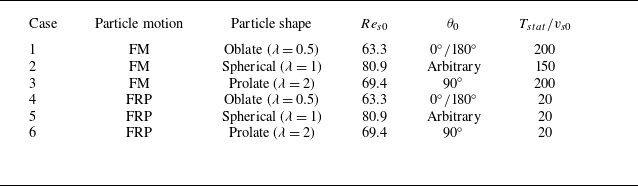
In the present work, we numerically study the sedimentation of spheroidal particles in a triply periodic domain filled with initially quiescent fluid (figure 1
a). The shape of the spheroidal particles is described by the aspect ratio
 $\lambda =a/b$
, where
 $a$
and
 $b$
denote the polar and equatorial radii of the spheroid, as shown in figure 1(b–d). The solid volume fraction, defined by
 $\phi = ({{\unicode{x03C0}} }/{6})(N_pD_{eq}^3)/(L_x L_y L_z)$
, is set to
 $\phi =1\,\%$
. This corresponds to
 $N_p=3129$
particles in a computational domain with size
 $L_x\times L_y \times L_z=32D_{eq} \times 160 D_{eq} \times 32D_{eq}$
, where
 $D_{eq}$
is the equivalent diameter of the particle (the diameter of a sphere with the same volume as the spheroid). The gravity is applied in the negative
 $y$
direction, and the ratio between the gravitational force and the viscous force is measured by the Galileo number
 $Ga=\sqrt {(\gamma -1)\,\|\boldsymbol{g}\|\,D_{eq}^3}/\nu$
. Here,
 $\gamma =\rho _p/\rho _f$
is the density ratio between particle and fluid,
 $\boldsymbol{g}$
is the gravitational acceleration, and
 $\nu$
is the kinematic viscosity of the fluid. In the present study, we set the Galileo number as
 $Ga=80$
, and consider settling particles with different shapes. The choice of this dimensionless parameter is motivated by the different DKT interactions for pairwise settling spheroids with different shapes at
 $Ga=80$
(Ardekani et al. Reference Ardekani, Costa, Breugem and Brandt2016). The particle–fluid density ratio is set as
 $\gamma =2$
, which is a typical value for the solid–liquid scenario (Seyed-Ahmadi & Wachs Reference Seyed-Ahmadi and Wachs2021). In total, we consider six simulation cases with three kinds of spheroidal particles: oblate particles with
 $\lambda =0.5$
, spherical particles with
 $\lambda =1$
, and prolate particles with
 $\lambda =2$
, as listed in table 1. With these parameter set-ups, we observe a significant clustering for freely moving oblate and prolate particles in the suspension (see the discussion in § 3.3). We note that the full decorrelation of the vertical fluid velocity is not attained when particle clustering occurs. Similar finite correlations were also reported in previous studies on settling particles (Uhlmann & Doychev Reference Uhlmann and Doychev2014; Moriche et al. Reference Moriche, Hettmann, García-Villalba and Uhlmann2023), and are difficult to eliminate by only increasing the size of the computational domain. Considering the limited influence of the domain size on the behaviour of settling particles (Zaidi Reference Zaidi2021) and the computational cost, we do not further enlarge the domain size in the current simulations. Additionally, as the reference cases, we simulate the settling of an isolated spheroid before conducting the simulations of multiple particles, and obtain the settling Reynolds number
 $Re_{s0}=v_{s0}D_{eq}/\nu$
for each type of particle (see table 1). Owing to the relatively low Reynolds number for the particle settling motion under the present parameter set-up, the rear wake of the isolated settling particle remains stable, so the path instability is not triggered (Jenny et al. Reference Jenny, Duek and Bouchet2004; Ern et al. Reference Ern, Risso, Fabre and Magnaudet2012). Additionally, we find in the simulation that the isolated settling oblate/prolate spheroid reorients with the major axis perpendicular to the gravitational direction, although a random inclined orientation is prescribed as the initial condition, due to the effect of fluid inertial torque (Ardekani et al. Reference Ardekani, Costa, Breugem and Brandt2016). Moreover, we also perform simulations of settling particles with fixed relative positions and frozen orientations; see table 1. The objective of these artificial simulations is to clarify the effect of particle clustering on the particle-induced turbulence, which is elaborated in § 4.
(a) Schematic representation of the sedimentation of spheroidal particles in a quiescent fluid. Three different shapes of particle are considered: (b) oblate particles with aspect ratio
 $\lambda =0.5$
; (c) spherical particles with
 $\lambda =1$
; and (d) prolate particles with
 $\lambda =2$
. The angle
 $\theta$
represents the angle between the vertical direction and the symmetry axis of the spheroid (denoted by
 $\boldsymbol{n}$
).

Set-ups for the simulation cases considered in the present study. The cases with freely moving particles are denoted by ‘FM’, while ‘FRP’ represents particles with fixed relative positions. The settling Reynolds number and the pitch angle for the isolated settling spheroid are denoted by
 $Re_{s0}$
and
 $\theta _0$
, respectively.

In each simulation, particles are initially seeded with random orientations and random positions in the computational domain, without overlaps. Readers can refer to Anoukou et al. (Reference Anoukou, Brenner, Hong, Pellerin and Danas2018) for the generation of initial particle assemblies. The statistics given in §§ 3 and 4 are obtained after the system has reached a fully developed state, which is ensured by monitoring the time evolution of the particle-averaged settling velocity in the simulation. The duration of the time window over which we compute the statistics, denoted by
 $T_{stat}$
, is provided in table 1. This time interval is extended for the cases with freely moving particles to allow for the organization of particle micro-structures in these cases.
2.2. Fluid solver and immersed boundary method
The fluid flow is governed by the incompressible Navier–Stokes equations:
 \begin{align} &\qquad\qquad\quad \nabla {\,\boldsymbol\cdot\,} \boldsymbol{u} =0, \end{align}
 \begin{align} &\frac {\partial \boldsymbol{u}}{\partial t}+\boldsymbol{u} {\,\boldsymbol\cdot\,} \nabla \boldsymbol{u} =-\nabla p+ \frac {1}{Re} \nabla ^{2} \boldsymbol{u}+ \boldsymbol{f} . \end{align}
Here,
 $\boldsymbol{u}=(u,v,w)$
denotes the velocity of the fluid flow,
 $p$
is the pressure, and
 $\boldsymbol{f}$
is the immersed boundary (IB) forcing term (IB force). Note that (2.1)–(2.2) are presented in dimensionless form, and the Reynolds number
 $Re=U_0L_0/\nu$
is defined based on the characteristic velocity (
 $U_0$
) and length (
 $L_0$
) of the fluid flow. Here, we set the settling velocity of an isolated particle as the characteristic velocity and the equivalent diameter as the character length, i.e.
 $U_0=v_{s0}$
and
 $L_0=D_{eq}$
. The IB forces in (2.2) are employed to resolve the interactions between the rigid particles and the fluid flows (as elaborated in the following).
To solve (2.1)–(2.2) numerically, we adopt a fractional step method for the decoupling of velocity and pressure (Kim et al. Reference Kim, Baek and Sung2002). Using the Crank–Nicolson scheme for the temporal discretization of the convection and viscous terms, the temporal advancement of (2.1)–(2.2) from the
 $n$
th to the
 $(n+1)$
th time step is written as (Kim et al. Reference Kim, Baek and Sung2002)
 \begin{align} &\frac {\boldsymbol{u}^{*}-\boldsymbol{u}^{n}}{\Delta t}+\frac {1}{2}(H( \boldsymbol{u}^{*})+H( \boldsymbol{u}^{n})) = -G p^{n-1/2}+\frac {1}{2\, R e}\left (L \boldsymbol{u}^{*}+L \boldsymbol{u}^{n}\right ), \end{align}
 \begin{align} &\qquad\qquad\qquad\qquad\,\, \boldsymbol{u}^{**} = \boldsymbol{u}^* + \Delta t\,{\boldsymbol{f}}^{n + 1/2},_{_{_{_{}}}} \end{align}
 \begin{align} &\qquad\qquad\qquad\qquad\quad D G\, \delta p = D \boldsymbol{u}^{* *}/\Delta t, \end{align}
 \begin{align} &\qquad\qquad\qquad\qquad\,\, p^{n+1/2} = p^{n-1/2}+\delta p, \end{align}
 \begin{align} &\qquad\qquad\qquad\qquad\,\, \boldsymbol{u}^{n+1} = \boldsymbol{u}^{* *}-\Delta t\, G\, \delta p. \end{align}
Here,
 $H$
,
 $G$
,
 $L$
and
 $D$
represent the spatial discrete convection, gradient, Laplacian and divergence operators, which are evaluated by the central finite-difference scheme on a staggered Eulerian grid (Kim et al. Reference Kim, Baek and Sung2002). The first prediction velocity
 $\boldsymbol{u}^*$
is updated without considering the IB forces in (2.3). The second prediction velocity
 $\boldsymbol{u}^{**}$
is then computed by (2.4) with the introduction of IB forces. Finally, the velocity projection step is performed by solving the Poisson equation (2.5), updating the pressure as in (2.6), and updating the velocity by (2.7).
To impose the no-slip boundary condition on the particle surfaces, we employ the direct-forcing IB method to calculate the IB forces (Uhlmann Reference Uhlmann2005; Breugem Reference Breugem2012):
 \begin{align} &\quad\boldsymbol{U}^{*}_{l}=\sum \limits _{ijk} {{\boldsymbol{u}}_{ijk}^{*}\,\delta \left ( {\boldsymbol{X}^{n}_{l}}-{{\boldsymbol{x}}_{ijk}} \right )\,\Delta {h^3}}, \end{align}
 \begin{align} &\qquad\quad {\boldsymbol{F}}_{l}^{n+1/2} = \frac {{{{\boldsymbol{U}_p}(\boldsymbol{X}^{n}_{l})} - {\boldsymbol{U}}_{l}^{*}}}{{\Delta t}}, \end{align}
 \begin{align} &{\boldsymbol{f}}_{ijk}^{n + 1/2} = \sum \limits _{l} {{\boldsymbol{F}}_{l}^{n+1/2}\,\delta \left ( {{{\boldsymbol{x}}_{ijk}} - {\boldsymbol{X}^{n}_{l}}} \right )\Delta {V_{l}}}. \end{align}
Here, the capital letters refer to variables defined on the Lagrangian marker points allocated on the particle surface. In (2.8), the first prediction velocity
 $\boldsymbol{u}^*$
is interpolated from the Eulerian grid points to the Lagrangian marker points using the Dirac delta function
 $\delta ({\boldsymbol\cdot})$
, where
 $\boldsymbol{X}^n_l$
denotes the position of the
 $l$
th Lagrangian marker point. Then the IB force is obtained on the Lagrangian marker point from (2.9), with
 $\boldsymbol{U}_p$
representing the rigid-body velocity of the particle. Finally, the IB forces are spread onto the Eulerian grid with the Dirac delta function via (2.10), in which
 $\Delta V_l$
denotes the volume associated with the
 $l$
th Lagrangian marker point. The Dirac delta function presented in (2.8) and (2.10) is defined by
 \begin{equation} \delta \left ( {\boldsymbol{x}} \right ) = \frac {1}{{\Delta {h^3}}} \times \phi \left(\frac {x}{{\Delta h}}\right) \times \phi \left(\frac {y}{{\Delta h}}\right) \times \phi \left(\frac {z}{{\Delta h}}\right), \end{equation}
in which
 $\phi ({\boldsymbol\cdot})$
is a 3-grid-width discrete Dirac delta function (Roma et al. Reference Roma, Peskin and Berger1999):
 \begin{equation} \phi (r)=\begin{cases}\dfrac {1}{6}(5-3|r|-\sqrt {-3(1-|r|)^2+1)}, &\quad 0.5\leqslant |r|\leqslant 1.5, \\[8pt] \dfrac {1}{3}(1+\sqrt {-3r^2+1}), &\quad |r|\leqslant 0.5, \\[6pt] 0, &\quad \text{otherwise}.\end{cases} \end{equation}
In the present study, a uniform Eulerian grid with an equal spacing in the three directions, i.e.
 $\Delta h=\Delta x=\Delta y=\Delta z=D_{eq}/24$
, is utilized. This grid size has been validated to be fine enough to resolve the particle–fluid interaction in the simulation of the isolated settling particle. The time step for the simulation is set as
 $\Delta t=0.01 D_{eq}/v_{s0}$
for each case, leading to the Courant number (based on the isolated settling velocity)
 $CFL = 0.24$
. Furthermore, for the implementation of the direct-forcing IB method, we employ the multi-forcing scheme with
 $N_s=2$
iterations, and consider the inward retraction of Lagrangian marker points with distance
 $r_d=0.3\,\Delta h$
to better approximate the no-slip boundary condition on the particle surface (for more details, see Breugem Reference Breugem2012). Additionally, a zero flux constraint is imposed in the simulation by subtracting the spatially averaged IB forces after (2.10) at each time step (Chouippe & Uhlmann Reference Chouippe and Uhlmann2015; Höfler & Schwarzer Reference Höfler and Schwarzer2000):
 \begin{equation} {\boldsymbol{f}}_{ijk}^{n + 1/2}={\boldsymbol{f}}_{ijk}^{n + 1/2}-\langle {\boldsymbol{f}}_{ijk}^{n + 1/2} \rangle _{V}, \end{equation}
where the operator
 $\langle {\boldsymbol\cdot} \rangle _{V}$
represents the spatial average over the whole computational domain.
2.3. Particle motion
The motion of spheroidal particles in fluid flow is governed by the Newton–Euler equations:
 \begin{align} &\rho _{p} V_{p} \frac {\mathrm{d} \boldsymbol{v}}{\mathrm{d} t}=\boldsymbol{F}_{H}+\left (\rho _{p}-\rho _{f}\right ) \boldsymbol{g} V_{p}+\boldsymbol{F}_{C}, \end{align}
 \begin{align} &\qquad\qquad \frac {\mathrm{d} (\boldsymbol{I} {\,\boldsymbol\cdot\,} \boldsymbol{\omega })}{\mathrm{d} t}=\boldsymbol{T}_{H}+\boldsymbol{T}_{C}, \end{align}
where
 $V_p$
denotes the particle volume,
 $\boldsymbol{I}$
is the moment of inertia of the particle, and
 $\boldsymbol{v}=(v_x,v_y,v_z)$
and
 $\boldsymbol{\omega }$
represent the particle translational and angular velocities. In the framework of the direct-forcing IB method, the force and torque exerted from fluid flow onto the particle, denoted by
 $\boldsymbol{F}_H$
and
 $\boldsymbol{T}_H$
, can be computed by (Breugem Reference Breugem2012)
 \begin{align} &\quad\,\, {{\boldsymbol{F}}_H} = - {\rho _f}\sum_l {{{\boldsymbol{F}}_l}\,\Delta {V_l}} + {\rho _f}\,\frac {\mathrm{d}}{{\mathrm{d} t}}\int_{{V_p}} {{\boldsymbol{u}}\,{\rm d}V}, \end{align}
 \begin{align} &{{\boldsymbol{T}}_H} = - {\rho _f}\sum_l {{\boldsymbol{r}} \times {{\boldsymbol{F}}_l}\,\Delta {V_l}} + {\rho _f}\,\frac {\mathrm{d}}{{\mathrm{d} t}}\int_{{V_p}} {{\boldsymbol{r}} \times {\boldsymbol{u}}\,{\rm d}V} . \end{align}
Refer to our previous works (Jiang et al. Reference Jiang, Huang, Xu and Zhao2024a , Reference Jiang, Xu and Zhaob ) for more details and validations of the aforementioned numerical method to simulate the particle–fluid interactions.
Moreover, the contact force (
 $\boldsymbol{F}_{C}$
) and torque (
 $\boldsymbol{T}_{C}$
) are included to account for the particle–particle collisions. In detail, we consider the lubrication force based on the model of Jeffrey (Reference Jeffrey1982) when the surface-to-surface distance between two particles is smaller than one grid spacing, and apply the normal and tangential collision force based on the soft-sphere model for the touching particles (Costa et al. Reference Costa, Boersma, Westerweel and Breugem2015). More details about the implementation and validation of the contact force can be found in Costa et al. (Reference Costa, Boersma, Westerweel and Breugem2015) and Ardekani et al. (Reference Ardekani, Costa, Breugem and Brandt2016).
Note that in the simulations of settling particles with fixed relative positions, we calculate the average of the hydrodynamic forces over all particles, i.e. (the subscript
 $i$
refers to the particle counting)
 \begin{equation} \boldsymbol{F}_{H,avg}=\frac {1}{N_p}\sum \limits _{i = 1}^{{N_p}} {{{\boldsymbol{F}}_{H,i}}}, \end{equation}
and use
 $\boldsymbol{F}_{H,avg}$
to update the velocity of each particle in (2.14). In this manner, the particle velocities are identical so as to keep their initial relative positions without imposing a predefined settling speed. As regards the particle angular dynamics, (2.15) is not solved, so the orientation of the dispersed particles is frozen.
2.4. Data analysis
Here, we introduce the post-processing tools adopted in the present work. In particular, we use Voronoi analysis to examine particle clustering, and perform scale-by-scale budget analysis of the turbulent flow induced by the settling particles.
2.4.1. Voronoi analysis
In the present work, we examine the spatial distribution of dispersed particles by virtue of the Voronoi diagram (Monchaux et al. Reference Monchaux, Bourgoin and Cartellier2010). To quantify the clustering tendency, we define a dimensionless parameter, i.e. the clustering indicator
 $C$
, as (Tagawa et al. Reference Tagawa, Roghair, Prakash, van Sint Annaland, Kuipers, Sun and Lohse2013)
 \begin{equation} C=\sigma (\overline {V}_{Voro})/\sigma (\overline {V}_{Voro,rand}). \end{equation}
In the above definition,
 $\sigma (\overline {V}_{Voro})$
denotes the standard deviation of the normalized Voronoi volumes, and
 ${V}_{Voro,rand}$
represents the volume of tesselation for a random particle distribution. The normalized Voronoi volume of the
 $i$
th particle is defined by
 \begin{equation} \overline {V}_{Voro}(i)=\frac{V_{Voro}(i)}{V_{tot}/N_p}, \end{equation}
in which
 $V_{tot}=L_x L_y L_z$
denotes the volume of the entire computational domain. According to the definition in (2.19),
 $C\lt 1$
indicates that the particle spatial distribution is closer to an orderly lattice-like arrangement than a random distribution. Conversely, if
 $C\gt 1$
, then the system has a high tendency to clustering, with an increased number of regions with locally accumulated particles (clusters) and of empty regions (voids). Note that, unlike the case of point-particles (Ferenc & Néda Reference Ferenc and Néda2007), the p.d.f. of the Voronoi volumes for a random distribution of finite-size particles does not conform to a Poisson distribution (Uhlmann Reference Uhlmann2020). Thus to compute the clustering indicator
 $C$
by (2.19), we statistically obtain
 $\sigma (\overline {V}_{voro,rand})$
by repeatedly generating non-overlapping finite-sized particles with random positions (and also random orientations for non-spherical particles) (Anoukou et al. Reference Anoukou, Brenner, Hong, Pellerin and Danas2018).
2.4.2. Particle-induced turbulence: scale-by-scale budget
One objective of the present study is to understand the characteristics and energy transfer of the pseudo-turbulent flow (adopting the term used for the bubble-induced turbulence) induced by the settling particles. To this end, we will investigate the scale-by-scale energy budget of the particle-induced turbulent flow. Here, we briefly introduce the derivation of the fluid-phase energy budget equation in spectral space (see, among others, Crialesi-Esposito et al. Reference Crialesi-Esposito, Rosti, Chibbaro and Brandt2022). First, we take the Fourier transform of the
 $i$
th (
 $i=1,2,3$
) component of the momentum equation (2.2):
 \begin{equation} \frac {\partial \widetilde {u_i}}{\partial t}+\widetilde {G_i}=-\widetilde {P_i}+\widetilde {V_i}+\widetilde {f_i}. \end{equation}
Here,
 $G_i=u_j\,\partial u_i/\partial x_j$
,
 $P_i=(1/\rho _f)\, \partial p/\partial x_i$
and
 $V_i=\partial ^2 u_i/(\partial x_j\, \partial x_j)$
denote the nonlinear, pressure gradient and viscous terms, respectively. The notation
 $\tilde {g}(\boldsymbol{\kappa}, t)$
represents the Fourier mode at the wavenumber vector
 $\boldsymbol{\kappa} =(\kappa_x, \kappa_y, \kappa_z)$
of an arbitrary variable
 $g(\boldsymbol{x}, t)$
(g could be
 $u_i, G_i, P_i, V_i$
or
 $f_i$
) in the physical domain. Next, we multiply (2.21) with the complex conjugate of the velocity
 $\widetilde {u_i}^*$
, leading to (no summation over index
 $i$
)
 \begin{equation} \widetilde {u_i}^*\frac {\partial \widetilde {u_i}}{\partial t}+\widetilde {u_i}^*\widetilde {G_i}=-\widetilde {u_i}^*\widetilde {P_i}+\widetilde {u_i}^*\widetilde {V_i}+\widetilde {f}_i\widetilde {u_i}^*. \end{equation}
Taking the summation of (2.22) with its complex conjugate, we finally obtain the scale-by-scale budget equation for the
 $i$
th velocity component:
 \begin{equation} \frac {\partial \mathcal{E}_{i}\left (\boldsymbol{\kappa },t\right )}{\partial t}=\mathcal{T}_{i}\left (\boldsymbol{\kappa },t\right )+\mathcal{P}_{i}\left (\boldsymbol{\kappa },t\right )+\mathcal{D}_{i}\left (\boldsymbol{\kappa },t\right )+\mathcal{F}_{i}\left (\boldsymbol{\kappa },t\right ). \end{equation}
The physical interpretation of each term in (2.23) is as follows (without the use of Einstein’s summation convention here):
-
(i)
 $\mathcal{E}_{i} (\boldsymbol{\kappa },t )= ({1}/{2})\widetilde {u_i}\widetilde {u_i}^*$
is the energy of the velocity component
$u_i$
in the spectral domain
-
(ii)
$\mathcal{T}_{i} (\boldsymbol{\kappa },t )=-({1}/{2}) (\widetilde {u_i}^*\widetilde {G_i}+\widetilde {u_i}\widetilde {G_i}^* )$
is the energy transfer by the nonlinear term -
(iii)
$\mathcal{P}_{i} (\boldsymbol{\kappa },t )=-({1}/{2}) (\widetilde {u_i}^*\widetilde {P_i}+\widetilde {u_i}\widetilde {P_i}^* )$
is the energy redistribution by pressure -
(iv)
$\mathcal{D}_{i} (\boldsymbol{\kappa },t )=({1}/{2}) (\widetilde {u_i}^*\widetilde {V_i}+\widetilde {u_i}\widetilde {V_i}^* )$
is the viscous dissipation -
(v)
$\mathcal{F}_{i} (\boldsymbol{\kappa },t )=({1}/{2}) (\widetilde {f_i}\widetilde {u_i}^*+\widetilde {f_i}^*\widetilde {u_i} )$
is the work done by the IB forces (reflecting the particle–fluid interactions).


Note that in the fully developed stage, the statistical steady state is reached, so we can further compute the time average of (2.23): the time derivative vanishes, and
 $\mathcal{T}_i$
,
 $\mathcal{P}_i$
,
 $\mathcal{D}_i$
and
 $\mathcal{F}_i$
are in balance. For the sake of simplicity, we drop the independent variable
 $t$
to denote the time-averaged energy spectra of the budget terms hereafter. Accordingly, a generic quantity
 $\mathcal{J}$
(which could refer to
 $\mathcal{E}$
,
 $\mathcal{T}$
,
 $\mathcal{P}$
,
 $\mathcal{D}$
or
 $\mathcal{F}$
) in (2.23) is a function of the three-dimensional wavenumber vector
 $\boldsymbol{\kappa }$
. We can calculate a spherical shell integral of
 $\mathcal{J} ( {\boldsymbol{\kappa }} )$
to obtain a one-dimensional function (Hidman et al. Reference Hidman, Ström, Sasic and Sardina2023):
 \begin{equation} \mathcal{J}(\kappa )=\sum \limits _{\kappa -\frac {1}{2}\Delta \kappa \leqslant \left \| {\boldsymbol{\kappa }} \right \| \leqslant \kappa +\frac {1}{2}\Delta \kappa } { \mathcal{J}\left ( {\boldsymbol{\kappa }} \right )}/\Delta \kappa . \end{equation}
However, the particle-induced turbulence is anisotropic under the action of gravity (see § 4). In order to further analyse the directional information of the distribution of
 $\mathcal{J}$
in spectral space, we also calculate the average of
 $\mathcal{J}(\boldsymbol{\kappa })$
over the isotropic directions (on the horizontal plane), and express
 $\mathcal{J}$
in cylindrical coordinates (denoted by the superscript
 $C$
) as
 \begin{equation} \mathcal{J}^C\left ( {{\kappa _r},{\kappa _v}} \right ) = \frac {1}{N_S}\sum \limits _{{\kappa _r} - \frac {1}{2}\Delta {\kappa _r} \lt \kappa _r \leqslant {\kappa _r} + \frac {1}{2}\Delta {\kappa _r}} { \mathcal{J} \left ( {\boldsymbol{\kappa }} \right )} /\left ( {\Delta {\kappa _r}\,\Delta {\kappa _v}} \right ), \end{equation}
where
 $\kappa _v=\kappa _y$
and
 $\kappa _r=\sqrt {\kappa _x^2+\kappa _z^2}$
represent the vertical and radial (along the horizontal direction) wavenumbers, respectively. The number of samples satisfying
 ${\kappa _r} - ({1}/{2})\,\Delta {\kappa _r} \lt \kappa _r \leqslant {\kappa _r} + ({1}/{2})\,\Delta {\kappa _r}$
is denoted by
 $N_S$
, which varies with
 $\kappa _r$
.
3. Collective behaviour of the dispersed particles
3.1. Settling velocity
The first observable with which we are concerned is the mean settling speed of the particles in suspension. In this study, we define the settling velocity
 $v_s$
as the particle velocity along the gravitational direction, namely
 $v_s=-v_y$
, and we use the angle bracket
 $\langle {\boldsymbol\cdot} \rangle$
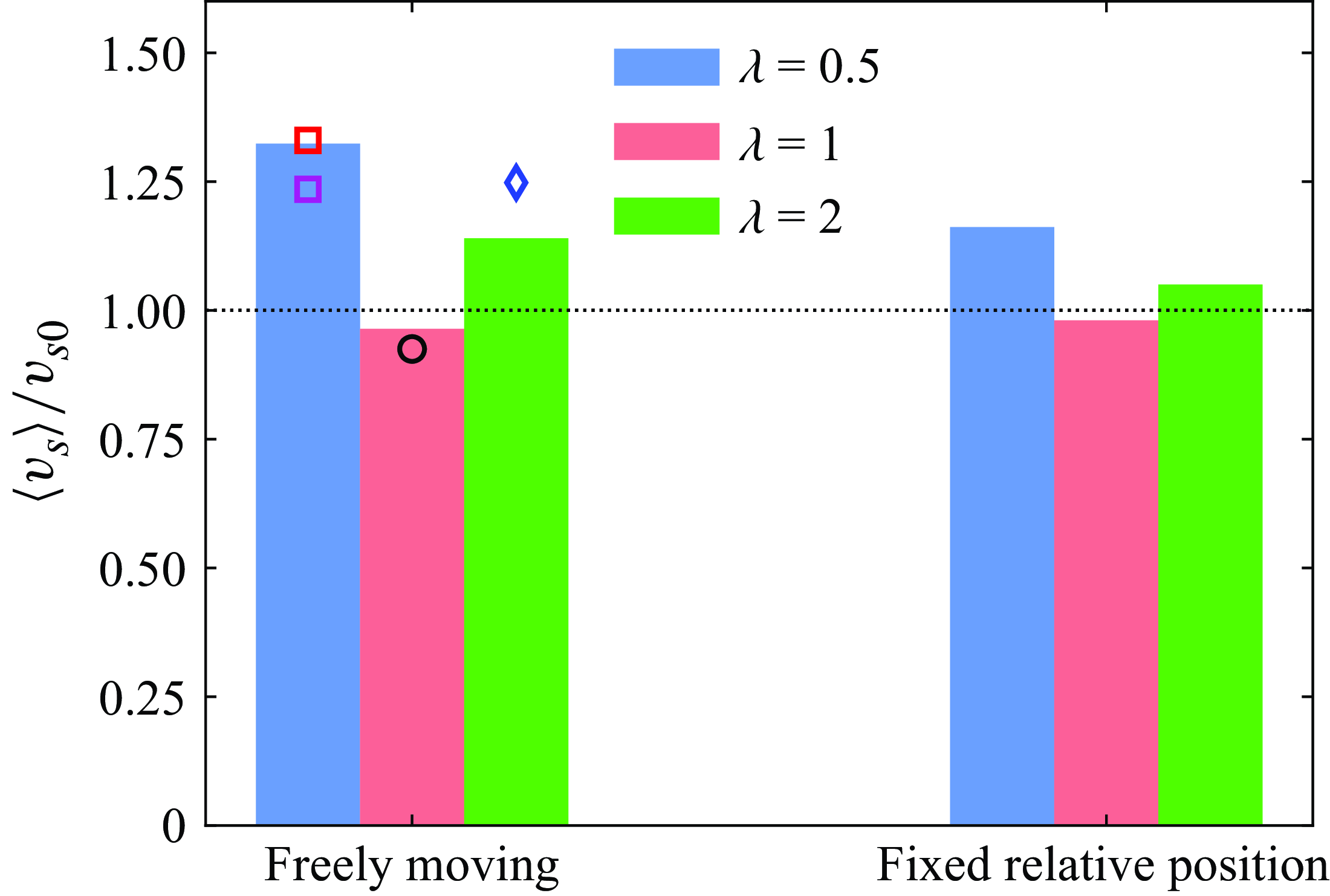
to represent the ensemble average over particles and time. In figure 2, we present the particle mean settling velocity normalized by the isolated-particle settling velocity in each case. In terms of the particle shape, the value of
 $\langle v_s \rangle /v_{s0}$
is greatest for oblate particles, and smallest for spherical particles, no matter whether the particles move freely or have fixed relative positions. In contrast to the decreased settling rate of spherical particles, the mean settling velocity is enhanced in the suspensions of spheroidal particles, which is in qualitative agreement with the reference data provided in figure 2. Comparing the results in the literature, we can see that the enhanced settling rate of spheroidal particles tends to increase with the non-sphericity of the particle shape. However, the degree of change in the settling velocity, measured by the ratio
 $\langle v_s \rangle /v_{s0}$
, is reduced in the fixed relative position (FRP) cases compared to freely moving (FM) particles. The slight reduction of the mean settling velocity for spherical particles can be ascribed to the effect of hindrance (Di Felice Reference Di Felice1999; Yin & Koch Reference Yin and Koch2007). For oblate and prolate spheroids, the settling motion is further modulated by the change of particle orientation and spatial distribution in the suspension. The influence of these two effects is elaborated in the following.
Mean settling velocity of the particles in suspensions in the present study (bars). Relevant results in the literature are also included for comparison (markers). Black circle: spherical particles with
 $\gamma =2$
,
 $Ga=70$
and
 $\phi =1\,\%$
(Seyed-Ahmadi & Wachs Reference Seyed-Ahmadi and Wachs2021). Red square: oblate particles with
 $\lambda =1/3$
,
 $\gamma =1.02$
,
 $Ga=60$
and
 $\phi =0.5\,\%$
(Fornari et al. Reference Fornari, Ardekani and Brandt2018). Magenta square: oblate particles with
 $\lambda =2/3$
,
 $\gamma =1.5$
,
 $Ga=110$
and
 $\phi =0.5\,\%$
(Moriche et al. Reference Moriche, Hettmann, García-Villalba and Uhlmann2023). Blue diamond: prolate particles with
 $\lambda =3$
,
 $\gamma =1.5$
,
 $Ga=80$
and
 $\phi =1\,\%$
(Jiang et al. Reference Jiang, Xu and Zhao2024b
).

3.2. Particle orientation
First, we examine the orientation of particles in the suspension. In figure 3, we report the statistical distribution of the particle pitch angle for the FM particles of different shapes. The results of the FRP cases are not shown since the probability density function of the particle orientation
 $\text{p.d.f.}(|{\cos \theta} |)\equiv 1$
for particles with initially random orientation that are not allowed to rotate. As shown in figure 3, FM oblate and prolate spheroids exhibit a preferential orientation with the major axis perpendicular to the gravitational direction, i.e.
 $|{\cos \theta} |=0$
for the prolate spheroid, and
 $|\cos \theta |=1$
for the oblate spheroid. This is the stable orientation of an isolated settling spheroid under the effect of fluid inertial torque (Dabade et al. Reference Dabade, Marath and Subramanian2015; Ardekani et al. Reference Ardekani, Costa, Breugem and Brandt2016), which has also been confirmed by our simulations of isolated settling oblate and prolate spheroids. The spherical particle is isotropic in shape, thus the value of
 $|\cos \theta |$
naturally conforms to a uniform distribution. Moreover, it is shown in figure 3 that the probability density function of the particle orientation (
 $\text{p.d.f.}(|{\cos \theta} |)$
) of oblate particles has a greater peak value and decays more rapidly near the peak value, than the p.d.f. of prolate spheroids. However, the tail of
 $\text{p.d.f.}(|{\cos \theta} |)$
is steeper for prolate particles than for oblate ones. These observations indicate the stronger intermittency in the orientation of oblate spheroids than prolate particles under the effect of the complex particle–fluid interactions. Oblate particles show a stronger tendency to keep the stable orientation, and are also more prone to orient with the broad side aligning to the gravitational direction (i.e.
 $|\cos \theta |=0$
), while the opposite is true for prolate particles.
The p.d.f. of the absolute value of the cosine of the particle pitch angle (see figure 1 for the definition of the particle pitch angle
 $\theta$
).

It is well known that the drag coefficient for a fixed spheroid in a uniform flow depends on the relative angle between the axis of the spheroid and the inflow direction (Zastawny et al. Reference Zastawny, Mallouppas, Zhao and van Wachem2012; Fröhlich et al. Reference Fröhlich, Meinke and Schröder2020). Hence the settling velocity of non-spherical particles can be modulated by the change of their orientation. We note that the isolated settling velocity
 $v_{s0}$
is measured for the spheroid with the broad-side-on orientation, which corresponds to the configuration with the maximum drag coefficient. Therefore, as for the spheroidal particles in the FRP cases, the randomization of the particle orientation increases the percentage of tilted particles, reducing the average drag coefficient experienced by the particles. Under this effect, the mean settling velocity should increase to balance the total gravitational forces of all particles. This mechanism, which overwhelms the weak hindrance effect (in view of the low volume fraction or our suspensions), results in the enhancement of the mean settling velocity (i.e.
 $\langle v_s \rangle \gt v_{s0}$
) observed for oblate and prolate particles in the FRP cases.
The joint probability density function (JPDF) (normalized by the maximum value) of the particle settling velocity and orientation. The solid lines represent the average of the settling velocity conditioned on
 $|\cos \theta |$
(denoted by
 $\langle v_s \rangle _\theta$
). The data are masked when
 $\text{p.d.f.}(|{\cos \theta} |)\lt 0.01 \max \{\text{p.d.f.}(|{\cos \theta} |)\}$
.

Regarding the cases of FM particles, we will examine the effect of particle orientation by studying the correlation between the settling velocity and the orientation of the dispersed particles. In figure 4, we depict the joint probability density function of
 $v_s$
and
 $|\cos \theta |$
for the different particle shapes under investigation. The data show that non-spherical particles tend to accelerate the settling motion as the orientation deviates more from the broad-side-on alignment, which is consistent with the reduced drag coefficient for the isolated spheroid as
 $\theta$
deviates from
 $\theta _0$
. Specifically, the conditionally averaged settling velocity, denoted by
 $\langle v_s \rangle _\theta$
, increases rapidly as
 $|\cos \theta |$
deviates from 1 for oblate spheroids, while the variation of
 $\langle v_s \rangle _\theta$
is moderate for prolate spheroids with the changing
 $|\cos \theta |$
. These trends are similar to that of the variation of
 $\text{p.d.f.}(|{\cos \theta} |)$
near
 $\theta _0$
displayed in figure 3. However, it is noteworthy from figure 2 that the mean settling velocity for FM spheroids is much larger than that for FRP particles, although the particle orientations in the latter cases are farther from the broad-side-on alignment (the maximum-drag orientation) than in the former cases. This indicates that the enhancement of the mean settling velocity for FM spheroidal particles cannot be solely ascribed to the change of orientation. In what follows, we therefore investigate the effect of the spatial distribution on the settling motion of the FM particles.
3.3. Particle clustering
3.3.1. Visualization of the flow and the particle pair correlation
Initially, we provide visualizations of the instantaneous three-dimensional flow fields together with the dispersed particles for the FM cases in figure 5. One can observe large-scale fluid structures in the suspensions with non-spherical particles, illustrated by the iso-surface of the vertical fluid velocity,
 $u_y=-v_{s0}$
. These flow structures, extending vertically across the whole computational domain, are the footprints of column-like particle clusters. The case with spherical particles, however, is characterized by the small-scale wakes of spheres settling almost in isolation, as shown in figure 5(b). In previous studies, researchers have linked the formation of particle clusters to the wake-induced hydrodynamic interactions among settling particles, which is the same mechanism behind the DKT process for a pair of settling particles (see, among others, Zaidi et al. Reference Zaidi, Tsuji and Tanaka2014; Fornari et al. Reference Fornari, Ardekani and Brandt2018). As for spherical particles, the absence of particle clusters in the current simulation is explained by the weak intensity of the particle wakes due to the relatively low settling Reynolds number (Zaidi et al. Reference Zaidi, Tsuji and Tanaka2014); the stronger wake-induced hydrodynamic interactions occurring for spheroidal particles (Ardekani et al. Reference Ardekani, Costa, Breugem and Brandt2016; Moriche et al. Reference Moriche, Hettmann, García-Villalba and Uhlmann2023) are responsible for the emergence of clustering in the suspensions of oblate/prolate particles observed in figure 5(a,c).
Snapshots of the vertical velocity of the fluid flow and particle distribution in the FM cases for (a) oblate particles, (b) spherical particles and (c) prolate particles. The iso-surfaces in red represent the vertical fluid velocity with
 $u_y=-v_{s0}$
. Particle surfaces are depicted in grey.

Pair correlation functions
 $P(r,\psi )$
from the simulations of FM particles for (a) oblate spheroids, (b) spherical particles and (c) prolate particles.

To better understand the micro-structure of the particles in the suspension, we examine the spatial correlation of the dispersed phase. Figure 6 illustrates the two-dimensional pair correlation function
 $P(r,\psi )$
(for the definition, see Yin & Koch Reference Yin and Koch2007; Fornari et al. Reference Fornari, Ardekani and Brandt2018), for the particles with different shapes. The function
 $P(r,\psi )$
estimates the probability of finding particle pairs with separation
 $(r_x,r_y)$
(or equivalently,
 $(r,\psi )$
in spherical coordinates), in which
 $r_x=r \cos \psi$
and
 $r_y=r \sin \psi$
represent the horizontal and vertical distances between two particles. The value of
 $P(r,\psi )$
is larger than 1 if the probability of finding a particle pair with separation
 $(r,\psi )$
is higher than for randomly distributed particles, whereas
 $P(r,\psi )\lt 1$
indicates regions depleted of particles.
As shown in figure 6(a,c), the value of
 $P(r,\psi )$
is greater than unity for close-by particles along the vertical direction, indicating vertical arrangements of settling oblate/prolate particles in the suspension. This observation is consistent with the column-like particle clusters displayed in figure 5(a,c). Moreover, the value of
 $P(r,\psi )$
decays slowly as the separation distance
 $r$
increases along the vertical direction, especially for oblate particles, which is in agreement with the finding of settling low-aspect-ratio oblate particles by Moriche et al. (Reference Moriche, Hettmann, García-Villalba and Uhlmann2023). These authors argue that the particle clusters can continuously grow to a size as large as the entire periodic computational domain, once the dispersed particles start to attract each other by DKT-like interactions. However, as shown in figure 6(b), the vertically aligned particle micro-structures are absent for non-clustering settling spheres. Instead, we observe a region devoid of particles at the separation distance
 $r \lesssim 2D_{eq}$
within the range of azimuthal angle
 $40^{\circ } \lesssim \psi \lesssim 70^{\circ }$
. This void region is also accompanied by a relatively high particle correlation along the horizontal direction, similar to the observations reported in Yin & Koch (Reference Yin and Koch2007) and Shajahan & Breugem (Reference Shajahan and Breugem2023). We attribute the presence of the void region to the rapid tumbling and separation of particle pairs during the DKT-like events. After that, particle pairs separate and form horizontally aligned pairs that enhance the particle correlation in the horizontal direction (Yin & Koch Reference Yin and Koch2007).
3.3.2. Voronoi analysis
Next, we conduct a Voronoi analysis to quantify the clustering of the dispersed particles (Monchaux et al. Reference Monchaux, Bourgoin and Cartellier2010). We report the p.d.f. of the normalized Voronoi volumes in figure 7(a) for the FM cases with different particle shapes. It is observed that the probability of finding Voronoi tessellations with small and large volumes is significantly higher for non-spherical particles, especially for oblate spheroids, than for spherical particles. This indicates an increased percentage of volumes with close-by particles, as well as voids, in suspensions of non-spherical particles, which is a sign of particle clustering (Monchaux et al. Reference Monchaux, Bourgoin and Cartellier2010). The clustering indicator
 $C$
(see (2.19) for its definition) shown in figure 7(b) also confirms the morphology of clustering for non-spherical particles (
 $C\gt 1$
). In particular, in the suspension of oblate particles, the standard deviation of the normalized Voronoi volume is greater than that of a random distribution by more than
 $90\,\%$
. The significant clustering of oblate particles can be related to the stable piled-up configuration of pairwise oblate spheroids during the DKT process (Ardekani et al. Reference Ardekani, Costa, Breugem and Brandt2016; Fornari et al. Reference Fornari, Ardekani and Brandt2018). In contrast, the p.d.f. of
 $\overline {V}_{Voro}$
is narrow, and the value of
 $C$
is lower than unity for spherical particles. The deviation from the random spatial distribution for spherical particles is related to the horizontally aligned particle micro-structures observed in figure 6(b).
Voronoi analysis of the spatial distribution of FM particles. (a) The p.d.f. of the normalized Voronoi volumes. The dotted line illustrates the p.d.f. associated with a random distribution of spherical particles for comparison. (b) Clustering indicator for particles with different shapes.

The joint probability density function (JPDF) of the particle settling velocity and the normalized Voronoi volume in the FM cases with (a) oblate particles, (b) spherical particles and (c) prolate particles. The solid lines represent the average settling velocity conditioned on the normalized Voronoi volume (the data are masked when
 $\text{p.d.f.}(\overline {V}_{Voro})\lt 0.001\max ({\text{p.d.f.}(\overline {V}_{Voro})})$
).

To gain further insights, we investigate the correlation between the particle settling motion and the particle clustering. We therefore illustrate the joint probability density function of the settling velocity and Voronoi volume for the FM particles of different shapes in figure 8. Interestingly, in the cases with significant particle clustering (oblate/prolate particles; see figure 8
a,c), we can observe an evident negative correlation between
 $v_s$
and
 $\overline {V}_{Voro}$
. In other words, particles tend to settle faster in the regions where the local concentration is higher, and vice versa. This can be interpreted by the preferential sampling of downward wake flows by the locally accumulated particles (corresponding to small values of
 $\bar {V}_{Voro}$
) (Uhlmann & Doychev Reference Uhlmann and Doychev2014; Jiang et al. Reference Jiang, Xu and Zhao2024b
). As a consequence, a cluster of particles experiences a smaller total hydrodynamic drag than the sum of the drag of the same number of isolated particles (Koch & Hill Reference Koch and Hill2001; Dodds et al. Reference Dodds, Sarhan and Naser2020). On the contrary, in the regions depleted of particles (i.e. for large values of
 $\bar {V}_{Voro}$
), the settling velocity is reduced to less than that of an isolated particle due to the effect of hindrance (Di Felice Reference Di Felice1999). However, for spherical particles, the correlation between
 $v_s$
and
 $\overline {V}_{Voro}$
becomes less pronounced (see figure 8
b), which can be attributed to the orderly arrangement of settling spheres in space. According to the above discussion, it is not surprising that the mean settling velocity of the dispersed particles is highly correlated to the degree of particle clustering, which can be identified by comparing figure 2 with figure 7(b). Similar findings were also reported in the studies by Uhlmann & Doychev (Reference Uhlmann and Doychev2014) and Moriche et al. (Reference Moriche, Hettmann, García-Villalba and Uhlmann2023) about the sedimentation of particles with different Galileo numbers and shapes.
3.3.3. Size of particle clusters
To deepen the analysis, we also estimate the sizes of clusters in the FM cases with different particle shapes. Specifically, we regard two particles as part of the same cluster if their centre-to-centre distance, denoted by
 $d_{cc}$
, satisfies
 $d_{cc}\lt 0.5\phi ^{-1/3}D_{eq}$
. The factor
 $\phi ^{-1/3}$
is included in the definition to consider the effect of volume fraction, as the mean distance between two neighbouring particles decays with
 $\phi ^{-1/3}$
in a particle assembly. We define the size of particle clusters by the number of member particles
 $N$
, with
 $N=1$
indicating an isolated particle (see, among others, Fornari et al. Reference Fornari, Ardekani and Brandt2018). In figure 9, we present the fraction of the total particle number (denoted by
 $\chi$
) and the averaged settling velocity (denoted by
 $\langle v_s \rangle _N$
) in clusters with different sizes. As shown in figure 9(a), oblate particles are most prone to form large-size clusters, with more than
 $30\,\%$
of the particles being found in clusters with
 $N\geqslant 10$
. In contrast, the percentage of isolated spherical particles (
 $N=1$
) is considerably higher than that of non-spherical particles, and clusters with
 $N\gt 5$
are very seldom found for settling spheres. Regarding the settling velocity, it is indicated by figure 9(b) that the non-spherical particles pertaining to the clusters with the larger size tend to settle more rapidly; however,
 $\langle v_s \rangle _N$
becomes almost independent of the cluster size for spherical particles. These observations are in qualitative agreement with the results shown in figure 8 on the Voronoi analysis, and further confirm the significance of clustering on the particle settling velocity in the suspension.
(a) The fraction of the total number of particles forming clusters with
 $N$
particles. (b) The averaged settling velocity of the particles within clusters of different sizes.

4. Particle-induced turbulence
In this section, we will examine the pseudo-turbulence induced by the settling particles, following the denomination used for turbulence induced by rising bubbles, to which we will compare the present results.
4.1. One-point statistics of the fluid velocity fluctuations
We start with the one-point statistics of the fluid velocity fluctuations in the particle-induced turbulent flows. Here, the fluid velocity fluctuation is defined by
 $u_i'=u_i-\langle u_i \rangle _f$
, in which
 $\langle {\boldsymbol\cdot} \rangle _f$
denotes the average within the domain occupied by the fluid phase. For the present flow system, the two horizontal velocity components (along the
 $x$
and
 $z$
directions) are statistically equivalent with zero mean velocity (i.e.
 $\langle u \rangle _f=\langle w \rangle _f=0$
), while there is a mean upward flow along the vertical direction, with
 $\langle v \rangle _f=\phi \langle v_s \rangle /(1-\phi )$
to maintain the zero flux of the whole system (Yin & Koch Reference Yin and Koch2007). In figure 10, we present p.d.f.s of the fluctuations of the horizontal and vertical fluid velocities for each case under consideration. It is shown that the horizontal velocity fluctuation exhibits a symmetric distribution, while the p.d.f. of
 $v'$
is skewed with a slow decay for the negative tail. This observation is the result of downward wake flow behind settling particles, resembling the statistical distribution of the velocity fluctuations in bubble-induced pseudo-turbulence (Riboux et al. Reference Riboux, Risso and Legendre2010). Considering the cases with FRP particles, the shape effect on the p.d.f.s is marginal. The horizontal velocity fluctuation is highly localized around
 $u'=0$
, with a pronounced peak. On the other hand, the p.d.f. of
 $v'$
exhibits a secondary peak at
 $v'\approx -v_{s0}$
, which can be interpreted by the identical settling velocity for all the dispersed particles in this scenario.
Probability density functions of the fluctuations of (a,b) the horizontal fluid velocity, and (c,d) the vertical fluid velocity: (a,c) simulations of FRP particles; (b,d) simulations of FM particles.

In contrast, the statistical distribution of the fluid velocity fluctuation exhibits greater shape dependency in the cases with FM particles. The p.d.f.s of
 $u'$
and
 $v'$
for spherical particles are similar to those of the FRP case, but they are significantly broader, with a longer negative tail in the cases with oblate and prolate particles (see figure 10
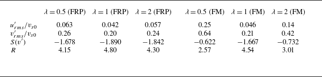
c,d). These observations are quantified by the root mean square and the skewness of the velocity fluctuations provided in table 2. As a matter of fact, the oblate/prolate particles exhibit stronger horizontal motions than spherical particles (not shown here) because of the lateral drift of settling spheroids with inclined orientations (Jiang et al. Reference Jiang, Xu and Zhao2024c
). This mechanism results in enhanced fluctuations of the horizontal fluid velocity in the corresponding cases. Moreover, the fluid flows in the regions surrounded with particle clusters (dominated by downward wake flows) and voids (dominated by upward mean flows) contribute differently to the vertical fluid velocity, giving rise to the enhanced vertical velocity fluctuations for the cases with non-spherical particles, in particular oblate particles when clustering is most prominent. In addition, although the prevalence of particle clusters intensifies the downward fluid flow (with the increased probability to observe negative
 $v'$
of large magnitude), the disappearance of the local peak of the p.d.f. at
 $v'\approx -v_{s0}$
explains the reduced skewness
 $S(v')$
in the cases with FM oblate/prolate particles.
Quantification of the fluid velocity fluctuations. The subscript
 $rms$
here represents the root mean square. The skewness of the vertical velocity fluctuation is denoted by
 $S(v')$
. The ratio
 $R=v'_{rms}/u'_{rms}$
is used to measure the flow anisotropy.

In table 2 we also report the ratio between the root mean square values of the vertical and horizontal velocity fluctuations. We use this quantity to measure the anisotropy of the current fluid flows. Basically, the results show that the value of
 $v'_{rms}/u'_{rms}$
is always greater than unity, indicating stronger fluctuations in the vertical velocity component. However, it is interesting to note a significantly lower flow anisotropy in the cases with FM oblate/prolate particles compared with other cases. We will discuss the correlation between this observation with the particle clustering in § 4.2.2.
4.2. Energy spectra and scale-by-scale budget of the particle-induced turbulence
4.2.1. Total energy analysis
In what follows, we perform a spectral analysis of the pseudo-turbulence induced by settling particles. Referring to the derivation in § 2.4.2, we obtain the scale-by-scale budget of the turbulence kinetic energy (TKE) in spectral space by taking the summation over index
 $i$
in (2.23):
 \begin{equation} \frac {\partial \mathcal{E}_{k}\left (\boldsymbol{\kappa }\right )}{\partial t}=\mathcal{T}_{k}\left (\boldsymbol{\kappa }\right )+\mathcal{P}_{k}\left (\boldsymbol{\kappa }\right )+\mathcal{D}_{k}\left (\boldsymbol{\kappa }\right )+\mathcal{F}_{k}\left (\boldsymbol{\kappa }\right ). \end{equation}
Here, the subscript
 $k$
represents the TKE, and a generic term
 $\mathcal{J}_k(\boldsymbol{\kappa })$
in (4.1) is defined as
 $\mathcal{J}_k(\boldsymbol{\kappa })=\sum \limits _{i=1,2,3}{\mathcal{J}_i(\boldsymbol{\kappa })}$
, where
 $\mathcal{J}$
could be
 $\mathcal{E}$
,
 $\mathcal{T}$
,
 $\mathcal{P}$
,
 $\mathcal{D}$
or
 $\mathcal{F}$
. Accordingly, the TKE is the summation of
 $\mathcal{E}(\boldsymbol{\kappa })$
over all wavenumbers, i.e.
 \begin{equation} k = \frac {1}{2}\left \langle {u^2 + v^2 + w^2} \right \rangle = \sum \limits _{\boldsymbol{\kappa }} {\mathcal{E}_k ({\boldsymbol{\kappa }})}. \end{equation}
Similarly, the total dissipation rate can be related to
 $\mathcal{D}(\boldsymbol{\kappa })$
by
 \begin{equation} \varepsilon = - 2 \nu \langle s_{ij} s_{ij} \rangle = \sum \limits _{\boldsymbol{\kappa }} {\mathcal{D}_k ({\boldsymbol{\kappa }})}, \end{equation}
where
 $s_{ij}$
denotes the tensor of the velocity deformation rate. The term
 $\mathcal{F}_k$
in (4.1) represents the work associated with the IB forces, which reflects the particle–fluid interactions. Note that the gravitational potential energy of the settling particles is injected into the fluid flow via IB forces. Hence
 $\mathcal{F}_k$
serves as the energy production of the fluid flow, and we have the relationship
 $\sum_{\boldsymbol{\kappa }} {\mathcal{F}_k ({\boldsymbol{\kappa }})}=-\varepsilon$
in the steady state. As we will show below, the work done by IB forces inputs energy in the fluid flow over a broad range of scales, not only at the largest ones as in the classic homogeneous isotropic turbulence. Also, this energy production varies among the different cases, and is related to the different flow and particle structures in the current system.
Energy spectra versus the wave vector magnitude for all cases under consideration: (a) FRP particles, (b) FM particles. The dotted vertical line represents the wavenumber corresponding to the particle equivalent diameter, i.e.
 $\kappa _D=2{\unicode{x03C0}} /D_{eq}$
.

To begin with, we report in figure 11 the spherical shell integral of the energy spectra, i.e. the energy as a function of the wave vector magnitude
 $\kappa = \| \boldsymbol{\kappa } \|$
, for all cases under consideration. First, we observe in figure 11(a) that the energy spectra, normalized by the TKE, almost collapse for all the FRP cases, despite the different particle shapes. The only difference is that the oscillation of the energy spectra at
 $\kappa \gtrsim \kappa _D$
is more severe for settling spheres. This kind of oscillation is caused by the presence of dispersed particles in the fluid due to the so-called ‘boxcar effect’ (Lucci et al. Reference Lucci, Ferrante and Elghobashi2010). According to the quantitative analysis by Lucci et al. (Reference Lucci, Ferrante and Elghobashi2010) and Ramirez et al. (Reference Ramirez, Burlot, Zamansky, Bois and Risso2024), the period of the oscillation
 $T_{osci}=2{\unicode{x03C0}} /D$
corresponds to the diameter of spherical particles. Our results in figure 11 are in agreement with this theory. Additionally, the oscillations of the energy spectra are damped for the cases with spheroidal particles, since oscillation periods varying between
 $2{\unicode{x03C0}} /D_{max}$
and
 $2{\unicode{x03C0}} /D_{min}$
(where
 $D_{min}$
and
 $D_{max}$
represent the minor and major axes of the spheroid) cancel each other out (Ramirez et al. Reference Ramirez, Burlot, Zamansky, Bois and Risso2024). Similar oscillations were also reported in the energy spectra of particle-laden homogeneous isotropic turbulence, and have negligible effect on the physical interpretation of the results (Wang et al. Reference Wang, Ayala, Gao, Andersen and Mathews2014; Chiarini & Rosti Reference Chiarini and Rosti2024). For the cases with FM particles, however, figure 11(b) demonstrates that more energy is contained at large scales for the flows with oblate/prolate spheroids than for spherical particles. This observation is related to the large-scale flow structures accompanied by the large-scale particle clusters shown in figure 5. Moreover, we can clearly observe a
 $\kappa ^{-3}$
decay for the energy spectra at scales comparable to or smaller than the particle size, regardless of the particle shape and motion type (FM or FRP). This power law of the energy spectra has been widely reported in previous studies on bubble-induced pseudo-turbulence (Lance & Bataille Reference Lance and Bataille1991; Riboux et al. Reference Riboux, Risso and Legendre2010; Roghair et al. Reference Roghair, Mercado, van Sint Annaland, Kuipers, Sun and Lohse2011; Risso Reference Risso2011). In Lance & Bataille (Reference Lance and Bataille1991), the
 $\kappa ^{-3}$
power law of the energy spectra was originally explained by the assumption of a local balance between the energy production (estimated by
 $\kappa ^{-1} \varepsilon _w$
, where
 $\varepsilon _w$
is the viscous dissipation in the wake) and the dissipation (
 $ \mathcal{D}(\kappa )=-2\textit{v} \kappa ^2\, \mathcal{E}(\kappa )$
) on the corresponding scales. Note, however, that a similar power law was also observed for bubble-induced turbulence in Pandey et al. (Reference Pandey, Ramadugu and Perlekar2020) and Zamansky et al. (Reference Zamansky, Le Roy De Bonneville and Risso2024), where the viscous dissipation is seen to balance both nonlinear transfer and turbulence production by the interphase coupling.
Spherical integral of the budget terms (each term is normalized by
 $\varepsilon D_{eq}$
) of the TKE for: (a) oblate particles, (b) spherical particles and (c) prolate particles. The solid lines represent the FM cases, while the dashed lines correspond to the FRP cases. The inset in (a) depicts a zoomed-in view of the data in the same figure with a reduced range of the vertical axis. The dotted vertical line in each plot represents the wavenumber
 $\kappa =\kappa _D$
.

To examine the aforementioned assumption in the current configurations, we further investigate the energy budget in the particle-induced turbulent flows. To this end, we compute the scale-by-scale budgets of the TKE, and report the contribution from each term on the right-hand side of (4.1) in figure 12. Note that the term related to pressure,
 $\mathcal{P}_k$
, vanishes because of the incompressible constraint of the flow. As a feature common to all cases, the energy transfer by the nonlinear terms,
 $\mathcal{T}_k$
, is acting primarily on scales larger than the particle size. At smaller scales with
 $\kappa \gtrsim \kappa _D$
, the contribution of
 $\mathcal{T}_k$
decays faster than
 $\mathcal{F}_k$
and
 $\mathcal{D}_k$
. Within this range of wavenumbers, the work done by the IB forces approximately balances the viscous dissipation, i.e.
 $\mathcal{F}_k(\kappa ) \approx -\mathcal{D}_k(\kappa )$
. Our results show therefore that the idea proposed by Lance & Bataille (Reference Lance and Bataille1991) regarding the local balance between interphase energy transfer and viscous dissipation applies also to the case of particle sedimentation. Note, however, that unlike the case of deformable bubbles where dissipation is found in the wakes, viscous dissipation in suspensions of settling rigid spheres is expected to occur in the near-boundary regions on the front and lateral sides of the particles; see figure 8 in Fornari et al. (Reference Fornari, Picano and Brandt2016). By virtue of the dimensional analysis, the energy input by the IB forces can be estimated by
 $\mathcal{F}_k \sim \kappa ^{-1} \varepsilon _{sl}$
(with
 $\varepsilon _{sl}$
representing the viscous dissipation in the shear layer near the particle surfaces) on these small scales, since the energy injection by gravity contributes mainly to the energy budget on the scales larger than the dispersed phase (Pandey et al. Reference Pandey, Ramadugu and Perlekar2020; Ramirez et al. Reference Ramirez, Burlot, Zamansky, Bois and Risso2024). As a consequence, we arrive at the
 $\kappa ^{-3}$
scaling law of the energy spectra by considering the balance
 $\mathcal{F}_k(\kappa ) \approx -\mathcal{D}_k(\kappa )$
. Additionally, a similar local balance for the flow budget was also reported in homogeneous shear turbulence laden with sub-Kolmogorov particles (Gualtieri et al. Reference Gualtieri, Picano, Sardina and Casciola2013, Reference Gualtieri, Battista and Casciola2017). However, the local energy input due to the feedback from the tiny particles was shown to scale with
 $\kappa ^{-2}$
at scales
 $\kappa \eta \approx 1$
(with
 $\eta$
being the Kolmogorov length scale), leading to a
 $\kappa ^{-4}$
power law of the energy spectrum (Gualtieri et al. Reference Gualtieri, Battista and Casciola2017), whereas in the numerical model by Le Roy De Bonneville et al. (Reference Le Roy De Bonneville, Zamansky, Risso, Boulin and Haquet2021) and Zamansky et al. (Reference Zamansky, Le Roy De Bonneville and Risso2024), although the interface is not resolved, interactions between bubble wakes are. This leads to the
 $\kappa ^{-3}$
scaling of the energy spectra, similar to the case of large bubbles or particles. These authors attributed this scaling to the mean shear rate imposed by the bubbles, which controls the rate of return to isotropy. We therefore conjecture that two-way coupling approaches not modelling wake interactions can be relevant only at low volume fractions or for very small particles.
Let us now move to the large scales where the energy injection due to gravity dominates. It is noteworthy from figure 12 that the work done by the IB forces,
 $\mathcal{F}_k$
, exhibits a striking peak at the smallest wavenumber in the cases of FM spheroidal particles. As discussed in § 3.3, settling oblate or prolate particles tend to form column-like clusters whose scale could become comparable to the entire computational domain (Moriche et al. Reference Moriche, Hettmann, García-Villalba and Uhlmann2023). Consequently, energy is injected into the flow primarily by the interaction between the fluid flow and these large-scale particle clusters. This mechanism is also responsible for the rise of energy spectra
 $\mathcal{E}_k$
at small wavenumbers in the FM cases with oblate/prolate particles (see figure 11
b), corresponding to the large-scale flow structures displayed in figure 5(a,c). Moreover, we also notice that the magnitude of the peak value of
 $\mathcal{F}_k$
on a large scale is correlated to the degree of particle clustering, and vanishes when the particle clustering is absent or not allowed.
Distribution of the energy spectra in cylindrical coordinates (
 $\mathcal{E}_k^C$
) in the spectral space for (a–c) the FRP cases and (d–f) the FM cases, for (a,d) oblate particles, (b,e) spherical particles and (c,f) prolate particles. The red lines highlight the wavenumbers corresponding to the particle size, i.e.
 $\kappa _r=\kappa _D$
and
 $\kappa _v=\kappa _D$
.

Distribution of the work done by the IB force in cylindrical coordinates (
 $\mathcal{F}_k^C$
) in the spectral space for (a–c) the FRP cases and (d–f) the FM cases, for (a,d) oblate particles, (b,e) spherical particles and (c,f) prolate particles. For clarity, we display only the results at large scales with
 $\kappa _r \leqslant \kappa _D$
and
 $\kappa _v \leqslant \kappa _D$
. The red triangle in (d,f) corresponds to the wavenumber
 $(\kappa _r,\kappa _v)=(2{\unicode{x03C0}} /L_x,0)$
.

To gain further understanding about the characteristics of the particle-induced pseudo-turbulence, we now examine the spectra of TKE and its budget in cylindrical coordinates in spectral space, as introduced in § 2.4.2. First, we depict the two-dimensional maps of
 $\mathcal{E}_k^C$
in the
 $\kappa _r{-}\kappa _v$
plane in figure 13 (refer to (2.25) for its definition). Compared to the spherical integral of the energy spectra presented in figure 11, the energy density represented by
 $\mathcal{E}_k^C$
additionally provides directional information for the distribution of TKE in the spectral space. We will note that for the single-phase homogeneous isotropic turbulence, the isotropic distribution of energy yields contour lines of
 $\mathcal{E}_k^C$
that are symmetric about the diagonal line in the
 $\log \kappa _r{-}{\log \kappa _v}$
plane (not shown here). For the particle-induced pseudo-turbulence, instead, we observe in figure 13 that the energy spectra decay more rapidly along the vertical than the horizontal direction. This kind of anisotropy is mainly exhibited at scales larger than the particle size, seemingly due to the flow structures induced by the particle settling motion. In the horizontal direction, thin shear layers exist besides the downward-moving particles, which are reflected by the energy at high horizontal wavenumber
 $\kappa _r$
. In contrast, the flow structures are elongated in the vertical direction (including the particle wakes or the streaks of upcoming fluid on their side), corresponding to more energy at low vertical wavenumbers
 $\kappa _v$
. Interestingly, this anisotropy is less prominent for the flows induced by FM non-spherical particles, although the column-like particle clusters are longer in these cases. This will be discussed further when commenting on figure 15 about the role of the nonlinear energy transfer among scales. Finally, at small scales (great values of
 $\kappa _r$
and
 $\kappa _v$
), the energy spectra
 $\mathcal{E}_k^C$
progressively recover isotropy.
In figures 14–16, we illustrate the scale-by-scale budget terms of TKE (except for the vanishing term
 $\mathcal{P}_k^C$
) in cylindrical coordinates (visualized on the
 $\kappa _r{-}\kappa _v$
plane). Incidentally, we display only the data with low wavenumbers, i.e.
 $\kappa _r\lt \kappa _D$
and
 $\kappa _v\lt \kappa _D$
, since the budget terms decay rapidly and recover the isotropic distribution on small scales. Considering first the term
 $\mathcal{F}_k^C$
, the results shown in figure 14 indicate that the IB forces do work and inject energy at large scales in the vertical direction (low wavenumbers
 $\kappa _v$
); moreover, we observe that positive values of
 $\mathcal{F}_k^C$
cover a wider range of scales in the horizontal direction. Notably, in the cases of FM non-spherical particles, a striking peak of
 $\mathcal{F}_k^C$
is observed at the smallest values of
 $\kappa _v$
, which may be related to the particle clusters extending across the whole computational domain in the periodic vertical direction with a lateral span comparable to the horizontal domain size (Moriche et al. Reference Moriche, Hettmann, García-Villalba and Uhlmann2023). As a consequence, the peak value of
 $\mathcal{F}_k^C$
corresponds to the wavenumbers
 $\kappa _v=0$
and
 $\kappa _r=2{\unicode{x03C0}} /L_x$
in the FM cases of oblate/prolate particles, and is less sharp along the horizontal direction than the vertical direction. For the cases where particle clustering is absent, the aforementioned peak becomes less pronounced.
Same as figure 14, but for the nonlinear transfer spectra
 $\mathcal{T}_k^C$
.

Same as figure 14, but for the viscous dissipation spectra
 $\mathcal{D}_k^C$
.

Next, the effect of the nonlinear transfer is illustrated in figure 15. It is demonstrated that the energy is transferred by the nonlinear interactions not only between different radial scales (quantified by the term
 $\mathcal{T}_k(\kappa )$
in figure 12), but also in a more complex way along the azimuthal direction on the
 $\kappa _r{-}\kappa _v$
plane. Overall, we notice that the energy input by the fluid–particle interaction forces (corresponding to the peak value of
 $\mathcal{F}_k^C$
shown in figure 14) is efficiently transferred to the close regions near the
 $\kappa _v$
axis (which is most clear by the positive peak of
 $\mathcal{T}_k^C$
in figure 15
d). This process appears to be more significant in the suspensions of FM spheroidal particles. As a result, the anisotropic distribution of turbulence kinetic energy on the
 $\kappa _r{-}\kappa _v$
plane is more clearly mitigated for the flow of settling oblate/prolate particles than for the spherical ones (see figure 13), although the energy input exhibits stronger anisotropy in the non-spherical cases, as displayed in figure 14. We conjecture that this more efficient transfer in the presence of clustering might be due to the meandering of the particle-depleted regions and to the stronger wake–wake interactions in the clustering regions.
Finally, it is shown in figure 16 that the viscous dissipation
 $\mathcal{D}_k^C$
is also anisotropic, with larger energy dissipation at higher horizontal wavenumber
 $\kappa _r$
, corresponding to the thin shear layers in the wakes and beside the particle clusters. This is consistent with the anisotropic distribution of
 $\mathcal{E}_k^C$
presented in figure 13, considering the relationship
 $\mathcal{D}_k^C= -2\nu \kappa ^2 \mathcal{E}_k^C$
.
Budget terms of (a–c) the vertical component and (d–f) the horizontal component of TKE, for (a,d) oblate particles, (b,e) spherical particles and (c,f) prolate particles. The solid lines represent the FM cases, while the dashed lines represent the FRP cases.

4.2.2. Kinetic energies of the horizontal and vertical velocity components
As discussed in § 4.1, the particle-induced turbulence is anisotropic with stronger velocity fluctuations in the vertical direction. Therefore, in this subsubsection, we separately investigate the budgets of the fluctuation intensity for the vertical and horizontal components. To this end, we decompose the TKE
 $k$
into the vertical component
 $k_v=\langle v^2 \rangle /2$
and the horizontal component
 $k_h=\langle u^2 + w^2 \rangle/2$
, i.e.
 $k=k_v+k_h$
. Accordingly, the budgets of these vertical energy
 $k_v$
and horizontal energy
 $k_h$
are defined by
 $\mathcal{J}_v=\mathcal{J}_2$
and
 $\mathcal{J}_h=\mathcal{J}_1+\mathcal{J}_3$
, where
 $\mathcal{J}$
represents the arbitrary term
 $\mathcal{T}$
,
 $\mathcal{P}$
,
 $\mathcal{D}$
or
 $\mathcal{F}$
.
First, we illustrate the budget of the vertical component of the kinetic energy in figure 17(a–c). By comparing with figure 12, we find that the different contributions to the vertical turbulence kinetic energy are similar to those of the TKE (except for the non-zero pressure term
 $\mathcal{P}_v$
). This observation is explained by the predominance of the vertical fluid velocity in the pseudo-turbulent flow induced by the settling particles. It is also shown in figure 17(a–c) that the IB forces do positive work in the vertical direction as the source of the vertical kinetic energy. However, examining the budget for the horizontal component shown in figure 17(d–f), it is interesting to note that the pressure term
 $\mathcal{P}_h$
becomes positive and serves as the source of the horizontal kinetic energy. In contrast, the IB forces, which only transfer energy among different scales, have zero net contribution to the horizontal kinetic energy, namely
 $\sum \nolimits _{\boldsymbol{\kappa }} {\mathcal{F}_h ({\boldsymbol{\kappa }})}=0$
, similar to the turbulence modulation by finite-sized particles (Chiarini & Rosti Reference Chiarini and Rosti2024). In other words, due to the flow incompressibility, the pressure effectively redistributes part of the energy from the vertical component (as confirmed by the negative value of
 $\mathcal{P}_v$
in figure 17
a–c), and thus sustains the horizontal flow energy in this system. It is also noteworthy from figure 17(d,f) that the contribution from
 $\mathcal{P}_h$
is substantially augmented in the FM cases of oblate/prolate particles at large scales. Recalling the significant particle clustering in these cases, we speculate that the enhanced energy redistribution is related to the flow characteristics in the clustering regions. Finally, as a consequence of this redistribution by pressure forces, the unevenly allocated velocity fluctuations of the particle-induced pseudo-turbulence (the anisotropy feature; see table 2) is attenuated when the particle clustering is significant.
Finally, we wish to summarize the whole path of the energy transfer in the pseudo-turbulence induced by settling particles. Because of the settling motion of particles, fluid–particle interaction forces do positive work along the vertical direction, which is the source of energy in the whole flow system. A part of input energy is redistributed from the vertical velocity component to the horizontal components under the action of pressure, which sustains the horizontal velocity fluctuations. The energy is injected into the fluid flow by the settling motion of particles typically on scales larger than the particle size, and then is transferred among different scales by both nonlinear effects and the IB forces. At scales smaller than the particle size, however, viscous dissipation locally balances the work done by fluid–particle interaction forces, leading to the
 $\kappa ^{-3}$
power law of the energy spectra. The influence of particle clustering on the particle-induced turbulent flows is twofold. On the one hand, column-like particle clusters inject energy at larger scales, giving rise to the emergence of large-scale flow structures. On the other hand, the particle clustering also enhances the energy redistribution by pressure between the vertical and horizontal velocity components, by which the anisotropy of the particle-induced turbulence is attenuated.
5. Conclusions
In the present work, we studied the settling of spheroidal particles with different shape in an initially quiescent fluid by means of PR-DNS. We considered spheroids with aspect ratio
 $\lambda =0.5$
(oblate spheroids),
 $\lambda =1$
(spheres) and
 $\lambda =2$
(prolate spheroids). Under the current parameter set-ups, the isolate spheroid settles vertically without the wake and path instability. However, in the suspension, the dynamics of the settling particles and the fluid flow induced by the particle motion are significantly altered by complicated fluid–particle hydrodynamic interactions. To disentangle these, we performed simulations of freely moving (FM) particles and of an ideal suspension in which the particle relative position is fixed and the orientation is random.
We first examined the collective behaviour of the dispersed phase. It was found that the mean settling velocity is enhanced for oblate/prolate spheroids in the dilute suspension with solid volume fraction
 $\phi =1\,\%$
. On the one hand, the change of particle orientation, which is caused by the complicated particle–fluid and particle–particle interactions in the suspension, makes a contribution to accelerating the settling motion of spheroidal particles, deviating their orientation from the stable broad-side-on alignment. On the other hand, the spheroidal particles were found to form column-like clusters under the effect of the wake-induced hydrodynamic interactions. The settling motion of clustered particles can be enhanced substantially due to the preferential sampling of downward flow, which was confirmed by the correlation between the Voronoi volume (or the cluster size) and the settling velocity of non-spherical particles. Under this effect, the mean settling velocity is enhanced to the maximum degree for the FM oblate particles owing to the most significant particle clustering in that case. By contrast, the mean settling velocity is slightly reduced for spherical particles due to the hindrance effect, since the clustering is not present, and the effect of orientation is irrelevant to settling spheres.
Then we carefully investigated the fluid flow induced by settling particles. Although the wake of an isolated settling particle is steady, the instability induced by wake–wake interactions causes a spatiotemporal evolving flow, i.e. so-called particle-induced pseudo-turbulence. The one-point statistics of the fluid velocity indicate that the pseudo-turbulence is anisotropic, with higher fluctuations of the vertical than horizontal velocity, and the p.d.f.s of the fluid velocity fluctuations are non-Gaussian, similar to the observations in the bubble-induced pseudo-turbulence (Riboux et al. Reference Riboux, Risso and Legendre2010; Amoura et al. Reference Amoura, Besnaci, Risso and Roig2017). Moreover, we also identified a robust
 $\kappa ^{-3}$
power law of the energy spectra in the particle-induced turbulence at scales close to and smaller than the particle size. By further performing the scale-by-scale analysis of the energy budget, this power law of the energy spectra is explained by the local balance between the energy production from the fluid–particle interactions and dissipation (Lance & Bataille Reference Lance and Bataille1991).
In addition, we study the directional information of the energy spectra and budget in spectral space. We demonstrate that the anisotropy of the particle-induced turbulent flow is not only manifested by the unequal distribution of the turbulence kinetic energy in the horizontal and vertical velocity components, but also reflected by the anisotropic energy spectra and corresponding budgets in spectral space. The energy spectra are found to decay more rapidly along the vertical direction than the horizontal ones in cylindrical coordinates in spectral space, indicating the smaller scale of the typical horizontal flow structures (i.e. thin shear layers) compared with the longer vertical structures (i.e. wakes or flow streaks). Interestingly, this kind of anisotropic cascade of the energy spectra is less pronounced for the cases with significant particle clustering (i.e. FM oblate or prolate particles), although energy production by the fluid–particle interactions exhibits a higher degree of anistropy in these cases. This is linked to the intensified inter-scale energy transfer by the nonlinear effect when particle clustering is present, which is presumably related to meandering of regions depleted of particles and to the wake–wake interactions. Note that the return to isotropy has been correlated to the local shear in the wakes of rising bubbles (Zamansky et al. Reference Zamansky, Le Roy De Bonneville and Risso2024). Our results seem to confirm that the higher mean shear induced by particle columns indeed facilitates the recovery of isotropy of the fluid flow.
By separately examining the energy budget of the horizontal and vertical velocity components, we disclosed the path of energy transfer in the present flow system. The fluid–particle interactions do work along the vertical direction, which serves as the source of the kinetic energy in this system. Then pressure plays an essential role in redistributing energy among different velocity components, supplying the energy to the horizontal fluid flows. Meanwhile, energy is transferred among different scales by nonlinear effects, and is eventually dissipated by viscosity. Notably, the presence of particle clustering can significantly alter the energy transfer in two ways. On the one hand, column-like particle clusters increase the energy input at the largest scale, giving rise to large-scale flow structures and intensifying the fluid velocity fluctuations. On the other hand, the energy redistribution by pressure is also enhanced at large scales, which reduces the anisotropy of the pseudo-turbulence of FM spheroidal particles.
Finally, let us discuss potential extensions of the present study. For one thing, we consider only the scenario where the wake of the single settling particle is steady (
 $Ga=80$
). It therefore remains to be investigated how the presence of wake and path instabilities at increasing Galileo number influences the features of the particle-induced pseudo-turbulence. For another, it is of interest to further investigate the settling of non-spherical particles in an initially turbulent fluid flow. The interaction between particle-induced pseudo-turbulence and the classic Kolmogorov turbulence is not well understood but is relevant in realistic applications.
Funding
This work is supported by the Natural Science Foundation of China (grant nos 12388101, 92252104, 922522204 and 12472224).
Declaration of interests
The authors report no conflict of interest.