1 Introduction
The excitation of surface gravity waves by an obstacle in uniform flow would be one of the most fundamental wave phenomena in fluids, and there is a long history in the theory of linear waves (Lamb Reference Lamb1932). It is well known that the amplitude of surface waves becomes large when the waves are resonantly excited, i.e. when the phase velocity is equal and opposite to the mean flow velocity.
In nonlinear solutions, the resonance leads to the periodic generation of upstream-advancing solitary waves, downstream depression which assures the mass conservation and the further downstream cnoidal waves. These processes can be described by the forced Korteweg–de Vries (fKdV) equation (Akylas Reference Akylas1984; Wu Reference Wu1987; Casciola & Landrini Reference Casciola and Landrini1996), and the comparison has been made with the experiments (Lee, Yates & Wu Reference Lee, Yates and Wu1989) and the numerical solution of the Navier–Stokes equations (Zhang & Chwang Reference Zhang and Chwang1996, Reference Zhang and Chwang1999). Similar resonant phenomena have been investigated in stratified flows over topography (Grimshaw & Smyth Reference Grimshaw and Smyth1986; Hanazaki Reference Hanazaki1992), and in rotating flows as a model for the vortex breakdown (Leibovich Reference Leibovich1970; Grimshaw Reference Grimshaw1990; Hanazaki Reference Hanazaki1993, Reference Hanazaki2003).
When the wavelength is short, capillary effects become significant. If we assume an inviscid fluid, the flow is governed by the Bond number and the Froude number defined by
 $$\begin{eqnarray}Bo=\frac{T}{\unicode[STIX]{x1D70C}gD^{2}},\quad Fr=\frac{U}{\sqrt{gD}},\end{eqnarray}$$
where
 $T$
is the surface tension,
 $\unicode[STIX]{x1D70C}$
is the density,
 $g$
is the acceleration due to gravity,
 $D$
is the fluid depth and
 $U$
is the uniform mean flow velocity.
It is natural to consider that the gravity waves with capillary effects are also described by the Korteweg–de Vries (KdV) equation as noted in the seminal paper by Korteweg & de Vries (Reference Korteweg and de Vries1895). However, the dispersion term in the KdV equation vanishes at
 $Bo=1/3$
, and the steady solitary-wave (
 $\text{sech}^{2}$
-type) solution becomes inappropriate since the wavelength becomes zero. Indeed, Hunter & Vanden-Broeck (Reference Hunter and Vanden-Broeck1983) and Vanden-Broeck (Reference Vanden-Broeck1991) computed the steady periodic waves, and obtained a solitary-like wave whose core wave has wave trains of small amplitude and wavelength in its tails. These waves are called generalised solitary waves, and their structure has been studied theoretically and numerically (Yang & Akylas Reference Yang and Akylas1996; Champneys, Vanden-Broeck & Lord Reference Champneys, Vanden-Broeck and Lord2002).
We have to include the effects of higher-order dispersion when
 $Bo\sim 1/3$
and the fifth-order KdV equation which has a fifth-order dispersion term has been derived (Kawahara Reference Kawahara1972; Champneys, Vanden-Broeck & Lord Reference Champneys, Vanden-Broeck and Lord2002). The effects of higher-order dispersion terms have been studied theoretically and numerically, including the resonant radiation by solitons (Karpman Reference Karpman1993; Conforti et al.
Reference Conforti, Baronio and Trillo2014) and the four-wave mixing (Efimov et al.
Reference Efimov, Yulin, Skryabin, Knight, Joly, Omenetto, Taylor and Russell2005; Skryabin & Yulin Reference Skryabin and Yulin2005).
On the other hand, the ordinary KdV equation is applicable only when the capillary effects are large (
 $Bo>1/3$
), i.e. when a depression solitary wave is observed (Korteweg & de Vries Reference Korteweg and de Vries1895). For example, when the waves are excited by an obstacle, the fKdV equation predicts the periodic generation of depression solitary waves (Zhu Reference Zhu1995). The depression solitary waves have been actually observed on the thin layer of mercury by Falcon, Laroche & Fauve (Reference Falcon, Laroche and Fauve2002).
The capillary force, even if it is weak, has significant effects on the surface wave since it causes qualitative changes in the dispersion relation. If the capillary effects are absent (
 $Bo=0$
) or strong (
 $Bo\geqslant 1/3$
), the phase velocity
 $c_{p}(k)$
is a monotonically increasing or decreasing function of the wavenumber
 $k$
. On the other hand, with weak capillary effects (
 $0<Bo<1/3$
),
 $c_{p}$
has a local maximum at some wavenumber and decreases monotonically for larger wavenumbers (cf. solid line in figure 7, which is based on (3.1) which considers the upstream-advancing component, and represents the case of
 $Bo=0.15$
and
 $Fr=1$
). The negative, i.e. upstream-advancing, phase velocity at large wavenumber enables the resonance of a short wave with the upstream-advancing solitary wave, which is the origin of the short wave (Karpman Reference Karpman1993, Reference Karpman1998). For near-resonant flows (
 $Fr\sim 1$
) with intermediate capillary effects (
 $Bo\sim 1/3$
), Milewski & Vanden-Broeck (Reference Milewski and Vanden-Broeck1999) derived a fifth-order fKdV equation whose solution gives unsteady solitary waves with small oscillating tails.
While there have been many studies based on the weakly nonlinear theories, numerical solutions of the fully nonlinear equations such as Euler equations have rarely been investigated. In this paper, we have solved the Euler equations numerically to investigate the resonantly excited capillary–gravity waves and to clarify the applicability of weakly nonlinear theories. Here, we have simulated the case of different
 $Bo$
under exact resonant condition (
 $Fr=1$
). Only the exact resonance is considered in this study, since the upstream solitary waves are generated periodically, and the generation of short waves would be most clearly observed. We then investigate the applicability of the forced fifth-order KdV equation by comparing its solution with the solution of the Euler equations.
2 Governing equations
2.1 Euler equations
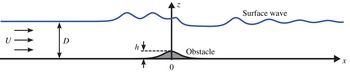
We consider a two-dimensional open channel flow over a hill-shaped obstacle (figure 1). The governing equations are the continuity equation for an incompressible fluid
 $$\begin{eqnarray}\unicode[STIX]{x1D735}\boldsymbol{\cdot }\boldsymbol{u}=0,\end{eqnarray}$$
and the Euler equations
 $$\begin{eqnarray}\frac{D\boldsymbol{u}}{Dt}=-\unicode[STIX]{x1D735}p-\frac{1}{Fr^{2}}\hat{\boldsymbol{z}},\end{eqnarray}$$
where
 $\boldsymbol{u}=(u,w)$
is the velocity with
 $u$
and
 $w$
being the horizontal and vertical component, respectively,
 $p$
is the pressure and
 $\hat{\boldsymbol{z}}$
is the unit vector in the vertical direction. We have used the channel depth
 $D$
as the length scale, the uniform upstream velocity
 $U$
as the velocity scale, and
 $\unicode[STIX]{x1D70C}U^{2}$
as the pressure scale. The Froude number
 $Fr$
is defined by (1.1).
Schematic figure of the problem.

The kinematic and the dynamic boundary conditions are imposed on the free surface. The kinematic condition is
 $$\begin{eqnarray}\frac{\unicode[STIX]{x2202}\unicode[STIX]{x1D702}}{\unicode[STIX]{x2202}t}+u\frac{\unicode[STIX]{x2202}\unicode[STIX]{x1D702}}{\unicode[STIX]{x2202}x}=w,\end{eqnarray}$$
where
 $\unicode[STIX]{x1D702}(x,t)$
is the vertical displacement of the free surface from its original height. The dynamic boundary condition which assures the stress balance is given by
 $$\begin{eqnarray}\displaystyle p=p_{0}+\frac{Bo}{Fr^{2}}\unicode[STIX]{x1D705}, & & \displaystyle\end{eqnarray}$$
where
 $p_{0}$
is the constant atmospheric pressure,
 $\unicode[STIX]{x1D705}$
is the local curvature of the free surface and the Bond number
 $Bo$
is defined by (1.1).
The shape of the obstacle on the bottom boundary is given by
 $z=h(x)$
, where
 $h(x)$
is given by
 $$\begin{eqnarray}h(x)=h_{0}\,\text{sech}^{2}(0.3x),\end{eqnarray}$$
with
 $h_{0}=0.02$
unless otherwise stated.
We solve the governing equations by the finite difference method, utilising the marker and cell (MAC) method (Harlow & Welch Reference Harlow and Welch1965) which has been used to solve the equations for an incompressible fluid. Since the top and bottom boundary are not straight in the present problem, we use the body-fitted curvilinear coordinates (Thompson, Thames & Mastin Reference Thompson, Thames and Mastin1974) so that the grid lines are always adjacent to the free surface and the bottom obstacle. The numerical method is essentially the same as in Hanazaki (Reference Hanazaki1992, Reference Hanazaki1993, Reference Hanazaki2003), except for the existence of the free surface which is the moving boundary.
In the spatial discretisation, the central difference of second-order accuracy is used except for the convection term, for which a third-order upwind scheme (Kawamura, Takami & Kuwahara Reference Kawamura, Takami and Kuwahara1986) is used to avoid the nonlinear computational instability which becomes significant in the flow with small viscosity.
For the time integration, second-order Adams–Bashforth method is used for the Euler equations, while the Crank–Nicolson method is used for the kinematic boundary condition (2.3) at the free surface. For the initial condition, impulsive start is used, i.e. the uniform velocity
 $(u,w)=(U,0)$
is given initially for the whole domain. We quit the computation well before the upstream waves reach the upstream boundary, so that any transparent boundary conditions do not become necessary. In all of the solutions of the Euler equations, the time increment is
 $\unicode[STIX]{x0394}t=2.0\times 10^{-4}$
, and the computation was continued until
 $t=400$
.
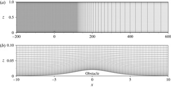
One of the two grids used for solving the Euler equations (
 $t=0$
). The total number of grid points of this grid is 19 000 (horizontal)
 $\times$
150 (vertical). (a) The perspective view of the grid (
 $-200\leqslant x\leqslant 600$
) where only every 100 grid points is depicted in the horizontal direction and every four grid points is depicted in the vertical direction. (b) The enlarged view of the grid near the obstacle (
 $-10\leqslant x\leqslant 10$
). Every 10 grid points is depicted in the horizontal direction.

The grid used for solving the Euler equations at low Bond numbers (
 $Bo<0.3$
) is shown in figure 2. In the upstream region and near the obstacle (
 $-200\leqslant x\leqslant 120$
), i.e. where short capillary waves appear, the minimum and constant grid size
 $(\unicode[STIX]{x0394}x)_{min}=0.02$
is used in the horizontal direction. Far downstream of the obstacle (
 $x\geqslant 120$
),
 $\unicode[STIX]{x0394}x$
is gradually increased. In the vertical direction the grid is concentrated near the free surface and the bottom boundary, giving the minimum grid size
 $(\unicode[STIX]{x0394}z)_{min}=0.005$
. At higher Bond numbers (
 $Bo\geqslant 0.3$
), another grid with lower resolution in the horizontal direction (
 $9500\times 150$
points) was used, since the wavelength of the short waves are longer.
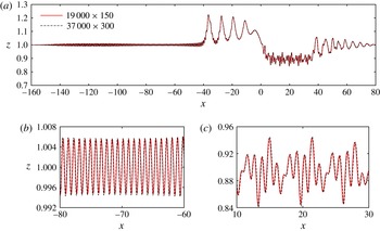
Since we solve the inviscid equations, it is important to check whether the effect of grid resolution on the numerical dissipation is negligible. The free-surface displacements obtained from the two computational grids at
 $Bo=0.15$
are presented in figure 3. The grid of
 $37\,000\times 300$
points has an approximately double resolution compared with the grid of
 $19\,000\times 150$
points (figure 2). The solutions obtained from the two grids have negligibly small difference in the overall wave patterns (figure 3
a), including the upstream long-wave solitary waves (
 $-40\lesssim x\lesssim 0$
) and the far downstream cnoidal waves (
 $x\gtrsim 40$
). The enlarged figures of the short waves confirm that both the upstream short waves (figure 3
b:
 $-80\lesssim x\lesssim -60$
) and the downstream short waves in the depression region (figure 3
c:
 $0\lesssim x\lesssim 40$
) show negligible difference. Therefore, we conclude that the
 $19\,000\times 150$
grid points is sufficient to resolve short waves observed at
 $Bo=0.15$
.
Since the wavelength of short waves is minimum at the lowest non-zero value of
 $Bo~(=0.15)$
investigated in this study, and it increases with
 $Bo$
, the accuracy at
 $Bo=0.15$
assures the accuracy at larger values of
 $Bo$
. Therefore, we have used the grid with
 $19\,000\times 150$
points (figure 2) for
 $0.15\leqslant Bo\leqslant 0.25$
. For higher Bond numbers (
 $Bo\geqslant 0.3$
) the grid with
 $9500\times 150$
points was used. It has a double horizontal grid size (
 $(\unicode[STIX]{x0394}x)_{min}=0.04$
), while the minimum vertical grid size is unchanged (
 $(\unicode[STIX]{x0394}z)_{min}=0.005$
), and the grid gave only negligible difference.
Most of the computations were performed using the NEC SX-ACE(256GFLOPS/node) in the Cybermedia Center, Osaka University.
Comparison of the surface wave patterns obtained by two grids with different resolutions (
 $Bo=0.15$
,
 $t=400$
). The solid line shows the result of the grid mainly used in this study (
 $19\,000\times 150$
points) and the dashed line shows the result of a grid which has approximately double resolution. The surface waves in the (a) wide region (
 $-160\leqslant x\leqslant 80$
), (b) upstream region (
 $-80\leqslant x\leqslant -60$
) and (c) downstream depression region (
 $10\leqslant x\leqslant 30$
).

2.2 Weakly nonlinear equations
The fKdV equation (e.g. Akylas Reference Akylas1984; Wu Reference Wu1987) for water waves without capillary effects has been derived to describe the nonlinear waves excited near resonant condition (
 $Fr\simeq 1$
), assuming that the horizontal coordinate
 $x$
, time
 $t$
, fluid surface displacement
 $\unicode[STIX]{x1D702}$
and the obstacle height
 $h$
are scaled as
 $$\begin{eqnarray}x=\unicode[STIX]{x1D700}^{-1/2}\unicode[STIX]{x1D709},\quad t=\unicode[STIX]{x1D700}^{-3/2}\unicode[STIX]{x1D70F},\quad \unicode[STIX]{x1D702}(x,t)=\unicode[STIX]{x1D700}A(\unicode[STIX]{x1D709},\unicode[STIX]{x1D70F})+O(\unicode[STIX]{x1D700}^{2}),\quad h(x)=\unicode[STIX]{x1D700}^{2}H(\unicode[STIX]{x1D709}),\end{eqnarray}$$
where
 $\unicode[STIX]{x1D700}$
is a small parameter. The fKdV equation under exact resonant condition (
 $Fr=1$
) then becomes
 $$\begin{eqnarray}-\frac{\unicode[STIX]{x2202}A}{\unicode[STIX]{x2202}\unicode[STIX]{x1D70F}}+\unicode[STIX]{x1D6FC}A\frac{\unicode[STIX]{x2202}A}{\unicode[STIX]{x2202}\unicode[STIX]{x1D709}}+\unicode[STIX]{x1D6FD}\frac{\unicode[STIX]{x2202}^{3}A}{\unicode[STIX]{x2202}\unicode[STIX]{x1D709}^{3}}+\frac{1}{2}\frac{\unicode[STIX]{x2202}H}{\unicode[STIX]{x2202}\unicode[STIX]{x1D709}}=0\left(\unicode[STIX]{x1D6FC}=\frac{3}{2},\unicode[STIX]{x1D6FD}=\frac{1-3Bo}{6}\right).\end{eqnarray}$$
We note that in the limit of
 $Bo\rightarrow 1/3$
, the dispersive term
 $\unicode[STIX]{x2202}_{x}^{3}\unicode[STIX]{x1D702}$
in the fKdV equation (2.7) vanishes, and the equation asymptotes to the inviscid Burgers equation (or the Hopf equation) which has a monotonic hydraulic-jump solution without a solitary wave (Grimshaw & Smyth Reference Grimshaw and Smyth1986). Therefore, in this parameter region (
 $Bo\simeq 1/3$
), a fifth-order fKdV equation with a fifth-order dispersive term (
 $\unicode[STIX]{x2202}_{x}^{5}\unicode[STIX]{x1D702}$
) has been proposed (Milewski & Vanden-Broeck Reference Milewski and Vanden-Broeck1999). It can be derived using different scalings, i.e.
 $$\begin{eqnarray}x=\unicode[STIX]{x1D700}^{-1/4}\unicode[STIX]{x1D709},\quad \hspace{-1.0pt}t=\unicode[STIX]{x1D700}^{-5/4}\unicode[STIX]{x1D70F},\quad \hspace{-1.0pt}\unicode[STIX]{x1D702}(x,t)=\unicode[STIX]{x1D700}A(\unicode[STIX]{x1D709},\unicode[STIX]{x1D70F})+O(\unicode[STIX]{x1D700}^{2}),\quad \hspace{-1.0pt}h(x)=\unicode[STIX]{x1D700}^{2}H(\unicode[STIX]{x1D709}),\quad \unicode[STIX]{x1D6FD}=-{\textstyle \frac{1}{2}}\unicode[STIX]{x1D700}^{1/2}\unicode[STIX]{x0394}_{Bo}.\end{eqnarray}$$
Here, the new scaling for the horizontal length (
 $x\sim \unicode[STIX]{x1D700}^{-1/4}$
) suggests shorter wavelength than the fKdV equation which assumed
 $x\sim \unicode[STIX]{x1D700}^{-1/2}$
. We also note that
 $\unicode[STIX]{x1D6FD}$
is scaled by
 $\unicode[STIX]{x1D700}^{1/2}$
and not by
 $\unicode[STIX]{x1D700}$
or
 $\unicode[STIX]{x1D700}^{2}$
, meaning that the applicable range of
 $|\unicode[STIX]{x1D6FD}|$
and
 $Bo$
might not be necessarily very small. For example, if we assume
 $\unicode[STIX]{x1D700}=0.1$
and
 $|\unicode[STIX]{x0394}_{Bo}|=1$
,
 $|\unicode[STIX]{x1D6FD}|$
becomes 0.16, giving a wide range of
 $Bo$
, i.e.
 $0.013\leqslant Bo\leqslant 0.65$
.
Under the exact resonant condition (
 $Fr=1$
), the equation becomes
 $$\begin{eqnarray}-\frac{\unicode[STIX]{x2202}A}{\unicode[STIX]{x2202}\unicode[STIX]{x1D70F}}+\unicode[STIX]{x1D6FC}A\frac{\unicode[STIX]{x2202}A}{\unicode[STIX]{x2202}\unicode[STIX]{x1D709}}-\frac{1}{2}\unicode[STIX]{x0394}_{Bo}\frac{\unicode[STIX]{x2202}^{3}A}{\unicode[STIX]{x2202}\unicode[STIX]{x1D709}^{3}}+\unicode[STIX]{x1D6FE}\frac{\unicode[STIX]{x2202}^{5}A}{\unicode[STIX]{x2202}\unicode[STIX]{x1D709}^{5}}+\frac{1}{2}\frac{\unicode[STIX]{x2202}H}{\unicode[STIX]{x2202}\unicode[STIX]{x1D709}}=0\left(\unicode[STIX]{x1D6FE}=\frac{1}{90}\right).\end{eqnarray}$$
In this study, in solving the fKdV and the fifth-order KdV equations, the scaled variables
 $\unicode[STIX]{x1D709},\unicode[STIX]{x1D70F},A$
and
 $H$
are turned back to the original variables
 $x,t,\unicode[STIX]{x1D702}$
and
 $h$
so that the comparison with the Euler equations becomes easier.
Namely, we have solved
 $$\begin{eqnarray}-\frac{\unicode[STIX]{x2202}\unicode[STIX]{x1D702}}{\unicode[STIX]{x2202}t}+\unicode[STIX]{x1D6FC}\unicode[STIX]{x1D702}\frac{\unicode[STIX]{x2202}\unicode[STIX]{x1D702}}{\unicode[STIX]{x2202}x}+\unicode[STIX]{x1D6FD}\frac{\unicode[STIX]{x2202}^{3}\unicode[STIX]{x1D702}}{\unicode[STIX]{x2202}x^{3}}+\frac{1}{2}\frac{\unicode[STIX]{x2202}h}{\unicode[STIX]{x2202}x}=0,\end{eqnarray}$$
and
 $$\begin{eqnarray}-\frac{\unicode[STIX]{x2202}\unicode[STIX]{x1D702}}{\unicode[STIX]{x2202}t}+\unicode[STIX]{x1D6FC}\unicode[STIX]{x1D702}\frac{\unicode[STIX]{x2202}\unicode[STIX]{x1D702}}{\unicode[STIX]{x2202}x}+\unicode[STIX]{x1D6FD}\frac{\unicode[STIX]{x2202}^{3}\unicode[STIX]{x1D702}}{\unicode[STIX]{x2202}x^{3}}+\unicode[STIX]{x1D6FE}\frac{\unicode[STIX]{x2202}^{5}\unicode[STIX]{x1D702}}{\unicode[STIX]{x2202}x^{5}}+\frac{1}{2}\frac{\unicode[STIX]{x2202}h}{\unicode[STIX]{x2202}x}=0,\end{eqnarray}$$
as the fKdV equation and the fifth-order KdV equation, respectively.
We have applied the horizontally periodic boundary condition, and the Fourier-spectral method is used for the spatial discretisation. The fourth-order Runge–Kutta method is used for the time development. We note that there is no
 $\unicode[STIX]{x1D700}$
in equations (2.10) and (2.11), and the solutions do not depend on
 $\unicode[STIX]{x1D700}$
, although the accuracy of approximation is higher for smaller
 $\unicode[STIX]{x1D700}$
.
3 Results
3.1 Capillary effects
We first show the behaviour of the gravity wave without capillary effects (
 $Bo=0$
). Time development of the free-surface displacement
 $\unicode[STIX]{x1D702}(x,t)$
obtained from the Euler equations (figure 4
a) shows that the waves resonantly excited by an obstacle grow up into a train of solitary waves which propagates upstream of the obstacle (
 $x<0$
), while the modulated cnoidal waves appear downstream of the obstacle (
 $x>0$
). At the same time, a flat depression appears between the obstacle and the cnoidal waves. It elongates with time, compensating for the upstream surface elevation by the solitary waves and assuring the mass conservation of the fluid. These processes can be described well by the fKdV equation (e.g. Grimshaw & Smyth Reference Grimshaw and Smyth1986), not only qualitatively but also quantitatively (figure 4
b), as long as the assumption of long wave and small amplitude, i.e. small
 $\unicode[STIX]{x1D716}(\ll 1)$
, is satisfied.


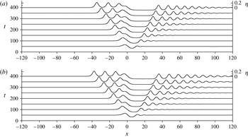
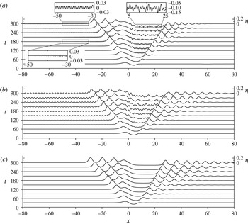
We next show the surface waves with capillary effects. Figure 5(a) shows the wave development obtained by the Euler equations at the smallest non-zero Bond number (
 $Bo=0.15$
). An important effect of the capillary force is the generation of short waves whose wavelengths are comparable with the fluid depth. They appear upstream of the foremost solitary wave and downstream of the depression region. The upstream short waves have constant wavelengths and amplitudes, and they advance at a constant speed without changing their form, while the downstream short waves look highly irregular. The short waves appear also on long waves, overlapping the upstream solitary waves and the downstream cnoidal waves.


Figure 5(b,c) shows the free-surface development (
 $Bo=0.15$
) obtained from the fifth-order fKdV equation and the fKdV equation. While the fKdV equation (figure 5
c) predicts only the long solitary waves and the cnoidal waves, the fifth-order fKdV equation (figure 5
b) generates also the short waves. Similar wave patterns to figure 5(b) have been obtained by Milewski & Vanden-Broeck (Reference Milewski and Vanden-Broeck1999), solving the fifth-order fKdV equation with a modified dispersion term which does not change the accuracy of the original equation. They named the modified equation as forced BBM5, since the relation between the fifth-order fKdV equation and their modified equation is similar to the relation between the KdV equation and the Benjamin–Bona–Mahoney equation. We note, however, that the BBM5 cannot be used in the exactly resonant case (
 $Fr=1$
), since the modified dispersion terms diverge.
Time development of the free-surface displacement
 $\unicode[STIX]{x1D702}(x,t)$
at
 $Bo=0.15$
: (a) Euler equations; (b) fifth-order fKdV equation.

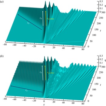
To investigate the generation process of the upstream short waves, bird’s-eye views of figure 5(a,b) are presented in figure 6. The wave crests of the upstream short waves are straight and parallel to the crests of the solitary waves, showing that the short waves have a constant phase speed
 $c_{p}$
equal to that of the solitary waves (
 $=c_{p\;soliton}$
). This shows that the upstream solitary waves emit short waves whose phase speed is equal to the solitary wave, as is typical to the ‘resonant radiation’ observed when a fifth-order dispersive term is added to the KdV equation (e.g., Karpman Reference Karpman1998).
We observe that the upstream short waves appear initially on the upstream slope of the foremost solitary wave and their existing region spreads upstream ahead of the solitary wave. This would occur when the group speed of the short waves (
 $=c_{g}$
) is faster than their phase speed. Actually, in the fifth-order fKdV equation, the group of short waves moves upstream much faster than the Euler equations. The relation between the group velocity and the phase velocity and the significant difference in the group velocity between the Euler equations and the fifth-order fKdV equation, are explained by the dispersion relations which will be shown in figure 7.
The fifth-order fKdV equation gives solutions qualitatively similar to the Euler equations in that its phase velocity
 $c_{p}$
is equal to that of the solitons (
 $=c_{p\;soliton}$
), there are noticeable quantitative differences between them (cf. figures 5
a,b and 6). First, the fifth-order fKdV equation overestimates the wavelength and amplitude of the short waves. Second, it overestimates the group speed
 $c_{g}$
significantly. These differences would be attributable to the long-wave approximation used in the fifth-order fKdV equation, which makes large difference in the dispersion relation. The linear dispersion relation for the Euler equation can be obtained by substituting
 $\text{e}^{\text{i}(kx-\unicode[STIX]{x1D714}t)}$
into the linearised Euler equation, and the frequency of the component which propagates upstream in quiescent fluid is given by
 $$\begin{eqnarray}\displaystyle \unicode[STIX]{x1D714}(k)=k-\sqrt{(k+Bok^{3})\tanh k} & & \displaystyle\end{eqnarray}$$
in the reference frame of the stationary obstacle. Here,
 $\unicode[STIX]{x1D714}$
is the frequency and
 $k$
is the horizontal wavenumber. On the other hand, the dispersion relation for the linearised fifth-order fKdV equation is
 $$\begin{eqnarray}\displaystyle \unicode[STIX]{x1D714}(k)=\unicode[STIX]{x1D6FD}k^{3}-\unicode[STIX]{x1D6FE}k^{5}. & & \displaystyle\end{eqnarray}$$
The dispersion relation (3.2) can be deduced alternatively from the Taylor expansion of (3.1) assuming small
 $k$
 $({\sim}\unicode[STIX]{x1D700}^{1/4})$
and
 $|Bo-1/3|$
 $({\sim}\unicode[STIX]{x1D700}^{1/2})$
as in the derivation of the fifth-order fKdV equation (cf. (2.8)), and truncating the expansion at the order of
 $\unicode[STIX]{x1D700}^{5/4}$
.
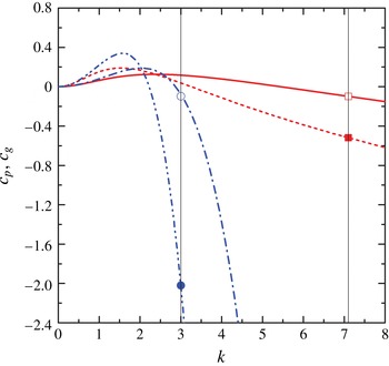
The phase velocity
 $c_{p}(k)$
and the group velocity
 $c_{g}(k)$
relative to the obstacle obtained from the linear dispersion relations for the Euler equation (3.1) (
 $c_{p}$
: ——,
 $c_{g}$
: - - - - -) and the fifth-order fKdV equation (3.2) (
 $c_{p}$
: — - — -,
 $c_{g}$
: — - - — - -) at
 $Bo=0.15$
(
 $Fr=1$
). In the long-wave limit,
 $c_{p}(0)=c_{g}(0)=0$
is satisfied since
 $Fr=1$
. The two open symbols show the wavenumber and the phase velocity of the upstream short waves actually observed in the solutions of the Euler equations (▫) and the fifth-order fKdV equation (○). The closed symbols (▪, ●) show the observed group velocities of the same waves.

In figure 7, we plot the phase speed
 $c_{p}(k)$
and the group speed
 $c_{g}(k)$
calculated by (3.1) and (3.2). The curves for the Euler equations and the fifth-order fKdV equation agree at low wavenumbers (
 $k\ll 1$
), but they differ significantly at larger
 $k$
. The upstream short waves observed in the Euler and the fifth-order fKdV equations, denoted by open symbols, have almost the same phase speed. This suggests that both short waves are generated by the resonant radiation, and have the phase velocity equal to the upstream-advancing speeds of the solitary wave, which are almost equal in the Euler equations and the fifth-order fKdV equation (cf. figure 6). The open symbols are almost on each theoretical
 $c_{p}(k)$
curve, showing that the small-amplitude short waves satisfy the linear dispersion relation. However, the two curves for
 $c_{p}(k)$
are widely separated at high wavenumbers (
 $k\gtrsim 2.5$
), and the wavenumber observed in the Euler equations is much larger than that observed in the fifth-order fKdV equation as already noted in figures 5 and 6.
The closed symbols which represent the measured wavenumber and group velocity are also on the theoretical curves of
 $c_{g}(k)$
, confirming that the short waves are the linear waves. However, the large difference in the wavenumber and
 $c_{g}(k)$
curve results in the much faster upstream-propagating group velocity in the fifth-order fKdV equation, as we have observed in figures 5 and 6.
3.2 Bond-number dependence
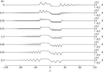
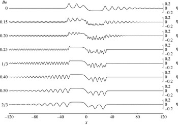
To observe the Bond number dependence of the wave patterns, free-surface displacements
 $\unicode[STIX]{x1D702}(x,t)$
obtained from the Euler equations are presented in figure 8. It shows that short waves of small amplitude appear upstream of the solitary waves when
 $Bo$
is a small non-zero value (e.g.
 $Bo=0.15$
, cf. figures 5
a, 6
a), and both the wavelength and the amplitude asymptote to zero in the limit of
 $Bo\rightarrow 0$
. The solutions for very low Bond numbers (
 $0<Bo<0.15$
) are not pursued in this paper, since the extremely short waves certainly inhibit the accurate numerical solution.
Free-surface displacements
 $\unicode[STIX]{x1D702}(t,x)$
at
 $t=300$
obtained by the Euler equations.

Free-surface displacements
 $\unicode[STIX]{x1D702}(t,x)$
at
 $t=300$
obtained by the fKdV equation (
 $Bo=0$
) and the fifth-order fKdV equation (
 $Bo>0$
).

With the increasing Bond number, the downstream depression region changes into depression solitary waves which propagate downstream. At the same time, the wavelength and the amplitude of the upstream short waves increase, and they finally change into cnoidal waves. We note that the wave pattern at
 $Bo=2/3$
almost agrees with that at
 $Bo=0$
by a
 $180^{\circ }$
rotation around the origin
 $(x,\unicode[STIX]{x1D702})=(0,0)$
. This point symmetry holds exactly in the fKdV equation, since the equation (2.10) is invariant against the transform of variables given by
 $\unicode[STIX]{x1D702}\rightarrow -\unicode[STIX]{x1D702}$
,
 $x\rightarrow -x$
and
 $Bo\rightarrow 2/3-Bo$
(i.e.
 $\unicode[STIX]{x1D6FD}\rightarrow -\unicode[STIX]{x1D6FD}$
). The fifth-order fKdV equation (2.11) does not have this symmetry due to the fifth-order derivative term
 $\unicode[STIX]{x1D6FE}\unicode[STIX]{x2202}^{5}\unicode[STIX]{x1D702}$
. However, the short waves do not appear at the large Bond number of
 $Bo=2/3$
, and the point symmetry is retained.
At small Bond numbers (
 $0<Bo\lesssim 0.25$
), short waves appear also in the downstream depression region, but they look irregular in space and time, as observed in figure 5(a). They have larger wavelength and amplitude at larger Bond numbers, and finally at
 $Bo=2/3$
change into the reversed solitary waves which have been observed as positive solitary waves in the upstream region at
 $Bo=0$
.
Figure 9 shows the corresponding free-surface displacements obtained from the fifth-order fKdV equation. In the case of
 $Bo=0$
, however, solution of the fKdV equation is presented instead of the fifth-order fKdV equation. The latter equation produces unrealistic short waves, although the long-wave aspects of the flow, such as the upstream solitary wave train and the downstream depression, agree with the fKdV equation, and the maximum amplitude of the short waves is very small (
 ${\sim}2.5\times 10^{-4}$
). Comparison with figure 8 shows that the long waves are described well by the fifth-order fKdV equation (
 $0.15\leqslant Bo\leqslant 2/3$
) or by the fKdV equation (
 $Bo=0$
). At the lowest and the highest Bond numbers for which short waves do not appear in the Euler equations (
 $Bo=0$
and
 $Bo=2/3$
), quantitative comparison is very good. The appearance of upstream short waves at small non-zero Bond numbers (
 $0<Bo\lesssim 1/3$
) are also predicted by the fifth-order fKdV equation. However, their wavelengths and the corresponding upstream-advancing speeds (i.e. group velocities) are generally overestimated as discussed in figure 7.
3.3 Short waves in the downstream depression region
We next examine the short waves which appear in the downstream depression region, i.e. between the obstacle (
 $x\approx 0$
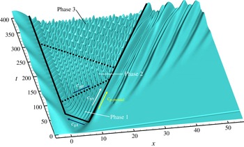
) and the downstream cnoidal waves. A bird’s-eye view of the time development of free-surface displacement
 $\unicode[STIX]{x1D702}(x,t)$
in the depression region is shown in figure 10 (
 $Bo=0.15$
), which gives an enlarged view of figures 5(a) and 6(a). The short waves initially appear at
 $t\sim 30$
on the upstream slope (
 $x\sim 5$
) of the cnoidal wave. Their wave crests are parallel to those of cnoidal waves, showing that their phase velocity
 $c_{pA}$
is equal to the phase velocity of the cnoidal wave (
 $=c_{p\;cnoidal}$
). Their existing region spreads upstream at its group velocity
 $c_{gA}$
until
 $t\sim 110$
. In this initial stage (phase 1), the short waves have straight wave crests, suggesting that only one wavenumber component which propagates at a constant speed is generated.
Time development of the free-surface displacement
 $\unicode[STIX]{x1D702}(x,t)$
in the downstream depression region (Euler equations,
 $Bo=0.15$
).

After
 $t\sim 110$
(phase 2), the waves begin to take a mesh pattern, and the new pattern spreads downstream at a constant group velocity (
 $=c_{gB}$
) along the lower dashed line in figure 10. This suggests that the new short waves, generated by the interaction between the original short wave and the long wave just over the obstacle, are released downstream. Then, the waves in the depression region become the superposition of two waves whose group velocities are in the opposite direction. This explains why these waves looked irregular at large times in figure 5(a).
Finally after
 $t\sim 220$
(phase 3), the wave pattern becomes more complicated, suggesting that the third wave component is produced by the downstream cnoidal waves. The third component propagates upstream and a new wave pattern spreads upstream until it approaches the obstacle at
 $t\sim 320$
.
The results suggest that the wave pattern will become further complicated as the new components are successively generated by the interaction between the short waves and the long waves. In this study, however, the computation is ceased at
 $t=400$
since a longer time integration requires a high grid resolution further upstream of the obstacle.
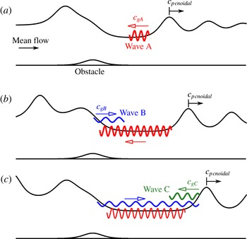
A presumable time sequence of the short-wave generation is illustrated in figure 11. In phase 1, wave A is radiated from the downstream cnoidal wave (figure 11 a). Its existing region spreads upstream and approaches the obstacle. In phase 2, wave B is generated by the interaction between wave A and the long wave above the obstacle (figure 11 b), and wave B advances downstream until it meets the cnoidal wave. In phase 3, wave C is generated by the interaction between wave B and the cnoidal wave and it propagates upstream (figure 11 c). These processes will continue, and the number of wave components will increase in a long time evolution.
Schematic of the generation process of downstream short waves. (a) Phase 1: wave A is radiated from the cnoidal wave and propagates upstream at its group velocity
 $c_{gA}$
. (b) Phase 2: wave B is generated by the interaction between wave A and the long wave above the obstacle, and it propagates downstream at the group velocity
 $c_{gB}$
. (c) Phase 3: wave C is generated by the interaction between wave B and the cnoidal wave, and it propagates upstream at the group velocity
 $c_{gC}$
.

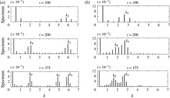
Wavenumber spectra in the depression region at
 $t=100$
, 200 and 375. A space discrete Fourier transform (space-DFT) is applied to the depression region, using a hamming window function: (a)
 $Bo=0.15$
; (b)
 $Bo=0.25$
.

Peak wavenumbers
 $k_{A}$
,
 $k_{B}$
and
 $k_{C}$
obtained by space-DFT in the depression region for various Bond numbers (
 $t=375$
).


To investigate the short waves in the depression region in more detail, we examine the wave spectra in figure 12. At
 $Bo=0.15$
(figure 12
a), the first peak at
 $k_{A}=5.9$
(wave A) appears by
 $t=100$
, the second peak at
 $k_{B}=2.0$
(wave B) appears by
 $t=200$
and the third peak at
 $k_{C}=4.8$
(wave C) appears by
 $t=375$
. At
 $Bo=0.25$
(figure 12
b), only two peaks
 $k_{A}$
and
 $k_{B}$
appear by
 $t=375$
since the wavenumbers (
 $k_{A}$
and
 $k_{B}$
) are smaller and the absolute values of the corresponding group velocities (
 $|c_{gA}|$
and
 $|c_{gB}|$
) are slower at higher Bond numbers (cf. figures 13 and 14). Although the spectral peaks are not sharp, these results support the conjecture in figure 10 that the short waves in the depression region are the superposition of the components generated successively at the upstream and downstream ends of the depression region.
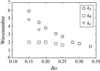
The peak wavenumbers
 $k_{A}$
,
 $k_{B}$
and
 $k_{C}$
observed at
 $t=375$
for all of the Bond numbers investigated in this study are plotted in figure 13. As
 $Bo$
increases,
 $k_{A}$
and
 $k_{C}$
become smaller, while
 $k_{B}$
changes slightly. For large
 $Bo$
, the number of spectrum peak observed at
 $t=375$
decreases.
To examine the behaviour of short waves, we need to reconsider the linear dispersion relation. In the depression region, the fluid is shallower than the upstream region and the mean flow speed is larger than unity. Then, we use a dispersion relation with a modified water depth
 $D_{d}~({<}1)$
and a modified mean flow speed
 $U_{d}~({>}1)$
, i.e.
 $$\begin{eqnarray}\displaystyle \unicode[STIX]{x1D714}=U_{d}k-\sqrt{(k+Bok^{3})\tanh (kD_{d})}. & & \displaystyle\end{eqnarray}$$
When we use (3.3) in the following analysis,
 $D_{d}$
is obtained by averaging the fluid depth over
 $5<x<25$
at
 $t=375$
, while
 $U_{d}$
is obtained by averaging the horizontal velocity over
 $x$
and
 $z$
at
 $t=375$
, or simply from
 $U_{d}D_{d}=1$
. Since the fluctuation of fluid depth and the horizontal velocity in the depression region is small compared with the total depth and velocity,
 $D_{d}$
and
 $U_{d}$
so obtained would assure trustful usage of the dispersion relation.
In the case of
 $Bo=0.15$
, for example, the mean values of
 $D_{d}$
and
 $U_{d}$
in the depression region at
 $t=375$
are
 $D_{d}=0.90$
and
 $U_{d}=1/D_{d}=1.1$
. The wavenumber
 $k_{A}(=5.9)$
or the wavelength
 $\unicode[STIX]{x1D706}_{A}=2\unicode[STIX]{x03C0}/k_{A}=1.06$
obtained from the wave pattern in figure 10 and from the Fourier transform given in figure 12 agrees. Substitution of this wavenumber into the dispersion relation (3.3) gives the phase velocity
 $c_{pA}=\unicode[STIX]{x1D714}/k_{A}=0.083$
. This agrees with the phase velocity obtained directly from figure 10, which is also equal to the moving speed of the cnoidal wave (
 $c_{pA}=c_{p\;cnoidal}$
). This shows that wave A obeys the linear dispersion relation and it is a linear wave.
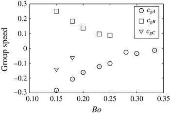
Figure 14 shows the group velocity obtained from the differential of the modified dispersion relation (3.3), using the wavenumber given in figure 13. In the case of
 $Bo=0.15$
,
 $c_{gA}=-0.27({<}0)$
, meaning that the energy of wave A propagates upstream. This is consistent with
 $c_{gA}$
in phase 1 of figures 10 and 11(a).
Frequency spectra of the surface displacement
 $\unicode[STIX]{x1D702}$
in the depression region (at
 $x=20$
) obtained by time-DFT in the period of
 $250\leqslant t\leqslant 400$
: (a)
 $Bo=0.15$
; (b)
 $Bo=0.25$
.

Peak frequencies (
 $\unicode[STIX]{x1D714}_{1}$
and
 $\unicode[STIX]{x1D714}_{2}$
) of the surface displacement
 $\unicode[STIX]{x1D702}$
in the depression region (at
 $x=20$
) obtained by time-DFT for various Bond numbers (
 $0.15\leqslant Bo\leqslant 1/3$
) in the period of
 $250\leqslant t\leqslant 400$
.

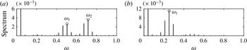
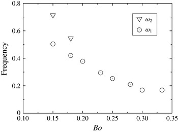
Figure 15 shows the frequency spectrum in the depression region obtained by time discrete Fourier transform (time-DFT), and figure 16 shows the peak frequencies observed at various Bond numbers (
 $0.15\leqslant Bo\leqslant 1/3$
). One of the two values of
 $\unicode[STIX]{x1D714}$
(
 $\unicode[STIX]{x1D714}_{1}\simeq 0.5$
) observed at
 $Bo=0.15$
(figures 15
a and 16) agrees with the value obtained by substituting
 $k_{A}=5.9$
into the linear dispersion relation (3.6), i.e.
 $\unicode[STIX]{x1D714}_{A}=c_{pA}k_{A}=0.083\times 5.9=0.49$
, confirming that wave A is a linear wave.
In phase 2, another wavenumber
 $k_{B}=2.0$
appears in the spectrum (figure 12(a),
 $t=200$
). Substituting this value into the linear dispersion relation (3.3) gives
 $\unicode[STIX]{x1D714}_{B}=0.48$
, which agrees with the direct observation of frequency (
 $\unicode[STIX]{x1D714}_{1}\simeq 0.5$
) in figure 15(a). Applicability of the linear dispersion relation shows that wave B is also a linear wave.
We also note that this frequency is equal to the frequency of wave A. Other than
 $\unicode[STIX]{x1D714}_{2}$
which would be the frequency of wave C, we observe only
 $\unicode[STIX]{x1D714}_{1}=0.5$
in figures 15(a) and 16. As described above, both the linear dispersion relation and the direct observation give the frequency of wave A as
 $\unicode[STIX]{x1D714}_{A}\simeq \unicode[STIX]{x1D714}_{1}=0.5$
which is nearly equal to
 $\unicode[STIX]{x1D714}_{B}$
. This suggests that wave B is generated by the interaction between wave A and another wave with a very small frequency
 $\unicode[STIX]{x1D714}_{0}~(\ll \unicode[STIX]{x1D714}_{A})$
, since the frequencies would satisfy the relation
 $\unicode[STIX]{x1D714}_{B}=\unicode[STIX]{x1D714}_{A}+\unicode[STIX]{x1D714}_{0}$
. Considering that wave A propagates upstream and reaches the obstacle at
 $x=0$
, it is natural to infer that wave A interacts with the nearly steady wave just above the obstacle whose frequency is
 $\unicode[STIX]{x1D714}_{0}~(\ll \unicode[STIX]{x1D714}_{A})$
and generate wave B. Since the group velocity of wave B (
 $k_{B}=2.0$
) estimated by (3.3) is
 $c_{gB}=0.27({>}0)$
(figure 14), its energy propagates downstream. This is consistent with phase 2 of figure 10, which shows that the mesh pattern extends downstream.
In phase 3, wave C (
 $k_{C}=4.8$
) appears in figure 12(a) (
 $t=375$
), and three wave components coexist. If the interaction of wave B with the cnoidal wave generates wave C, while the cnoidal wave moves downstream at the speed of
 $c_{cnoidal}$
, the frequency and the wavenumber would satisfy the relation
 $$\begin{eqnarray}\unicode[STIX]{x1D714}_{C}=\unicode[STIX]{x1D714}_{B}+\unicode[STIX]{x1D714}_{cnoidal},\quad k_{C}=k_{B}+k_{cnoidal}.\end{eqnarray}$$
If the phase velocity of the cnoidal wave (
 $=c_{p\;cnoidal}$
) satisfies
 $$\begin{eqnarray}\unicode[STIX]{x1D714}_{cnoidal}=c_{p\;cnoidal}\times k_{cnoidal},\end{eqnarray}$$
equations (3.4) and (3.5) lead to
 $$\begin{eqnarray}\unicode[STIX]{x1D714}_{C}=\unicode[STIX]{x1D714}_{B}+c_{p\;cnoidal}(k_{C}-k_{B}),\end{eqnarray}$$
or
 $$\begin{eqnarray}\unicode[STIX]{x1D714}_{C}^{d}=\unicode[STIX]{x1D714}_{B}^{d},\end{eqnarray}$$
with the definition of
 $\unicode[STIX]{x1D714}_{B}^{d}\equiv \unicode[STIX]{x1D714}_{B}-c_{p\;cnoidal}\times k_{B}$
and
 $\unicode[STIX]{x1D714}_{C}^{d}\equiv \unicode[STIX]{x1D714}_{C}-c_{p\;cnoidal}\times k_{C}$
.
Substitution of
 $c_{p\;cnoidal}=c_{pA}=0.083$
,
 $k_{B}=2.0$
and
 $k_{C}=4.8$
into (3.6) gives
 $\unicode[STIX]{x1D714}_{C}=0.48+0.083\times (4.8{-}2.0)=0.71$
, while the direct observation gives
 $\unicode[STIX]{x1D714}_{2}=0.71~(\simeq \unicode[STIX]{x1D714}_{C})$
. This agreement shows that wave C is generated by the interaction between wave B and the cnoidal wave.
Similar generation of waves by the interaction between nonlinear waves and dispersive waves has been known in optics. For example, Skryabin & Yulin (Reference Skryabin and Yulin2005) investigated the generation of waves by the mixing of solitons and dispersive waves in a optical fiber. They considered the generalised nonlinear Schrödinger (NLS) equation with higher-order dispersive terms, and confirmed the interaction of waves in experiments (Efimov et al. Reference Efimov, Yulin, Skryabin, Knight, Joly, Omenetto, Taylor and Russell2005).
4 Conclusions
We have investigated capillary–gravity waves resonantly excited by an obstacle (
 $Fr=1$
), and observed the radiation of short waves from the long waves when the Bond number is small
 $(0.15\leqslant Bo<1/3)$
. The upstream-advancing solitary waves radiate short waves whose phase velocity is equal to the solitary waves but group velocity is faster than the solitary waves. Then, the short waves are observed upstream of the foremost solitary wave. The short waves generally have much smaller amplitude than the solitary waves and they are essentially the linear waves.
Downstream of the obstacle, the cnoidal wave also radiates a short wave whose phase velocity is equal to the cnoidal wave and group velocity is negative, i.e. in the upstream direction. Then, the generated short wave is observed in the depression region between the obstacle and the cnoidal wave. The generation mechanism of the downstream short wave is essentially the same as the upstream short wave.
When the short wave radiated by the cnoidal wave arrives at the obstacle, it interacts with the nearly steady long wave over the obstacle and generates a second short wave which propagates downstream at its positive group velocity. This second short wave propagates until it reaches the downstream cnoidal wave with which it interacts to generate a third short wave. The third short wave, if it exists, has a negative group velocity and propagates upstream. These processes will continue, and the number of wavenumber components will increase in the depression region to generate an increasingly complicated wave pattern.
The same phenomenon might be observed at lower Bond numbers (
 $0<Bo<0.15$
), but the wavelength of the upstream short waves becomes extremely short and the group velocity becomes very fast. Then, a very fine numerical grid in a very wide region becomes necessary, so that the accurate numerical solution becomes almost impossible. In experiments, effects of viscosity should become significant for short waves and those waves may decay in a very short time. In spite of these difficulties, it is an interesting future problem to know at which Bond number the short waves cease to be observed, as the decreasing Bond number reduces the amplitude of the short waves.
For larger Bond numbers (
 $1/3\leqslant Bo\leqslant 2/3$
), the upstream solitons change into monotonic bores and when the wave pattern has almost a point symmetry against the origin (
 $(x,\unicode[STIX]{x1D702})=(0,0)$
) at
 $Bo=2/3$
, the monotonic bore is the counterpart of the downstream depression observed at low Bond numbers. Upstream short waves have longer wavelength and larger amplitude for larger
 $Bo$
, and they deform into cnoidal waves of opposite sign. The waves in the depression region also become longer for larger
 $Bo$
, and they finally become negative solitary waves, which are the counterpart of the upstream positive solitary waves observed at low Bond numbers.
The soliton radiation upstream of the solitary waves can be qualitatively described by the fifth-order fKdV equation, but the equation significantly overestimates the wavelength and the upstream-advancing group velocity since it is based on a long-wave approximation. The equation and the fKdV equation give quantitatively good approximations at
 $Bo=0$
and
 $2/3$
, for which the effect of the fifth-order derivative term is not significant.
In this study, the obstacle height (
 $h_{0}=0.02$
) and the Froude number (
 $Fr=1$
) are fixed. The effect of these parameters should be investigated in the subsequent study, but we can discuss the plausible effects. If the obstacle height
 $h_{0}$
is higher (
 $h_{0}>0.02$
), the amplitude of the solitary wave would become larger. Then, the short waves of higher amplitude might be generated, as predicted by Karpman (Reference Karpman1998). For a negative height (
 $h_{0}<0$
), complicated behaviour of solitary waves near the origin (
 $x=0$
) have been predicted by the solution of the fKdV equation (Grimshaw & Smyth Reference Grimshaw and Smyth1986). In that case also, short waves might be generated, and their amplitude might be large if the amplitude of the solitary wave is large.
If the Froude number decreases from unity (
 $Fr<1$
), the amplitude of the solitary waves becomes smaller, while the upstream-advancing speed becomes faster due to the linear effects. We can expect that the amplitude of the short waves would become smaller due to the smaller solitary waves. On the other hand, if the Froude number increases slightly (
 $Fr>1$
) but the flow is still resonant, the amplitude of the solitary waves becomes even larger than the case of
 $Fr=1$
(Grimshaw & Smyth Reference Grimshaw and Smyth1986). In that case, the amplitude of the short waves might become larger. If the Froude number further increases and the flow becomes non-resonant, the amplitude of the solitary wave would become much smaller, and the short waves would not be generated.
We should comment on the relation between the parameters used in this study and the real fluid. If we consider water at
 $20\,^{\circ }\text{C}$
and assume
 $Bo=0.15$
, the definition of the Bond number in (1.1), i.e.
 $Bo=T/\unicode[STIX]{x1D70C}gD^{2}$
, gives the fluid depth as
 $D=0.7~\text{cm}$
, since the surface tension
 $T$
of water at
 $20^{\circ }C$
is
 $0.073~\text{N}~\text{m}^{-1}$
, density
 $\unicode[STIX]{x1D70C}$
is
 $1.0\times 10^{3}~\text{kg}~\text{m}^{-3}$
, and the acceleration due to gravity is
 $g=9.8~\text{m}~\text{s}^{-2}$
. Then, if we fix the Froude number at
 $Fr=1$
, the definition of the Froude number in (1.1), i.e.
 $Fr=U/\sqrt{gD}$
, gives the uniform mean flow velocity as
 $U=26~\text{cm}~\text{s}^{-1}$
. These values of
 $D$
and
 $U$
and the dynamic viscosity coefficient
 $\unicode[STIX]{x1D708}=0.01~\text{cm}^{2}~\text{s}^{-1}$
give the Reynolds number
 $Re_{D}=UD/\unicode[STIX]{x1D708}$
as 1800. For a larger Bond number,
 $D$
and
 $U$
decrease and
 $Re_{D}$
decreases. For the largest Bond number
 $(=2/3)$
investigated in this study, the Reynolds number takes a lower value of
 $Re_{D}=600$
.
We finally note that the time scale for the viscous damping of the wave is estimated by
 $t\sim 1/\unicode[STIX]{x1D708}k^{2}$
in dimensional form. The shortest wave in this study is observed at
 $Bo=0.15$
, for which the dimensional wavenumber becomes
 $k\sim 7/D=10~\text{cm}^{-1}$
, using the non-dimensional wavenumber
 $k\sim 7$
in figure 7 and
 $D=0.7~\text{cm}$
as described above. Then, using the dynamic viscosity coefficient
 $\unicode[STIX]{x1D708}=0.01~\text{cm}^{2}~\text{s}^{-1}$
, the dissipation time scale becomes
 $t\sim 1~\text{s}$
, or
 $Ut/D=26~\text{cm}~\text{s}^{-1}\times 1~\text{s}/0.7~\text{cm}=3.7$
in its non-dimensional form. This is significantly small compared with the time scale for which the upstream solitary waves can develop (
 $Ut/D\sim 100$
, cf. figure 6
a). Therefore, inclusion of the viscous effects would be essential to simulate the shortest waves in real flow.
Acknowledgements
The authors would like to thank Mr Okuyama and Mr Inomata for their great help in preparing the figures.