1 Introduction
For many years now the canonical case of the spatially evolving zero-pressure-gradient turbulent boundary layer (ZPGTBL) has formed an essential foundation in turbulence research. With compressibility the problem becomes more intricate: large temperature gradients occur across the shear layer even under adiabatic-wall flow conditions, mean density gradients exist in addition to mean velocity gradients, and the turbulent field also comprises temperature, density and total-temperature fluctuations. The variations of mean density and viscosity cause a varying Reynolds number along the wall-normal direction. Since the general concepts for the overall description of Reynolds-number and Mach-number effects on turbulent flows are largely based on empirical correlations, direct numerical simulations (DNS) provide a powerful tool for creating detailed, high-fidelity data for their validation. However, DNS of turbulent boundary layers (TBLs) is still a challenging task regarding computational resources as well as set-up and numerical aspects. In the case of incompressible flow, Schlatter & Örlü (Reference Schlatter and Örlü2010) have shown partly unexpected large differences of available results even in the mean-flow data, resulting from under-resolving numerical grids, differing inflow and upper boundary conditions, differing schemes and different lengths of the computational domains for instance.
Nowadays, several DNS data-sets of compressible TBLs (CTBLs) are also available in the literature, mostly for supersonic or hypersonic flows. However, a large number of compressible DNS were performed with the temporal approach, where the spatial growth of the boundary layer is approximately related to its temporal growth in a streamwise periodic domain. In contrast, for DNS performed with the spatial approach, either the whole spatial laminar–turbulent transition process has to be simulated or a turbulent inflow boundary condition has to be applied, providing an unsteady flow field which is not known a priori. As shown in experiments by Erm & Joubert (Reference Erm and Joubert1991) and in DNS by Simens et al. (Reference Simens, Jiménez, Hoyas and Mizuno2009) and Schlatter et al. (Reference Schlatter, Li, Brethouwer, Johansson and Henningson2010), the achievement of a fully developed equilibrium state of a turbulent boundary layer requires the use of very long domains, which makes highly reliable numerical simulations extremely demanding. It is obvious that these influences increase the variation in compressible DNS data even more. Nevertheless, DNS has brought a deep insight into the inner behaviour of compressible TBLs in recent years and it can be stated that the basic understanding of compressibility effects has been deepened.
As a consequence of data scatter in compressible DNS, however, some fundamental questions still remain since some simulations show strongly differing results. For instance, no generally accepted compressible mean-flow velocity profile exists. Although it was the prevailing opinion for many years on the basis of experiments and early DNS that the wake region of CTBL velocity profiles cannot be transformed into the incompressible counterparts by applying the van Driest transformation, new results from highly resolved spatially evolving CTBLs (Pirozzoli & Bernardini Reference Pirozzoli and Bernardini2011) show perfect agreement. Since the wake region is strongly affected by the DNS set-up (grid resolution, numerical scheme etc.) and the turbulent inflow boundary conditions in particular, the question of compressible mean-flow scalability cannot be answered for sure using the existing literature data-base. It is still unclear by which Reynolds number the compressible wake region can be scaled. Also, the exact quantitative influence of compressibility on the distribution of the skin-friction coefficient
 $c_{f}$
is still unknown. Even though some DNS results suggest the compressible
 $c_{f}$
-distribution can be derived by applying the van Driest-II transformation on incompressible results, the transformation’s validity is often only qualitatively analysed by comparison with incompressible data. Since the incompressible DNS data-range also shows uncertainties of up to 20 %, no quantitative comparison between compressible and incompressible results can be made because falsifying effects of different set-ups or temporal simulations are not readily quantifiable. Furthermore, compressible DNS results are affected by the wall-temperature condition, which is not applied consistently in the literature. Whereas some adiabatic-wall simulations are performed with a fully adiabatic boundary condition, the wall is isothermally set to a precalculated adiabatic temperature for others (pseudo-adiabatic condition). While the former allows temperature fluctuations at the wall, these are suppressed in the pseudo-adiabatic case. To what extent the
 $c_{f}$
-distribution is affected by these differences is not clear. In addition, it is generally accepted for the fluctuating velocity components that compressible data can be scaled into incompressible ones by using the Morkovin density scaling. Like for the time-averaged mean-flow velocity field, a quantitative evaluation underlies the same uncertainties as reported above and makes conclusive statements delicate.
Quantification, however, is crucial for the validation of turbulence theories and computations. As a result of the recent increase in computational power, an increasing number of turbulent-flow control investigations are now being performed in the compressible regime. Since an overwhelming number of turbulent-flow control investigations have been performed for incompressible flow, however, a meaningful comparison of spatially evolving compressible and incompressible flow cases is highly desirable and should be evaluated with great care. Based on the benchmark paper by Schlatter & Örlü (Reference Schlatter and Örlü2010) for incompressible flow and the carefully conducted compressible flow simulation provided by Pirozzoli & Bernardini (Reference Pirozzoli and Bernardini2011) at Mach number
 $M_{\infty }=2.0$
, it is the main purpose of this paper to provide a more continuous path between the incompressible and compressible case. To this end, compressible DNS are performed for subsonic and supersonic TBLs with the same high-order code, the same numerical set-up and the same inlet and wall boundary conditions to warrant proper comparability. All data are summarized and compared to the existing literature data-base. On that basis, we quantitatively scrutinize compressible scaling laws in detail with high accuracy. However, since the quantitative evaluation of compressible scaling laws must rely on the quality of the underlying data-sets, it is an essential prerequisite to understand their strengths and weaknesses concerning the numerical set-ups. Therefore, an almost complete and detailed compilation of available CTBL-DNS results for moderate Mach numbers will be given in the next section (§ 2). For better understanding and relative classification with respect to each other the main aspects of compressible scaling are briefly revisited. The numerical methodology employed in this paper is given in § 3. The following results sections distinguish between the spatial evolution of averaged mean flow statistics (§ 4) and the comparison of local flow statistics (§ 5). Concluding remarks are given in § 6.
2 Compressible scaling and previous work on DNS of CTBLs
2.1 Introduction to compressible scaling
In CTBLs, the static temperature variations across the boundary layer can be very large and low-density, high-viscosity regions exist near the wall for adiabatic conditions. This leads in turn to a skewed mass-flux profile, a thicker boundary layer and a region in which viscous effects are more important than at equivalent Reynolds numbers in incompressible flow (Smits & Dussauge Reference Smits and Dussauge2006). Resulting from the assumption that dynamic compressibility effects like pressure-field influences, nonlinearities or instantaneous shock waves may be essentially passive at least at non-hypersonic speeds, scaling could be introduced to connect compressible with incompressible data. Based on a weakly compressible hypothesis (Spina, Smits & Robinson Reference Spina, Smits and Robinson1994) it was found that density-scaled normal stresses of CTBLs obeying the incompressible scaling (Morkovin’s hypothesis) or van-Driest-transformed mean-velocity profiles (Van Driest Reference Van Driest1951) more or less collapse ZPGTBL data at moderate free-stream Mach numbers. Duan, Beekman & Martin (Reference Duan, Beekman and Martin2011) have shown by using temporal DNS that van Driest’s transformation and Morkovin’s hypothesis might even hold approximately for Mach numbers up to
 $M_{\infty }=12$
when neglecting thermo-chemical effects. Building on van Driest’s compressibility transformation it is additionally possible to predict the skin-friction variation with Mach number by using an integral momentum balance, often denoted as van Driest-II transformation.
Since changes in Mach and Reynolds numbers are closely coupled, it is however difficult to assign a single Reynolds number which clearly defines the state of the CTBL and the streamwise position where scaling can be applied. Whereas the momentum-thickness-based Reynolds number
 $Re_{\unicode[STIX]{x1D703},i}=\unicode[STIX]{x1D70C}^{\ast }u_{e}^{\ast }\unicode[STIX]{x1D703}^{\ast }/\unicode[STIX]{x1D707}^{\ast }$
(index
 $e$
denotes boundary-layer-edge values, the star dimensional values) uniquely characterizes the state of the incompressible TBL (index
 $i$
), it can be calculated in CTBLs with the free-stream viscosity
 $Re_{\unicode[STIX]{x1D703}}=\unicode[STIX]{x1D70C}_{e}^{\ast }u_{e}^{\ast }\unicode[STIX]{x1D703}^{\ast }/\unicode[STIX]{x1D707}_{e}^{\ast }$
as well as with the wall viscosity
 $Re_{\unicode[STIX]{x1D6FF}_{2}}=\unicode[STIX]{x1D70C}_{e}^{\ast }u_{e}^{\ast }\unicode[STIX]{x1D703}^{\ast }/\overline{\unicode[STIX]{x1D707}}_{w}^{\ast }$
, or with a viscosity calculated at an intended reference temperature (Rubesin & Johnson Reference Rubesin and Johnson1949; Monaghan Reference Monaghan1955; Smits & Dussauge Reference Smits and Dussauge2006). For many compressible scaling laws, however, the skin-friction-velocity Reynolds number
 $Re_{\unicode[STIX]{x1D70F}}=\overline{\unicode[STIX]{x1D70C}}_{w}^{\ast }u_{\unicode[STIX]{x1D70F}}^{\ast }\unicode[STIX]{x1D6FF}_{99}^{\ast }/\overline{\unicode[STIX]{x1D707}}_{w}^{\ast }$
plays a major role, even though it mainly considers wall properties without taking temperature variations in the outer layer of the boundary layer into account. Several additional Reynolds numbers can be defined, owing to the strong variation of the temperature and viscosity (Smits & Dussauge Reference Smits and Dussauge2006). It has been known for a long time that all these Reynolds number variants have their justification and collapse various variables in each case, although some of these collapses do not have any theoretical basis. Even now, there is still progress made in the derivation of new Mach-number-invariant Reynolds numbers, compressibility transformations or scaling laws (see, e.g. Zhang et al.
Reference Zhang, Bi, Hussain, Li and She2012, Reference Zhang, Bi, Hussain and She2014).
2.2 Previous work on DNS of CTBLs
Several DNS results on compressible TBLs are available in the literature, covering free-stream Mach numbers of
 $M_{\infty }=0.3$
and
 $1.3\leqslant M_{\infty }\leqslant 20$
. A compilation of relevant publications, as far as is known to the authors, is summarized in tables 1 and 2, sorted by ascending Mach number. Due to their relevance for this work, only Mach numbers up to
 $M_{\infty }=3.0$
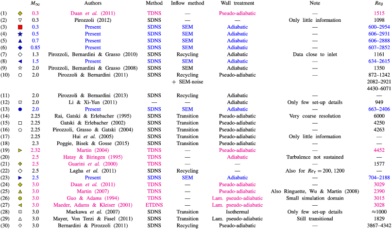
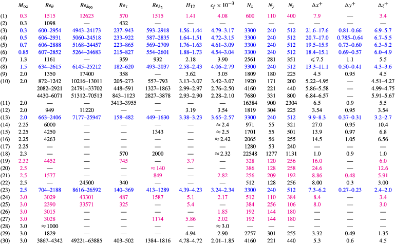
are taken into account. Both tables are an important basis for this work and will be often referred to in the following.
Summary of simulation parameters for available DNS data of CTBLs at
 $M_{\infty }\leqslant 3$
. Present DNS data are highlighted by blue colour, (E)TDNS reference data are distinguished from SDNS data by magenta colour. Additional information about the numerical set-up is given in table 2.

Summary of numerical set-up parameters for DNS data of CTBLs at
 $M_{\infty }\leqslant 3$
. Present DNS data are highlighted by blue colour, (E)TDNS reference data are distinguished from SDNS data by magenta colour. Additional information about the simulation parameters is given in table 1.

As mentioned in the introduction, many of the – essentially early – simulations suffer from simplifications concerning simulation methods or insufficient grid resolution, amongst others. These aspects play a major role in the assessment of these results, since they affect the reliability of the provided data. To assess the limitations of the summarized data, table 1 gives additional information on the simulation model, the inflow method and the wall-temperature treatment applied. If necessary, an additional note helps the integration into the overall context. Simulation models are abbreviated with (E)TDNS for an (extended, Maeder, Adams & Kleiser Reference Maeder, Adams and Kleiser2001) temporal and SDNS for a spatial model. As briefly introduced in § 1, temporal simulations suffer from the assumptions which have to be made to relate the temporal growth with the spatial boundary-layer growth as well as from the streamwise periodicity of fluctuations. Although it was shown by Martin (Reference Martin2007) by comparing SDNS and TDNS that TDNS can qualitatively reproduce the main statistics of CTBLs, differences are observable especially in the wake region of the mean-flow velocity profile. SDNS on the other hand are strongly influenced by the inflow method applied. These are distinguished in table 1 between recycling methods (Lund, Wu & Squires Reference Lund, Wu and Squires1998; Urbin & Knight Reference Urbin and Knight2001; Stolz & Adams Reference Stolz and Adams2003; Ferrante & Elghobashi Reference Ferrante and Elghobashi2004; Sagaut et al.
Reference Sagaut, Garnier, Tromeur, Larcheveque and Labourasse2004; Xu & Martin Reference Xu and Martin2004), developing turbulence by the simulation of laminar–turbulent transition by (asymmetric, subharmonic) oblique-mode breakdown (Keller & Kloker Reference Keller and Kloker2016), or synthetic eddy methods (SEM, digital filtering methods, Sandham, Yao & Lawal Reference Sandham, Yao and Lawal2003; Li & Coleman Reference Li and Coleman2004). It is worth noting that SDNS are not inevitably superior to TDNS, since inaccuracies introduced at the inlet distort the resulting flow field in excess of fifty boundary-layer thicknesses (Pirozzoli & Bernardini Reference Pirozzoli and Bernardini2011) downstream of the inlet. Only if careful inlet treatment is combined with long spatial simulation domains, can high-fidelity data be obtained. Due to its strong impact on the skin-friction coefficient
 $c_{f}$
, the respective wall-temperature boundary condition is also specified in table 1, distinguishing between an adiabatic or pseudo-adiabatic wall-temperature boundary condition. In the case of an adiabatic condition, the heat flux is suppressed in the wall-normal direction for the unsteady flow field causing temperature and Mach-number fluctuations directly at the wall (Guarini et al.
Reference Guarini, Moser, Shariff and Wray2000). These fluctuations are suppressed in the case of a pseudo-adiabatic boundary-condition, since the wall temperature (distribution) is isothermally prescribed to a theoretically derived temperature.
Table 2 summarizes the information concerning the physical and numerical set-up corresponding to the simulations referenced in table 1. Given parameters are the momentum-thickness Reynolds numbers calculated with the far-field viscosity
 $Re_{\unicode[STIX]{x1D703}}$
and the wall viscosity
 $Re_{\unicode[STIX]{x1D6FF}_{2}}$
, the boundary-layer-thickness Reynolds number
 $Re_{\unicode[STIX]{x1D6FF}_{99}}=\unicode[STIX]{x1D70C}_{e}^{\ast }u_{e}^{\ast }\unicode[STIX]{x1D6FF}_{99}^{\ast }/\unicode[STIX]{x1D707}_{e}^{\ast }$
, the skin-friction Reynolds number
 $Re_{\unicode[STIX]{x1D70F}}$
, the shape factor
 $H_{12}$
(see (5.2)), the skin-friction coefficient
 $c_{f}=2\overline{\unicode[STIX]{x1D70F}}_{w}/(\overline{\unicode[STIX]{x1D70C}}_{w}u_{e}^{2})$
with
 $\overline{\unicode[STIX]{x1D70F}}_{w}=\overline{(\unicode[STIX]{x1D707}\unicode[STIX]{x2202}u/\unicode[STIX]{x2202}y)}_{w}\approx \overline{\unicode[STIX]{x1D707}}_{w}(\unicode[STIX]{x2202}\overline{u}/\unicode[STIX]{x2202}y)_{w}$
as well as the number of grid points and the grid resolution in wall units as far as are known.
Two simulations stand out in terms of scientific acceptance. Whereas the temporal, well-resolved simulation from Guarini et al. (Reference Guarini, Moser, Shariff and Wray2000) at a free-stream Mach number of
 $M_{\infty }=2.5$
has been used as reference for a long time, the spatial simulation of Pirozzoli & Bernardini (Reference Pirozzoli and Bernardini2011) at
 $M_{\infty }=2.0$
replaced Guarini’s simulation as a new reference benchmark for CTBLs at moderate supersonic Mach numbers.
Related to the determination of compressibility effects at higher Mach numbers, the most detailed and complete work is probably given in Duan et al. (Reference Duan, Beekman and Martin2011) with a TDNS approach. Details about the underlying numerical set-up and a comparison with an SDNS reference case are given in a preceding work by Martin (Reference Martin2007).
3 Methodology and numerical set-up
In the first part of this section a brief overview of the present DNS methodology is outlined, whereas detailed information concerning the numerical set-up is given afterwards.
3.1 Methodology of the present study
The main objective of the present study is a fine-meshed analysis of CTBLs over a free-stream Mach-number range
 $0.3\leqslant M_{\infty }\leqslant 2.5$
. The use of an identical set-up for all cases allows a maximum of comparability among each other. To this end, the domain size is chosen to cover the same range of
 $\unicode[STIX]{x0394}Re_{x}=\unicode[STIX]{x1D70C}_{e}^{\ast }u_{e}^{\ast }(x_{end}^{\ast }-x_{0}^{\ast })/\unicode[STIX]{x1D707}_{e}^{\ast }$
and almost the same range of
 $Re_{\unicode[STIX]{x1D6FF}_{99}}$
for all Mach numbers on an identically spaced numerical grid in terms of
 $\unicode[STIX]{x0394}Re_{x,y,z}$
. This setting ensures the same amount and distribution of grid points at comparable boundary-layer thicknesses in terms of
 $Re_{\unicode[STIX]{x1D6FF}_{99}}$
and spatial positions in terms of
 $\unicode[STIX]{x0394}Re_{x}$
. As the result of the increased viscosity in the vicinity of the wall, however, the skin-friction Reynolds number
 $Re_{\unicode[STIX]{x1D70F}}$
is strongly decreasing for higher Mach numbers at comparable
 $Re_{\unicode[STIX]{x1D6FF}_{99}}$
, but identical
 $Re_{\unicode[STIX]{x1D70F}}$
values can be found by considering different
 $x$
-stations in the long domain. Expressed in wall units, the numerical grid shows an increasingly fine resolution for higher Mach numbers. Even if the supersonic-Mach-number simulations seem to be over-resolved, this set-up provides a maximum of comparability, since turbulent structures in the wake region of the TBL are resolved with an identically spaced grid.
The length of the simulation domain is chosen to cover a Reynolds numbers range
 $300\lesssim Re_{\unicode[STIX]{x1D703}}\lesssim 3000$
for the nearly incompressible reference case at
 $M_{\infty }=0.3$
. The presented data provide a meaningful contribution even to the incompressible data-base (Schlatter & Örlü Reference Schlatter and Örlü2010:
 $Re_{\unicode[STIX]{x1D703},max}\approx 4300$
). All grid data are summarized in table 2 next to their compressible counterparts and explained in more detail in § 3.4, after providing a basic explanation of the numerical set-up.
3.2 Numerical method
All computations are performed with the compressible high-order in-house DNS code
 $NS3D$
, which has been extensively validated for a broad variety of applications. Fundamentals of the code are described in Linn & Kloker (Reference Linn, Kloker and Gülhan2008, Reference Linn and Kloker2011), Babucke (Reference Babucke2009) and Keller & Kloker (Reference Keller and Kloker2014, Reference Keller and Kloker2016). It solves the three-dimensional, unsteady, compressible Navier–Stokes equations together with the continuity and energy equation in conservative formulation and Laplace formulation of the viscous terms. With the velocity vector
 $\boldsymbol{u}=[u,v,w]^{\text{T}}$
with components in streamwise, wall-normal and spanwise directions
 $x$
,
 $y$
and
 $z$
, the dimensionless solution vector is
 $\boldsymbol{Q}=[\unicode[STIX]{x1D70C},\unicode[STIX]{x1D70C}u,\unicode[STIX]{x1D70C}v,\unicode[STIX]{x1D70C}w,E]^{\text{T}}$
, where
 $\unicode[STIX]{x1D70C}$
and
 $E$
are the density and the total energy, respectively. Velocities and length scales are normalized by the streamwise reference velocity
 $u_{\infty }^{\ast }$
and the reference length
 $L^{\ast }=\unicode[STIX]{x1D6FF}_{99,0}$
, respectively. Thermodynamical quantities are normalized with the reference temperature
 $T_{\infty }^{\ast }$
and the reference density
 $\unicode[STIX]{x1D70C}_{\infty }^{\ast }$
; the pressure
 $p$
is non-dimensionalized by
 $\unicode[STIX]{x1D70C}_{\infty }^{\ast }u_{\infty }^{\ast 2}$
. The specific heats
 $c_{p}$
and
 $c_{v}$
as well as the Prandtl number
 $Pr$
are assumed to be constant. The temperature dependence of the viscosity is modelled by Sutherland’s law. The equations are solved on a block-structured Cartesian grid spanning a rectangular integration domain.
The chordwise and wall-normal directions are discretized using sixth-order subdomain-compact finite differences (Keller & Kloker Reference Keller and Kloker2013). In the periodic spanwise
 $z$
-direction the derivatives are calculated by a Fourier-spectral ansatz. The classical fourth-order Runge–Kutta scheme is used for time integration.
3.3 Numerical set-up and boundary conditions
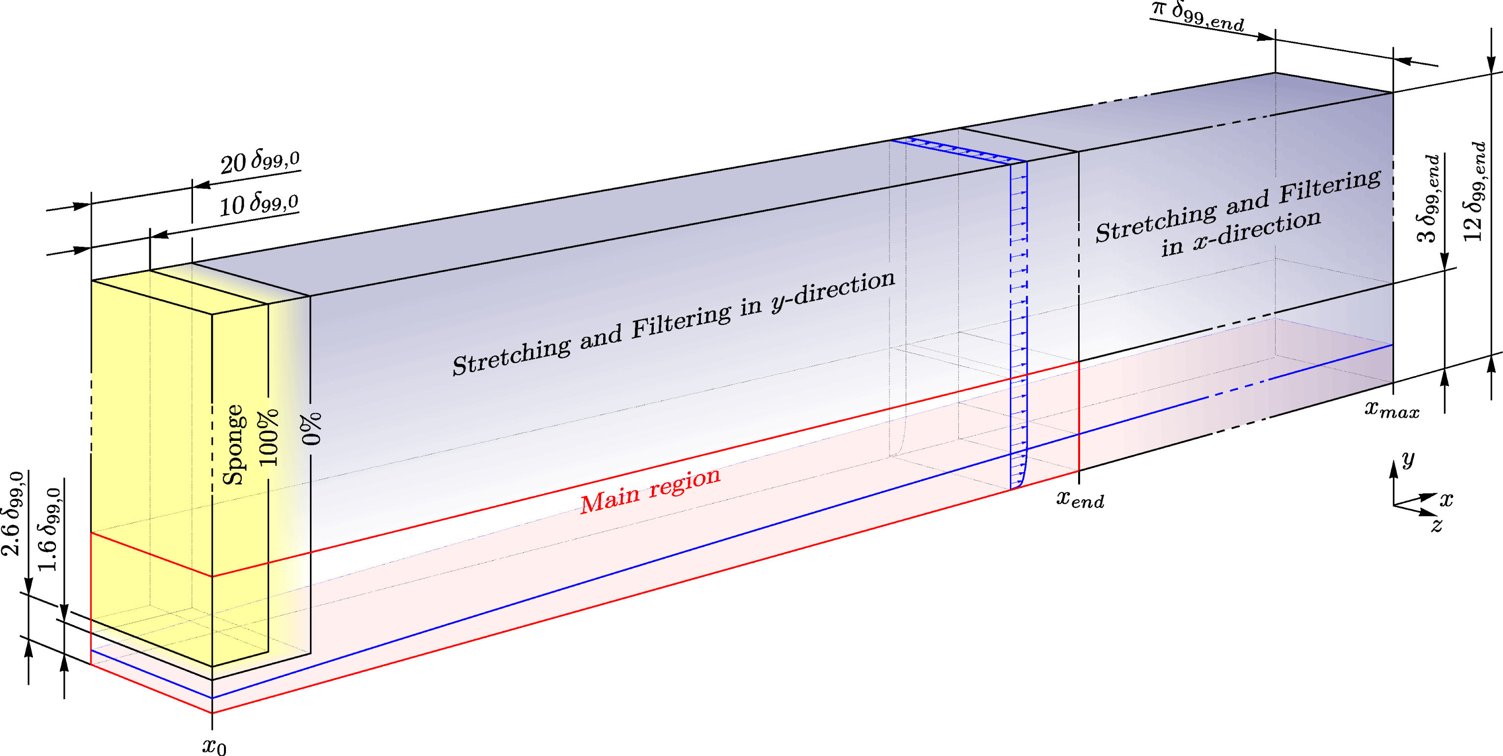
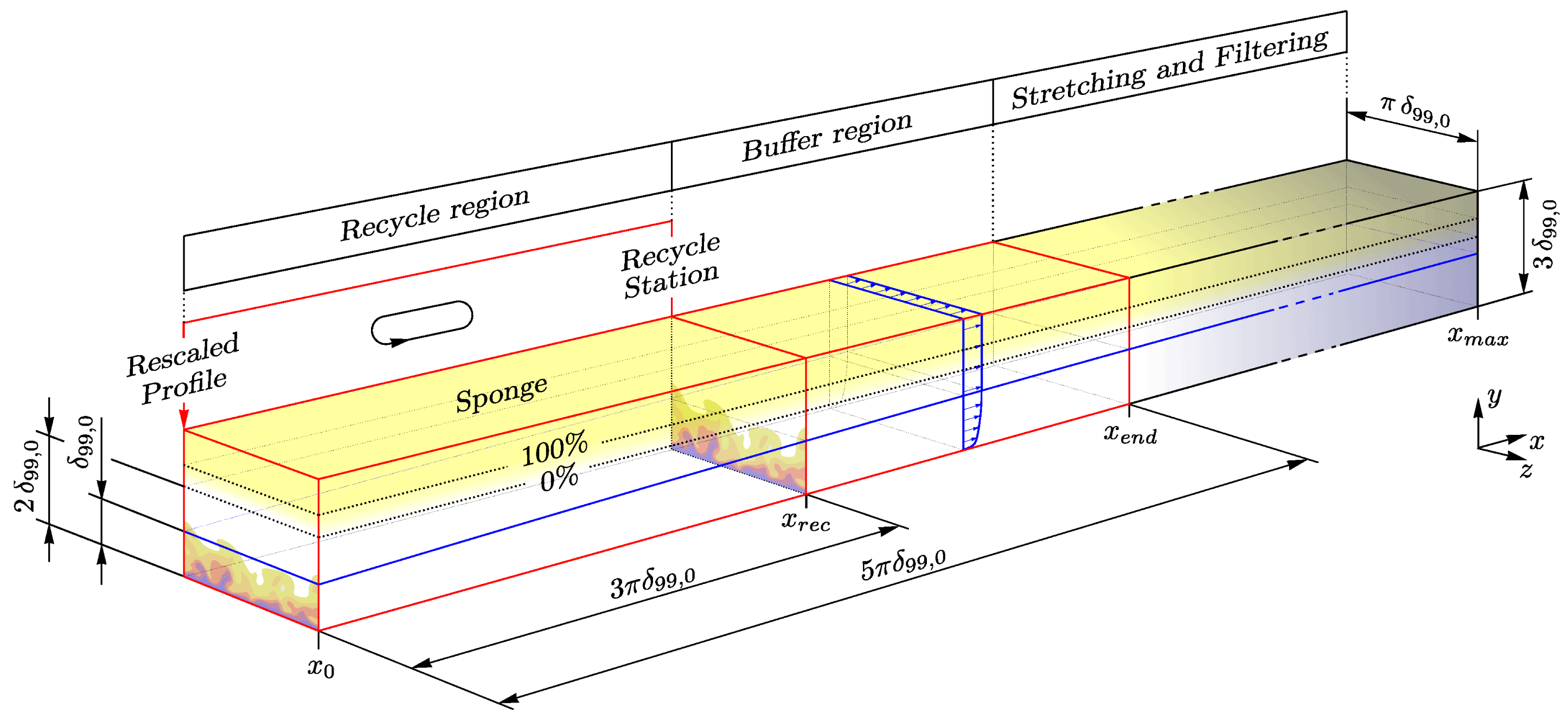
Simulation domain for the present DNS. The yellow coloured region represents a sponge zone, blue coloured regions represent grid-stretched and spatially filtered regions. The red bordered zone represents the main region of the simulation.

A sketch of the simulation domain is presented in figure 1. Analogous to simulations available in the literature, the main region of the simulation domain is designed with a height of at least three boundary-layer thicknesses
 $\unicode[STIX]{x1D6FF}_{99,end}$
, measured at the end of the main region
 $x_{end}$
. Due to the spanwise Fourier-spectral ansatz, the spanwise dimension is set to
 $\unicode[STIX]{x03C0}\,\unicode[STIX]{x1D6FF}_{99,end}$
.
At the solid wall, the flow field is treated as fully adiabatic with
 $(\text{d}T/\text{d}y)_{w}=0$
which suppresses any heat exchange between wall and fluid, whereas the pressure at the wall is calculated by
 $(\text{d}p/\text{d}y)_{w}=0$
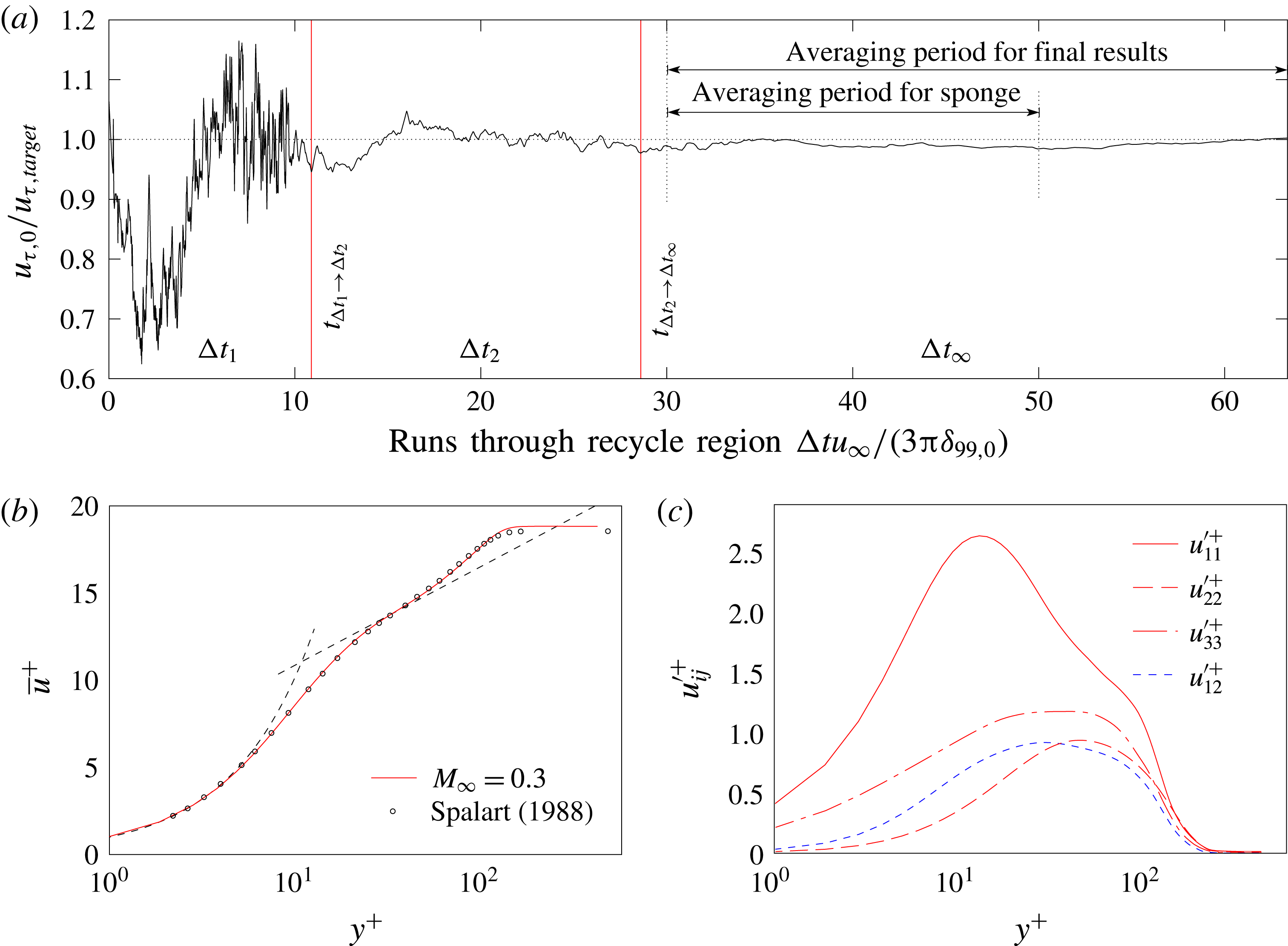
. For the velocity components, the no-slip impermeable wall boundary condition is applied. At the inlet a digital filtering SEM approach is used to generate an unsteady, turbulent inflow condition (basics of the code can be found in Touber (Reference Touber2010), additional information is given in e.g. Klein, Sadiki & Janicka (Reference Klein, Sadiki and Janicka2003), Touber & Sandham (Reference Touber and Sandham2011) and Kim, Castro & Xie (Reference Kim, Castro and Xie2013)). The required distributions for the mean-velocity field and for the Reynolds fluctuations are extracted from a small auxiliary simulation using a recycling method, see appendix A. Even if the SEM boundary condition provides a pseudo-physical turbulent flow field at the inlet of the domain, an induction distance is needed until fully developed turbulence is established in which the boundary layer reaches an equilibrium state with the local production and dissipation of turbulent kinetic energy balancing each other (Schlatter et al.
Reference Schlatter, Örlü, Li, Brethouwer, Fransson, Johansson, Alfredsson and Henningson2009). According to Schlatter et al. (Reference Schlatter, Örlü, Li, Brethouwer, Fransson, Johansson, Alfredsson and Henningson2009), the induction distance can be estimated by considering the von Kármán integral equation relating the local skin friction
 $c_{f}$
to the growth of the momentum thickness
 $\unicode[STIX]{x1D703}$
(
 $c_{f}=2\text{d}\unicode[STIX]{x1D703}/\text{d}x$
), if fluctuation and pressure terms are neglected (von Kármán Reference von Kármán1921; Pohlhausen Reference Pohlhausen1921). Based on this argument, the induction distance of the
 $M_{\infty }=0.3$
case may be defined to be about
 $28\unicode[STIX]{x1D6FF}_{99,0}$
initial boundary layer thicknesses, corresponding to 6 % of the main region of the computational domain. Due to the decreasing skin-friction Reynolds number
 $Re_{\unicode[STIX]{x1D70F}}$
for higher Mach-number cases, the flow becomes more stable at the wall and the induction distance elongates up to
 $85\unicode[STIX]{x1D6FF}_{99,0}$
for the
 $M_{\infty }=2.5$
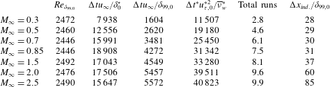
case, corresponding to 18 % of the main region of the computational domain. A summary of all induction distances for the different Mach number cases is given in table 3. In order to prevent the included far-field flow from being unduly distorted by the transient process, a sponge region as described in Kurz & Kloker (Reference Kurz and Kloker2014) and Schmidt (Reference Schmidt2014) is placed in the inlet region of the simulation set-up outside the boundary layer, damping the flow to unperturbed, prescribed far-field values. At the outflow itself, the time derivative, respectively the complete space operator, is extrapolated with
 $\unicode[STIX]{x2202}\boldsymbol{Q}/\unicode[STIX]{x2202}t|_{N}=\unicode[STIX]{x2202}\boldsymbol{Q}/\unicode[STIX]{x2202}t|_{N-1}$
; for both
 $n=N-1$
and
 $N$
all second
 $x$
-derivatives are neglected, and biased difference stencils are used for the first derivatives. For subsonic flows,
 $\unicode[STIX]{x1D70C}$
,
 $T$
, and
 $p$
are kept constant at the top of the domain. The velocity components
 $u$
and
 $w$
are specified by
 $\text{d}/\text{d}y=0$
, whereas the wall-normal velocity component
 $v$
is calculated from the continuity equation under the assumption of
 $\text{d}\unicode[STIX]{x1D70C}/\text{d}y=0$
such that
 $\text{d}v/\text{d}y=-1/\unicode[STIX]{x1D70C}\,(\text{d}(\unicode[STIX]{x1D70C}u)/\text{d}x+\text{d}(\unicode[STIX]{x1D70C}w)/\text{d}z)$
. For supersonic flows, all flow variables are computed such that the gradient along spatial characteristics is zero, except for the pressure, which is derived from the equation of state. In both wall-normal and streamwise directions, exponential grid stretching is applied to the numerical grid, and tenth-order implicit filtering is applied in order to avoid reflections from the boundaries (Colonius, Lele & Moin Reference Colonius, Lele and Moin1993; Visbal & Gaitonde Reference Visbal and Gaitonde2002).
3.4 Simulation parameters
The main region of the computational box has a dimension of
 $42\,\unicode[STIX]{x1D6FF}_{99,end}\times 3\,\unicode[STIX]{x1D6FF}_{99,end}\times \unicode[STIX]{x03C0}\,\unicode[STIX]{x1D6FF}_{99,end}$
in the streamwise, wall-normal and spanwise direction, respectively. Based on the simulations provided by Schlatter & Örlü (Reference Schlatter and Örlü2010), Pirozzoli & Bernardini (Reference Pirozzoli and Bernardini2011) and investigations about a minimum domain width provided by Poggie, Bisek & Gosse (Reference Poggie, Bisek and Gosse2015) (see also Agostini et al.
Reference Agostini, Leschziner, Poggie, Bisek and Gaitonde2017), a domain width of
 $\unicode[STIX]{x03C0}\unicode[STIX]{x1D6FF}_{99,max}$
is sufficiently large to avoid coherent dynamics resulting from the finite span. The grid is based on the most restricting, nearly incompressible case at
 $M_{\infty }=0.3$
. It is chosen to be in-between the benchmark DNS by Schlatter et al. (Reference Schlatter, Örlü, Li, Brethouwer, Fransson, Johansson, Alfredsson and Henningson2009) and Schlatter & Örlü (Reference Schlatter and Örlü2010). The grid size is
 $3100\times 205\times 512$
for the main region and
 $3300\times 240\times 512$
for the overall domain. Calculated in wall units, this gives a grid spacing of
 $\unicode[STIX]{x0394}x^{+}=21$
,
 $\unicode[STIX]{x0394}y_{1}^{+}=0.8$
and
 $\unicode[STIX]{x0394}z^{+}=6.8$
at
 $Re_{\unicode[STIX]{x1D703}}=670$
for
 $M_{\infty }=0.3$
in the three dimensions. To ensure adequate grid resolution, grid convergence studies have been performed for the most restricting case at
 $M_{\infty }=0.3$
in a simulation domain which has been reduced in all three spatial directions, spanning a final Reynolds-number range of
 $300\lesssim Re_{\unicode[STIX]{x1D703}}\lesssim 1400$
. Grid convergence has been ensured by evaluation of the fluctuating wall shear stress
 $\unicode[STIX]{x1D70F}_{w}^{\prime +}=\lim _{y^{+}\rightarrow 0}\sqrt{\overline{u^{\prime }u^{\prime }}}^{+}/\overline{u}^{+}$
(Alfredsson et al.
Reference Alfredsson, Johansson, Haritonidis and Eckelmann1988) and the energy spectra. Details about the reduced grid are given in Wenzel et al. (Reference Wenzel, Selent, Kloker and Rist2017). The grid parameters and important Reynolds numbers for the fully developed region of all simulations presented here are summarized in table 2 next to data from the literature. The basic thermodynamic flow parameters like the far-field temperature
 $T_{\infty }^{\ast }=288.15~\text{K}$
, far-field density
 $\unicode[STIX]{x1D70C}_{\infty }^{\ast }=1.225~\text{kg}~\text{m}^{-3}$
, Prandtl number
 $Pr=0.71$
, specific gas constant
 $R^{\ast }=287~\text{J}~(\text{kg}~\text{K})^{-1}$
and ratio of specific heats
 $\unicode[STIX]{x1D6FE}=1.4$
are set equal for all cases.
Data averaging is performed over both time and spanwise direction and does not start before the flow has passed the whole domain at least twice. An overview of the time-averaging used for different Mach numbers is given in table 3. Whereas unsteady variables are denoted by the use of small letters
 $f$
, time- and space-averaged values are denoted by an overbar
 $\overline{f}$
and fluctuating components by a prime
 $f^{\prime }$
, leading to
 $f=\overline{f}+f^{\prime }$
.
Summary of time-averaging parameters with the boundary-layer Reynolds number
 $Re_{\unicode[STIX]{x1D6FF}_{99,0}}$
measured at the inlet and the time-averaging period
 $\unicode[STIX]{x0394}t$
:
 $\unicode[STIX]{x0394}tu_{\infty }/\unicode[STIX]{x1D6FF}_{0}^{\star }$
and
 $\unicode[STIX]{x0394}tu_{\infty }/\unicode[STIX]{x1D6FF}_{99,0}$
give the amount of boundary-layer thicknesses
 $\unicode[STIX]{x1D6FF}_{99,0}$
and displacement thicknesses
 $\unicode[STIX]{x1D6FF}_{0}^{\star }$
, which have flowed through during
 $\unicode[STIX]{x0394}t$
at the inlet of the domain;
 $\unicode[STIX]{x0394}t^{\ast }u_{\unicode[STIX]{x1D70F},0}^{\ast 2}/\overline{\unicode[STIX]{x1D708}}_{w}^{\ast }$
represents
 $\unicode[STIX]{x0394}t$
in wall units
 $\unicode[STIX]{x0394}t^{+}$
. The number of total runs gives the amount of time-averaged runs through the main region.
 $\unicode[STIX]{x0394}x_{ind.}/\unicode[STIX]{x1D6FF}_{99,0}$
gives the induction distance which is needed to reach an equilibrium state.

3.5 Calculation of boundary-layer properties
For compressible flows, many boundary-layer quantities are highly sensitive to their underlying definitions. Especially for the calculation of
 $Re_{\unicode[STIX]{x1D70F}}$
and its importance for compressible scaling laws, the weakly defined boundary-layer thickness
 $\unicode[STIX]{x1D6FF}_{99}$
has a significant influence by defining the state of the boundary layer. In our study, the boundary-layer edge (index
 $e$
) is determined at the wall-normal position where the wall-normal gradient
 $\text{d}\breve{u}/\text{d}y$
(or the spanwise vorticity
 $\unicode[STIX]{x1D714}_{z}$
directly) of the pseudo-velocity field
 $\breve{u}(x,y)=-\int _{0}^{y}\unicode[STIX]{x1D714}_{z}(x,y)\,\text{d}y$
with
 $\unicode[STIX]{x1D714}_{z}=-\unicode[STIX]{x2202}\overline{u}/\unicode[STIX]{x2202}y+\unicode[STIX]{x2202}\overline{v}/\unicode[STIX]{x2202}x$
drops below
 $10^{-6}$
of
 $\text{d}\breve{u}/\text{d}y$
at the wall (Spalart & Strelets Reference Spalart and Strelets2000). All boundary-layer edge quantities are evaluated at this position (index
 $e$
). The boundary-layer thickness
 $\unicode[STIX]{x1D6FF}_{99}$
is determined where the streamwise velocity
 $\overline{u}$
reaches 99 % of
 $u_{e}$
. It has been ensured that all boundary-layer edge values are sufficiently distant from the temperature boundary-layer thickness
 $\unicode[STIX]{x1D6FF}_{T,99}$
, thereby allowing the value of the far-field viscosity
 $\unicode[STIX]{x1D708}_{e}$
in particular not to be affected by the temperature distribution inside the temperature boundary layer. The displacement thickness, the momentum thickness and the shape factor are:
 $$\begin{eqnarray}\displaystyle & \displaystyle \unicode[STIX]{x1D6FF}^{\star }=\int _{0}^{\unicode[STIX]{x1D6FF}_{99}}\left(1-\frac{\overline{\unicode[STIX]{x1D70C}}\,\overline{u}}{\unicode[STIX]{x1D70C}_{e}u_{e}}\right)\text{d}y, & \displaystyle\end{eqnarray}$$
 $$\begin{eqnarray}\displaystyle & \displaystyle \unicode[STIX]{x1D703}=\int _{0}^{\unicode[STIX]{x1D6FF}_{99}}\frac{\overline{\unicode[STIX]{x1D70C}}\,\overline{u}}{\unicode[STIX]{x1D70C}_{e}u_{e}}\left(1-\frac{\overline{u}}{u_{e}}\right)\text{d}y, & \displaystyle\end{eqnarray}$$
 $$\begin{eqnarray}\displaystyle & \displaystyle H_{12}=\frac{\unicode[STIX]{x1D6FF}^{\star }}{\unicode[STIX]{x1D703}}. & \displaystyle\end{eqnarray}$$
It should be noted that this definition is different to the one used by Pirozzoli & Bernardini (Reference Pirozzoli and Bernardini2011) for instance, who do not discern between the boundary-layer edge
 $\unicode[STIX]{x1D6FF}_{e}$
and boundary-layer thickness
 $\unicode[STIX]{x1D6FF}_{99}$
. However, it will be shown that our definition more closely matches the incompressible reference data for the shape factor, since most of the existing data were also obtained by distinguishing between far-field and boundary-layer-edge values. Both methods will be compared for the example of the
 $M_{\infty }=2.0$
case in the discussion of the shape factor distributions in § 4.
3.6 Validation of the adiabatic boundary condition
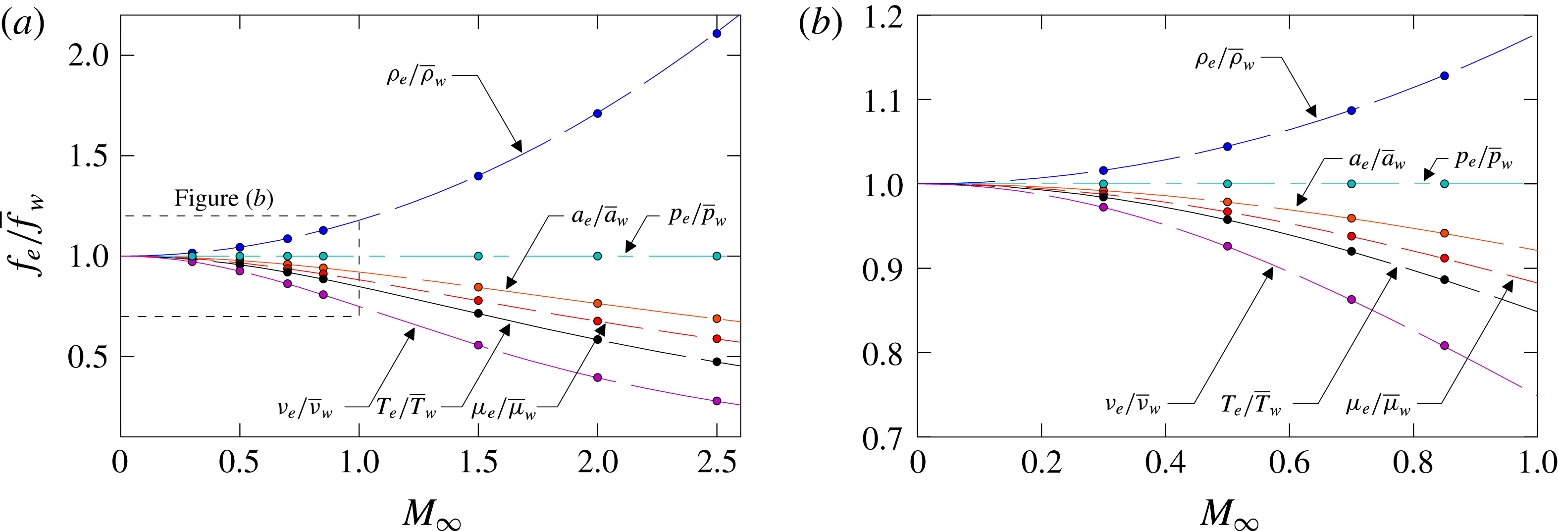
Especially for compressible scaling laws the flow parameters at the wall play a major role. An overview of the simulated edge-to-wall ratios is given in figure 2. Whereas the plotted lines represent the theoretical behaviour of the given parameters, the coloured dots show the simulation results which are constant over the whole simulation domain behind the initial transition region. The adiabatic wall temperature
 $\overline{T}_{aw}$
is given by
 $$\begin{eqnarray}\frac{\overline{T}_{aw}}{T_{e}}=1+r\frac{\unicode[STIX]{x1D6FE}-1}{2}M_{\infty }^{2},\end{eqnarray}$$
with the recovery factor
 $r=Pr^{1/3}$
. The resulting values for the speed of sound, wall density (with
 $p_{e}=\overline{p}_{w}$
, see figure 18 in the appendix) and viscosity are given by
 $$\begin{eqnarray}\overline{a}_{w}=\sqrt{\frac{\overline{T}_{aw}}{M_{\infty }^{2}}},\quad \overline{\unicode[STIX]{x1D70C}}_{w}=\frac{p_{e}\unicode[STIX]{x1D6FE}M_{\infty }^{2}}{\overline{T}_{aw}},\end{eqnarray}$$
 $$\begin{eqnarray}\overline{\unicode[STIX]{x1D707}}_{w}=(\overline{T}_{aw})^{3/2}\left(\frac{1+S_{1}}{\overline{T}_{aw}+S_{1}}\right),\quad S_{1}=\frac{110.4K}{T_{\infty }^{\ast }}.\end{eqnarray}$$
All simulated edge-to-wall ratios for the given parameters show a nearly perfect agreement with their theoretical (partly empirical) predictions. This good agreement means that using adiabatic wall boundary conditions (as in the present DNS) leads to the same theoretical mean-flow quantities at the wall as if the pseudo-adiabatic condition were used. Thus, the temperature mean value does not depend on allowing or suppressing wall-temperature fluctuations, and differences in the streamwise evolution of mean-flow quantities like
 $c_{f}$
for instance are not expected to be observed. How far other fluctuations are affected by the type of the temperature boundary condition will be discussed below.
Comparison of various edge-to-wall ratios
 $f_{e}/\overline{f}_{w}$
compared to theoretical predictions for all simulated Mach numbers
 $M_{\infty }$
(a) and close-up for
 $M_{\infty }<1$
(b). Simulation results are represented by filled circles and theoretical predictions are given as dashed lines.

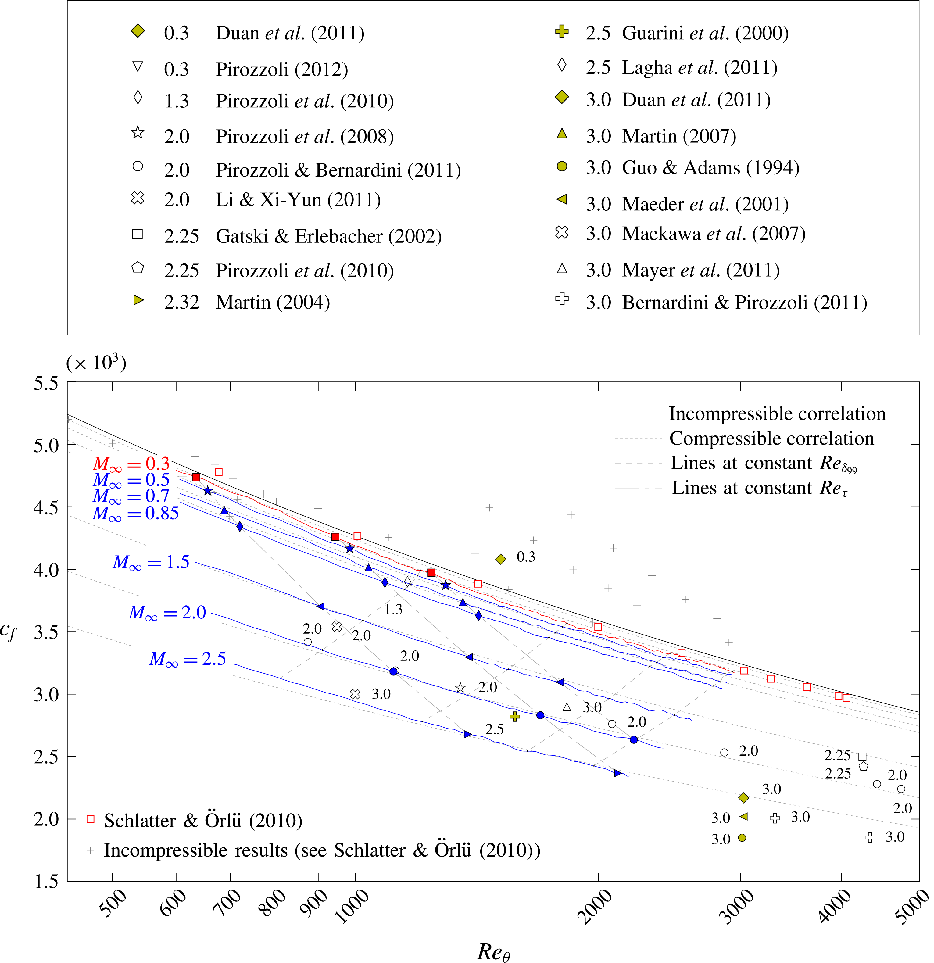
Skin-friction coefficient
 $c_{f}$
as a function of
 $Re_{\unicode[STIX]{x1D703}}$
(cf. Schlatter & Örlü Reference Schlatter and Örlü2010). The incompressible correlation is given by
 $c_{f}=0.024\,Re_{\unicode[STIX]{x1D703}}^{-1/4}$
(Smits, Matheson & Joubert Reference Smits, Matheson and Joubert1983), the compressible one by (4.1). A detailed legend of all presented results is given in table 1.

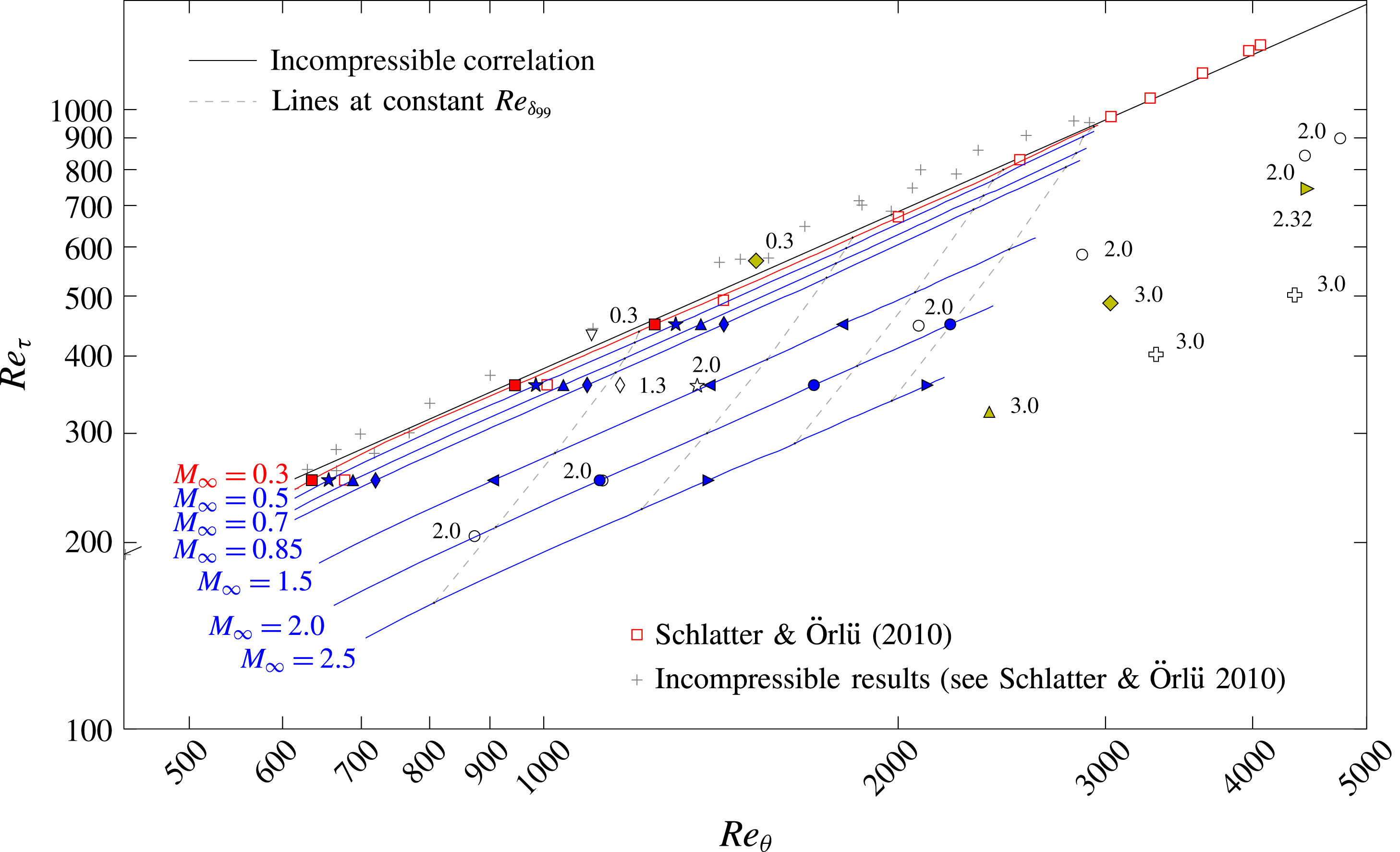
Skin-friction-velocity Reynolds number
 $Re_{\unicode[STIX]{x1D70F}}$
as a function of
 $Re_{\unicode[STIX]{x1D703}}$
(cf. Schlatter & Örlü Reference Schlatter and Örlü2010). The incompressible correlation is given by
 $Re_{\unicode[STIX]{x1D70F}}=1.13\,Re_{\unicode[STIX]{x1D703}}^{0.843}$
(Schlatter & Örlü Reference Schlatter and Örlü2010). A detailed legend of all presented results is given in table 1 or figure 3.

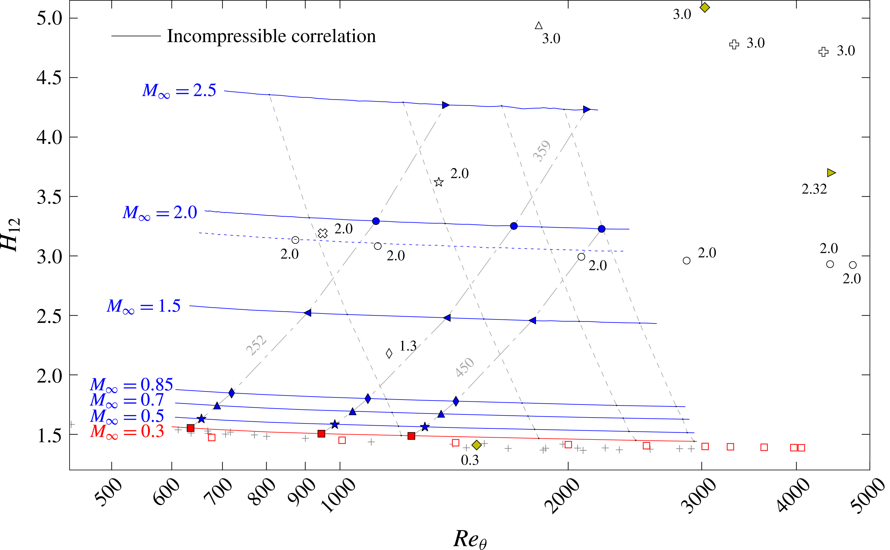
Shape factor
 $H_{12}$
as a function of
 $Re_{\unicode[STIX]{x1D703}}$
(cf. Schlatter & Örlü Reference Schlatter and Örlü2010). The incompressible correlation is given as the shape of the integrated incompressible composite profiles (Chauhan, Monkewitz & Nagib Reference Chauhan, Monkewitz and Nagib2009). The dashed blue line gives the shape factor
 $H_{12}$
, calculated by the method described in Pirozzoli & Bernardini (Reference Pirozzoli and Bernardini2011) for the
 $M_{\infty }=2.0$
case. A complete legend is given in figures 3 and 4 and table 1.

4 Spatial evolution of averaged flow statistics
This section focuses on the quantification of Mach-number effects on substantial mean values of CTBLs. Therefore, the turbulence statistics collected by Schlatter & Örlü (Reference Schlatter and Örlü2010) for incompressible TBLs are extended to the compressible regime with the present DNS data and DNS data available in the literature (tables 1 and 2). Even though only Schlatter & Örlü’s simulation will be used as incompressible reference for the present results in the following (▫ (red) in figures 3–6), other incompressible data are also given as they provide an impression of DNS-data scattering in the incompressible regime. Since they do not contribute to the overall context however, they are represented by grey-coloured plus symbols (
 $+$
) without being specifically labelled and distinguished. A detailed specification of these data can be found in Schlatter & Örlü (Reference Schlatter and Örlü2010). The streamwise evolution of our results is represented by red lines for the nearly incompressible simulation at
 $M_{\infty }=0.3$
and by blue lines for the higher-Mach-number cases. Positions where local flow-field data are extracted for the following investigations are represented by red filled squares for the nearly incompressible case at
 $M_{\infty }=0.3$
(▪) and by blue filled symbols for higher Mach numbers (
 $\star$
, ▴, ♦, ◂, ●, ▸). For all figures given in this section, compressible literature reference data are distinguished by yellow filled symbols for TDNS (♦, ▸,


 $\unicode[STIX]{x2B20}$
, ▵,

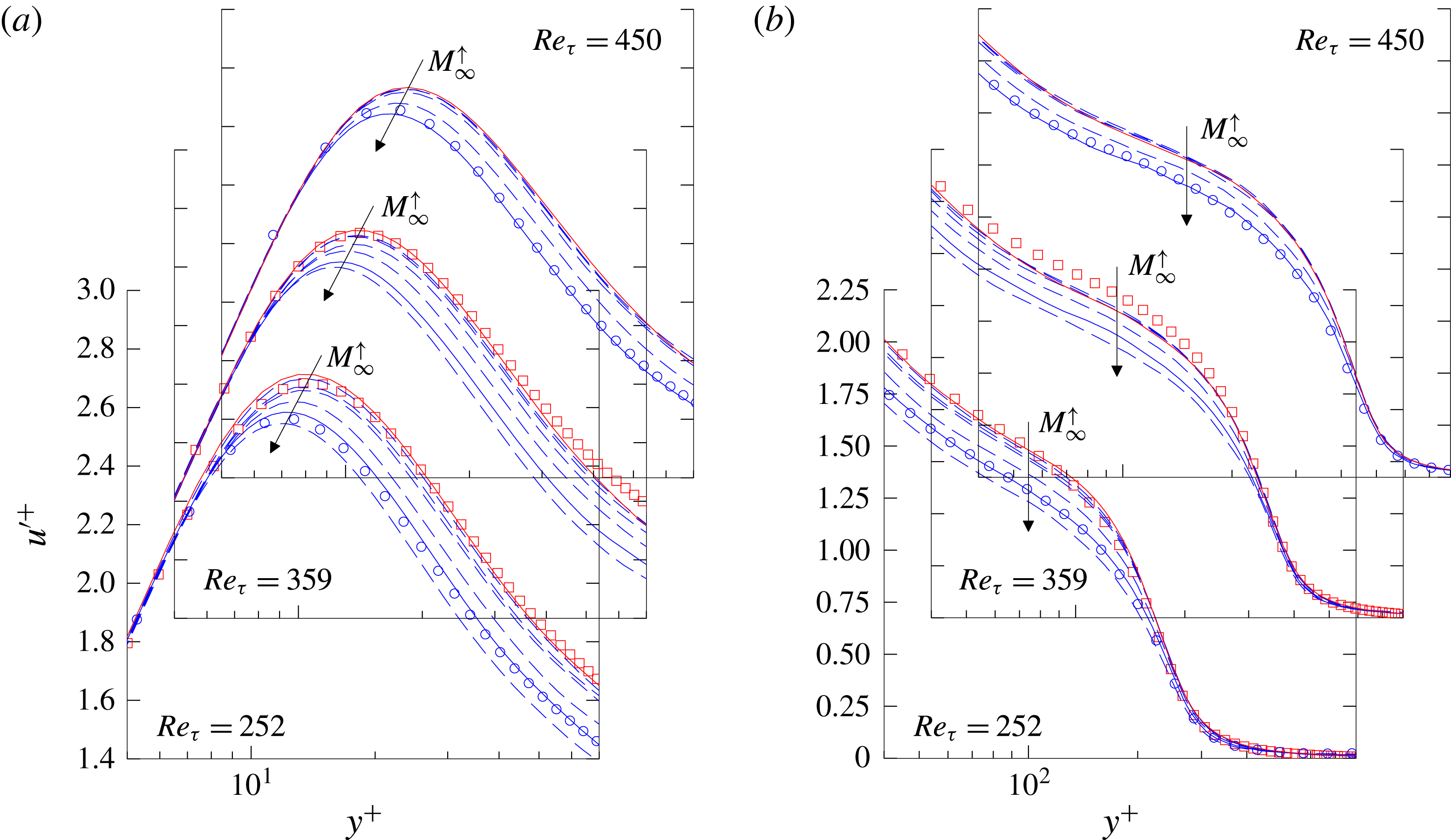
Near-wall behaviour of the streamwise velocity fluctuation
 $u^{\prime +}=\sqrt{\overline{u^{\prime }u^{\prime }}}/u_{\unicode[STIX]{x1D70F}}$
in inner scaling over
 $Re_{\unicode[STIX]{x1D70F}}$
(cf. Schlatter & Örlü Reference Schlatter and Örlü2010). (a) Value of
 $u_{max}^{\prime +}$
and (b) wall-normal position of maximum
 $y^{+}(u_{max}^{\prime +})$
, compared to incompressible DNS by Schlatter & Örlü (Reference Schlatter and Örlü2010) (▫ (red)), compressible at
 $M_{\infty }=2.0$
by Pirozzoli & Bernardini (Reference Pirozzoli and Bernardini2011) (○) and
 $M_{\infty }=3.0$
by Bernardini & Pirozzoli (Reference Bernardini and Pirozzoli2011) (

 $f(Re_{\unicode[STIX]{x1D70F}})=a+m\ln Re_{\unicode[STIX]{x1D70F}}$
.

4.1 Spatial evolution of mean flow statistics
Figures 3–5 give the skin-friction coefficient
 $c_{f}$
, the skin-friction-velocity Reynolds number
 $Re_{\unicode[STIX]{x1D70F}}$
and the shape factor
 $H_{12}$
, respectively, as functions of
 $Re_{\unicode[STIX]{x1D703}}$
. With the objective of linking the various Mach-number cases, isolines are plotted for positions of the same
 $Re_{\unicode[STIX]{x1D6FF}_{99}}$
and
 $Re_{\unicode[STIX]{x1D70F}}$
, additionally. The plot for the
 $c_{f}$
-distribution (figure 3) is supplemented by an incompressible correlation (black solid line) based on the
 $1/7$
-power law of the form
 $c_{f}=0.024\,Re_{\unicode[STIX]{x1D703}}^{-1/4}$
(Smits et al.
Reference Smits, Matheson and Joubert1983) together with its compressibility-transformed counterparts (grey short-dashed lines). These are calculated with the ‘most popular and best of its type ever developed’ (White Reference White2006) theoretically derived compressibility transformation (Van Driest Reference Van Driest1956) which was verified among others by Hopkins & Inouye (Reference Hopkins and Inouye1971) for experiments, Pirozzoli & Bernardini (Reference Pirozzoli and Bernardini2011) for SDNS and Duan et al. (Reference Duan, Beekman and Martin2011) for TDNS. The theoretical curve can be physically interpreted as an incompressible
 $c_{f}$
-distribution which is stretched by compressibility and viscosity effects (White Reference White2006). If the subscripts
 $inc$
and
 $c$
stand for incompressible and compressible values, respectively, it can be written as
 $$\begin{eqnarray}c_{f,c}=\frac{1}{F_{c}}c_{f,inc}\left(\frac{\unicode[STIX]{x1D707}_{e}}{\overline{\unicode[STIX]{x1D707}}_{w}}Re_{\unicode[STIX]{x1D703},c}\right).\end{eqnarray}$$
In the adiabatic case,
 $$\begin{eqnarray}F_{c}=\frac{\overline{T}_{aw}/T_{e}-1}{\sin ^{-1}A},\quad A=\frac{\overline{T}_{aw}/T_{e}-1}{\sqrt{\overline{T}_{aw}/T_{e}(\overline{T}_{aw}/T_{e}-1)}}.\end{eqnarray}$$
The plot for the
 $Re_{\unicode[STIX]{x1D70F}}$
-distribution (figure 4) is supplemented by an incompressible best-fit power-law relation provided by Schlatter & Örlü (Reference Schlatter and Örlü2010) with
 $Re_{\unicode[STIX]{x1D70F}}=1.13\,Re_{\unicode[STIX]{x1D703}}^{0.843}$
, whereas the shape factor distribution
 $H_{12}$
(figure 5) is supplemented by the shape of integrated incompressible composite profiles (Chauhan et al.
Reference Chauhan, Monkewitz and Nagib2009).
First, only the results for the nearly incompressible case at
 $M_{\infty }=0.3$
should be considered for figures 3–5 simultaneously (red solid lines marked with ▪ (red)). Compressibility effects are not absent in this case, since the temperature differs up to 2 % in the wall region from its incompressible counterpart, see figure 2(b). Nevertheless, the result for the skin-friction coefficient
 $c_{f}$
in figure 3 is in good agreement with the most reliable incompressible DNS data provided by Schlatter & Örlü (Reference Schlatter and Örlü2010) (▫ (red)) and the given incompressible correlation (black solid line). Comparing the curve for
 $Re_{\unicode[STIX]{x1D70F}}$
to the incompressible references in figure 4, a nearly perfect fit can be determined with the best-fit regression (black solid line), whereas differences can be observed between the
 $M_{\infty }=0.3$
case (▪ (red)) and Schlatter & Örlü’s data (▫ (red)) for lower Reynolds numbers. Since these differences disappear for higher Reynolds numbers, they can be traced back to history effects caused by the different inflow boundary conditions which are applied in both simulations. Due to its dependence on sensitive parameters like the boundary-layer thickness
 $\unicode[STIX]{x1D6FF}_{99}$
and the skin-friction velocity
 $u_{\unicode[STIX]{x1D70F}}$
on the ordinate as well as the momentum thickness
 $\unicode[STIX]{x1D703}$
on the abscissa, figure 4 provides an honest measure for the data quality. The shape factor
 $H_{12}$
of our
 $M_{\infty }=0.3$
case, given in figure 5, shows a systematic difference to the incompressible results by about 2 %. Since the incompressible correlation and the
 $M_{\infty }=0.3$
case collapse when the shape factor is calculated with its incompressible formulation by neglecting the density variations across the boundary layer (see Wenzel et al.
Reference Wenzel, Selent, Kloker and Rist2017), this difference can be traced back to compressibility effects. Therefore, the
 $M_{\infty }=0.3$
case can be used as a trusted incompressible reference for the quantification of compressibility effects in the following.
Comparing the
 $c_{f}$
-distributions of the compressible results (blue marked solid lines) with the grey short-dashed lines in figure 3 first, representing the compressibility transformed
 $c_{f}$
-distributions of the incompressible correlation (see (4.1)), a systematic shift can be observed for higher Reynolds numbers at low Mach numbers. This shift virtually vanishes for increasing Mach numbers. Taking into account that this shift is caused by a mismatch between the incompressible correlation and the
 $M_{\infty }=0.3$
case, the compressibility effect on the
 $c_{f}$
-distribution is slightly underpredicted by Van Driest’s flat-plate theory for
 $M_{\infty }=2.5$
. If the literature data-base for compressible DNS is assessed for mainly supersonic flows (♦,


 $\unicode[STIX]{x2B20}$
,

 $M_{\infty }=2.0$
(○, ✩) can provide a comparable accuracy. Whereas an adiabatic boundary-condition is applied for the former, a pseudo-adiabatic one is applied for the latter, see table 1. Taking into account that the TDNS results by Guo & Adams (Reference Guo and Adams1994) and Maeder et al. (Reference Maeder, Adams and Kleiser2001) for
 $M_{\infty }=3.0$
(●, ◂ (yellow)) are obtained with prescribing the laminar adiabatic wall temperature (corresponding to a cooled wall), all other TDNS results (♦,

 $c_{f}$
-values being about 5 %–10 % too high. If particular attention is paid to our subsonic results, differences of up to 5 % can be observed between the
 $M_{\infty }=0.3$
(▪ (red)) and the
 $M_{\infty }=0.85$
case (♦ (blue)). Even if these differences are clearly quantifiable for the present simulations, it should be noted that all subsonic results lie in between the scattering of incompressible DNS data (
 $+$
). Consequently, it is advisable to simulate an independent incompressible reference case with a comparable set-up, if compressibility effects are to be quantified in the subsonic Mach-number-range.
The distributions of the skin-friction Reynolds number
 $Re_{\unicode[STIX]{x1D70F}}$
for the compressible results in figure 4 give almost parallel curves to the incompressible results. Again, the agreement with the data from Pirozzoli & Bernardini (Reference Pirozzoli and Bernardini2011) (○) for the
 $M_{\infty }=2.0$
case (● (blue)) should be underlined. However, whereas their first simulation (
 $872\leqslant Re_{\unicode[STIX]{x1D703}}\leqslant 1242$
) is in complete agreement with our data, their second (
 $2082\leqslant Re_{\unicode[STIX]{x1D703}}\leqslant 2921$
) and third (
 $4430\leqslant Re_{\unicode[STIX]{x1D703}}\leqslant 6071$
) are slightly higher than the extrapolation of our data to higher Reynolds numbers. Especially for the evaluation of local mean-flow distributions, discussed further below, this fact should be kept in mind. Additionally, the
 $M_{\infty }=2.0$
simulation by Pirozzoli et al. (Reference Pirozzoli, Bernardini and Grasso2008) (✩) cannot confirm the estimated quality which has been observed in the
 $c_{f}$
-distribution previously. According to the wide scatter in the
 $c_{f}$
-distribution for other compressible reference data, also the distribution of
 $Re_{\unicode[STIX]{x1D70F}}$
shows significant differences since both
 $c_{f}$
and
 $Re_{\unicode[STIX]{x1D70F}}$
depend on almost the same variables.
A comparison of the shape factors
 $H_{12}$
for the compressible results in figure 5 (blue lines with symbols) illustrates the massive influence of compressibility, resulting in strong differences between reference data and the present results. The strong sensitivity of the shape factor
 $H_{12}$
with respect to simulation methods and post-processing tools can be demonstrated by comparison of the present data for
 $M_{\infty }=2.0$
(● (blue)) and the data provided by Pirozzoli & Bernardini (Reference Pirozzoli and Bernardini2011) for the same Mach number (○). Whereas both have been in excellent agreement for
 $c_{f}$
and
 $Re_{\unicode[STIX]{x1D70F}}$
, differences of about 6 % occur in the shape-factor distribution. However it should be mentioned that the shape-factor calculation of Pirozzoli et al. (Reference Pirozzoli, Bernardini and Grasso2008) and Pirozzoli & Bernardini (Reference Pirozzoli and Bernardini2011) differs from the method presented here as described before. These differences vanish if the same method is applied, which is, as an example, shown by the dashed blue line for the
 $M_{\infty }=2.0$
case in figure 5. If special attention is paid to the shape-factor variations in the subsonic range due to compressibility, a maximum increase of about 20 % can be observed for the
 $M_{\infty }=0.85$
case compared to the nearly incompressible results. In combination with the compressibility effects which have already been observed for the
 $c_{f}$
and
 $Re_{\unicode[STIX]{x1D70F}}$
distributions before, these differences underline the need for a strict distinction between subsonic and incompressible cases.
4.2 Spatial evolution of averaged fluctuation statistics
This section provides a quantification of compressibility effects on the near-wall behaviour of streamwise-velocity fluctuations
 $u^{\prime +}=\sqrt{\overline{u^{\prime }u^{\prime }}}/u_{\unicode[STIX]{x1D70F}}$
. Plotted versus the skin-friction-velocity Reynolds number
 $Re_{\unicode[STIX]{x1D70F}}$
, figure 6(a) gives the value
 $u_{max}^{\prime +}$
and figure 6(b) the wall-normal position
 $y^{+}(u_{max}^{\prime +})$
of the streamwise velocity fluctuation
 $u^{\prime +}$
in inner scaling. Both are compared to incompressible and compressible DNS reference data; this will be the basis for the evaluation of Morkovin’s hypothesis with local data (§ 5.2). Since unsteady flow-field data – which are necessary for postprocessing – are only available at predetermined streamwise positions due to memory issues (in contrast to mean-flow data), time- and space-averaged velocity fluctuations exist only at these spatial positions. Thus, the corresponding skin-friction Reynolds numbers
 $Re_{\unicode[STIX]{x1D70F}}$
are slightly scattered around the required target values by a maximum of 2 %. The target values correspond to the
 $Re_{\unicode[STIX]{x1D70F}}$
values which are identified in figures 3–5 with red filled symbols for the nearly incompressible case at
 $M_{\infty }=0.3$
(▪ (red)) and blue filled symbols for the compressible cases at
 $M_{\infty }=0.5{-}2.5$
(
 $\star$
, ▴, ♦, ◂, ●, ▸ (blue)). To better illustrate the compressibility influence on the
 $u_{max}^{\prime +}$
peak behaviour, logarithmic best-fit regressions of the form
 $f(Re_{\unicode[STIX]{x1D70F}})=a+m\,\ln Re_{\unicode[STIX]{x1D70F}}$
are added in both plots, without being further supported. Their slope
 $m$
is obtained by approximation of both Schlatter & Örlü’s (▫ (red)) and our nearly incompressible data-set (▪ (red)). The compressibility influence is considered by simply shifting the incompressible regression through our compressible data by adapting
 $a$
. Since only reference data are considered for incompressible and compressible results at
 $M_{\infty }=2.0$
and 3.0, corresponding lines for
 $M_{\infty }=0.3$
and
 $M_{\infty }=2.0$
are emphasized as solid lines for better comparability.
If only the incompressible results are analysed in figure 6(a,b), a comparison between the
 $M_{\infty }=0.3$
case (▪ (red)) and the incompressible results by Schlatter & Örlü (Reference Schlatter and Örlü2010) (▫ (red)) also confirms the accuracy of the present results for the peak behaviour of the streamwise velocity fluctuations, which are extremely sensitive to both the numerical set-up and the grid resolution. Nevertheless, it seems that the subsonic cases are slightly influenced by the inlet boundary condition for
 $Re_{\unicode[STIX]{x1D70F}}=252$
resulting in initially increased
 $u_{max}^{\prime +}$
-values. As the result of the decreasing skin-friction Reynolds number
 $Re_{\unicode[STIX]{x1D70F}}$
for higher Mach numbers at comparable
 $Re_{\unicode[STIX]{x1D6FF}_{99}}$
(see the isolines for constant
 $Re_{\unicode[STIX]{x1D6FF}_{99}}$
in figure 4), the inflow distortions disappear for the supersonic cases since streamwise positions of the same
 $Re_{\unicode[STIX]{x1D70F}}$
are located further downstream. The wall-normal position of the fluctuation maximum
 $y^{+}(u_{max}^{\prime +})$
(▪ (red) in figure 6
b), however, seems not to be affected by the inlet distortions and shows excellent agreement over the whole Reynolds-number range with the incompressible reference (▫ (red)). Taking the data scattering between other incompressible reference data (
 $+$
) into account, this agreement is noteworthy.
If only the compressible data are compared to each other (blue lines with blue symbols), a clear Mach-number influence can be quantified, even if the best-fit curves are only rough estimations of the present data. It should be mentioned that the time-averaging period is longer for higher Mach numbers compared to the subsonic cases (see table 3), which yields a higher reliability of the fitted curves for the supersonic cases. A comparison between the
 $M_{\infty }=2.5$
case ( ▸ (blue)) and our nearly incompressible data (▪ (red)) shows a wall-normal shift of the streamwise-fluctuation maximum
 $u_{max}^{\prime +}$
towards the wall by about 13 %. The peak value
 $u_{max}^{\prime +}$
shows a comparable trend towards lower values for higher Mach numbers with a maximum reduction of about 5 % between
 $M_{\infty }=0.3$
and
 $M_{\infty }=2.5$
.
A detailed comparison between compressible reference data and our present results for
 $u_{max}^{\prime +}$
and
 $y^{+}(u_{max}^{\prime +})$
is difficult since only few data exist which provide both the distribution of the streamwise fluctuating velocity component
 $u^{\prime +}$
and
 $Re_{\unicode[STIX]{x1D70F}}$
. These few data, however, show a data scattering comparable to the incompressible references (
 $+$
) which partly extends the bounds of the given plots. Since no meaningful Mach-number influence can be quantified by these data, only data from Pirozzoli & Bernardini (Reference Pirozzoli and Bernardini2011) for
 $M_{\infty }=2.0$
(○) and Bernardini & Pirozzoli (Reference Bernardini and Pirozzoli2011) for
 $M_{\infty }=3.0$
(

 $y^{+}(u_{max}^{\prime +})$
given in figure 6(b), the present data for
 $M_{\infty }=2.0$
(● (blue)) are in excellent agreement with the reference data at the same Mach number (○). This agreement is expected to hold also for the
 $M_{\infty }=3.0$
reference (

 $u_{max}^{\prime +}$
in figure 6(a) at
 $M_{\infty }=2.0$
(○) are also much more influenced by external effects. Taking into account that Pirozzoli & Bernardini’s data have been obtained in three different domains by applying turbulent inflow boundary conditions each time again, our data as well as the logarithmic regression seem to be more reliable. Like the
 $y^{+}(u_{max}^{\prime +})$
-distribution in figure 6(b), the
 $u_{max}^{\prime +}$
-distribution in figure 6(a) for
 $M_{\infty }=3.0$
(

5 Local flow statistics
Having discussed the spatial evolution of mean-flow properties and fluctuating flow statistics in the previous section, very good agreement can be observed between our nearly incompressible
 $M_{\infty }=0.3$
case and the incompressible reference by Schlatter & Örlü (Reference Schlatter and Örlü2010) (▫ (red)). Therefore, conclusive statements about compressible scaling laws can be made by comparing different Mach-number cases to the
 $M_{\infty }=0.3$
case. In the compressible range, good agreement can only be observed with the data provided by Pirozzoli & Bernardini (Reference Pirozzoli and Bernardini2011) (○) for inner-layer quantities, whereas integral quantities like the shape factor
 $H_{12}$
– which are also taking outer-layer quantities into account – show noticeable discrepancies caused by differing integration bounds in the calculation of integral boundary-layer quantities. Therefore, Pirozzoli & Bernardini’s results can be denoted to be the most reliable data-base available for supersonic TBLs regarding both the highly resolving numerical set-up and also the agreement with the present data; only these are used as compressible reference hereafter. In the following, local mean-flow profiles are analysed in more detail with respect to compressible mean-flow transformations, after some theoretical background is given.
5.1 Local mean flow transformations
It is extensively verified by experiment or DNS (e.g. Fernholz & Finley Reference Fernholz and Finley1980; Huang & Coleman Reference Huang and Coleman1994), that the inner layer of the mean flow of compressible turbulent boundary layers can be reliably transformed into its incompressible counterpart for adiabatic boundary conditions using the van Driest transformation (Van Driest Reference Van Driest1951), which is closely coupled with Morkovin’s hypothesis (Morkovin Reference Morkovin and Favre1961; Bradshaw Reference Bradshaw1977). Both are arguably the most important relations in compressible wall-bounded turbulent flows. Due to their relevance for the present study, both are briefly outlined in the following.
If it is assumed that turbulence time and length scales are not affected by compressibility and a constant stress layer exists across the wall layer, the shear stress and normal stress distributions
 $-\overline{\unicode[STIX]{x1D70C}}\overline{u^{\prime }v^{\prime }}$
and
 $-\overline{\unicode[STIX]{x1D70C}}\overline{u_{i}^{\prime 2}}$
can be assumed to be invariant with respect to the Mach number (Bradshaw Reference Bradshaw1977; Spina et al.
Reference Spina, Smits and Robinson1994):
 $$\begin{eqnarray}-\overline{\unicode[STIX]{x1D70C}u^{\prime }v^{\prime }}\approx -\overline{\unicode[STIX]{x1D70C}}\overline{u^{\prime }v^{\prime }}=\overline{\unicode[STIX]{x1D70C}}_{w}u_{\unicode[STIX]{x1D70F}}^{2},\quad -\overline{\unicode[STIX]{x1D70C}u_{i}^{\prime 2}}\approx -\overline{\unicode[STIX]{x1D70C}}\overline{u_{i}^{\prime 2}}=\overline{\unicode[STIX]{x1D70C}}_{w}u_{\unicode[STIX]{x1D70F}}^{2}.\end{eqnarray}$$
If it is further assumed that the mixing-length arguments also hold true for compressible turbulent boundary layers, it can be argued in the constant stress layer, with the eddy viscosity
 $\overline{\unicode[STIX]{x1D70C}}\unicode[STIX]{x1D708}_{t}$
and the typical size of stress-bearing eddies
 $l_{m}$
, that
 $$\begin{eqnarray}\unicode[STIX]{x1D70F}=-\overline{\unicode[STIX]{x1D70C}}\overline{u^{\prime }v^{\prime }}=\overline{\unicode[STIX]{x1D70C}}\unicode[STIX]{x1D708}_{t}\frac{\unicode[STIX]{x2202}\overline{u}}{\unicode[STIX]{x2202}y}=\overline{\unicode[STIX]{x1D70C}}l_{m}^{2}\left(\frac{\unicode[STIX]{x2202}\overline{u}}{\unicode[STIX]{x2202}y}\right)^{2}=\overline{\unicode[STIX]{x1D70C}}_{w}u_{\unicode[STIX]{x1D70F}}^{2}\end{eqnarray}$$
and thus the mixing length
 $l_{m}=-\overline{u^{\prime }v^{\prime }}^{1/2}/(\unicode[STIX]{x2202}\overline{u}/\unicode[STIX]{x2202}y)$
is also invariant with respect to the Mach number. The two assumptions further suggest the Mach invariance of
 $\sqrt{\overline{\unicode[STIX]{x1D70C}}}\,\unicode[STIX]{x2202}\overline{u}/\unicode[STIX]{x2202}y$
which leads to the van Driest transformation. Under the assumption of a proportionality relation between the eddy size and the wall distance in the overlap layer (
 $l_{m}=ky$
), the logarithmic law of variation can be stated for the effective velocity
 $\overline{u}_{VD}^{+}$
(Van Driest Reference Van Driest1951):
 $$\begin{eqnarray}\overline{u}_{VD}^{+}=\frac{1}{k}\ln y^{+}+C,\quad \text{d}\overline{u}_{VD}=(\overline{\unicode[STIX]{x1D70C}}/\overline{\unicode[STIX]{x1D70C}}_{w})^{1/2}\,\text{d}\overline{u}.\end{eqnarray}$$
Generally referred to as Morkovin’s scaling (Morkovin Reference Morkovin and Favre1961), the first assumption seems to be generally accepted since many Morkovin-scaled experimental data and DNS results scatter around their incompressible counterparts (Smits & Dussauge Reference Smits and Dussauge2006). Worthy of special mention are the DNS results by Pirozzoli & Bernardini (Reference Pirozzoli and Bernardini2011), which can provide a nearly complete agreement between Morkovin-scaled compressible and Schlatter & Örlü’s incompressible data-sets. In contrast to the first assumption, the second has not been thoroughly studied (Spina et al.
Reference Spina, Smits and Robinson1994). Over the past decades, a few experiments have shown that the mixing length
 $l_{m}$
slightly depends on the Mach number particularly in the outer part of the boundary layer (Maise & McDonald Reference Maise and McDonald1968; Bradshaw Reference Bradshaw1977), which invalidates the Mach number invariance of
 $l_{m}$
and thus the second assumption. This behaviour is also evidenced by nearly all earlier compressible DNS data. Since van-Driest-transformed velocity profiles are therefore only expected to satisfactorily collapse data in the overlap layer and approximately in the viscous sublayer (e.g. Fernholz & Finley Reference Fernholz and Finley1980 or Huang & Coleman Reference Huang and Coleman1994), Maise & McDonald (Reference Maise and McDonald1968) and Huang & Coleman (Reference Huang and Coleman1994) presented a transformation for the wake region or proposed a composite transformation by considering the near-wall variation of
 $l_{m}$
, amongst others. Nevertheless, none of these transformations can cope with the whole mean-velocity profile.
Up to now, two different solutions have seemed possible for this problem. On the one hand, Zhang et al. (Reference Zhang, Bi, Hussain, Li and She2012) and Zhang et al. (Reference Zhang, Bi, Hussain and She2014), for instance, proposed a new compressible scaling, which should reduce the whole mean-field distribution of the compressible TBL to its incompressible form by the formulation of a new Mach-number-invariant mixing length. They have shown that the mean-velocity profiles for Mach numbers up to
 $M_{\infty }=6.0$
can be collapsed nearly perfectly if they are plotted at an appropriately defined Reynolds number
 $Re_{\unicode[STIX]{x1D6FF}_{uv}}$
, calculated with the boundary-layer thickness
 $\unicode[STIX]{x1D6FF}_{uv}$
concerning an extension of Townsend’s structure parameter. Pirozzoli & Bernardini’s DNS in contrast have shown that an astonishingly good agreement with incompressible results can be achieved for their
 $M_{\infty }=2.0$
case by solely applying the van-Driest transformation even in the wake region (Pirozzoli & Bernardini Reference Pirozzoli and Bernardini2011). Since Pirozzoli & Bernardini’s simulation has been found in the previous section to be the most reliable DNS of CTBLs available in the literature, the Mach-number dependence of the wake region – implying the Mach-number dependence of the mixing length – is still an important area of research since no generally accepted answer is available in the literature.
5.2 Local mean-flow statistics
In this section, the streamwise mean-flow velocity profiles are analysed with particular regard to the van-Driest transformation. Both non-dimensionalized by wall units, the profiles for the streamwise mean-flow velocity
 $\overline{u}^{+}=\overline{u}/u_{\unicode[STIX]{x1D70F}}$
are given in figure 7 whereas the van-Driest-transformed profiles
 $\overline{u}_{VD}^{+}=\overline{u}_{VD}/u_{\unicode[STIX]{x1D70F}}$
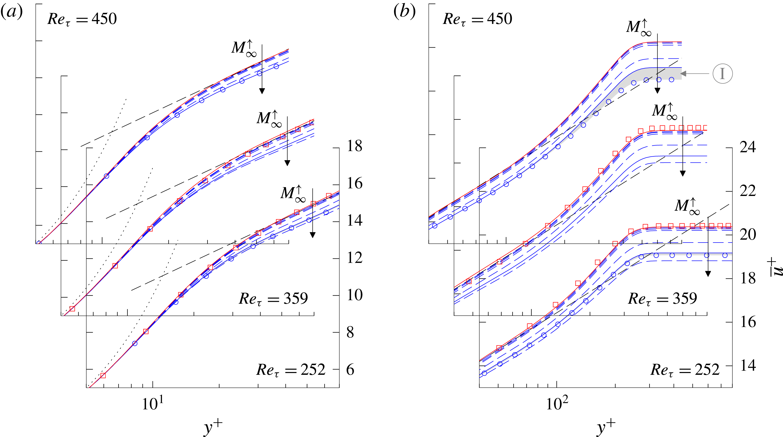
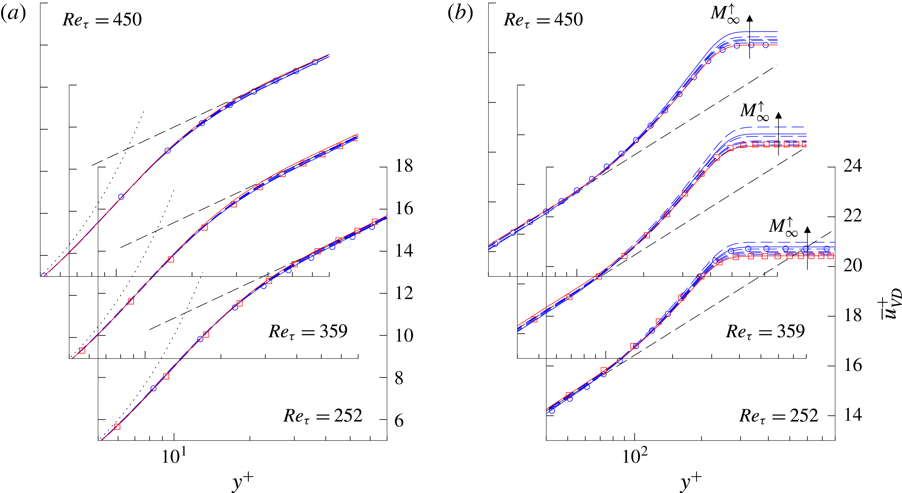
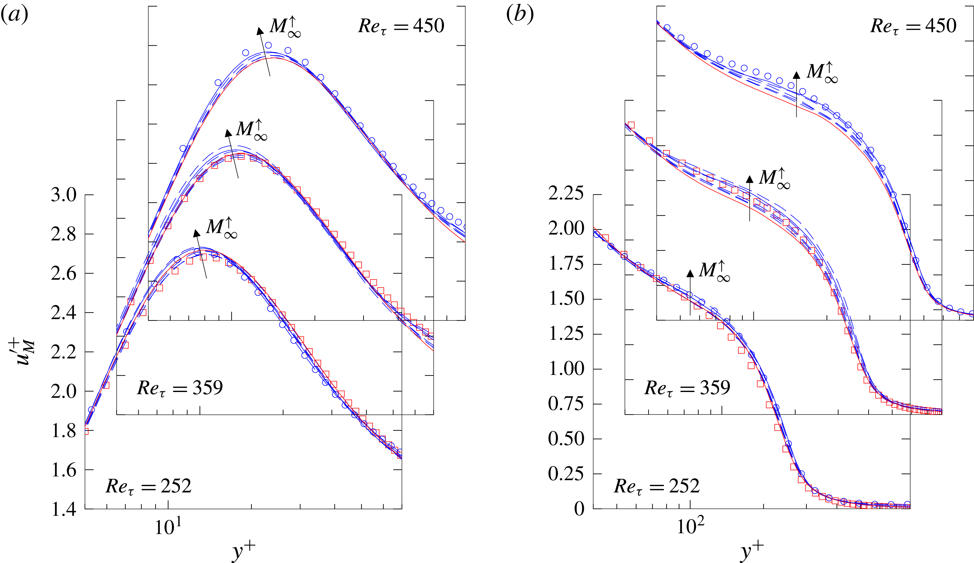
are given in figure 8, calculated by (5.3). The inner layer of the boundary layer – including the viscous sublayer and the inner part of the logarithmic layer – is given on the left-hand side in figures 7(a) and 8(a), respectively, whereas its outer part with the wake region is given on the right-hand side in figures 7(b) and 8(b). The theoretical curves for the viscous sublayer
 $y^{+}=\overline{u}_{(VD)}^{+}$
and the logarithmic layer
 $\overline{u}_{(VD)}^{+}=1/k\,\ln y^{+}+C$
with
 $k=0.41$
and
 $C=5.2$
are given by black-dotted lines and black-dashed lines, respectively. All figures show velocity distributions at the same three Reynolds numbers
 $Re_{\unicode[STIX]{x1D70F}}=252$
, 359 and 450, staggered diagonally in ascending order. The scale for the axes is the same for each Reynolds number and is given for clarity only for the foremost coordinate system. Reference data are depicted with red non-filled squares for the incompressible simulation by Schlatter & Örlü (Reference Schlatter and Örlü2010) at
 $Re_{\unicode[STIX]{x1D70F}}=252$
and 359 and blue non-filled circles for the
 $M_{\infty }=2.0$
simulation by Pirozzoli & Bernardini (Reference Pirozzoli and Bernardini2011) at
 $Re_{\unicode[STIX]{x1D70F}}=252$
and 450. It should be noted that the precise accordance of the desired skin-friction Reynolds numbers
 $Re_{\unicode[STIX]{x1D70F}}=\overline{\unicode[STIX]{x1D70C}}_{w}^{\ast }u_{\unicode[STIX]{x1D70F}}^{\ast }\unicode[STIX]{x1D6FF}_{99}^{\ast }/\overline{\unicode[STIX]{x1D707}}_{w}^{\ast }$
leads to an exact agreement of the non-dimensionalized boundary-layer thicknesses
 $\unicode[STIX]{x1D6FF}_{99}^{+}=\overline{\unicode[STIX]{x1D70C}}_{w}^{\ast }u_{\unicode[STIX]{x1D70F}}^{\ast }\unicode[STIX]{x1D6FF}_{99}^{\ast }/\overline{\unicode[STIX]{x1D707}}_{w}^{\ast }$
. Consequently, the boundary-layer edge
 $\unicode[STIX]{x1D6FF}_{99}^{+}=Re_{\unicode[STIX]{x1D70F}}$
is located at identical
 $y^{+}$
-values for all Mach numbers in every sub-plot.
Comparison of present mean-velocity profiles with incompressible (Schlatter & Örlü Reference Schlatter and Örlü2010 ▫ (red)) and compressible reference data at
 $M_{\infty }=2.0$
(Pirozzoli & Bernardini (Reference Pirozzoli and Bernardini2011) ○ (blue)) at
 $Re_{\unicode[STIX]{x1D70F}}=252$
, 359 and 450. Present results are represented for the
 $M_{\infty }=0.3$
case by solid red lines (——), for the
 $M_{\infty }=2.0$
case by solid blue lines (——) and the remaining cases by dashed blue lines (– –). Arrows denote the direction of increasing Mach number. The dotted lines denote the viscous sublayer with
 $\overline{u}^{+}=y^{+}$
whereas the dashed black lines denote the logarithmic region with
 $\overline{u}^{+}=1/k\,\ln y^{+}+C$
with
 $k=0.41$
and
 $C=5.2$
;
 $y^{+}=y^{\ast }u_{\unicode[STIX]{x1D70F}}^{\ast }/\overline{\unicode[STIX]{x1D708}}_{w}^{\ast }$
.

Same as figure 7 but for van-Driest-transformed profiles
 $\overline{u}_{VD}^{+}$
.

According to the previous section, our simulation results are distinguished between red lines for the quasi-incompressible results at
 $M_{\infty }=0.3$
and blue lines for higher-Mach-number cases. For better clarity, only the results according to the reference data at
 $M_{\infty }=0.3$
and
 $M_{\infty }=2.0$
are represented by solid lines. Since compressible results for
 $M_{\infty }=0.5$
, 0.7, 0.85, 1.5 and 2.5 are not considered in detail but represent important trends, all of them are denoted by dashed lines without being further distinguished. For better clarification, the direction of increasing Mach numbers is denoted by arrows. Additional information about the presented simulation results in terms of
 $Re_{\unicode[STIX]{x1D703}}$
,
 $c_{f}$
and
 $H_{12}$
can be extracted from figures 3–5, where the filled symbols ( ▪ (red),
 $\star$
, ▴, ♦, ◂, ●, ▸ (blue)) denote the positions where the local velocity profiles are extracted. Owing to the skin-friction Reynolds-number shift caused by compressibility (see figure 4 for instance), no results are available for
 $M_{\infty }=2.5$
in the rearmost plot at
 $Re_{\unicode[STIX]{x1D70F}}=450$
in the following.
First, only the compressible mean-flow velocity distributions are analysed in figure 7, without being van-Driest transformed. A comparison between the incompressible reference (▫ (red)) and the
 $M_{\infty }=0.3$
case (red solid line) for
 $Re_{\unicode[STIX]{x1D70F}}=252$
and 359 confirms the excellent agreement, which has already been determined for the spatial evolution of mean-flow data in the previous section. This agreement also holds for higher Reynolds numbers up to
 $Re_{\unicode[STIX]{x1D70F}}\approx 943$
, which are not given in this publication. Thus, the
 $M_{\infty }=0.3$
case can be used as incompressible reference for Reynolds numbers where no incompressible validation data are available in the literature. A comparison of the compressible results shows the expected compressibility shift in the logarithmic layer and wake region towards lower
 $\overline{u}^{+}$
-values, while the viscous sublayer (
 $y^{+}\lesssim 10$
) is completely unaffected. If special focus is put on the comparison of the subsonic cases, compressibility influences of about 2 % can be quantified in the wake region between the
 $M_{\infty }=0.85$
and
 $M_{\infty }=0.3$
cases, whereas the
 $\overline{u}^{+}$
-values are decreased by about 1 % in the logarithmic region. A more detailed look at the subsonic cases can be found in Wenzel et al. (Reference Wenzel, Selent, Kloker and Rist2017). If the
 $M_{\infty }=2.0$
case in particular (blue solid lines) is compared to Pirozzoli & Bernardini’s reference (○ (blue)), a perfect match can be observed in the logarithmic layer for
 $Re_{\unicode[STIX]{x1D70F}}=252$
and 450. Whereas this agreement also holds for the wake region at
 $Re_{\unicode[STIX]{x1D70F}}=252$
, significant differences can be found at
 $Re_{\unicode[STIX]{x1D70F}}=450$
(grey shaded area Ⓘ in figure 7
b). However it is well known from the literature that the wake region is massively influenced by history effects resulting from the inlet boundary condition. Whereas both the viscous sublayer and the logarithmic region adjust rapidly to consistent states due to their close proximity to the wall (Spalart, Strelets & Travin Reference Spalart, Strelets and Travin2006), the outer flow is affected in the order of fifty to hundred boundary-layer thicknesses by the inlet, depending on the inflow quality. For higher Reynolds numbers, this problem becomes even more compelling due to larger boundary-layer thicknesses including an increased number of turbulent structures and slowing down boundary-layer growth (Stiegler Reference Stiegler2017). Since Pirozzoli & Bernardini’s high-Reynolds-number case at
 $Re_{\unicode[STIX]{x1D70F}}=450$
is simulated in a second domain by applying a turbulent inlet-boundary condition once again, we attribute our results a higher reliability. It should be recalled that slightly different trends also have been observed between Pirozzoli & Bernardini’s three simulation domains in the discussion of figure 4 before. Nevertheless, the existence of such relatively large differences in the local mean-flow distribution had not been expected from these investigations.
If the van-Driest-transformed velocity profiles
 $\overline{u}_{VD}^{+}$
are considered (figure 8), the viscous sublayer seems to be only infinitesimally affected by the van-Driest transformation and the determined agreement between the different Mach-number cases remains unchanged. Even though this observation is extensively validated in literature, this is worth mentioning since the van-Driest transformation was derived in a strict sense only for the logarithmic layer. When the logarithmic layers of the van-Driest-transformed velocity profiles are compared to the incompressible reference (○ (blue)) or the
 $M_{\infty }=0.3$
case (red solid line), the generally accepted incompressible logarithmic-law constants of
 $k=0.41$
and
 $C=5.2$
can also be confirmed from this study. Even if the present data could hint that
 $C$
is slightly reduced for the higher Mach-number cases, no conclusive statements seem appropriate due to uncertainties in the numerical data range. A comparison between the wake regions for the different Mach-number cases (figure 8
b) shows a rising trend for increasing Mach numbers at the boundary-layer edge
 $y^{+}=\unicode[STIX]{x1D6FF}_{99}^{+}=Re_{\unicode[STIX]{x1D70F}}$
. This trend is in accordance with Pirozzoli & Bernardini’s data for
 $Re_{\unicode[STIX]{x1D70F}}=252$
, where reference data (○ (blue)) and present data (blue solid line) are in good agreement. Whereas this trend is continued by our data for higher Reynolds numbers also, Pirozzoli & Bernardini’s data show perfect agreement with our incompressible reference at
 $Re_{\unicode[STIX]{x1D70F}}=450$
. The difference between our
 $M_{\infty }=2.0$
data (blue solid line) and the reference (○ (blue)) is approximately equal to the difference which has already been observed and analysed in the discussion of figure 7(b) (grey shaded region Ⓘ).
In conclusion it can be clearly seen that no commonly accepted mean-flow profile exists for the wake region of compressible turbulent boundary layers in the literature, since even the most reliable DNS data may be affected by the numerical set-up especially for higher Reynolds numbers. In order to reconcile this disagreement, the spatial evolution of the wake region is quantitatively analysed in the following with the objective of finding an appropriate Reynolds number for its derivation.
5.3 Mixing length and wake region
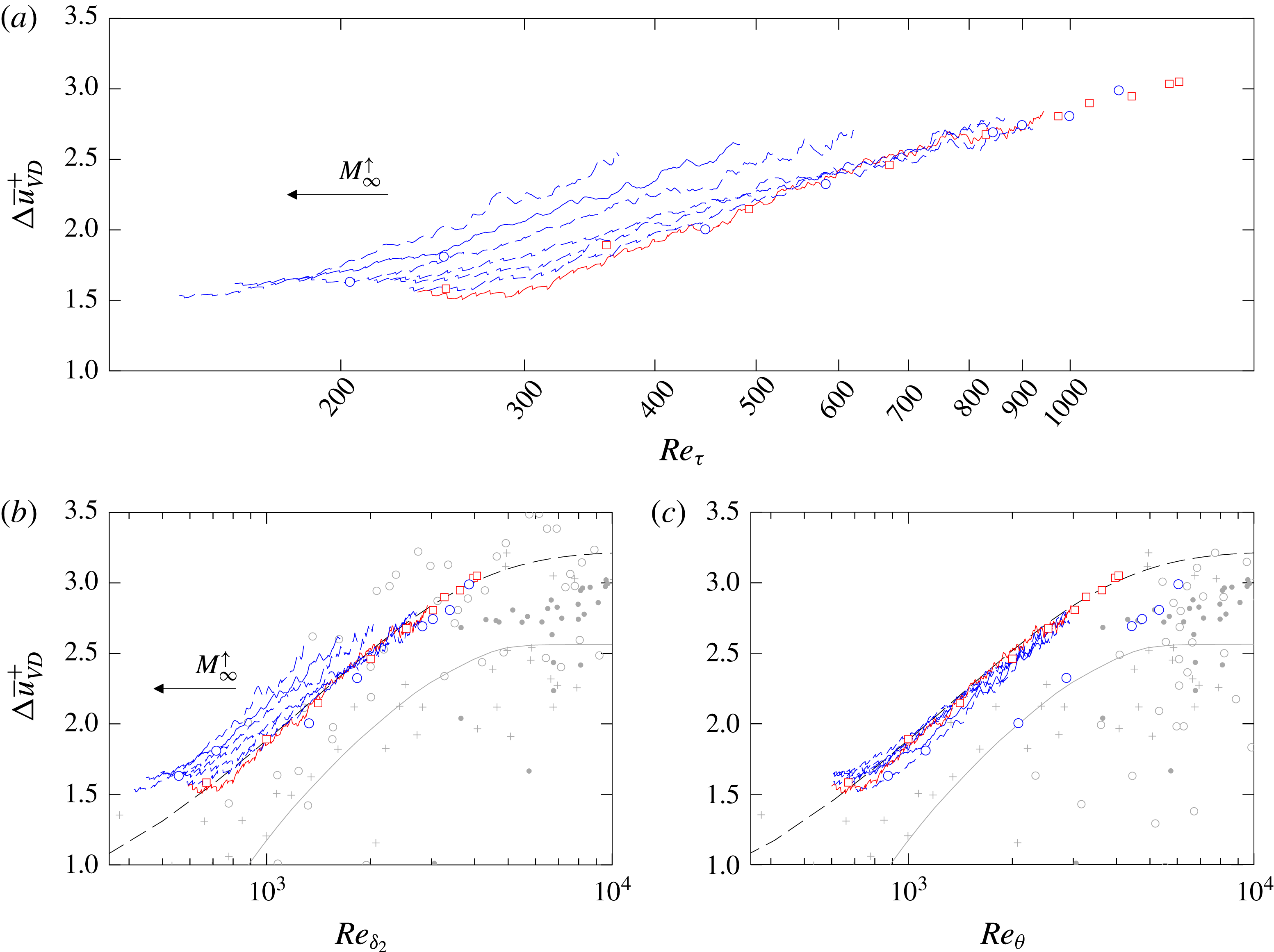
It was found by Coles (Reference Coles1956) that the deviation of the
 $\overline{u}^{+}$
-velocity profile in the wake region from the logarithmic law
 $\unicode[STIX]{x0394}\overline{u}^{+}=\overline{u}^{+}-(1/k\,\ln y^{+}+C)$
shares a similar form in all incompressible cases. By adding a law-of-the-wake to the law-of-the-wall, he proposed a scaling law for the velocity profiles in incompressible TBLs which describes the velocity profile from the inner edge of the logarithmic region all the way to the edge of the boundary layer (Smits & Dussauge Reference Smits and Dussauge2006). By representing the shape of the turbulent wake with the function
 $w(y/\unicode[STIX]{x1D6FF}_{99})$
(Coles’ wake function), this yields
 $$\begin{eqnarray}\overline{u}^{+}=\frac{1}{k}\ln y^{+}+C+\frac{\unicode[STIX]{x1D6F1}}{k}w\left(\frac{y}{\unicode[STIX]{x1D6FF}_{99}}\right).\end{eqnarray}$$
The parameter
 $\unicode[STIX]{x1D6F1}$
is known as the wake-strength parameter and can be easily determined by simply measuring the deviation of the velocity profile from the logarithmic law at the boundary-layer edge
 $\unicode[STIX]{x1D6FF}_{99}$
where Coles’ wake function becomes 2(
 $\unicode[STIX]{x0394}\overline{u}^{+}(y=\unicode[STIX]{x1D6FF}_{99})=2\unicode[STIX]{x1D6F1}/k$
). The wake-strength value
 $\unicode[STIX]{x1D6F1}$
, however, has not yet been finally determined due to its strong Reynolds-number dependence. Whereas it was found from experimental data that
 $\unicode[STIX]{x1D6F1}$
increases from a zero value at very low Reynolds numbers to an asymptotic value of about
 $0.55{-}0.6$
for
 $k=0.41$
and
 $C=5.0$
at higher Reynolds numbers (Coles Reference Coles1964; Erm, Joubert & Smits Reference Erm, Joubert and Smits1987), the prediction of
 $\unicode[STIX]{x1D6F1}$
is strongly influenced by slight variations in
 $k$
and
 $C$
(Smith Reference Smith1994; Fernholz & Finley Reference Fernholz and Finley1996). At present, both the trend to zero value at low Reynolds numbers and the asymptotic behaviour of
 $\unicode[STIX]{x1D6F1}$
for high Reynolds numbers are not clear and Spalart (Reference Spalart1988) concluded that ‘very accurate measurements or simulations over a wide
 $Re_{\unicode[STIX]{x1D703}}$
range, as well as a strong consensus on the value of
 $k$
will be needed before definitive results can be obtained for
 $\unicode[STIX]{x0394}\overline{u}^{+}$
’ (see Smits & Dussauge (Reference Smits and Dussauge2006) for further information).
In the case of adiabatic compressible TBLs with pressure gradient or isothermal walls with zero pressure gradient, a straightforward extension of Coles’ incompressible wall-wake velocity profile (5.4) has been given by several authors (see Smits & Dussauge Reference Smits and Dussauge2006) by simply replacing
 $\overline{u}^{+}$
with
 $\overline{u}_{VD}^{+}$
in (5.4). In comparison to incompressible flows, however, problems arise due to the strong Reynolds-number dependence of
 $\unicode[STIX]{x1D6F1}$
since the Reynolds number, through which the compressible wake can be scaled, is unknown (see also § 2.1). Even if it was found by the comparison of experimental data that some values for
 $\unicode[STIX]{x1D6F1}$
show comparatively good agreement if they are plotted versus the momentum-thickness Reynolds number calculated with the viscosity at the wall
 $Re_{\unicode[STIX]{x1D6FF}_{2}}$
, it might be expected that the strength-of-the-wake component should be a function of outer-edge quantities and should therefore be a function of
 $Re_{\unicode[STIX]{x1D703}}$
rather than
 $Re_{\unicode[STIX]{x1D6FF}_{2}}$
(Smits & Dussauge Reference Smits and Dussauge2006). This expectation might be supported by some DNS data (Gatski & Bonnet Reference Gatski and Bonnet2013), due to large data scattering in the available data range; however, no conclusive statements about the Mach-number influence on the strength-of-the-wake component seem reasonable.
Wake deficit
 $\unicode[STIX]{x0394}u_{VD}^{+}=2\unicode[STIX]{x1D6F1}/k$
plotted versus (a)
 $Re_{\unicode[STIX]{x1D70F}}$
(b)
 $Re_{\unicode[STIX]{x1D6FF}_{2}}$
and (c)
 $Re_{\unicode[STIX]{x1D703}}$
, compared to incompressible DNS by Schlatter & Örlü (Reference Schlatter and Örlü2010) (▫ (red)) and compressible DNS by Pirozzoli & Bernardini (Reference Pirozzoli and Bernardini2011) ○ (blue). Present results are represented for the
 $M_{\infty }=0.3$
case by solid red lines (——), for the
 $M_{\infty }=2.0$
case by solid blue lines (——) and the remaining cases by dashed blue lines (– –). Arrows denote the direction of increasing Mach number. The grey solid line represents Coles’ mean curve (——), Coles Reference Coles1964), and the dashed black line a re-calibrated Cebeci & Smith’s wake-strength function (– –, see (5.5), Cebeci & Smith (Reference Cebeci and Smith1974)). Other references (mainly experimental) are explained in the text.

Plotted versus the Reynolds numbers
 $Re_{\unicode[STIX]{x1D70F}}$
,
 $Re_{\unicode[STIX]{x1D6FF}_{2}}$
and
 $Re_{\unicode[STIX]{x1D703}}$
, figure 9 gives the distance
 $\unicode[STIX]{x0394}\overline{u}_{VD}^{+}=2\unicode[STIX]{x1D6F1}/k$
between the van-Driest-transformed velocity profile
 $\overline{u}_{VD}^{+}$
at the boundary-layer edge
 $\unicode[STIX]{x1D6FF}_{99}^{+}$
and the logarithmic law with
 $k=0.41$
and
 $C=5.2$
for all Mach numbers. In continuation of the previous section, all data are compared to the incompressible and compressible reference data at
 $M_{\infty }=2.0$
(Schlatter & Örlü (Reference Schlatter and Örlü2010) ▫ (red); Pirozzoli & Bernardini (Reference Pirozzoli and Bernardini2011) ○ (blue)). Additionally, experimental reference data are given by grey crosses (
 $+$
) for incompressible data (Fernholz & Finley (Reference Fernholz and Finley1996)) and non-filled grey circles (○) for compressible data (Fernholz & Finley Reference Fernholz and Finley1980), respectively. The grey solid line represents Coles’ mean curve (Coles Reference Coles1964). Both the experimental reference data and Coles’ mean curve are calculated for logarithmic law constants of
 $k=0.41$
and
 $C=5.0$
in contrast to our constants of
 $k=0.41$
and
 $C=5.2$
. To account for the variations in
 $C$
, these data are shifted by the difference
 $\unicode[STIX]{x0394}C=0.2$
downwards by the present authors. Since it could not be clarified whether the skin-friction velocity
 $u_{\unicode[STIX]{x1D70F}}$
has been derived consistently for all experimental data from the best fit on the theoretical law with
 $C=5.0$
, no further compensatory approaches have been attempted. Grey filled circles represent results which are calculated from the experimental incompressible data provided by Österlund (Reference Österlund1999).
If the nearly incompressible results at
 $M_{\infty }=0.3$
(red solid line) are compared to the incompressible reference in figure 9(a–c) first (▫ (red)), an excellent agreement can be observed especially for higher Reynolds numbers, where the influence of the turbulent inlet boundary condition decreases. This agreement is noteworthy especially against the background of the sensitivity of the wake parameters to the numerical set-up which has already been seen in the discussion of figures 7 and 8.
If the compressible results (blue lines) are assessed in the following for figure 9(a) first by plotting versus
 $Re_{\unicode[STIX]{x1D70F}}$
, the weakness of the van-Driest transformation in the wake region can be quantified by the shift of the wake strength parameter towards higher values. This shift corresponds to the deviation between the van-Driest-transformed mean-velocity profiles
 $\overline{u}_{VD}^{+}$
and the logarithmic law (black dashed line), measured at the boundary-layer edge
 $y^{+}=\unicode[STIX]{x1D6FF}_{99}^{+}=Re_{\unicode[STIX]{x1D70F}}$
in figure 8(b). Consistency between the compressible reference (○ (blue)) and our
 $M_{\infty }=2.0$
case (blue solid line) can only be observed for Pirozzoli & Bernardini’s first simulation domain up to
 $Re_{\unicode[STIX]{x1D70F}}=273$
. For higher Reynolds numbers, Pirozzoli & Bernardini’s results follow our nearly incompressible reference case (red solid line). This behaviour can be traced back to distorting influences caused by the turbulent inflow boundary condition and has been already discussed in the previous section.
According to the literature, the wake region could be scaled either with
 $Re_{\unicode[STIX]{x1D6FF}_{2}}$
or
 $Re_{\unicode[STIX]{x1D703}}$
, amongst many other possibilities. Plotted against both
 $Re_{\unicode[STIX]{x1D6FF}_{2}}$
and
 $Re_{\unicode[STIX]{x1D703}}$
, the wake deficit
 $\unicode[STIX]{x0394}\overline{u}_{VD}^{+}$
is given in figures 9(b) and 9(c), respectively. Whereas it seems that the compressible experimental reference data (○ (grey)) are fitted much better by Coles’ mean curve (grey solid line) by plotting at the same
 $Re_{\unicode[STIX]{x1D6FF}_{2}}$
in contrast to
 $Re_{\unicode[STIX]{x1D703}}$
, our data are almost perfectly scaled by
 $Re_{\unicode[STIX]{x1D703}}$
. Even if the comparison at the same
 $Re_{\unicode[STIX]{x1D6FF}_{2}}$
also represents an improvement compared to plotting at the same
 $Re_{\unicode[STIX]{x1D70F}}$
, a clear Mach-number trend can still be observed in this case. Nevertheless, it cannot be excluded that other (maybe very complex) Reynolds-number definitions exist, which can scale the compressible wake even better than
 $Re_{\unicode[STIX]{x1D703}}$
. However, the nearly perfect scaling of our data at the same
 $Re_{\unicode[STIX]{x1D703}}$
strongly affirms the intuitive expectation that any kind of Reynolds number which scales the strength-of-the-wake component has to be a function of outer-edge quantities rather than wall quantities as described before. At this point, once again, we want to emphasize the difficulty in the assessment of CTBL-DNS data by comparing Pirozzoli & Bernardini’s compressible data (○ (blue)) to our results. All three of their simulations have been proven to be the most reliable in the literature, but no conclusive statements can be obtained from their data for the scaling of the compressible wake. The same holds true for the experimental data range, which significantly suffers from uncertainties in the measurement techniques at such low Reynolds numbers (see Smits & Dussauge Reference Smits and Dussauge2006). Most of the experimental data show wake-deficit values being significantly lower than the present results.
To account for the strong variations of the presented data range, the non-zero value of our data at low Reynolds numbers and the trend to higher
 $\unicode[STIX]{x1D6F1}$
values for higher Reynolds numbers, a re-calibration of Cebeci & Smith’s wake-strength function is provided (Cebeci & Smith Reference Cebeci and Smith1974). The re-calibrated formulation states
 $$\begin{eqnarray}\unicode[STIX]{x1D6F1}=0.66(1-\exp (-0.4Z^{0.5}-0.48Z)),\quad Z=\frac{Re_{\unicode[STIX]{x1D703}}}{1000}.\end{eqnarray}$$
This formulation is represented in figure 9(b,c) by a dashed black line. It should be mentioned that the asymptotic trend of the re-calibrated formulation for higher Reynolds numbers is just a rough guess. Even if one tried by the use of Österlund’s experimental data-set (Österlund Reference Österlund1999) (● (grey)) to get an impression of
 $\unicode[STIX]{x1D6F1}$
’s high-Reynolds-number behaviour, no conclusive statements seem to be appropriate in this regime due to data scattering. For final clarification, DNS have to be performed with only one set-up beginning at very low Reynolds numbers and ending at spectacularly high Reynolds numbers.
5.4 Statistics of local averaged velocity fluctuations
In this section, the distribution of the Reynolds fluctuations is analysed with particular regard to Morkovin’s hypothesis, yielding the Morkovin scaling (see § 5.2). For clarity, only the streamwise velocity component
 $u^{\prime +}$
is presented in the main part of this work whereas the wall-normal and spanwise components
 $v^{\prime +}$
and
 $w^{\prime +}$
are given in appendix B. Both non-dimensionalized in wall units, the profiles of the streamwise Reynolds fluctuations
 $u^{\prime +}=\sqrt{\overline{u^{\prime }u^{\prime }}}/u_{\unicode[STIX]{x1D70F}}$
are given in figure 10 whereas the density-scaled Reynolds fluctuations
 $u_{M}^{\prime +}=\sqrt{\overline{\unicode[STIX]{x1D70C}}/\unicode[STIX]{x1D70C}_{w}}\sqrt{\overline{u^{\prime }u^{\prime }}}/u_{\unicode[STIX]{x1D70F}}$
(Morkovin transformed) are given in figure 11. According to the mean-flow profiles given in § 5.2, the inner layer is shown on the left-hand side in figures 10(a) and 11(a), whereas the outer layer is shown on the right-hand side in figures 10(b) and 11(b), respectively. The exact spatial position where the distributions are extracted from the simulation domain in terms of
 $Re_{\unicode[STIX]{x1D70F}}$
corresponds to the filled symbols given in figure 6 (▪ (red),
 $\star$
, ▴, ♦, ◂, ●, ▸ (blue)). The representation of both the reference data and our results is in accordance with the mean-flow study in § 5.2 above. In order to provide a better comparability, also the
 $y^{+}$
-axis scaling is the same as for the mean-flow profiles in figures 7 and 8.
Comparison of streamwise Reynolds fluctuations
 $u^{\prime +}=\sqrt{\overline{u^{\prime }u^{\prime }}}/u_{\unicode[STIX]{x1D70F}}$
with incompressible reference (Schlatter & Örlü Reference Schlatter and Örlü2010 ▫ (red)) and compressible reference for
 $M_{\infty }=2.0$
(Pirozzoli & Bernardini Reference Pirozzoli and Bernardini2011 ○ (blue)) for
 $Re_{\unicode[STIX]{x1D70F}}=252$
, 359 and 450. Present results are represented for the
 $M_{\infty }=0.3$
case by solid red lines (——), for the
 $M_{\infty }=2.0$
case by solid blue lines (——) and the remaining cases by dashed blue lines (– –). The direction of increasing Mach number is denoted by arrows.

Same as figure 10 but for density-scaled streamwise Reynolds fluctuations,
 $u_{M}^{\prime +}=\sqrt{\overline{\unicode[STIX]{x1D70C}}/\unicode[STIX]{x1D70C}_{w}}\sqrt{\overline{u^{\prime }u^{\prime }}}/u_{\unicode[STIX]{x1D70F}}$
.

If the streamwise Reynolds fluctuations are analysed in their original formulation in figure 10 first, a good agreement can be found between the nearly incompressible case at
 $M_{\infty }=0.3$
(red solid line) and the incompressible reference data (Schlatter & Örlü Reference Schlatter and Örlü2010, ▫ (red)) for
 $Re_{\unicode[STIX]{x1D70F}}=359$
in the peak region up to
 $y^{+}\approx 30$
. In the outer layer, our data lie by about 3 % below the incompressible reference. As already has been seen in the discussion of figure 6, the peak value of
 $u^{\prime +}$
is slightly too high at
 $Re_{\unicode[STIX]{x1D70F}}=252$
(red solid line) since it is still influenced by the inflow boundary condition. If this shift is also assumed to hold in the outer region of the boundary layer for
 $Re_{\unicode[STIX]{x1D70F}}=252$
, the same discrepancies which have been observed at
 $Re_{\unicode[STIX]{x1D70F}}=359$
for the incompressible reference are expected to exist in an undistorted representation. A comparison between the
 $M_{\infty }=2.0$
case and Pirozzoli & Bernardini’s compressible reference data (○ (blue)) shows excellent agreement both for
 $Re_{\unicode[STIX]{x1D70F}}=252$
and 450. Small differences, especially in the peak value, have already been discussed with figure 6 but do not question the agreement between the given data. This agreement is remarkable especially in the outer region at
 $Re_{\unicode[STIX]{x1D70F}}=450$
, where significant differences in the mean-value distribution of the streamwise velocity field have been found in the discussion of figure 7 above. It must be concluded therefore that the exact mean value around which the velocity field fluctuates does not play a major role in the fluctuation’s distribution. According to figure 6, a comparison between the different Mach number cases shows a shift of the
 $u^{\prime +}$
peak towards lower
 $u^{\prime +}$
values at lower wall-normal positions
 $y^{+}$
. In the outer layer, the
 $u^{\prime +}$
-distribution seems to be just shifted from the incompressible reference.
Having a closer look at the density-transformed velocity fluctuations in figure 11(a), the peak of the velocity shows a clear trend towards higher
 $u^{\prime +}$
-values which are located closer to the wall in terms of
 $y^{+}$
for increasing Mach numbers. This trend seems to be confirmed by the agreement between our data and both the compressible and incompressible reference data, which show a comparable trend in the peak region. If the outer region of the Morkovin-transformed profiles is compared in figure 11(b), no perfect match between the compressible data can be obtained either, since the absolute level of the outer plateau is lifted up for higher Mach numbers. Additionally this trend seems to be confirmed by the reference data, which are in very good agreement with our data at
 $M_{\infty }=2.0$
. Moreover, if the fluctuating profiles for
 $v^{\prime +}$
and
 $w^{\prime +}$
are analysed (appendix B), noticeable Mach number influences can be found over the whole boundary-layer thickness, also increasing the incompressible velocity distributions by a comparable magnitude.
Even if none of the described differences are strong enough to qualitatively question Morkovin’s hypothesis, truly incompressible reference data cannot be used to validate DNS data of CTBLs even at moderate Mach numbers, if compressible data are sought to be confirmed with high accuracy. Due to the enormous increase in computational power, however, we think that it is the primary task of present day DNS to provide this level of reliability if very accurate investigations are to be performed for compressible turbulent flows.
5.5 Statistics of local averaged thermodynamic fluctuations
Whereas the previous analysis has focused on the evaluation of the velocity field, the fluctuation of thermodynamical variables will be analysed in this section. Therefore, the distribution of the temperature fluctuations
 $T^{\prime +}=\sqrt{\overline{T^{\prime 2}}}/(\unicode[STIX]{x1D6FE}M_{\infty }^{2}u_{\unicode[STIX]{x1D70F}}^{2})$
as well as the distribution of the density fluctuations
 $\unicode[STIX]{x1D70C}^{\prime +}=\sqrt{\overline{\unicode[STIX]{x1D70C}^{\prime 2}}}/\overline{\unicode[STIX]{x1D70C}}_{w}$
are compared in figures 12(a) and 12(b) respectively, in inner scaling. Since highly reliable compressible reference data are only available for the lowest Reynolds number at
 $Re_{\unicode[STIX]{x1D70F}}=252$
for
 $M_{\infty }=2.0$
, only these data are compared in the following. In accordance with the previous sections, incompressible results are denoted by red solid lines and compressible results by blue lines. The compressible reference at
 $M_{\infty }=2.0$
from Pirozzoli & Bernardini (Reference Pirozzoli and Bernardini2011) is denoted by blue circular non-filled symbols and should be compared to our
 $M_{\infty }=2.0$
case, which is distinguished from other compressible results by a solid blue line.
The comparison of the temperature fluctuations
 $T^{\prime +}$
in figure 12(a) shows a clear trend to lower
 $T^{\prime +}$
values for increasing Mach numbers in inner scaling over the whole logarithmic and wake region. In contrast to the compressible reference at
 $M_{\infty }=2.0$
, which is simulated with a pseudo-adiabatic wall-temperature boundary condition, the temperature fluctuations do not drop to zero at the wall when truly adiabatic boundary conditions are applied. Against this background, the excellent agreement between the provided reference (○ (blue)) and our data for
 $y^{+}\gtrsim 8$
at
 $M_{\infty }=2.0$
(blue solid line) is underlined. Since the influence of the temperature boundary condition is found to be restricted to the viscous sublayer and no differences have been found in the provided data before, CTBLs do not seem to be significantly influenced by the choice of the adiabatic temperature boundary condition, if the prescribed mean-temperature value is calculated correctly.
In contrast to the temperature fluctuations, the inner-scaled density fluctuations are strongly enhanced for higher Mach numbers, see figure 12(b). The non-zero constant value of the density fluctuations in the direct vicinity of the wall for
 $y^{+}\lesssim 3$
is not a result of the adiabatic boundary condition, since the present (solid blue line) and Pirozzoli & Bernardini’s data (○ (blue)) are in perfect agreement directly at the wall. A comparison of the curve progressions between the different Mach numbers show a more evident dent at
 $y^{+}\approx 2\times 10^{2}$
for increasing Mach numbers. Whereas this peak is less dominant for
 $M_{\infty }\lesssim 2.0$
compared to the inner peak at
 $y^{+}\approx 2\times 10^{1}$
, both are at approximately the same level for
 $M_{\infty }\approx 2.0$
. For higher Mach numbers, the outer peak noticeably exceeds the inner peak. The altered shape of the density distributions therefore does not allow a reconstruction of the density fluctuations for higher Mach numbers by a simple stretching of the
 $M_{\infty }=0.3$
case with an adjusted
 $\overline{\unicode[STIX]{x1D70C}}_{w}$
-value.
Comparison of temperature fluctuations
 $T^{\prime +}$
and density fluctuations
 $\unicode[STIX]{x1D70C}^{\prime +}$
in inner scaling for
 $Re_{\unicode[STIX]{x1D70F}}=252$
. Compressible reference data are taken from Pirozzoli & Bernardini (Reference Pirozzoli and Bernardini2011) (○ (blue)) at
 $M_{\infty }=2.0$
. Present results are represented for the
 $M_{\infty }=0.3$
case by solid red lines (——), for the
 $M_{\infty }=2.0$
case by solid blue lines (——) and the remaining cases by dashed blue lines (– –). Arrows denote the direction of increasing Mach number.

5.6 Statistics of turbulent Mach number and total temperature fluctuations
Next to the van-Driest transformation and Morkovin’s hypothesis, the strong Reynolds analogy is the most important relation in compressible turbulence research, since it couples temperature variations to the fluctuating velocity flow field (Young Reference Young1953; Morkovin Reference Morkovin and Favre1961). Due to its enormous importance for the understanding of basic mechanisms in the compressible regime, the strong Reynolds analogy is one of the most extensively studied topics in CTBL research. The probably most relevant and complete work in terms of DNS is given in Guarini et al. (Reference Guarini, Moser, Shariff and Wray2000) with a TDNS approach for
 $M_{\infty }=2.5$
, see table 1, which is still often used as reference today. Due to its relevance for turbulence research, it is the main objective of this section to assess Guarini et al.’s data by comparison with our SDNS data. To this end, all plots shown by Guarini et al. (Reference Guarini, Moser, Shariff and Wray2000) have been reproduced. A detailed analysis of these plots brought up only slight quantitative differences which do not question any conclusions about compressible turbulence given in Guarini et al. (Reference Guarini, Moser, Shariff and Wray2000). Consequently, only the most important results are described in the following in terms of providing a more continuous path from the incompressible to the compressible regime.
According to Morkovin (Reference Morkovin and Favre1961), Morkovin’s density scaling and the van-Driest transformation are expected to hold if turbulence is only weakly affected by compressibility, which seems to be appropriate for turbulent Mach-number values of
 $M^{\prime }=\sqrt{\overline{M^{\prime }M^{\prime }}}\lesssim 0.2$
(0.3 according to Spina et al. (Reference Spina, Smits and Robinson1994)). Duan et al. (Reference Duan, Beekman and Martin2011), in contrast, have shown for TDNS that this restriction seems to be too strict if compressible scaling laws are only qualitatively analysed. Since our results have shown compressibility effects in the scaling laws even for very low Mach numbers, a resurveyed analysis of the turbulent Mach-number fluctuations seems to be desirable.
Comparison of (a) turbulent Mach number fluctuations
 $M_{t}$
(——) and
 $\overline{M^{\prime 2}}^{1/2}$
(– – –) and (b) (total-)temperature fluctuations
 $\overline{T_{0}^{\prime 2}}^{1/2}/\overline{T}_{0}$
(——),
 $\overline{T_{0}^{\prime 2}}^{1/2}/\overline{T}$
(– – –) and
 $\overline{T^{\prime 2}}^{1/2}/\overline{T}$
(– ⋅ – ⋅ –) in outer scaling for
 $Re_{\unicode[STIX]{x1D70F}}=252$
. Incompressible results are colored in red, compressible in blue. Grey coloured reference is taken from Guarini et al. (Reference Guarini, Moser, Shariff and Wray2000). Arrows denote the direction of increasing Mach number.

A second look at the influence of compressibility on TBLs – and in particular the validity of the strong Reynolds analogy – can be taken by visualizing the distribution of the total-temperature fluctuations
 $T_{0}^{\prime }$
. Even if these are implied to be zero by direct derivation from the strong Reynolds analogy, it is well known that they are comparable in magnitude to the static-temperature fluctuations and therefore definitively non-negligible (Morkovin Reference Morkovin and Favre1961; Guarini et al.
Reference Guarini, Moser, Shariff and Wray2000). Since early relations are mainly derived by assuming negligible fluctuations of the total temperature, there is still progress made in the derivation of more complete (also implying more complex) relations coupling the turbulent temperature with the turbulent velocity field.
Distributions of the fluctuating Mach number
 $M^{\prime }$
as well as the turbulent Mach number
 $M_{t}=\sqrt{\overline{u_{i}^{\prime }u_{i}^{\prime }}}/\overline{a}$
are given in figure 13(a). Whereas
 $M_{t}$
is just a simple scaling of the Reynolds fluctuations with the averaged speed of sound,
 $M^{\prime }$
also takes fluctuations in the speed of sound into account. The distribution of the temperature fluctuations
 $\sqrt{\overline{T_{0}^{\prime }T_{0}^{\prime }}}/\overline{T}_{0}$
,
 $\sqrt{\overline{T_{0}^{\prime }T_{0}^{\prime }}}/\overline{T}$
and
 $\sqrt{\overline{T^{\prime }T^{\prime }}}/\overline{T}$
are presented in figure 13(b), non-dimensionalized by the local total- or static-temperature distribution, respectively. In accordance with Guarini et al. (Reference Guarini, Moser, Shariff and Wray2000), both figure 13(a and 13
b) are plotted versus
 $y/\unicode[STIX]{x1D6FF}_{99}$
. For clarity, only data at
 $Re_{\unicode[STIX]{x1D70F}}=252$
are given in diagonally staggered ascending order for increasing Mach numbers of
 $M_{\infty }=0.3$
–
 $2.5$
. Guarini et al.’s reference data are shown in the rearmost plot for
 $M_{\infty }=2.5$
by grey lines for comparison; the Reynolds number used does not exactly correspond to ours, but lies in an acceptable proximity and allows meaningful comparison (compare most left ▸ (blue) symbol with

 $y/\unicode[STIX]{x1D6FF}_{99}$
-axis due to a different definition of the boundary-layer edge
 $\unicode[STIX]{x1D6FF}_{99}$
, their
 $y/\unicode[STIX]{x1D6FF}_{99}$
-axis is scaled by a factor of 1.22 for better comparability on the corresponding axes. For consistency with the previous investigations, the nearly incompressible case at
 $M_{\infty }=0.3$
is coloured red, whereas higher-Mach-number cases are coloured blue.
If our data on the turbulent Mach-number fluctuations are compared to Guarini et al.’s data in figure 13(a) for
 $M_{\infty }=2.5$
in the rearmost plot, a good agreement can be observed for the peak value of about 0.3, whereas the shoulder shows differences of about 15 % for both
 $M_{t}$
and
 $M^{\prime }$
.
If the temperature distributions are compared in the rearmost plot in figure 13(b), Guarini et al.’s reference data are found to be larger by about 15 %, as already has been seen for the Mach-number fluctuations. Nevertheless, even though a second peak arises in Guarini et al.’s reference data at
 $y/\unicode[STIX]{x1D6FF}_{99}\approx 0.5$
in the static-temperature distribution, both data-sets show a good agreement if only qualitative trends are assessed. According to the current state of knowledge, the total-temperature fluctuations have about the same magnitude as the temperature fluctuations through the whole Mach-number range even for the nearly incompressible case at
 $M_{\infty }=0.3$
; for
 $M_{\infty }=2.5$
the total-temperature fluctuations reach a peak value of about 9 % of the mean static temperature, but are about 2 percentage points lower than with TDNS.
6 Conclusions
Spatial DNS results for CTBLs have been presented in the Mach-number range
 $0.3\leqslant M_{\infty }\leqslant 2.5$
. It is the main goal of this study to provide reliable reference data both for the subsonic and supersonic regimes to prescribe a more continuous path between incompressible and compressible results. We understand that, if the commonly accepted, non-reflecting boundary conditions for far field and outflow are employed in the DNS, there is a unique solution in the statistical sense for the flat-plate set-up, under an identical set of physical parameters. The systematic nature of this study allows a highly reliable quantitative evaluation of traditional compressible scaling laws and the settlement on a commonly accepted compressible mean-flow velocity profile in the considered Mach and Reynolds number range, which is not consistently reported in the literature. Since all investigations are based on an extensively validated, unified data-set with consistency in the numerical set-up and postprocessing for all investigated Mach numbers, these conclusions are quantitatively resilient. In order to assess the quality of our data, these have been compared to an almost complete compilation of the existing literature data-base which shows significant data scattering even in the mean-flow distributions. This comparison also allows a secure assessment of the data-base quality and opens the opportunity to find out which results are therefore highly likely to be reliable.
It was found that the quasi-incompressible case at
 $M_{\infty }=0.3$
as well as the
 $M_{\infty }=2.0$
case are in excellent agreement with the incompressible and compressible benchmark DNS provided by Schlatter et al. (Reference Schlatter, Li, Brethouwer, Johansson and Henningson2010) and Pirozzoli & Bernardini (Reference Pirozzoli and Bernardini2011), for the streamwise evolution of important flow parameters, which consolidates the appraisal of all three simulation setups as being highly reliable. The van-Driest-II transformation was confirmed to provide an excellent, slightly underestimating prediction of the skin-friction coefficient for compressible TBLs as already has been pointed out by Pirozzoli & Bernardini (Reference Pirozzoli and Bernardini2011) by comparison with incompressible reference data, both computed with different numerical set-ups. Temporal DNS and mainly early spatial DNS of CTBLs, however, show consistently large deviations from our data and seem not to be suitable for a quantitative evaluation of compressible scaling laws. The
 $c_{f}$
-distributions obtained by temporal DNS in particular were found to be consistently too large. The particular choice of a truly adiabatic or pseudo-adiabatic temperature boundary condition, however, was found to only affect the temperature fluctuations in the viscous sublayer without changing the mean-flow or fluctuation distributions; in particular, the density fluctuations are not affected.
If special attention is paid to the subsonic Mach-number cases, some palpable compressibility effects exist; this is worth mentioning since subsonic and incompressible Mach numbers are often not distinguished in literature. However, the
 $c_{f}$
- and
 $Re_{\unicode[STIX]{x1D70F}}$
-distributions of all presented subsonic simulations lie in between the scattering of the incompressible DNS data which are available in the literature. Thus, a quantification of Mach-number effects in the subsonic range requires a consistent set-up excluding the concealment of compressibility effects by any non-physical influence like grid effects or different inflow boundary conditions.
The total-temperature fluctuations, assumed to be zero in the strong Reynolds analogy, are found to be consistently non-negligible as elucidated by Guarini et al. (Reference Guarini, Moser, Shariff and Wray2000) at
 $M_{\infty }=2.5$
, rising strongly with increasing Mach number. Our spatial DNS data show a wall-normal distribution being about 13 % less in magnitude than Guarini et al.’s temporal DNS data, but the qualitative behaviour is in full accordance.
For the local mean-flow velocity profiles, the van-Driest transformation is found to not scale the compressible wake region to the incompressible form. In contrast to the general understanding, the wake-strength value
 $2\unicode[STIX]{x1D6F1}/k$
is found to scale in excellent fashion if using the momentum-thickness Reynolds number based on the edge viscosity and not on the wall viscosity, which is in much better accordance with the intuitive feeling that the wake is more influenced by far-field values than by wall values. However, it was shown by the comparison with Pirozzoli & Bernardini’s reference data that the wake region is extremely sensitive to the Reynolds number, where the inlet boundary condition is applied. Whereas Pirozzoli & Bernardini’s results are in perfect agreement with our present results for low Reynolds numbers, a separate simulation starting at higher Reynolds numbers cannot hold this agreement. This fact should also be considered for the assessment of temporal DNS at high Mach numbers, where the boundary-layer thickness is increased and thus the falsifying effect of the periodic domain, compared to incompressible flows at comparable
 $Re_{\unicode[STIX]{x1D70F}}$
.
Like the van-Driest transformation, the validity of Morkovin’s hypothesis for compressibility scaling of the time-averaged velocity fluctuations is influenced by the Mach number. Whereas the peak region of the
 $u^{\prime +}$
-distribution is slightly shifted to higher
 $u^{\prime +}$
-values at lower
 $y^{+}$
-values, the distribution in the wake region is lifted up by about 8 % in the investigated Mach number range due to compressibility. The same holds for the wall-normal and spanwise components
 $v^{\prime +}$
and
 $w^{\prime +}$
, respectively, which both are shifted in a comparable range almost over the entire boundary layer. Even if these effects are not strong enough to qualitatively question Morkovin’s hypothesis, classical scaling is not sufficient to scale compressible data to incompressible laws from a strict DNS point of view. However, since DNS – even in the case of CTBLs as has been shown by comparison with the literature data-base – is able to provide data with uncertainties of less than 1 % if the inlet boundary condition is applied at very low Reynolds numbers, these differences are large enough to claim that classical scaling cannot be used for state-of-the-art DNS-data validation if compressible data are sought to be confirmed with high accuracy. This holds even for the higher subsonic range which is commonly treated to be equivalent to incompressible flow. Due to the enormous increase in computational power, however, we think that it is the primary task of present day DNS to provide this level of accuracy, especially since flow-control investigations must be quantitatively evaluated with great care.
Acknowledgements
The financial support by the Deutsche Forschungsgemeinschaft, DFG, under reference no. RI680/31-1, and the provision of computational resources on the national supercomputer Cray XC40 at the Federal High Performance Computing Center Stuttgart (HLRS) under grant GCS Lamt (LAMTUR) are gratefully acknowledged, as well as fruitful discussions within the DFG Collaborative Research Center SFB/TRR 40(A4).
Appendix A
In this section additional information is given about the auxiliary recycling simulations which are used for the computation of the time-averaged mean-velocity profiles and the Reynolds-fluctuation fields. Both are necessary – generally unknown – input parameters for the SEM inlet boundary condition used for the main simulations, see § 3.3. For the auxiliary simulations, the numerical method as well as the basic thermodynamic flow properties are identical with the main simulations as already described in §§ 3.2 and 3.4.
A sketch of the recycling simulation domain is presented in figure 14. It consists of a fully resolved main region with a dimension of
 $5\unicode[STIX]{x03C0}\unicode[STIX]{x1D6FF}_{99,0}\times 3\unicode[STIX]{x1D6FF}_{99,0}\times \unicode[STIX]{x03C0}\unicode[STIX]{x1D6FF}_{99,0}$
in streamwise, wall-normal and spanwise direction, respectively, including the recycle region with a length of
 $3\unicode[STIX]{x03C0}\unicode[STIX]{x1D6FF}_{99,0}$
and a buffer region with a length of
 $2\unicode[STIX]{x03C0}\unicode[STIX]{x1D6FF}_{99,0}$
. For the
 $M_{\infty }=0.3$
case, the main region covers the Reynolds number range
 $300\leqslant Re_{\unicode[STIX]{x1D703}}\leqslant 450$
. In the outflow region, the numerical grid is exponentially stretched in the streamwise direction and tenth-order implicit filtering is applied to avoid reflections from the outflow boundary (Colonius et al.
Reference Colonius, Lele and Moin1993; Visbal & Gaitonde Reference Visbal and Gaitonde2002). The grid size is
 $230\times 97\times 128$
for the main region and
 $330\times 97\times 128$
for the overall domain. Calculated in wall units, a grid spacing of
 $\unicode[STIX]{x0394}x^{+}=10.5$
,
 $\unicode[STIX]{x0394}y_{1}^{+}=0.9$
and
 $\unicode[STIX]{x0394}z^{+}=3.6$
results at
 $Re_{\unicode[STIX]{x1D703}}=300$
(corresponding to the inlet) for
 $M_{\infty }=0.3$
. Caused by the level of freedom which is introduced to the simulations through the recycling approach in order to allow the self-generation of the flow, a restrictive potential-flow boundary condition is applied at the top of the domain, where
 $\unicode[STIX]{x1D70C}$
,
 $T$
,
 $p$
, and
 $u$
are kept constant. The wall-normal and spanwise velocity components
 $v$
and
 $w$
are calculated by their condition
 $\text{d}/\text{d}y=0$
. Except for the inlet, the remaining boundary conditions are the same as for the main simulations, see § 3.3.
Simulation domain for auxiliary recycling simulation. The yellow coloured region represents a sponge zone, the blue coloured region represents a grid-stretched and spatially filtered region. The red bordered zone represents the main region of the simulation, including the recycle region and the buffer region.

A.1 Recycling approach
At the inlet of the simulation domain, a recycling boundary condition is applied which has been described in its incompressible formulation by Lund et al. (Reference Lund, Wu and Squires1998) and in its extended compressible formulation by Urbin & Knight (Reference Urbin and Knight2001), Stolz & Adams (Reference Stolz and Adams2003), Ferrante & Elghobashi (Reference Ferrante and Elghobashi2004), Sagaut et al. (Reference Sagaut, Garnier, Tromeur, Larcheveque and Labourasse2004) and Xu & Martin (Reference Xu and Martin2004). The basic implementation is closely oriented on the work provided by Lund et al. (Reference Lund, Wu and Squires1998) and Stolz & Adams (Reference Stolz and Adams2003). However it should be mentioned that it is not an easy task to get clean recycling simulations, which are generating their mean-flow profiles on their own. As the result of the artificial periodicity being introduced by the repeated feed of the same flow structures, recycling simulations are usually unstable and show drift phenomena in the calculated mean values (Sagaut et al.
Reference Sagaut, Garnier, Tromeur, Larcheveque and Labourasse2004). Once the flow has been adapted to its final state, natural oscillations occur with wavelengths being multiples of the length of the recycling domain, mainly in the wall-normal velocity component. These are enhanced by the nonlinear character of the Navier–Stokes equations which itself yields a destruction of the flow. To avoid this drift, usually only the velocity fluctuations are rescaled whereas the mean velocity field is fixed to a prescribed distribution, which is, strictly speaking, unknown. A good overview about this problem is given by Sagaut et al. (Reference Sagaut, Garnier, Tromeur, Larcheveque and Labourasse2004). Since we are interested in the mean-velocity profile which is only generated by a real recycling simulation on its own, some effort is necessary to stabilize the simulation as will be described in the following. In order to increase the periodic wavelength of the recycling domain, the recycled flow is re-introduced at the inlet with a spanwise shift of
 $\unicode[STIX]{x03C0}\unicode[STIX]{x1D6FF}_{99,0}/2$
.
Recycling procedure shown, as an example, for the
 $M_{\infty }=0.3$
case. (a) The skin friction velocity ratio
 $u_{\unicode[STIX]{x1D70F},0}/u_{\unicode[STIX]{x1D70F},target}$
of the rescaled velocity profile measured at the inlet of the domain as a function of time;
 $\unicode[STIX]{x0394}t_{1}$
,
 $\unicode[STIX]{x0394}t_{2}$
and
 $\unicode[STIX]{x0394}t_{\infty }$
give the averaging intervals applied at the recycle station, which are changed at time
 $t_{\unicode[STIX]{x0394}t_{1}\rightarrow \unicode[STIX]{x0394}t_{2}}$
and
 $t_{\unicode[STIX]{x0394}t_{2}\rightarrow \unicode[STIX]{x0394}t_{\infty }}$
. (b,c) The results for the time-averaged mean-velocity profile
 $\overline{u}^{+}$
and Reynolds-fluctuation distributions
 $u_{ij}^{\prime +}$
, extracted at the inlet of the domain in comparison to Spalart (Reference Spalart1988) at
 $Re_{\unicode[STIX]{x1D703}}=300$
.

Summary of time-averaging parameters measured at the inlet of the recycling domain:
 $\unicode[STIX]{x0394}t^{\ast }u_{\unicode[STIX]{x1D70F},0}^{\ast 2}/\bar{\unicode[STIX]{x1D708}}_{w}^{\ast }$
represents
 $\unicode[STIX]{x0394}t$
in wall units
 $\unicode[STIX]{x0394}t^{+}$
;
 $\unicode[STIX]{x0394}tu_{\infty }/\unicode[STIX]{x1D6FF}_{0}^{\star }$
,
 $\unicode[STIX]{x0394}tu_{\infty }/\unicode[STIX]{x1D6FF}_{99,0}$
and
 $\unicode[STIX]{x0394}tu_{\infty }/(3\unicode[STIX]{x03C0}\unicode[STIX]{x1D6FF}_{99,0})$
give the amount of displacement thicknesses
 $\unicode[STIX]{x1D6FF}_{0}^{\star }$
, boundary-layer thicknesses
 $\unicode[STIX]{x1D6FF}_{99,0}$
and recycle-region lengths
 $3\unicode[STIX]{x03C0}\unicode[STIX]{x1D6FF}_{99,0}$
, which have flowed through during
 $\unicode[STIX]{x0394}t$
.

Comparison of (a) wall-normal Reynolds fluctuations
 $v^{\prime +}=\sqrt{\overline{v^{\prime }v^{\prime }}}/u_{\unicode[STIX]{x1D70F}}$
and (b) density-scaled Reynolds fluctuations
 $v_{M}^{\prime +}=\sqrt{\overline{\unicode[STIX]{x1D70C}}/\unicode[STIX]{x1D70C}_{w}}\sqrt{\overline{v^{\prime }v^{\prime }}}/u_{\unicode[STIX]{x1D70F}}$
with incompressible reference (Schlatter & Örlü Reference Schlatter and Örlü2010 ▫ (red)) and compressible reference for
 $M_{\infty }=2.0$
(Pirozzoli & Bernardini Reference Pirozzoli and Bernardini2011 ○ (blue)) for
 $Re_{\unicode[STIX]{x1D70F}}=252$
, 359 and 450. Present results are represented for the
 $M_{\infty }=0.3$
case by solid red lines (——), for the
 $M_{\infty }=2.0$
case by solid blue lines (——) and the remaining cases by dashed blue lines (– –). The direction of increasing Mach number is denoted by arrows.

Same as figure 16, but for (a) spanwise Reynolds fluctuations
 $w^{\prime +}=\sqrt{\overline{w^{\prime }w^{\prime }}}/u_{\unicode[STIX]{x1D70F}}$
and (b) density-scaled Reynolds fluctuations
 $w_{M}^{\prime +}=\sqrt{\overline{\unicode[STIX]{x1D70C}}/\unicode[STIX]{x1D70C}_{w}}\sqrt{\overline{w^{\prime }w^{\prime }}}/u_{\unicode[STIX]{x1D70F}}$
.

A.2 Recycling precedure
The flow field is initialized by a Spalding-law profile (Spalding Reference Spalding1961). In order to rapidly force the steady baseflow to turbulence, near-wall parallel streaks of slow and faster moving fluid are superimposed on the streamwise and spanwise components of the initial flow field (de Villiers Reference de Villiers2006). Once the simulation begins, time averaging has to be applied in the recycling plane to split the unsteady flow field into its time-averaged mean value and its fluctuations, which both are scaled separately from each other before being re-introduced at the inlet of the domain again. Since the initial flow field does not satisfactorily describe the final converged state, the time-averaging interval has to be adapted depending on the current state of the flow field in order to ‘forget’ the start-up process as quickly as possible. According to Lund et al. (Reference Lund, Wu and Squires1998) three different time-averaging intervals
 $\unicode[STIX]{x0394}t_{1}$
,
 $\unicode[STIX]{x0394}t_{2}$
and
 $\unicode[STIX]{x0394}t_{\infty }$
are used, which are summarized in table 4. The first time-averaging period
 $\unicode[STIX]{x0394}t_{1}$
only captures the last 0.072 runs through the recycle region
 $\unicode[STIX]{x0394}tu_{\infty }/(3\unicode[STIX]{x03C0}\unicode[STIX]{x1D6FF}_{99,0})$
(RTRR) to allow rapid adaptions of the mean flow field. After having simulated the whole transition process after 10.9 RTRR (
 $t_{\unicode[STIX]{x0394}t_{1}\rightarrow \unicode[STIX]{x0394}t_{2}}$
in table 4 and figure 15
a), the time-averaging period is increased to
 $\unicode[STIX]{x0394}t_{2}$
and covers the last 3.58 RTRR. After a total of 28.6 RTRR (
 $t_{\unicode[STIX]{x0394}t_{2}\rightarrow \unicode[STIX]{x0394}t_{\infty }}$
in table 4 and figure 15
a), the time-averaged mean flow has been adapted to its final state and continuous time averaging is applied. In order to stabilize the simulation, the whole flow field is time averaged between approximately 30–50 RTRR, where the simulation can be denoted as almost stable. Thereafter, the simulation is restarted from about 30 RTRR again with a sponge region being applied from
 $2\unicode[STIX]{x1D6FF}_{99,0}$
up to the top of the domain in the wall-normal direction (see figure 14), which forces the unsteady flow field to the previously obtained time-averaged mean values. The final distributions of the time-averaged mean-velocity field and Reynolds-fluctuation distributions are extracted from the restarted simulation between approximately 30–65 RTRR. The complete recycling procedure is shown as an example for the
 $M_{\infty }=0.3$
case in figure 15(a), whereas its resulting flow field is given in figure 15(b,c).
(a) Mean-flow pressure distribution
 $\overline{p}/p_{e}$
in outer scaling and (b) pressure fluctuations
 $p^{\prime +}=\sqrt{\overline{p^{\prime }p^{\prime }}}/(\overline{\unicode[STIX]{x1D70C}}_{w}u_{\unicode[STIX]{x1D70F}}^{2})$
in inner scaling at
 $Re_{\unicode[STIX]{x1D70F}}=252$
, compared to incompressible DNS by Schlatter & Örlü (Reference Schlatter and Örlü2010) (▫ (red)) and compressible DNS by Pirozzoli & Bernardini (Reference Pirozzoli and Bernardini2011) (○ (blue)). The red solid line represents the present
 $M_{\infty }=0.3$
case, blue lines results for higher Mach-number cases.

Appendix B
In order to complete the quantification of the Mach-number influence on the Reynolds fluctuations, figures 16 and 17 give the distributions of the wall-normal and spanwise velocity fluctuations corresponding to figures 10 and 11 (§ 5.4). Note that the relative deviations after the density-Morkovin scaling are similar to those of the streamwise velocity fluctuations at
 $y^{+}\approx 100$
.
Appendix C
The pressure distribution both for the mean flow in outer scaling
 $\overline{p}/p_{e}$
and the averaged fluctuations in inner scaling
 $p^{\prime +}=\sqrt{\overline{p^{\prime }p^{\prime }}}/(\overline{\unicode[STIX]{x1D70C}}_{w}u_{\unicode[STIX]{x1D70F}}^{2})$
are compared in figures 18(a) and 18(b), respectively. The red line represents the quasi-incompressible results for
 $M_{\infty }=0.3$
whereas the results for higher Mach numbers are coloured in blue. Both the
 $M_{\infty }=0.3$
and the
 $M_{\infty }=2.0$
case are represented as solid lines. The pressure fluctuations are compared both to the incompressible DNS by Schlatter & Örlü (Reference Schlatter and Örlü2010) (▫ (red)) and compressible DNS by Pirozzoli & Bernardini (Reference Pirozzoli and Bernardini2011) (○ (blue)). Since the pressure fluctuations given in figure 18(b) are almost identical for the different Mach numbers, only the distribution for the
 $M_{\infty }=2.0$
case is given.